Supersymmetric noncommutative solitons 

Abstract

I consider a supersymmetric Bogomolny-type model in 2+1 dimensions originating from topological string theory. By a gauge fixing this model is reduced to a supersymmetric U($n$) chiral model with a Wess-Zumino-Witten-type term in 2+1 dimensions. After a noncommutative extension of the model, I employ the dressing method to construct explicit multi-soliton configurations on noncommutative $\mathbb{R}^{2,1|2{\cal N}}$.

1 Introduction

Self-dual Yang-Mills theory in 2+2 dimensions arises as the target-space dynamics of open strings with $N{=}2$ worldsheet supersymmetry, whose topological nature renders the dynamics integrable [1]. By dimensional reduction one arrives at a Bogomolny system for Yang-Mills-Higgs in 2+1 dimensions, which can be gauge fixed to the modified U($n$) chiral model known as the Ward model [2]. This model, though not Lorentz invariant, is a rich testing ground for exact multi-soliton and wave configurations which, upon dimensional and algebraic reduction, descend to multi-solitons of various integrable systems in 2+0 and 1+1 dimensions, such as sine-Gordon.

The two most popular deformations, noncommutativity and supersymmetry, both preserve this integrability. Moyal-deformed extensions of the above theories and their (mostly novel) solitonic solutions have recently been studied in some detail [3, 4, 5, 6, 7, 8, 9, 10, 11, 12]. The goal of this talk is to add supersymmetry to the game. Yang-Mills theory in 2+2 dimensions admits at most ${\cal N}{=}4$ supersymmetries (16 supercharges), which limits the number of supersymmetries in the 2+1 dimensional Yang-Mills-Higgs system to $2{\cal N}{=}8$. The Ward sigma model based on the self-dual restriction inherits these supersymmetries. These $2{\cal N}{\leq}8$ supersymmetric Ward models are somewhat non-standard, because their R-symmetry is non-compact, and their target space U($n$) is not constrained by the presence of supersymmetry [13].

In this talk, which is based on [14], I will consider the supersymmetric noncommutative U($n$) Ward model and its multi-solitons, with up to 16 supercharges and a Moyal deformation only of the two bosonic spatial coordinates. To this end, I shall remind you of ${\cal N}$-extended self-dual Yang-Mills theory in 2+2 dimensions, the related super Bogomolny system in 2+1 dimensions and the corresponding Ward model, before implementing the standard Moyal deformation. In the operator formulation, the dressing method will be employed to derive (second-stage) BPS conditions and to solve them, finally constructing U($n$) single- and multi-solitons including the abelian case of U(1). I will end with an outlook on current and future work.

2 ${\cal N}$-extended SDYM theory in 2+2 dimensions

I begin with the four-dimensional Kleinian space $\mathbb{R}^{2,2}$ with coordinates

$$(x^{\mu})\ =\ (x^{a},\tilde{t})\ =\ (t,x,y,\tilde{t})\qquad\text{where}\quad\mu=1,2,3,4\quad\text{and}\quad a=1,2,3\ .$$ (2.1)

The signature $(-++\,-)$ allows me to introduce real isotropic coordinates

$$x^{1\dot{1}}={\textstyle\frac{1}{2}}(t-y)\ ,\quad x^{1\dot{2}}={\textstyle\frac{1}{2}}(x+\tilde{t})\ ,\quad x^{2\dot{1}}={\textstyle\frac{1}{2}}(x-\tilde{t})\ ,\quad x^{2\dot{2}}={\textstyle\frac{1}{2}}(t+y)$$ (2.2)

labelled by spinor indices $\alpha=1,2$ and $\dot{\alpha}=\dot{1},\dot{2}$.

The self-duality equations for a $u(n)$-valued field strength $(F_{\mu\nu})$ on $\mathbb{R}^{2,2}$ read

$${\textstyle\frac{1}{2}}\varepsilon_{\mu\nu\rho\sigma}F^{\rho\sigma}=F_{\mu\nu}\qquad\Leftrightarrow\qquad F_{\dot{\alpha}\dot{\beta}}\ =\ 0\qquad\Leftrightarrow\qquad F_{\alpha\dot{\alpha},\beta\dot{\beta}}\ =\ \varepsilon_{\dot{\alpha}\dot{\beta}}\,F_{\alpha\beta}$$ (2.3)

and are first-order differential equations for the gauge potentials $A_{\alpha\dot{\alpha}}\in u(n)$.

Let me add supersymmetry. For ${\cal N}\leq 4$, the field content of ${\cal N}$-extended SDYM consists of

$$A_{\alpha\dot{\alpha}}\to F_{\alpha\beta}\ ,\quad\chi^{i}_{\alpha}\ ,\quad\phi^{[ij]}\ ,\quad\tilde{\chi}^{[ijk]}_{\dot{\alpha}}\ ,\quad G_{\dot{\alpha}\dot{\beta}}^{[ijkl]}\qquad\text{with}\quad i,j,k,l=1,\ldots,{\cal N}\ ,$$ (2.4)

where fields with an even (odd) number of spinor indices (anti)commute. Their helicities range from $+1$ to $-1$. I refrain from writing the field equations here. It is convenient to introduce the ${\cal N}$-extended superspace $\mathbb{R}^{2,2|4{\cal N}}\ni(x^{\alpha\dot{\alpha}},\ \eta_{i}^{\dot{\alpha}},\ \theta^{i\alpha})$ with derivatives

$$\partial_{\alpha\dot{\alpha}}\ :=\ \frac{\partial}{\partial x^{\alpha\dot{\alpha}}}\ ,\qquad\partial_{i\alpha}\ :=\ \frac{\partial}{\partial\theta^{i\alpha}}\qquad{\text{and}}\qquad\partial^{i}_{\dot{\alpha}}\ :=\ \frac{\partial}{\partial\eta^{\dot{\alpha}}_{i}}\ ,$$ (2.5)

$$D_{i\alpha}\ =\ \partial_{i\alpha}+\eta_{i}^{\dot{\alpha}}\partial_{\alpha\dot{\alpha}}\qquad{\text{and}}\qquad D^{i}_{\dot{\alpha}}\ =\ \partial^{i}_{\dot{\alpha}}+\theta^{i\alpha}\partial_{\alpha\dot{\alpha}}\ .$$ (2.6)

An important subspace of $\mathbb{R}^{2,2|4{\cal N}}$ is the chiral superspace $\mathbb{R}^{2,2|2{\cal N}}\ni(x^{\alpha\dot{\alpha}}{-}\theta^{i\alpha}\eta_{i}^{\dot{\alpha}},\ \eta_{i}^{\dot{\alpha}})$. It is relevant because the ${\cal N}$-extended SDYM equations can be rewritten in terms of superfields ${\cal A}_{\alpha\dot{\alpha}}$ and ${\cal A}^{i}_{\dot{\alpha}}$ on $\mathbb{R}^{2,2|2{\cal N}}$. These chiral superfield potentials give rise to chiral superfield strengths, whose leading components are the nonnegative helicity fields:

$$({\cal A}_{\alpha\dot{\alpha}},\ {\cal A}^{i}_{\dot{\alpha}})\quad\to\quad({\cal F}_{\alpha\beta},\ {\cal F}^{i}_{\alpha},\ {\cal F}^{ij})\ \supset\ (F_{\alpha\beta},\ \chi^{i}_{\alpha},\ \phi^{ij})\ .$$ (2.7)

Note that I employ calligraphic letters for chiral superfields. With the help of chiral superspace covariant derivatives

$$\nabla_{\alpha\dot{\alpha}}\ :=\ \partial_{\alpha\dot{\alpha}}+{\cal A}_{\alpha\dot{\alpha}}\qquad{\text{and}}\qquad\nabla_{\dot{\alpha}}^{i}\ :=\ \partial_{\dot{\alpha}}^{i}+{\cal A}_{\dot{\alpha}}^{i}$$ (2.8)

I can formulate ${\cal N}$-extended self-duality as follows,

$$[\nabla_{\alpha\dot{\alpha}},\nabla_{\beta\dot{\beta}}]\ =\ \varepsilon_{\dot{\alpha}\dot{\beta}}\,{\cal F}_{\alpha\beta}\ ,\qquad[\nabla^{i}_{\dot{\alpha}},\nabla_{\beta\dot{\beta}}]\ =\ \varepsilon_{\dot{\alpha}\dot{\beta}}\,{\cal F}^{i}_{\beta}\ ,\qquad\{\nabla^{i}_{\dot{\alpha}},\nabla^{j}_{\dot{\beta}}\}\ =\ \varepsilon_{\dot{\alpha}\dot{\beta}}\,{\cal F}^{ij}\ .$$ (2.9)

These first-order equations may be viewed as the compatibility conditions of a linear system for a GL($n,\mathbb{C}$)-valued superfield $\psi(\zeta)$, namely

$$\zeta^{\dot{\alpha}}(\partial_{\alpha\dot{\alpha}}+{\cal A}_{\alpha\dot{\alpha}})\,\psi(\zeta)\ =\ 0\qquad{\text{and}}\qquad\zeta^{\dot{\alpha}}(\partial_{\dot{\alpha}}^{i}+{\cal A}_{\dot{\alpha}}^{i})\,\psi(\zeta)\ =\ 0$$ (2.10)

with a spectral parameter $\zeta\in\mathbb{C}P^{1}$ tucked into the spinor  $\zeta_{\dot{\beta}}=\bigl{(}\begin{smallmatrix}1\\ \zeta\end{smallmatrix}\bigr{)}$  or  $\zeta^{\dot{\alpha}}=\varepsilon^{\dot{\alpha}\dot{\beta}}\zeta_{\dot{\beta}}=\bigl{(}\begin{smallmatrix}\zeta\\ -1\end{smallmatrix}\bigr{)}$.

3 $2{\cal N}$-extended Bogomolny system in 2+1 dimensions

Since the solitons I’d like to construct shall roam the noncommutative plane, I may dimensionally reduce the ${\cal N}$-extended SDYM system to a $2{\cal N}$-extended Bogomolny system one dimension lower. In chiral superspace, this amounts to a reduction of $\ \mathbb{R}^{2,2|2{\cal N}}\$ to $\ \mathbb{R}^{2,1|2{\cal N}}\$ by demanding $\ \partial_{\tilde{t}}=0$ on all (super)fields. Furthermore, in 2+1 dimensions we may identify dotted with undotted spinor indices and replace $\ \dot{\alpha},\dot{\beta}\to\alpha,\beta$. It is well known that the number of supersymmetries doubles in the process, i.e. ${\cal N}\to 2{\cal N}$. Therefore, we find a maximum of 8 supersymmetries in this 2+1 dimensional Yang-Mills-Higgs system.

To be more explicit, I split the four coordinates into

$$x^{[\alpha\beta]}={\textstyle\frac{1}{2}}\varepsilon^{\alpha\beta}\tilde{t}\quad\text{and}\quad x^{(\alpha\beta)}=:y^{\alpha\beta}\quad\text{with}\quad y^{11}={\textstyle\frac{1}{2}}(t{-}y)\ ,\quad y^{12}={\textstyle\frac{1}{2}}x\ ,\quad y^{22}={\textstyle\frac{1}{2}}(t{+}y)$$ (3.1)

and rewrite the spinorial derivations as

$$D_{i\alpha}\ =\ \partial_{i\alpha}+\eta_{i}^{\beta}\partial_{(\alpha\beta)}\qquad{\text{and}}\qquad D_{\alpha}^{i}\ =\ \partial_{\alpha}^{i}+\theta^{i\beta}\partial_{(\alpha\beta)}\ .$$ (3.2)

Likewise, the $u(n)$ gauge potential decomposes as

$$A_{\alpha\beta}\ =\ A_{(\alpha\beta)}+A_{[\alpha\beta]}\ =\ A_{(\alpha\beta)}-\varepsilon_{\alpha\beta}\,\varphi\ ,$$ (3.3)

introducing the Higgs field $\varphi$ as the fourth component, and the covariant derivatives become

$$D_{\alpha\beta}\ :=\ D_{(\alpha\beta)}\ =\ \partial_{(\alpha\beta)}\ +\ [A_{(\alpha\beta)},\cdot\ ]\qquad{\text{and}}\qquad D_{[\alpha\beta]}\ =\ -\varepsilon_{\alpha\beta}[\varphi,\cdot\ ]\ .$$ (3.4)

The corresponding field strength

$$F_{\alpha\beta,\,\gamma\delta}\ =\ [D_{\alpha\beta},D_{\gamma\delta}]\ =\ \varepsilon_{\alpha\gamma}\,f_{\beta\delta}\ +\ \varepsilon_{\beta\delta}\,f_{\alpha\gamma}\qquad\text{with}\quad f_{\alpha\beta}=f_{\beta\alpha}$$ (3.5)

is entirely contained in the three components of $f_{\alpha\beta}$ but subject to the Bogomolny equation

$$f_{\alpha\beta}\ +\ D_{\alpha\beta}\varphi\ =\ 0\ ,$$ (3.6)

which implies the gauge and Higgs field equations of motion.

The $2{\cal N}{=}8$ supersymmetric extension of the above yields the dimensional reduction of the ${\cal N}{=}4$ SDYM equations. The coupled equations for the multiplet $(F_{\alpha\beta},\chi^{i}_{\alpha},\phi^{[ij]},\tilde{\chi}_{\alpha}^{[ijk]},G_{\alpha\beta}^{[ijkl]})$ are

$$f_{\alpha\beta}+D_{\alpha\beta}\varphi\ =\ 0\ ,$$

$$D_{\alpha\beta}\,\chi^{i\beta}+\varepsilon_{\alpha\beta}\,[\varphi,\,\chi^{i\beta}]\ =\ 0\ ,$$

$$D_{\alpha\beta}\,D^{\alpha\beta}\phi^{ij}+2[\varphi,\,[\varphi,\phi^{ij}]]+2\{\chi^{i\alpha},\,\chi^{j}_{\alpha}\}\ =\ 0\ ,$$ (3.7)

$$D_{\alpha\beta}\,\tilde{\chi}^{\beta[ijk]}-\varepsilon_{\alpha\beta}\,[\varphi,\,\tilde{\chi}^{\beta[ijk]}]-6[\chi_{\alpha}^{[i},\ \phi^{jk]}]\ =\ 0\ ,$$

$$D_{\alpha}^{\ \gamma}G_{\gamma\beta}^{[ijkl]}+[\varphi,G_{\alpha\beta}^{[ijkl]}]+12\{\chi_{\alpha}^{[i},\tilde{\chi}_{\beta}^{jkl]}\}-18\,[\phi^{[ij},D_{\alpha\beta}\phi^{{kl}]}]-18\varepsilon_{\alpha\beta}[\phi^{[ij},[\phi^{{kl}]},\varphi]]\ =\ 0\ .\phantom{XX}$$

4 $2{\cal N}$-extended U($n$) Ward model in 2+1 dimensions

Again, it is convenient to pass to chiral superfields

$$({\cal A}_{(\alpha\beta)},\ \Xi,\ {\cal A}_{\alpha}^{i})\ \supset\ (A_{(\alpha\beta)},\ \varphi,\ \ldots)\ ,$$ (4.1)

which are functions of $y^{\alpha\beta}{-}\theta^{i\alpha}\eta_{i}^{\beta}$ and $\eta_{i}^{\alpha}$ and whose leading component in the $\eta_{i}^{\alpha}$ expansion is indicated. Predictably, the linear system (2.10) dimensionally reduces to a linear system on $\mathbb{R}^{2,1|2{\cal N}}$ of the form

$$\zeta^{\beta}(\partial_{(\alpha\beta)}+{\cal A}_{(\alpha\beta)}-\varepsilon_{\alpha\beta}\Xi)\,\psi\ =\ 0\qquad{\text{and}}\qquad\zeta^{\alpha}(\partial_{\alpha}^{i}+{\cal A}_{\alpha}^{i})\,\psi\ =\ 0\ .$$ (4.2)

The gauge freedom can be used to fix the asymptotic form of the GL($n,\mathbb{C}$)-valued auxiliary chiral superfield $\psi$,

$$\psi(\zeta)\ =\ \begin{cases}{}\quad\Phi^{-1}\ +\ O(\zeta)&\text{for}\quad\zeta\to 0\\[8.0pt] {}\quad\boldsymbol{1}\ +\ \zeta^{-1}{\Upsilon}\ +\ O(\zeta^{-2})&\text{for}\quad\zeta\to\infty\end{cases}$$ (4.3)

defining the Yang-type and Leznov-type prepotentials $\Phi$ and $\Upsilon$, respectively. Multiplying (4.2) with $\psi^{-1}$ and recalling that  $\zeta^{\alpha}=\bigl{(}\begin{smallmatrix}\zeta\\ -1\end{smallmatrix}\bigr{)}$, the asymptotics implies that

$${\cal A}_{(21)}-\Xi = 0\qquad{\text{and}}\qquad\qquad\!{\cal A}_{(22)}\,\ =\ \Phi^{-1}\partial_{t+y}\Phi\ =\ \,\partial_{x}\Upsilon\ =:\ {\cal A}$$ (4.4)

$${\cal A}_{(11)} = 0\qquad{\text{and}}\qquad\ {\cal A}_{(12)}+\Xi\ =\ \Phi^{-1}\partial_{x}\Phi\ =\ \,\partial_{t-y}\Upsilon\ =:\ {\cal B}$$ (4.5)

$${\cal A}^{i}_{1} = 0\qquad{\text{and}}\qquad\qquad\quad{\cal A}^{i}_{2}\ =\ \Phi^{-1}\partial^{i}_{2}\Phi\ =\ \quad\partial^{i}_{1}\Upsilon\ =:\ {\cal C}^{i}$$ (4.6)

and determines $2{+}{\cal N}$ nonvanishing potentials ${\cal A}$, ${\cal B}$ and ${\cal C}^{i}$ through either one of the two prepotentials. With this notation, the gauge-fixed linear system (4.2) is spelled out as

$$(\zeta\partial_{x}-\partial_{t+y}-{\cal A})\,\psi\ =\ 0\ ,\qquad(\zeta\partial_{t-y}-\partial_{x}-{\cal B})\,\psi\ =\ 0\ ,\qquad(\zeta\partial_{1}^{i}-\partial_{2}^{i}-{\cal C}^{i})\,\psi\ =\ 0\ .$$ (4.7)

This linear system’s compatibility yields the $2{\cal N}{\leq 8}$ Bogomolny equations in superspace form, which at the same time are equations of motion for the two prepotentials. For the Yang-type prepotential $\Phi\in\textrm{U}(n)$ I obtain

$$\partial_{x}(\Phi^{-1}\partial_{x}\Phi)-\partial_{t-y}(\Phi^{-1}\partial_{t+y}\Phi) = 0\ ,$$ (4.8)

$$\partial_{1}^{i}(\Phi^{-1}\partial_{x}\Phi)-\partial_{t-y}(\Phi^{-1}\partial_{2}^{i}\Phi) = 0\ ,$$ (4.9)

$$\partial_{1}^{i}(\Phi^{-1}\partial_{t+y}\Phi)-\partial_{x}(\Phi^{-1}\partial_{2}^{i}\Phi) = 0\ ,$$ (4.10)

$$\partial_{1}^{i}(\Phi^{-1}\partial_{2}^{j}\Phi)+\partial_{1}^{j}(\Phi^{-1}\partial_{2}^{i}\Phi) = 0\ ,$$ (4.11)

which describes a supersymmetric extension of the Ward model – an integrable chiral sigma model with WZW-like term – on $\mathbb{R}^{2,1|2{\cal N}}$. It is remarkable that this model enjoys up to eight supersymmetries without any condition on its target space [13]. Alternatively, the equations of motion for the Leznov-type prepotential $\Upsilon\in u(n)$ read

$$(\partial_{x}^{2}-\partial_{t+y}\partial_{t-y})\Upsilon+[\partial_{t-y}\Upsilon\,,\,\partial_{x}\Upsilon] = 0\ ,$$ (4.12)

$$(\partial_{2}^{i}\partial_{t-y}-\partial^{i}_{1}\partial_{x})\Upsilon+[\partial^{i}_{1}\Upsilon\,,\,\partial_{t-y}\Upsilon] = 0\ ,$$ (4.13)

$$(\partial_{2}^{i}\partial_{x}-\partial^{i}_{1}\partial_{t+y})\Upsilon+[\partial^{i}_{1}\Upsilon\,,\,\partial_{x}\Upsilon] = 0\ ,$$ (4.14)

$$(\partial_{2}^{i}\partial_{1}^{j}+\partial_{2}^{j}\partial^{i}_{1})\Upsilon+\{\partial^{i}_{1}\Upsilon\,,\,\partial_{1}^{j}\Upsilon\} = 0$$ (4.15)

and are merely quadratic.

5 Moyal deformation

In the remainder of this talk I shall construct solitonic solutions to the supersymmetric Ward model equations (4.8)–(4.11). The integrability of this model ensures the existence of multi-soliton configurations, which can be found employing, e.g., the dressing method. To widen the scope, I’d like to go one step further and subject the whole system to a noncommutative deformation. It is known that the (nonsupersymmetric) Ward model can be Moyal-deformed without losing its integrability [4, 5]. What is more, the deformation enormously enhances the spectrum of solitons. In particular, it allows for the novel class of abelian solitons, which exist even in the U(1) case. It is to be expected that the supersymmetric extension is compatible with this situation, so that the deformed supersymmetric Ward solitons are, one the one hand, superextensions of the known bosonic noncommutative Ward solitons and, on the other hand, deformations of (possibly singular) commutative super-Ward solitons. In order to capture this wider class of solitons, I introduce at this stage a purely spatial Moyal deformation of $\mathbb{R}^{2,1}$ to $\mathbb{R}^{2,1}_{\Theta}$ with noncommutativity parameter $\Theta>0$. Commutative spacetime can always be recovered by taking the limit $\Theta\to 0$.

The deformation is effected by introducing the Moyal star product

$$(f\star g)(x,\theta,\eta)\ =\ f(x^{c},\theta,\eta)\exp\{{\textstyle\frac{\mathrm{i}}{2}}\ \overleftarrow{\partial_{a}}\,\Theta^{ab}\,\overrightarrow{\partial_{b}}\}\,g(x,\theta,\eta)$$ (5.1)

for functions on $\mathbb{R}^{2,1|4{\cal N}}$, which for the coordinates yields

$$x^{a}\star x^{b}-x^{b}\star x^{a}\ =\ \mathrm{i}\Theta^{ab}$$ (5.2)

with all other star (anti)commutators vanishing. In particular, I choose not to deform the Grassmann coordinates to form a Clifford algebra, although this could easily be implemented. The noncommutativity is parametrized by the constant matrix $(\Theta^{ab})$ whose entries I take to be

$$\Theta^{xy}=-\Theta^{yx}=:\Theta>0\qquad\text{but}\qquad\Theta^{tx}=\Theta^{ty}=0\ .$$ (5.3)

Hence, $t$ as well as $\theta^{i\alpha}$ and $\eta_{i}^{\alpha}$ remain (anti)commutative. For the complex coordinate combinations $z:=x+\mathrm{i}y$ and $\bar{z}:=x-\mathrm{i}y$ this reads

$$\Theta^{z\bar{z}}\ =\ -\Theta^{\bar{z}z}\ =\ -2\mathrm{i}\,\Theta\qquad\Rightarrow\qquad z\star\bar{z}-\bar{z}\star z\ =\ 2\,\Theta\ .$$ (5.4)

Important properties of the star product are

$$(f\,\star\,g)\,\star\,h\ =\ f\,\star\,(g\,\star\,h)\qquad{\text{and}}\qquad\smallint\!\mathrm{d}^{2}{z}\ f\star g\ =\ \smallint\!\mathrm{d}^{2}{z}\,f\,g\ .$$ (5.5)

Instead of deforming the product in function space, one may alternatively replace functions by operators, which act on an auxiliary Fock space ${\cal H}$. To the noncommuting coordinates $z$ and $\bar{z}$ then correspond basic operators $a$ and $a^{\dagger}$ subject to the Heisenberg-algebra relation

$$[a\,,a^{\dagger}]\ =\ \boldsymbol{1}\ .$$ (5.6)

Their action on an orthonormal basis of ket states $\{|\ell\rangle,\ \ell\in{\mathbb{N}}_{0}\}$ reads

$$a\,|\ell\rangle\ =\ \sqrt{\ell}\;|\ell{-}1\rangle\qquad{\text{and}}\qquad a^{\dagger}|\ell\rangle\ =\ \sqrt{\ell{+}1}\;|\ell{+}1\rangle\ ,$$ (5.7)

which qualifies $|0\rangle$ as the vacuum state.

Let me restrict myself to the chiral superspace $\mathbb{R}^{2,1|2{\cal N}}$. The correspondence between functions $f(t,z,\bar{z},\eta^{\alpha}_{i})$ and operators $\hat{f}(t,\eta^{\alpha}_{i})$ is made precise by the Moyal-Weyl map and its inverse,

$$f(t,z,\bar{z},\eta^{\alpha}_{i}) \mapsto \hat{f}(t,\eta^{\alpha}_{i})\ =\ \text{Weyl-ordered}\ f\bigl{(}t,\sqrt{2\Theta}a,\sqrt{2\Theta}a^{\dagger},\eta^{\alpha}_{i}\bigr{)}\ ,$$ (5.8)

$$F_{\star}\bigl{(}t,{\textstyle\frac{z}{\sqrt{2\Theta}}},{\textstyle\frac{\bar{z}}{\sqrt{2\Theta}}},\eta^{\alpha}_{i}\bigr{)} \mapsfrom \hat{F}(t,\eta^{\alpha}_{i})\ =\ F(t,a,a^{\dagger},\eta^{\alpha}_{i})\ .$$ (5.9)

The crucial properties of this map are

$$f\star g\quad\mapsto\quad\hat{f}\ \hat{g}\qquad{\text{and}}\qquad{\textstyle\int}\mathrm{d}x\ \mathrm{d}y\ f\ =\ 2\pi\,\Theta\,\text{Tr}_{\cal H}\hat{f}\ .$$ (5.10)

On the level of the coordinates, one has

$$[t,\hat{x}]\ =\ [t,\hat{y}]\ =\ 0\quad\text{but}\quad[\hat{x},\hat{y}]\ =\ \mathrm{i}\Theta\qquad\Rightarrow\qquad[\hat{z},\hat{\bar{z}}]\ =\ 2\,\Theta\ ,$$ (5.11)

which implies

$$\hat{z}\ =\ \sqrt{2\Theta}\,a\qquad{\text{and}}\qquad\partial_{\bar{z}}f\quad\mapsto\quad\hat{\partial}_{\bar{z}}\hat{f}\ =\ {\textstyle\frac{1}{\sqrt{2\Theta}}}\,[a\,,\hat{f}]\ .$$ (5.12)

6 Dressing method

In order to construct multi-soliton configurations, I shall employ the dressing method to build up solutions to the gauge-fixed linear system (4.7). The latter, together with a gauge-compatible reality condition, may be written as

$$\psi(x^{a},\eta_{i}^{\alpha},\zeta)\ \bigl{[}\psi(x^{a},\eta_{i}^{\alpha},\bar{\zeta})\bigr{]}^{\dagger}\ =\ \boldsymbol{1}\qquad{\text{and}}\qquad$$ (6.1)

$$\psi(\partial_{t+y}-\zeta\partial_{x})\psi^{\dagger}\ =\ {\cal A}\ ,\qquad\psi(\partial_{x}-\zeta\partial_{t-y})\psi^{\dagger}\ =\ {\cal B}\ ,\qquad\psi(\partial_{2}^{i}-\zeta\partial_{1}^{i})\psi^{\dagger}\ =\ {\cal C}^{i}\ .$$ (6.2)

The result of iterating the dressing procedure is a multi-pole ansatz for the operator-valued $n{\times}n$ matrix $\psi$,

$$\psi_{m}\ =\ \prod\limits_{\ell=0}^{m-1}\Bigl{(}\boldsymbol{1}\ +\ \frac{\mu_{m-\ell}-\bar{\mu}_{m-\ell}}{\zeta-\mu_{m-\ell}}\ P_{m-\ell}\Bigr{)}\ =\ \boldsymbol{1}\ +\ \sum\limits_{k=1}^{m}\frac{\Lambda_{mk}S^{\dagger}_{k}}{\zeta-\mu_{k}}\ ,$$ (6.3)

whose multiplicative and additive forms contain square matrices $P_{m-\ell}(x^{a},\eta_{i}^{\alpha})$ and rectangular matrices $\Lambda_{mk}(x^{a},\eta_{i}^{\alpha})$ and $S_{k}(x^{a},\eta_{i}^{\alpha})$, respectively, which are to be determined. The complex parameters $\mu_{1},\mu_{2},\ldots,\mu_{m}$ tell the positions of the $\zeta$-poles of the meromorphic function $\psi$. Such poles must occur for a nontrivial $\bar{\zeta}$-independent function on $\mathbb{C}P^{1}$.

Observe now that the right-hand sides of (6.1) and (6.2) are independent of $\zeta$, which implies that the residue of any $\zeta$-pole on their right-hand sides must vanish. It suffices to consider the residues at $\zeta{=}\bar{\mu}_{k}$, which for the additive form of (6.3) yields

$$\Bigl{(}\boldsymbol{1}\ +\ \sum\limits^{m}_{\ell=1}\frac{\Lambda_{m\ell}S^{\dagger}_{\ell}}{\bar{\mu}_{k}-\mu_{\ell}}\Bigr{)}\,S_{k}\ \ =\ 0\ =\ \ \Bigl{(}\boldsymbol{1}\ +\ \sum\limits^{m}_{\ell=1}\frac{\Lambda_{m\ell}S^{\dagger}_{\ell}}{\bar{\mu}_{k}-\mu_{\ell}}\Bigr{)}\,\bar{L}_{k}^{{\cal A},{\cal B},{\cal C}}\,S_{k}\ ,$$ (6.4)

where $\bar{L}_{k}^{{\cal A},{\cal B},{\cal C}}$ stands for either

$$\bar{L}_{k}^{{\cal A}}\ =\ \partial_{t+y}-\bar{\mu}_{k}\partial_{x}\ ,\qquad\bar{L}_{k}^{{\cal B}}\ =\ \mu_{k}(\partial_{x}-\bar{\mu}_{k}\partial_{t-y})\qquad\text{or}\qquad\bar{L}_{k}^{{\cal C}}\ =\ \partial^{i}_{2}-\bar{\mu}_{k}\partial_{1}^{i}\ .$$ (6.5)

7 Co-moving frames

The left equation in (6.4) is algebraic and will later be used to find $\Lambda_{m\ell}$. Assuming its validity for the moment, the right equation is satisfied if I demand that $S_{k}$ is an eigenobject of the $2{+}{\cal N}$ differential operators in (6.5). This requirement determines the dependence of $S_{k}$ on $t$ and on one-half of the $\eta_{i}^{\alpha}$. To see that, it is useful to pass, seperately for each value of $k$, from the coordinates $(t,x,y;\eta_{i}^{1},\eta_{i}^{2})$ to (complex) “co-moving coordinates” $(w_{k},\bar{w}_{k},s_{k};\eta^{i}_{k},\bar{\eta}^{i}_{k})$ via

$$w_{k}\ :=\ {\textstyle\frac{1}{2}}(\bar{\mu}_{k}{+}{\textstyle\frac{1}{\bar{\mu}_{k}}})t+x+{\textstyle\frac{1}{2}}(\bar{\mu}_{k}{-}{\textstyle\frac{1}{\bar{\mu}_{k}}})y\qquad{\text{and}}\qquad\eta^{i}_{k}\ :=\ \eta_{i}^{1}+\bar{\mu}_{k}\eta_{i}^{2}\ .$$ (7.1)

It is easy to check that the operator version of $w_{k}$ obeys

$$[\hat{w}_{k}\,,\,\hat{\bar{w}}_{k}]\ =\ 2\nu_{k}\bar{\nu}_{k}\,\Theta\qquad\text{with}\qquad\nu_{k}\bar{\nu}_{k}\ =\ {\textstyle\frac{4\mathrm{i}}{\mu_{k}-\bar{\mu}_{k}-\mu_{k}^{-1}+\bar{\mu}_{k}^{-1}}}\cdot{\textstyle\frac{\mu_{k}-\mu_{k}^{-1}-2\mathrm{i}}{\bar{\mu}_{k}-\bar{\mu}_{k}^{-1}+2\mathrm{i}}}\ .$$ (7.2)

This suggests me to define co-moving annihilation and creation operators,

$$\hat{w}_{k}\ =:\ \sqrt{2\Theta}\,\nu_{k}\,c_{k}\qquad{\text{and}}\qquad\hat{\bar{w}}_{k}\ =:\ \sqrt{2\Theta}\,\bar{\nu}_{k}\,c_{k}^{\dagger}\qquad\text{so that}\quad[c_{k}\,,\,c_{k}^{\dagger}]\ =\ \boldsymbol{1}\ .$$ (7.3)

These operators are all related to $a$ and $a^{\dagger}$ by inhomogeneous Bogoliubov transformations via specific squeezing operators $U_{k}(t)\in\text{ISU(1,1)}$, so that

$$c_{k}\,|\mathrm{v}_{k}\rangle\ =\ 0\qquad\text{defines a co-moving vacuum}\quad|\mathrm{v}_{k}\rangle\ =\ U_{k}(t)|0\rangle\ .$$ (7.4)

For a given value of $k$, the co-moving coordinates define a “rest frame” through the condition $\frac{\partial}{\partial s_{k}}\ =\ 0$, which linearly relates the coordinates $x$, $y$ and $t$, so that one gets a straight trajectory $(x(t),y(t))$ in the $xy$ plane. Since these trajectories turn out to describe the motion of individual lumps of energy in a generic multi-soliton configuration, I can compute their various velocities,

$$(\dot{x}(t)\,,\,\dot{y}(t))_{k}\ \equiv\ (\text{v}_{x}\,,\,\text{v}_{y})_{k}\ =\ -\Bigl{(}\frac{\mu_{k}+\bar{\mu}_{k}}{\mu_{k}\bar{\mu}_{k}+1}\;,\,\frac{\mu_{k}\bar{\mu}_{k}-1}{\mu_{k}\bar{\mu}_{k}+1}\Bigr{)}\ ,$$ (7.5)

as a function of the corresponding pole positions. Clearly, there is no scattering. However, when some of these velocities coincide, more general time dependence (including scattering) arises. The relation between $\vec{\text{v}}$ and $\mu$ is depicted in Figure 1, and Figure 2 sketches the worldline of a single soliton in the two coordinate frames.

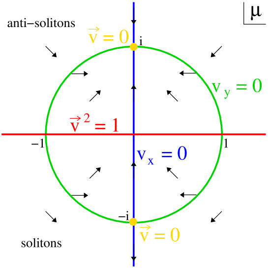
Figure 1: Soliton velocity $\vec{\mathrm{v}}$ as a function of $\mu$

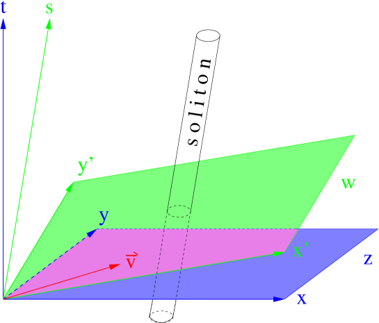
Figure 2: Soliton worldline in reference and rest frames

8 BPS conditions

Recall the vanishing-residue conditions (6.4),

$$\bigl{(}\boldsymbol{1}\ +\ \Sigma_{k}\bigr{)}\,S_{k}\ =\ 0\ =\ \bigl{(}\boldsymbol{1}\ +\ \Sigma_{k}\bigr{)}\,\bar{L}_{k}^{{\cal A},{\cal B},{\cal C}}\,S_{k}\ ,$$ (8.1)

where $\Sigma_{k}$ abbreviates the sum over $\ell$. The left equation, which arose from the reality condition (6.1), will be solved a bit later, using the multiplicative form of the ansatz (6.3). For the right equation, which represents the linear system (6.2) and therefore the equation of motion, the differential operators simplify in the co-moving coordinates to

$$\bar{L}_{k}^{{\cal A}}\ =\ \bar{L}_{k}^{\cal B}\ =\ (\mu_{k}{-}\bar{\mu}_{k})\frac{\partial}{\partial\bar{w}_{k}}\ =:\ \bar{L}_{k}\qquad{\text{and}}\qquad\bar{L}_{k}^{{\cal C}}\ =\ (\mu_{k}{-}\bar{\mu}_{k})\frac{\partial}{\partial\bar{\eta}_{k}^{i}}\ =:\ \bar{L}_{k}^{i}\ .$$ (8.2)

Essentially, this means that $S_{k}$ does not depend on $\bar{w}_{k}$ or $\bar{\eta}_{k}^{i}$. However, since $(\boldsymbol{1}+\Sigma_{k})$ is not invertible, in view of the left equation in (8.1) slightly weaker conditions hold, namely

$$\bar{L}_{k}\,S_{k}\ =\ S_{k}\,\tilde{Z}_{k}\qquad{\text{and}}\qquad\,\bar{L}_{k}^{i}\,S_{k}\ =\ S_{k}\,\tilde{Z}_{k}^{i}\ .$$ (8.3)

In the operator formulation of the Moyal deformation, these read

$$c_{k}\,\hat{S}_{k}\ =\ \hat{S}_{k}\,\hat{Z}_{k}\qquad{\text{and}}\qquad{\textstyle\frac{\partial}{\partial\bar{\eta}_{k}^{i}}}\,\hat{S}_{k}\ =\ \hat{S}_{k}\,\hat{Z}_{k}^{i}\ .$$ (8.4)

To unclutter the formulae I drop the hats and temporarily suppress the label $k$. The noncommutative BPS equations then takes the form

$$c\,S\ =\ S\,Z\qquad{\text{and}}\qquad{\textstyle\frac{\partial}{\partial\bar{\eta}^{i}}}\,S\ =\ S\,Z^{i}\ ,$$ (8.5)

where solutions $S_{k}$ are parametrized by $Z$ and $Z^{i}$.

The goal is to find operator-valued $n{\times}r$ matrices $S(c,c^{\dagger},\eta^{j},\bar{\eta}^{j})$ for any choice of $r{\times}r$ matrices $Z^{(i)}(c,c^{\dagger},\eta^{j},\bar{\eta}^{j})$. Recall that $n$ is determined by the group U($n$) but $r$ is arbitrary and in general depends on $k$. The general solution to (8.5) is rather involved, but things simplify when I restrict myself to holomorphic parameter matrices

$$Z\ =\ Z(c,\eta^{j})\qquad{\text{and}}\qquad Z^{i}\ =\ Z^{i}(c,\eta^{j})\ .$$ (8.6)

9 Nonabelian BPS solutions

For holomorphic choices of $Z$ and $Z^{i}$ I can write down the general solution to (8.5) as

$$S\ =\ R(c,\eta^{i})\ :\!\exp\bigl{\{}Z(c,\eta^{j})\,c^{\dagger}-c\,c^{\dagger}\bigr{\}}\!:\ \exp\bigl{\{}\textstyle{\sum_{i}}Z^{i}(c,\eta^{j})\,\bar{\eta}^{i}\bigr{\}}\ Q(c,\eta^{j})\ ,$$ (9.1)

where $R_{n\times r}$ and $Q_{r\times r}$ are arbitrary holomorphic matrix functions of $c$ and $\eta^{j}$ and where the colons signify normal ordering with respect to the $(c,c^{\dagger})$ algebra. It turns out that

$$S\quad\to\quad S\,\Gamma\qquad{\text{and}}\qquad Z^{(i)}\quad\to\quad\Gamma^{-1}Z^{(i)}\,\Gamma$$ (9.2)

does not change the final solution $\Phi$ or $\Upsilon$ and, hence, invertible right factors in the solution (9.1) may be omitted. Without loss of generality, I therefore put $Z^{i}=0$. A regular matrix $Q$ allows me to simplify the solution (9.1) to

$$S\ =\ R(c,\eta^{i})\ :\!\exp\bigl{\{}Z(c,\eta^{j})\,c^{\dagger}-c\,c^{\dagger}\bigr{\}}\!:$$ (9.3)

and further to

$$S\ =\ R(c,\eta^{i})$$ (9.4)

if the normal-ordered exponential is invertible.

The prime example for the latter, holomorphic, case is

$$Z=\boldsymbol{1}_{r}\otimes c\qquad\Leftrightarrow\qquad[c\,,\,S]\ =\ 0\ ,$$ (9.5)

which immediately sets $S=R$. For $r{<}n$ I can interpret $S$ as a map

$$S:\ \mathbb{C}^{r}\otimes{\cal H}\ \hookrightarrow\ \mathbb{C}^{n}\otimes{\cal H}\ ,$$ (9.6)

and (8.5) says that this embedding is stable under the action of $c$ and of $\frac{\partial}{\partial\bar{\eta}^{i}}$. The ensueing solitons I call “nonabelian” because they require $n\geq 2$ and in the commutative ($\Theta{\to}0$) limit smoothly reproduce the undeformed (supersymmetric) Ward-model solitons.

10 Abelian BPS solutions

The situation is different in the (more general) case where $:\!\e^{-c^{\dagger}(c-Z)}\!:$ has a nonzero kernel. In particular, this occurs whenever the $r{\times}r$ matrix $Z$ is not operator-valued, i.e.

$$Z=Z(\eta^{j})\qquad\Rightarrow\qquad:\!\e^{-c^{\dagger}(c-Z)}\!:\ =\ \e^{Zc^{\dagger}}:\!\e^{-c^{\dagger}c}\!:\ =\ \e^{Zc^{\dagger}}\,|\mathrm{v}\rangle\langle\mathrm{v}|\ =:\ |Z\rangle\langle\mathrm{v}|\ ,$$ (10.1)

where I defined an $r{\times}r$ matrix $|Z\rangle$ of (unnormalized) coherent states (eigenstates of $c$), whose parameters are still functions of the $\eta^{j}$. Recalling the freedom of right multiplication with $Q$, the resulting solution reads

$$S\ =\ R(c,\eta^{i})\,:\!\e^{-c^{\dagger}(c-Z(\eta^{j}))}\!:\,Q(c,\eta^{i})\ =\ R(Z,\eta^{j})\ |Z\rangle\langle*|$$ (10.2)

with an arbitrary $r{\times}r$ matrix $\langle*|$ of bras.

Clearly, the factor of $|Z\rangle\langle*|$ may not be dropped here. However, I can strip off the $\langle*|$ piece by generalizing $S$ to any $c$-stable embedding $Y\hookrightarrow\mathbb{C}^{n}\otimes{\cal H}$. For $\textrm{dim}Y\equiv q<\infty$ an embedding is just an $n{\times}q$ array of kets,

$$|S\rangle:\ \mathbb{C}^{q}\ \hookrightarrow\ \mathbb{C}^{n}\otimes{\cal H}\ ,$$ (10.3)

and the BPS conditions (8.5) become

$$c\,|S\rangle\ =\ |S\rangle\,Z(\eta^{j})\qquad{\text{and}}\qquad{\textstyle\frac{\partial}{\partial\bar{\eta}^{i}}}\,|S\rangle\ =\ |S\rangle\,Z^{i}(\eta^{j})\ .$$ (10.4)

Please note that $n=1$ is now possible, i.e. there exist novel solitons in the noncommutative U(1) model! Keeping $Z^{i}=0$ and removing $Q(\eta^{i})$, the BPS solution takes the form

$$|S\rangle\ =\ R(c,\eta^{i})\ \e^{Z(\eta^{j})c^{\dagger}}\,|\mathrm{v}\rangle\ =\ R(Z,\eta^{j})\ |Z\rangle\ .$$ (10.5)

Generically, I can employ the right multiplication with $Q$ to diagonalize

$$Z=\text{diag}\,(\alpha^{1},\ldots,\alpha^{q})\qquad\Rightarrow\qquad|Z\rangle\ =\ \text{diag}\,\bigl{(}|\alpha^{1}\rangle,\ldots,|\alpha^{q}\rangle\bigr{)}\qquad\text{with}\quad|\alpha^{l}\rangle:=\e^{\alpha^{l}(\eta^{j})c^{\dagger}}|\mathrm{v}\rangle\ .$$ (10.6)

From the Moyal-Weyl correspondence $|\mathrm{v}\rangle\langle\mathrm{v}|\ \leftrightarrow\ 2\,\e^{-w\bar{w}/\Theta}$ it is obvious that these solutions become singular in the commutative ($\Theta{\to}0$) limit. Therefore, I call them “abelian solutions”.

11 One-soliton configuration

I now build up the full soliton comfigurations from the building blocks $S_{k}$ or $|S_{k}\rangle$. Let me first present the simplest case, namely $m=1$, and suppress the index $k$. The ansatz (6.3) reduces to

$$\psi_{1}\ \ =\ \ \boldsymbol{1}\ +\ \frac{\mu-\bar{\mu}}{\zeta-\mu}\,P\ \ =\ \ \boldsymbol{1}\ +\ \frac{\Lambda\ S^{\dagger}}{\zeta-\mu}\ .$$ (11.1)

This is a good moment to work out the reality condition (6.1) in terms of the operator-valued $n{\times}n$ matrix $P$. The vanishing of the residue at $\zeta{=}\bar{\mu}$ immediately yields

$$P\ =\ P^{\dagger}\ =\ P^{2}\qquad\Rightarrow\qquad P\ =\ T\,\frac{1}{T^{\dagger}T}\,T^{\dagger}\quad\text{or}\quad\ =\ |T\rangle\,\frac{1}{\langle T|T\rangle}\,\langle T|\ .$$ (11.2)

Similarly, the linear system (6.2) is residue-free for

$$(\boldsymbol{1}{-}P)\,c\,P\ =\ 0\quad \Rightarrow \quad\quad c\,T\ =\ T\,Z\ \qquad\text{or}\qquad\quad c\,|T\rangle\ =\ |T\rangle\,Z\ ,$$ (11.3)

$$(\boldsymbol{1}{-}P)\,{\textstyle\frac{\partial}{\partial\bar{\eta}^{i}}}\,P\ =\ 0\quad \Rightarrow \quad\,{\textstyle\frac{\partial}{\partial\bar{\eta}^{i}}}\,T\ =\ T\,Z^{i}\qquad\text{or}\qquad{\textstyle\frac{\partial}{\partial\bar{\eta}^{i}}}\,|T\rangle\ =\ |T\rangle\,Z^{i}\ .$$ (11.4)

Comparison with (8.5) and (10.4) shows that $T=S$ and $\Lambda=(\mu{-}\bar{\mu})T\frac{1}{T^{\dagger}T}$ in this situation. Borrowing from the previous two sections, I generically have

$$T\ \ =\ \ \,S\ = R(c,\eta^{j})_{n\times r}\ ,\qquad\text{e.g. polynomials in $(c,\eta^{j})$}\ ,$$ (11.5)

$$|T\rangle\ =\ |S\rangle = R(c,\eta^{j})_{n\times q}\ \biggl{(}\begin{smallmatrix}|\alpha^{1}(\eta^{j})\rangle&&\\[-6.0pt] &\ddots&\\ &&|\alpha^{q}(\eta^{j})\rangle\end{smallmatrix}\biggr{)}_{q\times q}\ .$$ (11.6)

I remark that each matrix element of $R$ enjoys an $\eta$-expansion

$$R(c,\eta^{i})\ =\ R_{0}(c)+\eta^{i}R_{[i]}(c)+\eta^{i}\eta^{j}R_{[ij]}(c)+\eta^{i}\eta^{j}\eta^{k}R_{[ijk]}(c)+\eta^{i}\eta^{j}\eta^{k}\eta^{l}R_{[ijkl]}(c)\ ,$$ (11.7)

and $c$ acting on a coherent state $|\alpha^{l}\rangle$ may be replaced by its eigenvalue $\alpha^{l}$. From the above expressions it is only a matter of diligence to obtain the prepotentials via

$$\Phi\ =\ \boldsymbol{1}\ -\ (1{-}{\textstyle\frac{\mu}{\bar{\mu}}})P\qquad{\text{and}}\qquad\Upsilon\ =\ (\mu{-}\bar{\mu})P$$ (11.8)

and hence any other quantity one desires. Finally I remark that nonabelian and abelian solutions are distinguished by the rank of the projector $P$: in the former case $P$ has infinite rank in $\mathbb{C}^{n}\otimes{\cal H}$ but finite matrix rank $r$ in $\mathbb{C}^{n}$, while in the latter case $P$ is of finite rank $q$ in $\mathbb{C}^{n}\otimes{\cal H}$.

12 ${\cal N}$-extended multi-soliton configurations

The real benefit of integrability is the existence of multi-soliton solutions to our sigma-model equations (4.8)–(4.11) or quadratic equations (4.12)–(4.15). The dressing method provides me with an iterative scheme to build increasingly complex classical configurations, adding one lump at a time. First, the ansatz (6.3) contains $m$ pole positions $\mu_{k}$, which we take from the lower complex plane to exclude anti-solitons. Each $\mu_{k}$ gives rise to its own co-moving coordinate $w_{k}$ and, via Moyal deformation, to a Heisenberg pair $(c_{k},c_{k}^{\dagger})$ with its own vacuum $|\mathrm{v}_{k}\rangle$. Using the additive form of the ansatz, I have shown how to build nonabelian or abelian BPS solutions $S_{k}$ or $|S_{k}\rangle$ on this vacuum. Second, the multiplicative form of the ansatz generates conditions on the projectors $P_{k}$ and thus on the corresponding $T_{k}$ or $|T_{k}\rangle$. These conditions easily allow one to relate $T_{k}$ with $S_{k}$ in general,

$$T_{1}\ =\ S_{1}\qquad{\text{and}}\qquad T_{k}\ =\ \biggl{\{}\prod\limits_{\ell=1}^{k-1}\Bigl{(}\boldsymbol{1}\ -\ \frac{\mu_{k-\ell}-\bar{\mu}_{k-\ell}}{\mu_{k-\ell}-\bar{\mu}_{k}}\ P_{k-\ell}\Bigr{)}\biggr{\}}\ S_{k}\qquad\text{for}\quad k\geq 2\ ,$$ (12.1)

from which the projectors

$$P_{k}\ =\ T_{k}\,\frac{1}{T_{k}^{\dagger}T_{k}}\,T_{k}^{\dagger}\qquad\text{or}\quad P_{k}\ =\ |T_{k}\rangle\,\frac{1}{\langle T_{k}|T_{k}\rangle}\,\langle T_{k}|$$ (12.2)

are readily expressed in terms of the matrices $R_{k}$ and $Z_{k}^{(i)}$, whose size may vary with $k$. These matrices contain all moduli of the multi-soliton configuration besides the “rapidities” $\mu_{k}$. With the projectors in hand, I do not need the form of the $\Lambda_{mk}$, and the prepotentials are known as

$$\Phi\ =\prod_{\ell=0}^{m-1}\bigl{(}\boldsymbol{1}-(1{-}{\textstyle\frac{\mu_{m-\ell}}{\bar{\mu}_{m-\ell}}})P_{m-\ell}\bigr{)}\quad\ \text{and}\ \quad\Upsilon\ =\sum_{k=1}^{m}(\mu_{k}{-}\bar{\mu}_{k})P_{k}\ .$$ (12.3)

As the simplest example let me present the U(1) two-soliton ($n{=}1$, $m{=}2$) with ranks $q_{1}=q_{2}=1$. For $n{=}1$, the row matrix $R$ in (11.6) affects only the normalization of the coherent states $|\alpha^{l}\rangle$ and is thus irrelevant. It remains the two rapidities $\mu_{1}$ and $\mu_{2}$ as well as two complex coherent-state parameters $\alpha_{1}$ and $\alpha_{2}$, which may be functions of the Grassmann coordinates $\eta^{i}$. The result of the given recipe eventually produces the Yang-type prepotential

$$\Phi^{\dagger}\ =\ \boldsymbol{1}\ -\ \frac{1}{1-\mu|\sigma|^{2}}\,\Bigl{[}\,\frac{\mu_{11}}{\mu_{1}}|1\rangle\langle 1|\ +\ \frac{\mu_{22}}{\mu_{2}}|2\rangle\langle 2|\ -\ \sigma\mu\frac{\mu_{21}}{\mu_{2}}|1\rangle\langle 2|\ -\ \bar{\sigma}\mu\frac{\mu_{12}}{\mu_{1}}|2\rangle\langle 1|\,\Bigr{]}$$ (12.4)

with ($k=1,2$)

$$|k\rangle\ \propto\ |\alpha_{k}\rangle\ ,\qquad\langle k|k\rangle=1\ ,\qquad\langle 1|2\rangle\ =:\ \sigma\ ,\qquad\mu_{ij}\ :=\ \mu_{i}{-}\bar{\mu}_{j}\ ,\qquad\mu\ :=\ \frac{\mu_{11}\,\mu_{22}}{\mu_{12}\,\mu_{21}}\ ,$$ (12.5)

and the time dependence hides in the squeezing operators $U_{k}(t)$ that relate the vacua $|\mathrm{v}_{k}\rangle$ (on which the $|\alpha_{k}\rangle$ are built) to the reference vacuum $|0\rangle$ (see (7.4)).

13 Outlook

I have arrived at explicit multi-soliton configurations on $\mathbb{R}^{2,1|2{\cal N}}$, which formally look like the solutions in the non-supersymmetric model, except for additional dependencies on the chiral Grassmann coordinates $\eta^{i}$ via the matrices $R_{k}(c_{k},\eta_{k}^{j})$ and the parameters $\alpha_{k}^{l}(\eta_{k}^{j})$ entering $S_{k}$ and $|S_{k}\rangle$. Furthermore, the Grassmann-odd components in any $\eta$-expansion, such as (11.7), require the introduction of extraneous Grassmann-odd moduli $\varepsilon_{i}$, like in $R=R_{0}+\eta^{i}\varepsilon_{i}R^{\prime}+\ldots$.

As a simple example, consider the static abelian rank-one soliton ($\mu{=}-\mathrm{i}\leftrightarrow\mathrm{v}{=}0$), based on a coherent state

$$|T\rangle\ =\ \e^{\alpha(\eta^{i})a^{\dagger}}\,|0\rangle\ =\ \sum_{p=0}^{4}\alpha_{b}^{p}(a^{\dagger})^{p}|\alpha_{s}\rangle\ ,$$ (13.1)

with (subscripts referring to “body” and “soul”)

$$\alpha(\eta^{i})\ =\ \alpha_{b}+\alpha_{s}\ =\ \alpha_{b}+\eta^{i}\alpha_{[i]}+\eta^{i}\eta^{j}\alpha_{[ij]}+\eta^{i}\eta^{j}\eta^{k}\alpha_{[ijk]}+\eta^{i}\eta^{j}\eta^{k}\eta^{l}\alpha_{[ijkl]}\ .$$ (13.2)

Simplifying to $\alpha_{b}{=}0$ so that $\alpha^{5}=\alpha_{s}^{5}=0$, the projector becomes

$$P = \Bigl{(}{\textstyle\sum_{p=0}^{4}}\,p!(\bar{\alpha}_{s}\alpha_{s})^{p}\Bigr{)}^{-1}\ \sum_{k,l=0}^{4}{\textstyle\frac{\alpha_{s}^{k}\bar{\alpha}_{s}^{l}}{k!l!}}\,|k\rangle\langle l|$$ (13.3)

$$= (1-\bar{\alpha}_{s}\alpha_{s}+\ldots)\,\bigl{(}|0\rangle\langle 0|+\alpha_{s}|1\rangle\langle 0|+\bar{\alpha}_{s}|0\rangle\langle 1|+\alpha_{s}\bar{\alpha}_{s}|1\rangle\langle 1|+\ldots\bigr{)}\ .$$ (13.4)

For ${\cal N}{=}1$, I must put $\alpha_{s}=\eta\varepsilon$ with $\varepsilon^{2}=0$ and get

$$P\ =\ |0\rangle\langle 0|\ +\ \eta\varepsilon\,|1\rangle\langle 0|\ -\ \bar{\eta}\bar{\varepsilon}\,|0\rangle\langle 1|\ +\ \eta\bar{\eta}\varepsilon\bar{\varepsilon}\,\bigl{(}|1\rangle\langle 1|-|0\rangle\langle 0|\bigr{)}\ .$$ (13.5)

Employing the Moyal-Weyl map, this shows how the supersymmetric extension modifies the profile of the basic soliton. I have also checked the simplest U(2) examples, e.g. $T=\bigl{(}\begin{smallmatrix}\alpha(\eta)\\ a+\beta(\eta)\end{smallmatrix}\bigr{)}$, with similar results. In all cases, the topological charge is determined by the body component alone.

One would also like to investigate the energy density of such solitons. However, beyond the static ${\cal N}{=}1$ configurations, no action or energy functional is known for our ${\cal N}$-extended sigma models, so this remains a challenge.

How about scattering? To learn about the lump-lump interaction inside a non-static multi-soliton solution, I focus on the large-time asymptotics. It is easy to see that, in the $(t,x,y)$ frame, a moving lump yields

$$T\quad\buildrel{|t|\to\infty}\over{\longrightarrow}\quad t^{q}\ \Gamma\qquad\Rightarrow\qquad P\quad\buildrel{|t|\to\infty}\over{\longrightarrow}\quad\Pi\ =\ \Gamma\,{\textstyle\frac{1}{\Gamma^{\dagger}\Gamma}}\,\Gamma^{\dagger}$$ (13.6)

with a constant $n{\times}r$ matrix $\Gamma$, so that

$$\lim_{t\to\pm\infty}\Phi_{m}\ =\ \bigl{(}\boldsymbol{1}-(1{-}{\textstyle\frac{\mu_{m}}{\bar{\mu}_{m}}})\Pi_{m}\bigr{)}\cdots\bigl{(}\boldsymbol{1}-(1{-}{\textstyle\frac{\mu_{2}}{\bar{\mu}_{2}}})\Pi_{2}\bigr{)}\bigl{(}\boldsymbol{1}-(1{-}{\textstyle\frac{\mu_{1}}{\bar{\mu}_{1}}})\Pi_{1}\bigr{)}\ .$$ (13.7)

If the $k$th lump is static, $\Pi_{k}$ must be replaced by $P_{k}$. The important message here is that

$$\lim_{t\to+\infty}\Phi_{m}\ =\ \lim_{t\to-\infty}\Phi_{m}\ ,$$ (13.8)

which proves that the individual lumps in these multi-soliton configurations do not feel each other at all, but keep moving along their straight trajectories with constant velocities in the Moyal plane. When two lumps’ velocities coincide, however, the situation changes. In the limit of vanishing relative velocities a new time dependence is known to emerge for the non-supersymmetric Ward solitons, giving rise to breather-type and to nonabelian scattering configurations [5, 12]. I expect this feature to carry over to the models considered here.

Finally, one may ask why I have deformed only the bosonic coordinates but not also the fermionic ones. The reason was merely a practical one; the more general case of Moyal-deforming the whole $\mathbb{R}^{2,1|2{\cal N}}$ superspace is an obvious next step. Of special interest may be the other extreme, a purely fermionic deformation. It should lead to non-anticommuting solitons based on the Clifford algebra

$$\{\eta_{i}^{\alpha}\,,\,\eta_{j}^{\beta}\}\ =\ C_{ij}^{\alpha\beta}\ .$$ (13.9)

I foresee the corresponding BPS solutions to break part of the supersymmetry and perhaps carry additional structure interpretable as spin.

I thank C. Gutschwager, T.A. Ivanova and A.D. Popov for various fruitful discussions and collaborations. This work was partially supported by the Deutsche Forschungsgemeinschaft.

References

References

- [1] Ooguri H and Vafa C 1990 Mod. Phys. Lett. A 5 1389; Ooguri H and Vafa C 1991 Nucl. Phys. B 361 469
- [2] Ward R S 1988 J. Math. Phys. 29 386; Ward R S 1988 Commun. Math. Phys. 128 319
-
[3]
Lechtenfeld O, Popov A D and Spendig B 2001
J. High Energy Phys. JHEP06(2001)011
(Preprint hep-th/0103196) - [4] Lechtenfeld O and Popov A D 2001 J. High Energy Phys. JHEP11(2001)040 (Preprint hep-th/0106213)
- [5] Lechtenfeld O and Popov A D 2001 Phys. Lett. B 523 178 (Preprint hep-th/0108118)
- [6] Bieling S 2002 J. Phys. A 35 6281 (Preprint hep-th/0203269)
- [7] Wolf M 2002 J. High Energy Phys. JHEP06(2002)055 (Preprint hep-th/0204185)
- [8] Ihl M and Uhlmann S 2003 Int. J. Mod. Phys. A 18 4889 (Preprint hep-th/0211263)
-
[9]
Lechtenfeld O, Mazzanti L, Penati S, Popov A D and Tamassia L 2005
Nucl. Phys. B 705 477
(Preprint hep-th/0406065) -
[10]
Domrin A V, Lechtenfeld O and Petersen S 2005
J. High Energy Phys. JHEP03(2005)045
(Preprint hep-th/0412001) - [11] Chu C-S and Lechtenfeld O 2005 Phys. Lett. B 625 145 (Preprint hep-th/0507062)
-
[12]
Klawunn M, Lechtenfeld O and Petersen S 2006
J. High Energy Phys. JHEP06(2006)028
(Preprint hep-th/0604219) - [13] Popov A D 2007 Phys. Lett. B 647 509 (Preprint hep-th/0702106)
- [14] Lechtenfeld O and Popov A D 2007 J. High Energy Phys. JHEP06(2007)065 (Preprint arXiv:0704.0530)