Generation of large scale magnetic fields by coupling to curvature and dilaton field

Abstract

We investigate the generation of large scale magnetic fields in the universe from quantum fluctuations produced in the inflationary stage. By coupling these quantum fluctuations to the dilaton field and Ricci scalar, we show that the magnetic fields with the strength observed today can be produced. We consider two situations: First, the evolution of dilaton ends at the onset of the reheating stage. Second, the dilaton continues its evolution after reheating and then decays. In both cases, we come back to the usual Maxwell equations after inflation and then calculate present magnetic fields.

Department of Physics, Isfahan University of Technology, Isfahan 84156, Iran

PACS numbers: 98.80.Cq, 98.62.En

Key Words: Large Scale, Magnetic Fields, Inflation

1 Introduction

It is well understood that magnetic fields are present on various scales in the universe. These scales vary from planet size to clusters of galaxies of Mpc order[1]. The problem of obtaining a reasonable mechanism for generation of such a large scale magnetic field is an important question in modern cosmology because of its direct influence on the evolution of universe and astrophysical events. Magnetic fields have an important role in the dynamics of galaxies by confining the cosmic rays or transferring angular momentum away from protostellar clouds so that they may collapse to become stars (without the loss of angular momentum, protostellar clouds would collapse to a low-density centrifugally supported, unstarlike state). They also play an important role in the dynamics of pulsars, white dwarfs, and even black holes. The strength of these magnetic fields varies from $\mu$G in galaxies and cluster of galaxies to a few G in planets and up to $10^{12}$ G in neutron stars.

Some mechanisms known as galactic dynamo are established to amplify the scale and strength of magnetic fields by transforming the kinetic energy of turbulent motion of interstellar medium into magnetic energy. The gravitational collapse of matter to form galaxies and cluster of galaxies is definitely an amplification mechanism that can affect the strength of these fields because of the magnetic flux conservation. These mechanisms, however, are only amplification mechanisms and require a seed magnetic field to amplify to strengths presently observed . Theories established for generation of these seed fields are classified into two groups: astrophysical processes and cosmological processes in the early universe.

If the scale of magnetic fields of galaxies and cluster of galaxies are in the order of Kpc and Mpc, it means that we should investigate their origin in the early universe rather than in astrophysical processes. Then, these seed magnetic fields are trapped in highly conductive plasma collapsed to form structures like galaxies and their clusters during an adiabatic compression and, finally, subjected to some amplification mechanism like the galactic dynamo.

Many different mechanisms have been proposed for generation of these seed magnetic fields in the early universe [4] that may be classified as follows :

1. Breaking of conformal invariance of electromagnetic interaction at inflationary stage. This can be realized either through new non-minimal (and possibly non gauge invariant) coupling of electromagnetic field to curvature [5], or in dilaton electrodynamics [6], or by the well known conformal anomaly in the trace of the stress tensor induced by quantum corrections to Maxwell electrodynamics [7].

2. First order phase transitions in the early universe producing bubbles of new phase inside the old one [8]. A different mechanism but also related to phase transitions is connected with topological defects, in particular, cosmic strings [9].

3. Creation of stochastic inhomogeneities in cosmological charge asymmetry, either electric [10], or e.g. leptonic [11], at large scales which produce turbulent electric currents and, in turn, magnetic fields.

It seems that inflation is the most natural way for overcoming the large correlation scale [5, 12]. Inflation produces effects on scales much larger than Hubble horizon in a natural way. Then, if electromagnetic quantum fluctuations had been produced in that epoch, they could have been present as large scale magnetic fields today. The idea is based on the assumption that a quantum mechanical mode (in scales much smaller than Hubble Horizon) is excited which freezes when passing through the horizon. The problem arises from the fact that conformally invariant theory can not produce nonmassive particles in a conformally flat gravitational background. This is what happens to photons in a FRW background and, therefore, electromagnetic fields can not be produced. And if the origin of magnetic fields of galaxies and cluster of galaxies were quantum fluctuations produced in the inflationary stage, then conformal invariance of Maxwell theory should have been broken in that epoch. This happens in several ways [4].

We break the conformal invariance of Maxwell theory by coupling gravity (Ricci scalar)and a scalar field (dilaton) to it. A non-minimal coupling of electromagnetic fields to gravity was introduced first by Turner and Widrow [5]. Also, the coupling of a scalar field to electromagnetic fields has been studied by different people [5, 6, 13, 17]. We mix these two situations and consider the more realistic condition that both gravity and a scalar field, that is dilaton field, are coupled to electromagnetic field during the inflationary era. In [5], the problem is solved qualitatively and different values for magnetic fields are derived by changing the parameters. On the other hand, the problem is treated parametrically and more quantitatively in [13]. By integrating these solutions, we get a more generalized situation in which the coupling parameters are fixed by using some special values for the magnetic field.

We first introduce our theory, then derive equations of motion and solve them to get an expression for electromagnetic vector potential, $A_{\mu}$. Then we derive the evolution of electric and magnetic fields before and after inflation by using joining conditions. We assume two situations here :

1. Evolution of dilaton field ends by finishing inflation when dilaton freezes.

2. A more realistic situation in which dilaton continues its evolution after reheating and then decays into radiation.

Finally, we calculate today’s strength of magnetic fields on different scales.

2 Action and the equations of motion

For investigating the evolution of magnetic fields produced by a Maxwell theory whose conformal invariance is broken, we first introduce the lagrangian. We will then derive the equations of motion [5, 6, 13].

We introduce inflaton and dilaton scalar fields lagrangian density as

$${\cal L}_{dil}=-\frac{1}{2}g^{\mu\nu}{\partial}_{\mu}{\Phi}{\partial}_{\nu}{\Phi}-V[\Phi]\;,$$ (1)

$${\cal L}_{inf}=-\frac{1}{2}g^{\mu\nu}{\partial}_{\mu}{\phi}{\partial}_{\nu}{\phi}-U[\phi]\;,$$ (2)

$$V[\Phi]=\bar{V}\exp(-\bar{\lambda}\kappa\Phi)\;.$$ (3)

$U[\phi]$ and $V[\Phi]$ are inflaton and dilaton potentials, $\bar{\lambda}$ is constant and $\kappa=\frac{8\pi}{M_{PL}^{2}}$. The forms of $U[\phi]$ and $V[\Phi]$ are determined from higher dimension theories reduced to four dimensions [15, 16, 17].

The lagrangian density of electromagnetic field coupled to the dilaton and gravity is

$${\cal L}_{EM}=f(\Phi)(-\frac{1}{4}F_{\mu\nu}F^{\mu\nu}+\xi RA^{2})\;,$$ (4)

$$F^{\mu\nu}={\partial}^{\mu}A^{\nu}-{\partial}^{\nu}A^{\mu}\;,$$ (5)

$$R=6\left(\frac{\ddot{a}a+{\dot{a}}^{2}+k}{a^{2}}\right)\;.$$ (6)

$f(\Phi)$ and $\xi RA^{2}$ are dilaton and gravitational couplings to electromagnetic field, $k$ is curvature constant and $R$ is Ricci scalar [6]. $a$ is scale factor and $\xi$ is a dimensionless parameter which will be determined.

Therefore, the action is

$${\cal S}=\int d^{4}x\sqrt{-g}\hskip 8.53581pt[{\cal L}_{inf}+{\cal L}_{dil}+{\cal L}_{EM}]\;.\\$$ (7)

where $g$ is the metric tensor. We consider the metric of space-time as flat FRW metric (k=0)

$${ds}^{2}=g_{\mu\nu}dx^{\mu}dx^{\nu}={dt}^{2}-a^{2}(t)~{}d{\vec{x}}^{2}\;.\\$$ (8)

Our work is based on four assumptions:

1. In the inflationary stage with slow roll condition, the energy density of inflaton field is much bigger than that of the dilaton field, $\rho_{\phi}\gg\rho_{\Phi}$.

2. The universe becomes immediately hot after the inflationary stage, $t>t_{R}$.

3. The conductivity of the universe is ignorable in the inflationary stage because density of charged particles is very small in that epoch. After reheating, a lot of charged particles are produced so that conductivity immediately jumps to a large value after inflation, $\sigma_{c}\gg H$.

4. We consider two different situations for dilaton. First, the evolution of dilaton field ends by finishing inflation and the dilaton freezes; therefore, the coupling will be removed ($f=1$) [6]. Second, the dilaton continues its evolution after reheating until it reaches its minimum potential and then decays into radiation when again $f=1$ [13].

2.1 Equations of motion

From action (7), the inflaton, dilaton, and electromagnetic potential equations of motion are given by

$$-\frac{1}{\sqrt{-g}}{\partial}_{\mu}(\sqrt{-g}g^{\mu\nu}{\partial}_{\nu}\phi)+\frac{dU[\phi]}{d\phi}=0\;,$$ (9)

$$-\frac{1}{\sqrt{-g}}{\partial}_{\mu}(\sqrt{-g}g^{\mu\nu}{\partial}_{\nu}\Phi)+\frac{dV[\Phi]}{d\Phi}=\frac{df(\Phi)}{d\Phi}\left(-\frac{1}{4}F_{\mu\nu}F^{\mu\nu}+\xi RA^{2}\right)\;,$$ (10)

$$-\frac{1}{\sqrt{-g}}{\partial}_{\mu}(\sqrt{-g}f(\Phi)F^{\mu\nu}-2\xi RA^{\nu})=0\;.$$ (11)

Since every inhomogeneity of space will be diluted in the inflationary stage, we can ignore the spatial dependence of the inflaton and the dilaton scalar fields. The right hand side of Eq.(10) is very small and can be considered as a perturbation in the dilaton theory.

The inflaton and dilaton equations of motion are derived from Eqs.(9) and (10)

$$\ddot{\phi}+3H\dot{\phi}+\frac{dU[\phi]}{d\phi}=0\;,$$ (12)

$$\ddot{\Phi}+3H\dot{\Phi}+\frac{dV[\Phi]}{d\Phi}=0\;.$$ (13)

H is the Hubble constant and is derived from Friedman equation

$$H^{2}=\left(\frac{\dot{a}}{a}\right)^{2}=\frac{{\kappa}^{2}}{3}({\rho}_{\phi}+{\rho}_{\Phi})\;.\\$$ (14)

where

$${\rho}_{\phi}=\frac{1}{2}{\dot{\phi}}^{2}+U[\phi]\;,$$ (15)

$${\rho}_{\Phi}=\frac{1}{2}{\dot{\Phi}}^{2}+V[\Phi]\;.$$ (16)

are the inflaton and dilaton energy densities. Dot implies time derivatives and $\rho=\rho_{\phi}+\rho_{\Phi}$ is total density. According to our assumptions, $\rho_{\phi}\gg\rho_{\Phi}$ and we can ignore the dilaton energy density in the inflationary stage whereby we will have:

$$H^{2}\approx\frac{{\kappa}^{2}}{3}U[\phi]\equiv{H_{inf}}^{2}\;.\\$$ (17)

We have used slow roll condition in the above equation and $H_{inf}$ is the value of Hubble constant in the inflationary stage. Since we assume that the term $\xi RA^{2}$ is small compared to $F_{\mu\nu}F^{\mu\nu}$, we can use the Coulomb gauge, $A_{0}(t,\vec{x})=0$ and $\partial_{j}A^{j}(t,\vec{x})=0$, as used in the standard Maxwell theory. We derive equation of motion for electromagnetic potential $A$ (in comoving coordinate) from Eq.(11)

$$\ddot{A_{i}}(t,\vec{x})+\left(H+\frac{\dot{f}}{f}\right)\dot{A_{i}}(t,\vec{x})-\left(\frac{1}{a^{2}}{\partial}_{j}{\partial}_{j}-2\xi R\right)A_{i}(t,\vec{x})=0\;.\\$$ (18)

2.2 Electromagnetic potential $A$

To solve the equation of motion for $A$, we first quantize the theory. The corresponding momentum from ${\cal{L}}_{EM}$ is

$$\pi_{\nu}=\frac{\partial{\cal L}_{EM}}{\partial{\dot{A_{\nu}}}}\;,$$

$${\pi}_{0}=0,\hskip 14.22636pt{\pi}_{i}=f(\Phi)a(t)\dot{A_{i}}(t,\vec{x})\;.$$ (19)

Commutation relation for $A_{i}$ and $\pi_{i}$ is

$$[\hskip 1.42262ptA_{i}(t,\vec{x}),{\pi}_{j}(t,\vec{y})\hskip 1.42262pt]=i\int\frac{d^{3}k}{{(2\pi)}^{3}}e^{i\vec{k}\cdot(\vec{x}-\vec{y})}~{}~{}\left({\delta}_{ij}-\frac{k_{i}k_{j}}{k^{2}}\right)\;.\\$$ (20)

where $k$ is comoving wave number. Using these relations, we can write the quantum form of $A$ as [17]

$$A_{i}(t,\vec{x})=\int\frac{d^{3}k}{{(2\pi)}^{3/2}}[\hskip 1.42262pt\hat{b}(\vec{k})A_{i}(t,\vec{k})e^{i\vec{k}\cdot\vec{x}}+{\hat{b}}^{\dagger}(\vec{k}){A_{i}}^{*}(t,\vec{k})e^{-i\vec{k}\cdot\vec{x}}\hskip 1.42262pt]\;.\\$$ (21)

in which $\hat{b}$ and $\hat{b^{{\dagger}}}$ are annihilation and creation operators with the following commutation relations

$$[\hskip 1.42262pt\hat{b}(\vec{k}),{\hat{b}}^{\dagger}({\vec{k}}^{\prime})]\hskip 1.42262pt={\delta}^{3}(\vec{k}-{\vec{k}}^{\prime})\;,$$

$$[\hskip 1.42262pt\hat{b}(\vec{k}),\hat{b}({\vec{k}}^{\prime})\hskip 1.42262pt]=[\hskip 1.42262pt{\hat{b}}^{\dagger}(\vec{k}),{\hat{b}}^{\dagger}({\vec{k}}^{\prime})]\hskip 1.42262pt=0\;.$$ (22)

For simplicity, we choose $x_{1}$ along the direction of $\vec{k}$. Thus, from now on we will work only with two transverse components (I=2,3). Equation of motion for electromagnetic potential Fourier modes will be:

$$\ddot{A_{I}}(t,k)+\left(H_{inf}+\frac{\dot{f}}{f}\right)\dot{A_{I}}(t,k)+\left(\frac{k^{2}}{a^{2}}-2\xi R\right)A_{I}(t,k)=0\;.\\$$ (23)

Ricci scalar in the inflationary stage is $R=12H^{2}$ [12].

We get normalization condition for $A_{i}(t,k)$ from Eq.(20) as

$$A_{i}(t,k){\dot{A}}_{j}^{*}(t,k)-{\dot{A}}_{j}(t,k){A_{i}}^{*}(t,k)=\frac{i}{fa}\left({\delta}_{ij}-\frac{k_{i}k_{j}}{k^{2}}\right)\;.\\$$ (24)

For more simplicity in solving the equations, we use the following approximation for the evolution of $f(\Phi)$

$$f(\Phi)=f[\Phi(t)]=f[\hskip 1.42262pt\Phi(a(t))\hskip 1.42262pt]\equiv f_{0}a^{2\alpha-2}\;.\\$$ (25)

where $f_{0}$ is a constant and all time variations of $f(\Phi)$ have been put in $a^{2\alpha-2}$. It can be shown that time dependence of $\alpha$ can be ignored if we have slow roll condition for inflaton and dilaton fields [13]. The only problem that remains is determination of an acceptable range for variation of $\alpha$ that can be achieved from consistency conditions (section 4).

From Eq.(25)

$$H_{inf}+\frac{\dot{f}}{f}=(2\alpha-1)H_{inf}\;.\\$$ (26)

By introducing a new variable $d\eta=\frac{dt}{a}$, and relying on the fact that $\eta=-\frac{1}{aH_{inf}}$ in the inflationary stage ( in De’sitter spacetime ), we can rewrite eq.(23) as

$$\frac{d^{2}{A_{I}}(k,\eta)}{d{\eta}^{2}}+\left(\frac{1-2\alpha}{\eta}\right)\frac{d{A_{I}}(k,\eta)}{d\eta}+\left(k^{2}+\frac{24\xi}{{\eta}^{2}}\right){A_{I}}(k,\eta)=0\;.\\$$ (27)

One of the forms of Bessel Equation is

$$\frac{d^{2}{u}}{dz^{2}}+\left(\frac{1-2\nu}{z}\right)\frac{d{u}}{dz}+\left(\delta^{2}+\frac{{\nu}^{2}-{\nu^{\prime}}^{2}}{z^{2}}\right)u=0\;.\\$$ (28)

where $\nu$, $\nu^{\prime}$ and $\delta$ are positive and the solution is

$$u=z^{\nu}(D_{1}H_{\nu^{\prime}}^{(1)}(\delta z)+D_{2}H_{\nu^{\prime}}^{(2)}(\delta z))\;.\\$$ (29)

$H_{\nu^{\prime}}^{(1)}$ and $H_{\nu^{\prime}}^{(1)}$ are Hankel functions of first and second order $\nu^{\prime}$, respectively. Comparing Eqs. (27) and (28), we will have

$$\eta=z~{}~{}~{}~{}~{}~{}~{}~{}~{}~{}~{}~{}~{}~{}~{}~{}~{}~{}~{}\nu=\alpha~{}~{}~{}~{}~{}~{}~{}~{}~{}~{}~{}~{}~{}~{}~{}~{}~{}~{}~{}\delta=\pm k\;,$$ (30)

$$\nu^{\prime}=~{}\pm\sqrt{{\nu}^{2}-24\xi}~{}=~{}\pm\sqrt{{\alpha}^{2}-24\xi}\;.$$ (31)

The solution obtained for Eq.(27) is

$$A_{I}(k,\eta)=D_{1}(a){(-H_{inf}\eta)}^{\nu}H_{{\nu}^{\prime}}^{(1)}(-k\eta)+D_{2}(a)(-H_{inf}\eta)^{\nu}H_{\nu^{\prime}}^{(2)}(-k\eta)\;.\\$$ (32)

$D_{1}$ and $D_{2}$ coefficients are determined from the renormalization relation (24)

$$|D_{1}(a)|^{2}-|D_{2}(a)|^{2}=\frac{\pi}{4H_{inf}f(a)}~{}a^{2\nu-1}\;.\\$$ (33)

For simplicity, we choose

$$D_{1}(a)=\sqrt{\frac{\pi}{4H_{inf}}f(a)}~{}~{}a^{\nu-1/2}\hskip 2.84526pte^{i(\nu^{\prime}+1)\pi/4}\hskip 14.22636ptD_{2}(a)=0\;.\\$$ (34)

Since we are working with large scale magnetic fields, we expand Eq.(32) whithin large wavelength limit for $\nu>0$ and $\nu<0$

$$A_{I}(k,a)=2^{\nu^{\prime}}\sqrt{\frac{1}{4\pi H_{inf}f(a)}}\Gamma(\nu^{\prime})a^{-1/2}$$

$$~{}~{}~{}~{}~{}~{}~{}~{}{\left(\frac{k}{aH_{inf}}\right)}^{-\nu^{\prime}}e^{i(\nu^{\prime}-1)\pi/4}~{}~{}~{}~{}~{}~{}\nu^{\prime}>0\;,$$ (35)

$$A_{I}(k,a)=2^{-\nu^{\prime}}\sqrt{\frac{1}{4\pi H_{inf}f(a)}}\Gamma(-\nu^{\prime})a^{-1/2}$$

$$~{}~{}~{}~{}~{}~{}~{}~{}{\left(\frac{k}{aH_{inf}}\right)}^{\nu^{\prime}}e^{i(3-\nu^{\prime})\pi/4}~{}~{}~{}~{}~{}~{}\nu^{\prime}<0\;.$$ (36)

The electric and magnetic fields can be easily derived from the above expressions using the relation between $\vec{A}$ and $\vec{E}$ and $\vec{B}$ in comoving coordinate system.

3 Electric and magnetic fields evolution

In Coloumb gauge, electric and magnetic fields are derived from vector potential $A$ as follows

$$\vec{E}=-\frac{\partial}{\partial t}\vec{A},~{}~{}~{}~{}~{}~{}~{}~{}~{}~{}~{}~{}~{}\vec{B}=\vec{\nabla}\times\vec{A}\;.\\$$ (37)

In comoving coordinate, electric and magnetic fields are [17]

$${E_{i}}^{C}(t,\vec{x})=\dot{A_{i}}(t,\vec{x})\;,$$ (38)

$${B_{i}}^{C}(t,\vec{x})=\frac{1}{a}{\epsilon}_{ijk}\partial_{j}A_{k}(t,\vec{x})\;.$$ (39)

where ”c” implies comoving and $\partial_{j}$ is differentiation in comoving coordinate.

Using relations (35), (38), and (39), we can derive Fourier components of electric and magnetic fields in the inflationary stage

$${E_{I}}^{C}(k,a)=\sqrt{\frac{\pi}{4H_{inf}f(a)}}\hskip 3.41432pt(\frac{k}{a})a^{-1/2}[(\nu-1/2)H_{\nu^{\prime}}^{(1)}\left(\frac{k}{aH_{inf}}\right)$$

$$~{}~{}~{}~{}~{}~{}~{}~{}~{}~{}~{}~{}~{}+1/2\left(H_{\nu^{\prime}-1}^{(1)}\left(\frac{k}{aH_{inf}}\right)-H_{\nu^{\prime}+1}^{(1)}\left(\frac{k}{aH_{inf}}\right)e^{i(\nu^{\prime}+1)\pi/4}\right)]\,$$

$${B_{I}}^{C}(k,a)=-i(-1)^{I}\sqrt{\frac{\pi}{4H_{inf}f(a)}}$$

$$~{}~{}~{}~{}~{}~{}~{}~{}~{}~{}~{}~{}~{}\times\left(\frac{k}{a}\right)a^{-1/2}H_{\nu^{\prime}}^{(1)}\left(\frac{k}{aH_{inf}}\right)e^{i(\nu^{\prime}+1)\pi/4}\;.$$ (41)

We assumed that the dilaton freezes after inflation. In this epoch, the conductivity of the universe increases immediately so that $\sigma\gg H$ [6]. And the evolution of electromagnetic vector potential follows from the equation

$$\ddot{A_{i}}(t,\vec{x})+\left(\frac{\dot{a}}{a}+{\sigma}_{c}\right)\dot{A_{i}}(t,\vec{x})-\frac{1}{a^{2}}{\partial}_{j}{\partial}_{j}{A_{i}}(t,\vec{x})=0\;.\\$$ (42)

Ratra has shown that we have the following joining conditions for electric and magnetic fields at transition from the inflationary stage to the radiation dominated epoch ( $t=t_{R}$ ) [6, 18],

$${E^{C}}_{i(RD)}(t_{R},\vec{x})=\exp(-{\sigma}_{c}t_{R}){E^{C}}_{i(INF)}(t_{R},\vec{x})\;,$$ (43)

$$B^{C}_{i(RD)}(t_{R},\vec{x})=B^{C}_{i(INF)}(t_{R},\vec{x})\;.$$ (44)

According to these relations, in a universe with large conductivity, the electric field accelerates charged particles but it reduces exponentially. From Alf’ven theorem, the magnetic flux is conserved in a conductive universe and, therefore, the magnetic field evolution is by $a^{-2}$ in the physical coordinate system [6, 17, 18].

In the physical coordinate, the electric and magnetic fields are [17]

$${E_{i}}^{Ph}(t,\vec{x})=a^{-1}E_{i}^{C}(t,\vec{x})\;,$$ (45)

$${B_{i}}^{Ph}(t,\vec{x})=a^{-1}B_{i}^{C}(t,\vec{x})\;.$$ (46)

Using relations (39), (41) and (46) we have

$$|{B_{I}}^{Ph}(t,k)|^{2}\equiv a^{-2}|{B_{I}}^{C}(k,a)|^{2}$$

$$~{}~{}~{}~{}~{}~{}~{}~{}=a^{-2}\left(\frac{\pi}{4H_{inf}f(a)}\right){\left(\frac{k}{a}\right)}^{2}\left(\frac{1}{a}\right)H_{\nu^{\prime}}^{(1)}\left(\frac{k}{aH_{inf}}\right)H_{\nu^{\prime}}^{(2)}\left(\frac{k}{aH_{inf}}\right)\;.$$ (47)

We are considering the magnetic fields on large scales. Thus, we expand relation (47) for small k to note that the magnetic field evolves with $a^{-2}$ after inflation

$$|B_{I}^{Ph}(t,k)|^{2}=\frac{2^{2\nu^{\prime}-2}}{\pi}\Gamma^{2}(\nu^{\prime})f^{-1}(a_{R})$$

$$\hskip 99.58464pt\times\left(\frac{k^{2}}{a_{R}H_{inf}}\right){\left(\frac{k}{a_{R}H_{inf}}\right)}^{-2\nu^{\prime}}{\left(\frac{1}{a}\right)}^{4},\hskip 28.45274pt\hskip 3.98337pt\nu^{\prime}>0\;,$$ (48)

$$|B_{I}^{Ph}(t,k)|^{2}=\frac{2^{-2(\nu^{\prime}+1)}}{\pi}{\Gamma}^{2}(-\nu^{\prime})f^{-1}(a_{R})$$

$$\hskip 99.58464pt\times\left(\frac{k^{2}}{a_{R}H_{inf}}\right){\left(\frac{k}{a_{R}H_{inf}}\right)}^{2\nu^{\prime}}{\left(\frac{1}{a}\right)}^{4},\hskip 28.45274pt\hskip 3.98337pt\nu^{\prime}<0\;.$$ (49)

The magnetic energy density in the Fourier space is

$${\rho}_{B}(t,k)=\frac{1}{2}|{B_{t}}^{Ph}(t,k)|^{2}~{}f(a)\;.\\$$ (50)

Since two transverse components are equal, $B_{t}=\sqrt{2}B_{I}$. Multiplying (50) by phase space density $\frac{4\pi k^{3}}{3(2\pi)^{3}}$, the large scale magnetic field energy density in the coordinate space is

$${\rho}_{B}(L,t)=\frac{k^{3}}{6\pi^{2}}|{B_{I}}^{Ph}(t,k)|^{2}f(a)\;.\\$$ (51)

where $L=\frac{2\pi}{k}$ is correlation length.

By integrating Eqs.(48), (49) and (51), we obtain the magnetic field energy density on the scale $L=\frac{2\pi}{k}$

$${\rho}_{B}(L,t_{0})=\frac{2^{2|\nu^{\prime}|-3}}{3\pi^{3}}{\Gamma}^{2}(|\nu^{\prime}|){H_{inf}}^{4}\left(\frac{a_{R}}{a_{0}}\right)^{4}{\left(\frac{k}{a_{R}H_{inf}}\right)}^{-2|\nu^{\prime}|+5}\;.\\$$ (52)

Accoring to the above relation, the spectrum of the magnetic fields is invariant for $2|\nu^{\prime}|=5$.

4 Consistency condition

The energy density of electric and magnetic fields should be smaller than the energy density of dilaton field in the inflationary stage so that only $V[\Phi]$ determines the evolution of dilaton [17]. We show the ratio of electromagnetic energy density to dilaton energy density by $\Theta(L,t)$:

$$\Theta(L,t)\equiv\frac{1}{{\rho}_{\Phi}}[\hskip 1.42262pt{\rho}_{B}(L,t)+{\rho}_{E}(L,t)\hskip 1.42262pt]\;,$$ (53)

$${\rho}_{E}(L,t)=\frac{k^{3}}{6{\pi}^{2}}|{E_{I}}^{Ph}(t,k)|^{2}\hskip 0.85358ptf(a)\;.$$ (54)

If $\Theta\ll 1$, the consistency condition is satisfied. Using Eqs.(17), (3), (41), (53) and (54), we have

$$\Theta\approx\frac{1}{9w}\left(\frac{H_{inf}}{M_{Pl}}\right)^{2}[\left(\frac{k}{aH_{inf}}\right)^{5}\times[H_{\nu^{\prime}}^{(1)}\left(\frac{k}{aH_{inf}}\right)H_{\nu^{\prime}}^{(2)}\left(\frac{k}{aH_{inf}}\right)$$

$$+\left(\left(1/2\left(H_{\nu^{\prime}-1}^{(1)}\left(\frac{k}{aH_{inf}}\right)-H_{\nu^{\prime}+1}^{(1)}\left(\frac{k}{aH_{inf}}\right)\right)+\left(\nu-\frac{1}{2}\right)H_{\nu^{\prime}}^{(1)}\left(\frac{k}{aH_{inf}}\right)\right)\right)$$

$$\times\left(1/2\left(H_{\nu^{\prime}-1}^{(2)}\left(\frac{k}{aH_{inf}}\right)-H_{\nu^{\prime}+1}^{(2)}\left(\frac{k}{aH_{inf}}\right)\right)+\left(\nu-\frac{1}{2}\right)H_{\nu^{\prime}}^{(2)}\left(\frac{k}{aH_{inf}}\right)\right)]]$$

$$\;.$$ (55)

As a measure of $\Theta$, one may use the upper limit of $H_{inf}$ calculated from CMB anisotropy observations [19, 20, 21]

$$\frac{H_{inf}}{M_{Pl}}\leq 2\times 10^{-5}~{}~{}~{}~{}~{}~{}~{}\Longrightarrow~{}~{}~{}~{}~{}~{}~{}~{}H_{inf}=2.4\times 10^{14}GeV\;.\\$$ (56)

and noting that $\frac{k}{aH_{inf}}$ decreases with evolution of universe, from Eq.(55), we may conclude that when $\frac{k}{aH_{inf}}=1$, $\Theta<10^{-10}\omega^{-1}$ ( $\omega$ is defined as $\omega\equiv\frac{V[\Phi]}{\rho_{\phi}}\approx\frac{V[\Phi]}{U[\phi]}$ and according to our assumption that the dilaton energy density is much smaller than that of inflaton in the inflationary era, $\omega\ll 1$ ), the consistency condition exists. By investigating these relations within large wavelength limits, we have

$$\Theta\approx\frac{1}{9\pi^{2}w}{\left(\frac{H_{inf}}{M_{Pl}}\right)}^{2}[x^{-5+2\nu^{\prime}}2^{2\nu^{\prime}}\Gamma^{2}(\nu^{\prime})+1/4(2^{2(\nu^{\prime}-1)}\Gamma^{2}(\nu^{\prime}-1)x^{-2}$$

$$-2^{2\nu^{\prime}+1}\Gamma(\nu^{\prime}-1)\Gamma(\nu^{\prime}+1)+2^{(2\nu^{\prime}+1)}\Gamma^{2}(\nu^{\prime}+1)x^{2})+$$

$$(\nu-1/2)^{2}2^{2\nu^{\prime}}\Gamma^{2}(\nu^{\prime})+(\nu-1/2)(-2^{2(\nu^{\prime}+1)}\Gamma(\nu^{\prime}+1)\Gamma(\nu^{\prime})x$$

$$+2^{2\nu^{\prime}}\Gamma(\nu^{\prime})\Gamma(\nu^{\prime}-1)x^{-1})]]~{}~{}~{}~{}~{}~{}~{}~{}~{}~{}~{}~{}~{}~{}~{}~{}~{}~{}~{}~{}~{}~{}~{}~{}~{}~{}~{}~{}~{}~{}~{}~{}~{}~{}~{}~{}~{}~{}~{}~{}~{}~{}~{}~{}~{}~{}\nu^{\prime}>1\;,$$ (57)

$$\Theta\approx\frac{1}{9\pi^{2}w}{\left(\frac{H_{inf}}{M_{Pl}}\right)}^{2}[x^{-5+2\nu^{\prime}}2^{2\nu^{\prime}}\Gamma^{2}(\nu^{\prime})+1/4(2^{2(1-\nu^{\prime})}\Gamma^{2}(1-\nu^{\prime})x^{2(1-2\nu^{\prime})}$$

$$-2^{2}\Gamma(\nu^{\prime}+1)\Gamma(1-\nu^{\prime})x^{2(1-\nu^{\prime}}+2^{(2\nu^{\prime}+1)}\Gamma^{2}(\nu^{\prime}+1)x^{2})+(\nu-1/2)^{2}2^{2\nu^{\prime}}\Gamma^{2}(\nu^{\prime})$$

$$+(\nu-1/2)(2^{2}\Gamma(\nu^{\prime})\Gamma(1-\nu^{\prime})x^{1-2\nu^{\prime}}-2^{2\nu^{\prime}+1}\Gamma(\nu^{\prime})\Gamma(\nu^{\prime}+1)x)]$$

$$~{}~{}~{}~{}~{}~{}~{}~{}~{}~{}~{}~{}~{}~{}~{}~{}~{}~{}~{}~{}~{}~{}~{}~{}~{}~{}~{}~{}~{}~{}~{}~{}~{}~{}~{}~{}~{}~{}~{}~{}~{}~{}~{}~{}~{}~{}~{}~{}~{}~{}~{}~{}~{}~{}~{}~{}~{}~{}~{}~{}~{}~{}~{}~{}~{}~{}~{}~{}~{}~{}~{}~{}~{}~{}~{}~{}0<\nu^{\prime}<1\;,$$ (58)

$$\Theta\approx\frac{1}{9\pi^{2}w}{\left(\frac{H_{inf}}{M_{Pl}}\right)}^{2}[x^{-(5+2\nu^{\prime})}2^{-2\nu^{\prime}}\Gamma^{2}(-\nu^{\prime})+1/4(2^{2(1-\nu^{\prime})}\Gamma^{2}(1-\nu^{\prime})x^{2}$$

$$-2^{2}\Gamma(\nu^{\prime}+1)\Gamma(1-\nu^{\prime})x^{2}+2^{(2\nu^{\prime}+1)}\Gamma^{2}(\nu^{\prime}+1)x^{2(1+\nu^{\prime})})+(\nu-1/2)^{2}2^{-2\nu^{\prime}}\Gamma^{2}(-\nu^{\prime})$$

$$+(\nu-1/2)(-2^{2}\Gamma(-\nu^{\prime})\Gamma(1+\nu^{\prime})x^{1+2\nu^{\prime}}+2^{2(1-\nu^{\prime})}\Gamma(-\nu^{\prime})\Gamma(1-\nu^{\prime})x)]$$

$$~{}~{}~{}~{}~{}~{}~{}~{}~{}~{}~{}~{}~{}~{}~{}~{}~{}~{}~{}~{}~{}~{}~{}~{}~{}~{}~{}~{}~{}~{}~{}~{}~{}~{}~{}~{}~{}~{}~{}~{}~{}~{}~{}~{}~{}~{}~{}~{}~{}~{}~{}~{}~{}~{}~{}~{}~{}~{}~{}~{}~{}~{}~{}~{}~{}~{}~{}~{}~{}~{}~{}~{}~{}~{}~{}-1<\nu^{\prime}<0\;,$$ (59)

$$\Theta\approx\frac{1}{9\pi^{2}w}{\left(\frac{H_{inf}}{M_{Pl}}\right)}^{2}[x^{-(5+2\nu^{\prime})}2^{-2\nu^{\prime}}\Gamma^{2}(-\nu^{\prime})+1/4(2^{2(-\nu^{\prime}-1)}\Gamma^{2}(-\nu^{\prime}-1)x^{-2}$$

$$-2^{-2\nu^{\prime}+1}\Gamma(-\nu^{\prime}-1)\Gamma(-\nu^{\prime}+1)+2^{(-2\nu^{\prime}+1)}\Gamma^{2}(-\nu^{\prime}+1)x^{2})+(\nu-1/2)^{2}2^{-2\nu^{\prime}}\Gamma^{2}(-\nu^{\prime})$$

$$+(\nu-1/2)(-2^{2(-\nu^{\prime}+1)}\Gamma(-\nu^{\prime}+1)\Gamma(-\nu^{\prime})x+2^{-2\nu^{\prime}}\Gamma(-\nu^{\prime})\Gamma(-\nu^{\prime}-1)x^{-1})]$$

$$~{}~{}~{}~{}~{}~{}~{}~{}~{}~{}~{}~{}~{}~{}~{}~{}~{}~{}~{}~{}~{}~{}~{}~{}~{}~{}~{}~{}~{}~{}~{}~{}~{}~{}~{}~{}~{}~{}~{}~{}~{}~{}~{}~{}~{}~{}~{}~{}~{}~{}~{}~{}~{}~{}~{}~{}~{}~{}~{}~{}~{}~{}~{}~{}~{}~{}~{}~{}~{}~{}~{}~{}~{}~{}~{}~{}\nu^{\prime}<-1\;,$$ (60)

which we defined as $x=\frac{aH_{inf}}{k}$. Since $\frac{k}{aH_{inf}}$ decreases with the expansion of the universe, a negative sign must be selected for the power of $x$ so that the consistency condition ($\Theta\ll 1$) is maintained. The intervals $0<\nu^{\prime}<1$ and $-1<\nu^{\prime}<0$ give us trivial results. Therefore, $\nu^{\prime}>1$ and $\nu^{\prime}<-1$ conditions will determine the range of $\nu^{\prime}$ by considering the consistency condition. From $\nu^{\prime}>1$ and $\nu^{\prime}<-1$, we conclude $2\nu^{\prime}<3$ and $2\nu^{\prime}>-3$, respectively. By integrating the two situations, the consistency condition implies the range $-3<2\nu^{\prime}<3$ for $\nu^{\prime}$. Note that the first terms in Eqs.(57)-(60) is related to the magnetic field and the other terms are related to the electric field.

5 Present magnetic field

As explained before, the seed magnetic fields produced in the early universe have been affected by amplification mechanisms to get the strengths and scales observed today. These amplification mechanisms are galactic dynamo and gravitational collapse.

The galactic dynamo mechanism is based on the conversion of the kinetic energy associated with the differential rotation of galaxies into the magnetic field energy [16, 23, 24]. In the ideal situation, this mechanism could have amplified the magnetic field strength with a factor of $e^{30}$ or $10^{13}$ during the $30$ revolutions of protogalaxies since their formation up until now [16]. In the real situation, the dynamo mechanism could have amplified the magnetic field with a factor of $10^{7}$ although it has not been properly obtained in the cluster of galaxies.

The gravitational collapse is another means for amplifying the magnetic fields. For the galaxies, right before its formation, a patch of matter of roughly $1$ Mpc scale collapses by gravitational instability. Right before the collapse, the mean energy density of the patch stored in matter is of the order of the critical density of the Universe. Right after collapse the mean matter density of the protogalaxy is, approximately, six orders of magnitude larger than the critical density. Since the physical size of the patch decreases from $1$ Mpc to $30$ Kpc, the magnetic field increases because of the flux conservation, of a factor $(\rho_{\rm a}/\rho_{\rm b})^{2/3}\sim 10^{4}$ where $\rho_{\rm a}$ and $\rho_{\rm b}$ are, respectively, the energy densities right after and right before the gravitational collapse [16]. For the cluster of galaxies, their density is greater than the critical density of the universe by a factor of $10^{3}$ and we have, $(\rho_{\rm a}/\rho_{\rm b})^{2/3}\sim 10^{2}$.

The presently observed strengths are $10^{-6}$ G in galaxies and $10^{-7}$ in cluster of galaxies. By both mechanisms available, one has to have the magnetic fields with strengths of $10^{-23}$ G (in ideal galactic dynamo) and $10^{-17}$ (in the more realistic galactic dynamo) for galaxies on $1$ Mpc scale. When just the gravitational collapse acts on them, we should have the seed magnetic fields with strengths of $10^{-10}$ G in galaxies and $10^{-9}$ G in cluster of galaxies (on $10$ Mpc scale).

By noting that in Eq.(52), none of the amplification mechanisms has been considered for the current magnetic fields, we consider the values mentioned in the above paragraph as the present strengths of the magnetic fields of galaxy and cluster of galaxies and emphasize that the observed fields can be achieved by the effect of the amplification mechanisms.

We get the value of magnetic field at the present time as

$${\rho}_{B}(L,t_{0})\propto|B(L,t_{0})|^{2}\propto\left(\sqrt{H_{inf}M_{Pl}}L\right)^{|2\nu^{\prime}|-5}\left(~{}~{}~{}T_{\gamma_{0}}\sqrt{\frac{H_{inf}}{M_{Pl}}}~{}~{}\right)~{}~{}^{4}\;.\\$$ (61)

where we have used the following relations [12]

$$H=1.66\times g_{*}^{1/2}~{}~{}~{}\frac{T^{2}}{M_{PL}}\;,$$ (62)

$${\rho}_{\phi}=\frac{{\pi}^{2}}{30}g_{*}{T_{R}}^{4}\hskip 4.83694pt\hskip 14.22636pt(g_{*}\approx 200)\;,$$ (63)

$$N=45+\ln(\frac{L}{[Mpc]}+\ln{\frac{[30/({\pi}^{2}g_{*})]^{1/12}{{\rho}_{\phi}}^{1/4}}{10^{38/3}[GeV]}}\;,$$ (64)

$$\frac{a_{0}}{a_{R}}=(\frac{g_{*}}{3.91})^{1/3}\frac{T_{R}}{T_{\gamma 0}}\hskip 2.84526pt\approx\hskip 2.84526pt\frac{3.7T_{R}}{2.35\times 10^{-13}[GeV]}\;.$$ (65)

$"0"$ implies quantities at present. $T_{R}$ and $T_{\gamma_{0}}$ are temperatures of CMB at the reheating epoch and at the present time, respectively ( $T_{\gamma_{0}}\approx 2.73K$ ). $N$ is e-folding between time of first crossing, $t_{1}$, and reheating. We can rewrite eq.(61) as an equality

$$\frac{1}{2}\times 4.8\times 10^{-39}~{}B(L,t_{0})^{2}=\frac{2^{2|\nu^{\prime}|-3}}{3\pi^{2}}~{}\Gamma^{2}(|\nu^{\prime}|){\left(\frac{g_{*}}{3.91}\right)}^{-1/3}\times 1.66~{}~{}T_{\gamma_{0}}(GeV)$$

$$\times~{}{g_{*}}^{1/2}(~{}{\sqrt{\frac{H_{inf}}{M_{Pl}}}~{})}^{4}\times{(~{}(\frac{(\frac{30}{{\pi}^{2}g_{*}})^{-1/6}}{10^{38/3}[GeV][Mpc]}\sqrt{H_{inf}M_{Pl}}L~{}[Mpc])\times e^{45})}^{|2\nu^{\prime}|-5}\;.$$ (66)

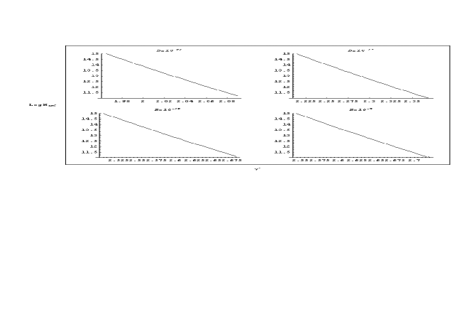
Figure 1: $Log(H_{inf})$ relative to $\nu^{\prime}$, for magnetic fields with strengths $10^{-23}$, $10^{-17}$, $10^{-10}$G on 1 MPc scale and $10^{-9}$G on 10 MPc scale, at present.

To find a range for $\nu^{\prime}$ variations, the graph of $\log(H_{inf})$ with respect to $|\nu^{\prime}|$ is plotted (fig. LABEL:Fig1). By taking the logarithm of both sides, one has

$$Log(H_{inf})={(\frac{2~{}\nu^{\prime}-1}{2})}^{-1}(-(16.041(2~{}\nu^{\prime}-5)$$

$$+2~{}Log(\Gamma(\nu^{\prime})+0.6~{}\nu^{\prime})+51.98-2Log|\vec{B}|)\;.$$ (67)

As mentioned before, the upper limit for $H_{inf}$ is $2.4\times 10^{-14}GeV$. We can estimate a lower limit for $H_{inf}$ by noting that duration of the inflationary stage had been about $10^{-34}$ [22] and that the least value of e-folding number should be about $60$

$$\frac{a_{i}}{a_{R}}=e^{N}=e^{\Delta t~{}H}~{}~{}~{}~{}~{}~{}~{}\Rightarrow~{}~{}~{}~{}~{}~{}~{}H_{inf}=(\Delta t)^{-1}N=4\times 10^{11}GeV\;.\\$$ (68)

where ”i” means value of quantities at the beginning of inflation. Now, we use Eq.(67) to depict the graph of $\log(H_{inf})$ versus $|\nu^{\prime}|$, for the magnetic fields with strengths $10^{-23}$, $10^{-17}$, and $10^{-10}$ G on $1$ Mpc scale (galaxies) and $10^{-9}$ G on $10$ Mpc scale (cluster of galaxies). From Fig. (1), we find that for the magnetic fields mentioned, with $10^{11}<H_{inf}<10^{15}$, the ranges of $\nu^{\prime}$ variations are $1.96<\nu^{\prime}<2.9$, $2.21<\nu^{\prime}<2.37$, $2.5<\nu^{\prime}<2.68$ and $2.54<\nu^{\prime}<2.75$, respectively. All of these ranges violate the consistency condition, $|\nu^{\prime}|<\frac{3}{2}$. From Eqs.(57)-(60), it can be seen that the consistency condition comes from $H_{\nu^{\prime}+1}^{(1)}(\frac{k}{aH_{inf}})$ (which is part of the electric field). For solving this problem, we have to cancel out the term $H_{\nu^{\prime}+1}^{(1)}$. Imposing the condition $\nu-\frac{1}{2}=\nu^{\prime}$ on eq.(3) and considering the following relations between derivations of Hankel functions

$$H_{\nu^{\prime}-1}^{(1)}(x)+H_{\nu^{\prime}+1}^{(1)}(x)=2\frac{\nu^{\prime}}{x}H_{\nu^{\prime}}^{(1)}(x)$$

$$H_{\nu^{\prime}-1}^{(1)}(x)-H_{\nu^{\prime}+1}^{(1)}(x)=2\frac{d}{dx}H_{\nu^{\prime}}^{(1)}(x)\;.$$ (69)

the electric field can be written as

$${E_{I}}^{C}(k,a)=\sqrt{\frac{\pi}{4H_{inf}f(a)}}\hskip 3.41432pt\left(\frac{k}{a}\right)a^{-1/2}\left(\frac{k}{aH_{inf}}\right)H_{\nu^{\prime}-1}^{(1)}e^{i(\nu^{\prime}+1)\pi/4}\;.$$ (70)

Now rewriting eqs.(57)-(60) using the above relation, we arrive at

$$\Theta\approx\frac{1}{9\pi^{2}w}{\left(\frac{H_{inf}}{M_{Pl}}\right)}^{2}x^{-5+2\nu^{\prime}}(2^{2\nu^{\prime}}\Gamma^{2}(\nu^{\prime})+2^{2(\nu^{\prime}-1)}\Gamma^{2}(\nu^{\prime}-1)x^{-2})~{}~{}~{}~{}~{}~{}~{}~{}~{}~{}~{}~{}~{}\nu^{\prime}>1\;,$$ (71)

$$\Theta\approx\frac{1}{9\pi^{2}w}{\left(\frac{H_{inf}}{M_{Pl}}\right)}^{2}x^{-5+2\nu^{\prime}}(2^{2\nu^{\prime}}\Gamma^{2}(\nu^{\prime})+2^{2(\nu^{\prime}-1)}\Gamma^{2}(\nu^{\prime}-1)x^{-2})~{}~{}~{}~{}~{}~{}~{}~{}0<\nu^{\prime}<1\;,$$ (72)

$$\Theta\approx\frac{1}{9\pi^{2}w}{\left(\frac{H_{inf}}{M_{Pl}}\right)}^{2}x^{-(5+2\nu^{\prime})}(2^{-2\nu^{\prime}}\Gamma^{2}(-\nu^{\prime})+2^{-2(\nu^{\prime}+1)}\Gamma^{2}(-\nu^{\prime}-1)x^{-2})~{}~{}~{}\nu^{\prime}<-1\;.$$ (73)

The new consistency condition is $\frac{-3}{2}<\nu^{\prime}<\frac{5}{2}$. The problem of satisfying the consistency condition still remains for $\nu^{\prime}>\frac{-3}{2}$ and, therefore, the acceptable range for $\nu^{\prime}$ variation is $\nu^{\prime}<\frac{5}{2}$. The new consistency condition is derived by the redefinition of $\nu-\frac{1}{2}=\nu^{\prime}$ while we have $\alpha=\nu$ from Eq.(31) which results in a new consistency condition as $\alpha<3$. Using $\nu^{\prime}=\alpha-\frac{1}{2}$ in Eqs.(59) and (67) one has

$$\frac{1}{2}\times 4.8\times 10^{-39}~{}B(L,t_{0})^{2}=\frac{2^{2\alpha-4}}{3\pi^{2}}~{}\Gamma^{2}(\alpha-1/2){(\frac{g_{*}}{3.91})}^{-1/3}\times 1.66~{}~{}T_{\gamma_{0}}(GeV)$$

$$\times~{}{g_{*}}^{1/2}(~{}{\sqrt{\frac{H_{inf}}{M_{Pl}}}~{}})^{4}\times{(~{}(\frac{(\frac{30}{{\pi}^{2}g_{*}})^{-1/6}}{10^{38/3}[GeV][Mpc]}\sqrt{H_{inf}M_{Pl}}L~{}[Mpc])\times e^{45})}^{2\alpha-6}\;.$$ (74)

$$Log(H_{inf})={(\alpha-1)}^{-1}(-(16.041(2~{}\alpha-6)+2~{}Log(\Gamma(\alpha-1/2))$$

$$~{}~{}~{}~{}~{}~{}~{}~{}~{}~{}+0.6(~{}\alpha-1/2))+51.98-2Log|\vec{B}|)\;.$$ (75)

We conclude from Eq.(75) that the larger $H_{inf}$ and $\alpha$, the larger will the magnetic field be. For $\alpha=1$, magnetic field is $2.1\times 10^{-58}$ G in $1$ Mpc scale which is independent of $H_{inf}$. For $\alpha=3$, magnetic field spectrum is invariant, and the maximum value of the field is $1.8\times 10^{-11}$ G for $H_{inf}=2.4\times 10^{14}GeV$. By using Eq.(75) to depict the graph of $\log(H_{inf})$ versus $|\nu^{\prime}|$, for the magnetic fields with strengths $10^{-23}$, $10^{-17}$ and $10^{-10}$ G on $1$ Mpc scale (galaxies) and $10^{-9}$ G on $10$ Mpc scale (cluster of galaxies), Fig. (2), it is clear that for $10^{-23}$ G and $10^{-17}$ G fields, the consistency condition holds in the appropriate range for $H_{inf}$ while it does not for $10^{-10}$ G and $10^{-9}$ G fields. This should not concern us since we got $10^{-10}$ G and $10^{-9}$ G fields by assuming that the galactic dynamo does not act on galactic scales which is not, indeed, realistic.

As mentioned before, the most real situation for galaxies is a $10^{-17}$G magnetic field on $1$ Mpc scale, which transforms to a $10^{-6}$G field observed today via gravitational collapse and dynamo action. In this way, a range for $\alpha$ parameter can be obtained

$$2.71<\alpha<2.8\;.\\$$ (76)

Therefore, when dilaton freezes after inflation, the best range for the coupling $f(\Phi)$ can be determined from eq.(76). Considering $f=f_{0}a^{2\alpha-2}$, $a=c~{}t^{1/2}$ (c is a constant) , $f(t_{R})=1$ and $t_{R}\approx\frac{1}{2H_{inf}}$, we have

$$f_{0}=c^{*}~{}(2H_{inf})^{\alpha-1}\;.$$

Obtaining the value for $f_{0}$ and having the range of $\alpha$, we can determine the dilaton coupling in this case.

From Eq.(31) and the consistency condition that leads to $\nu^{\prime}=\nu-1/2=\alpha-1/2$, we get

$$\xi=\frac{\alpha-1/4}{24}\;.$$ (77)

and from Eq.(70), we have $\xi\simeq\frac{1.23}{12}$ that is close to the value $\frac{1}{12}$, as derived by Turner and Widrow in [5]. Since $\alpha$ and $\xi$ parameters are specified, the coupling to electromagnetic field for generating the $10^{-17}G$ magnetic field is determined.

Conventionally, $\xi$ is a constant parameter [5] and the term $\xi RA^{2}$ will become very small after inflation since Ricci scalar in FRW metric is: $R=\frac{{\ddot{a}}a+{\dot{a}}^{2}+K}{a^{2}}$ and it will be very small in the radiation and matter dominated epoch, hence it will be removed.

6 Dilaton decay

By now, we have assumed that the dilaton evolution ends after inflation. Let us now consider a more realistic situation (like in [13]) in which the dilaton continues its evolution and reaches its minimum potential, then it begins to oscillate and then decays (the dilaton evolves from $\Phi_{R}(<0)$ to its minimum in $\Phi=0$ and here, $f=1$).

6.1 Dilaton evolution after inflationary stage

During coherent oscillation, the energy density $\rho_{\Phi}$, of the dilaton field evolves as $a^{-3}$ which is slower than the energy density of radiation produced by the inflaton field via its decay, $\rho_{\phi}$. If the condition $\rho_{\Phi}<\rho_{r}$ holds until dilaton decays, the entropy per comoving volume remains approximately unchanged, but if it changes to $\rho_{\Phi}>\rho_{r}$, a large amount of entropy will be produced [12]. If this happens, the magnetic energy density will be diluted by entropy production.

We consider $t_{osc}\simeq m^{-1}$ ($m$ is dilaton mass) as the time when coherent oscillations begin. When $t>t_{R}$, the universe is radiation dominated and thus, $a(t)=a_{R}(t/t_{R})^{1/2}$. Before coherent oscillation, $t_{R}<t<t_{osc}$, the dilaton field evolves with its exponential potential.

The amplitude of the dilaton field, $\Phi_{R}$, is relatively small at the end of inflation. This is a consequence of the condition we imposed on the magnetic field energy density (consistency condition). When $t_{R}<t<t_{osc}$, the magnetic energy density increases by the dilaton evolution. The magnetic energy density should be smaller than the dilaton one on all scales so that it does not affect the dilaton evolution. As will be shown, larger values of $\bar{\lambda}\kappa|\Phi_{R}|$ result in larger values of the magnetic energy density and, thus, we get an upper limit for $\bar{\lambda}\kappa|\Phi_{R}|$ from here. By solving the dilaton equation of motion with exponential potential (eq.(10)) numerically, we get a range for $\bar{\lambda}\kappa|\Phi_{R}|$ that satisfies these conditions [13]. The result is that $|\Phi_{R}|$ with $\bar{\lambda}\sim{\cal O}(1)$ should be of the order $1/\kappa$.

With these conditions and the fact that $\bar{V}\exp(-\bar{\lambda}\kappa\Phi_{R})/\rho_{\phi}$ $\approx\omega\ll 1$, the dilaton energy density will not be larger than the radiation energy density and we will, therefore, have entropy production only in the coherent oscillation epoch, $t\sim t_{osc}$. By considering the slow roll condition, we have $\rho_{\Phi}\approx V[\Phi]$ for the dilaton field. The dilaton gets its minimum of potential at $t_{osc}$ and thus, $\rho_{\Phi}\approx\bar{V}$. The minimum arises when other contributions from gaugino condensation enter into the to dilaton potential and generate a minimum [13]. If the universe stays radiation-dominated while the dilaton decays, $t_{d}\simeq\Gamma_{\Phi}^{-1}$, then

$${{\rho}_{r}}^{(inf)}(t_{\Phi})>{\rho}_{\Phi}(t_{\Phi})$$ (78)

or

$${\rho}_{\phi}[\frac{a(t_{\Phi})}{a_{R}}]^{-4}>{\rho}_{\Phi}(t_{osc})[\frac{a(t_{\Phi})}{a(t_{osc})}]^{-3}$$ (79)

Since, $\rho_{\Phi}\approx\bar{V}$, one gets

$$\frac{{\rho}_{\phi}}{\bar{V}}>\left(\frac{M_{Pl}}{m}\right)\left(\frac{2H_{inf}}{m}\right)^{2}\;.$$ (80)

where, we have used $\Gamma_{\Phi}\simeq m(m/M_{pl})^{2}$ and $t_{R}\approx\frac{1}{2}H_{inf}$. Entropy per comoving volume remains constant here [12].Thus, the necessary condition for entropy production is

$$\frac{{\rho}_{\phi}}{\bar{V}}<\left(\frac{M_{Pl}}{m}\right)\left(\frac{2H_{{inf}}}{m}\right)^{2}\;.$$ (81)

Suppose the dilaton energy density equals radiation energy density at $t=t_{c}$

$${\rho}_{\phi}[\frac{a(t_{c})}{a_{R}}]^{-4}={\rho}_{\Phi}(t_{{osc}})[\frac{a(t_{c})}{a(t_{osc})}]^{-3}\;.$$ (82)

We, therefore, have

$$t_{c}\approx(\frac{{\rho}_{\phi}}{\bar{V}})^{2}{t_{R}}^{4}\hskip 0.56905pt{t_{{osc}}}^{-3}\approx\left(\frac{{\rho}_{\phi}}{\bar{V}}\right)^{2}\left(\frac{1}{2H_{{inf}}}\right)^{4}m^{3}\;.$$ (83)

where $\rho_{\Phi}(t_{osc})\approx\bar{V}$ and $t_{osc}\simeq$ $m^{-1}$ are assumed. After $t_{c}$, $\rho_{\Phi}$ dominates over $\rho_{R}$ and universe becomes matter-dominated and thus $a(t)=a_{c}(t/t_{c})^{2/3}=a_{R}t_{R}^{-\frac{1}{2}}t_{c}^{-\frac{1}{6}}t^{\frac{2}{3}}$ that second equality comes from continuity condition of $a(t)$ at $t=t_{R}$.

The entropy per comoving volume is $S=a^{3}(\rho+p)/T$ where $\rho$, $p$ and T are energy density, pressure, and temperature, respectively, in equilibrium [12] and we have

$$S^{4/3}={S_{c}}^{4/3}+\hskip 2.84526pt\frac{4}{3}{\rho}_{\Phi}(t_{c}){a_{c}}^{4}[\frac{2{\pi}^{2}\langle g_{*}\rangle}{45}]^{1/3}{\Gamma}_{\Phi}\int_{t_{c}}^{t}[\frac{a(\tau)}{a_{c}}]\exp[\hskip 1.42262pt-{\Gamma}_{\Phi}(\tau-t_{{c}})\hskip 1.42262pt]d\tau\;,$$

$${S_{c}}^{4/3}[\hskip 1.42262pt1+{\Gamma}_{\Phi}{t_{c}}^{-2/3}\int_{0}^{\infty}(u+t_{{c}})^{2/3}\exp(-{\Gamma}_{\Phi}u)du\hskip 1.42262pt]\approx{S_{c}}^{4/3}[\hskip 1.42262pt1+\Gamma(\frac{5}{3})(t_{{c}}{\Gamma}_{\Phi})^{-2/3}\hskip 1.42262pt]\;.$$ (84)

where $S_{c}$ is the entropy per comoving volume at $t_{c}$ and $<g_{*}>$ is the average of $g_{*}$ (number of degrees of freedom ) for decay duration. In the second approximation, we have $u\equiv\tau-t_{c}$ and we consider the limit $u\rightarrow\infty$. In addition, we have used $\rho_{r}(t_{c})=\rho_{\Phi}(t_{c})$ and the following equation

$$S=[\hskip 2.84526pt\frac{4}{3}(\frac{2{\pi}^{2}g_{*}}{45})^{1/3}a^{4}{\rho}_{{r}}\hskip 2.84526pt]^{3/4}\;.$$ (85)

that in general, gives the relation between the radiation energy density and the entropy per comoving volume. From $\Gamma_{\Phi}\simeq m(m/M_{pl})^{2}$ and Eqs.(83) and (84), we find that the ratio of entropy per comoving volume after decay to that of before decay is written as:

$$\Delta S\equiv\frac{S}{S_{c}}\\ \approx\{\hskip 2.84526pt1+\Gamma(\frac{5}{3})[\left(\frac{\bar{V}}{{\rho}_{\phi}}\right)\left(\frac{2H_{{inf}}}{m}\right)^{2}\left(\frac{M_{Pl}}{m}\right)]^{4/3}\hskip 2.84526pt\}^{3/4}\\ \approx\left(\frac{\bar{V}}{{\rho}_{\phi}}\right)\left(\frac{2H_{{inf}}}{m}\right)^{2}\left(\frac{M_{Pl}}{m}\right)\;.$$

By entropy production, the universe expands more rapidly to cancel this entropy production. It follows from this observation and also from the relation $\rho_{r}\propto a^{-4}S^{4/3}$, that

$$(\Delta S)^{4/3}=\left(\frac{{a_{0}}^{\prime}}{a_{0}}\right)^{4}\;.$$ (86)

where ${a_{0}}^{\prime}$ is the present scale factor when we have entropy production.

Finally, we investigate the effect of dilaton decay on the energy density of present large scale magnetic fields. Again, we assume that the universe immediately becomes highly conductive after reheating. From Eqs.(52),(6.1), and (86), we find the ratio of magnetic field energy density at the present time, when dilaton continues evolving after reheating, $\rho^{\prime}$, to the situation that dilaton freezes in the reheating, $\rho$, is

$$\frac{\rho^{\prime}}{\rho}=f^{-1}(t_{R})(\Delta S)^{-4/3}\;,\\$$

We define

$$\omega=\frac{V[\Phi]}{\rho_{\phi}}$$ (87)

Since we assumed $\rho_{\phi}>>\rho_{\Phi}$, then $\omega<<1$ which we consider as $\omega\approx 10^{-2}$.

From Eq.(6.1) and $\frac{\bar{V}}{\rho_{\phi}}\approx\omega exp~{}(\bar{\lambda}\kappa\Phi_{R})$, we arrive at

$$\frac{\rho^{\prime}}{\rho}\approx f^{-1}(t_{R})\exp[\hskip 1.42262pt\frac{4}{3}~{}\bar{{\lambda}}\kappa{\Phi}_{R}\hskip 1.42262pt][\hskip 2.84526ptw(\frac{2H_{{inf}}}{m})^{2}(\frac{M_{Pl}}{m})\hskip 2.84526pt]^{-4/3}\;.$$ (88)

As can be seen from RHS of the above equation, it is the dilaton coupling that increases $\rho^{\prime}$ relative to $\rho$.

6.2 Magnetic fields with dilaton decay

Considering $f=f_{0}a^{2\alpha-2}$, $a=c~{}t^{1/2}$ (c is a constant), $f(t_{osc})=1$ and $t_{osc}\approx\frac{1}{m}$, we have

$$f_{0}=c^{*}~{}m^{\alpha-1}\;.$$

since $t_{R}=\frac{1}{2H_{inf}}$,

$$f(t_{R})=m^{\alpha-1}~{}({2H_{inf}})^{1-\alpha}\;.$$ (89)

We estimate from Eqs.(52), (88) and (89), the present strength of magnetic fields for the case in which dilaton continues evolving after reheating which leads to the following relation:

$$Log(B^{\prime}(t_{0}))=\frac{1}{2}[{(\alpha-1)}Log(H_{inf})+c(2~{}\alpha-6)+2~{}Log(\Gamma(\alpha-1/2)$$

$$+0.6(~{}\alpha-1/2))-23.96+\bar{\lambda}\kappa|\Phi_{R}|+(\alpha-1)(Log(2H_{inf})-Log(m))+\Delta S]\;.$$ (90)

c is equal to $16.041$ and $17.041$ on $1$ Mpc and $10$ Mpc scale, respectively. It can be seen that a stronger magnetic field results from a larger value of $\bar{\lambda}\kappa|\Phi_{R}|$. As said before, $\bar{\lambda}\kappa|\Phi_{R}|$ is of the order $1$ and any bigger value violates the consistency condition. Therefore, we use the maximum possible value for $\bar{\lambda}\kappa|\Phi_{R}|(=1)$ and plot the graph for $Log(B^{\prime})$ versus $\alpha$ (fig(3)). The graphs of magnetic field strengths are on $10$ Mpc scale in ”A” and ”B” and on $1$ Mpc scale in ”C” and ”D”. We have entropy production in all the cases. The entropy production in ”B”, ”D”, and ”F” is $4.4\times 10^{9}$ while it is about $2\times 10^{5}$ in ”A”, ”C”, and ”E”.

Comparing these graphs with those of Fig(2), one can find that in this case smaller values of $\alpha$ give the desired magnetic fields $(10^{-23},10^{-17},10^{-10}~{}and~{}10^{-9}G)$ and we don’t have consistency condition violation in any of the field strengths.

The graphs ”E” and ”F” represent a strength of $10^{-17}$ (which is the best choice ) with $H_{inf}=10^{14}~{}Gev$ and $H_{inf}=10^{11}~{}Gev$, respectively.

From graphs ”E” and ”F”, the best range for $\alpha$ to give the acceptable strength is $2.215<\alpha<2.441$ and when the value of $\xi$ is obtained from Eq.(70), the couplings are completely determined.

7 conclusion

In this work, a mechanism is introduced for amplifying quantum fluctuations in the inflationary universe and for producing large scale magnetic fields. This is accomplished by breaking the conformal invariance of electromagnetic theory in the early universe by coupling the gravity (curvature of spacetime) and a scalar field (dilaton) to it. These couplings have been studied separately, before. Here, the more realistic problem to the effect that both of these couplings exist together is considered.

Two different situations have been discussed for the evolution of the dilaton scalar field. In the first situation, whereby the dilaton is assumed to freeze at the end of inflation, the parameters of the model are determined for the seed magnetic field that gives the presently observed strengths by the effect of amplification mechanisms. By considering the strength of $10^{-17}$ gauss as the best value for the seed magnetic field to give presently observed field, we fixed our coupling parameters as : $2.71<\alpha<2.8$ (we use ”2.71” that corresponds to the upper limit of $H_{inf}$ which is more realistic) and $\xi\approx\frac{1.23}{12}$.

In the second situation, which assumes that the dilaton continues its evolution after the inflation, a large amount of entropy can be produced that dilutes the energy density of the magnetic fields produced. Here, we expect less values for $\alpha$ since our coupling nears unity in a larger time than the previous case. The range for variations of the parameters that give the desired magnetic field ( $10^{-17}$ gauss ) includes $2.215<\alpha<2.441$ and $\xi\approx\frac{0.98}{12}$ which is closer to the value derived in [5].

Acknowledgements

We would like to thank Prof. B.Ratra, Dr. K.Bamba and Dr. N.Afshordi for their useful discussion and suggestions and Isfahan University of Technology for their financial support.

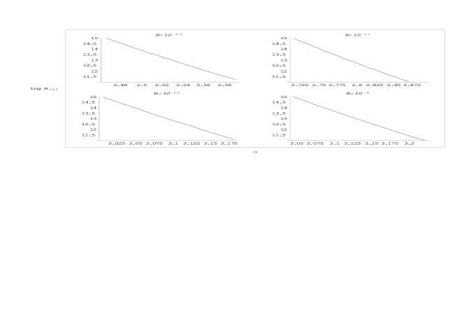
Figure 2: $Log(H_{inf})$ relative to $\alpha$, for magnetic fields with strengths $10^{-23}$, $10^{-17}$, $10^{-10}$G on 1 MPc scale and $10^{-9}$G on 10 MPc scale, at present

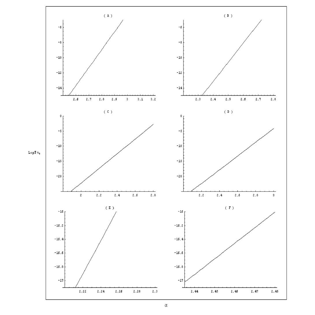
Figure 3: $Log(B^{\prime}(T_{0}))$ relative to $\alpha$, for $H_{inf}=2.4\times 10^{14}GeV$, $m=2.4\times 10^{13}GeV$ in ”A”, ”C” and ”E”, for $H_{inf}=10^{11}$GeV, $m=10^{10}$GeV in ”B”, ”D” and ”F”. Graphs ”A” and ”B” are on 10 Mpc and others are on 1 Mpc. Graphs ”E” and ”F” are depicted to get the accurate value of $\alpha$.

References

- [1] P. P. Kronberg, Rep. Prog. Phys. 57, 325 (1994).
- [2] K. Enqvist, Int. J. Mod. Phys. D, 7, 331 (1998); D.Grasso and H. Rubinstein, Phys. Rep., 348, 163 (2001); L Widrow, Rev. Mod. Phys., 74, 775 (2002); M. Giovannini, Int. J. Mod. Phys. D, 13, 391 (2004).
- [3] L. M. Widrow, Rev. Mod. Phys. 74, 775 (2002).
- [4] Dolgov, A. D. “Generation of Magnetic Fields in Cosmology ”, hep-ph/0110293.
- [5] M.S. Turner, L.M. Widrow, Phys. Rev., D 37 (1988) 2743.
- [6] B. Ratra, Astrophys. J., 391 (1992) L1.
- [7] A.D. Dolgov, Phys. Rev., D 48 (1993) 2499.
- [8] C.H. Hogan, Phys. Rev. Lett., 51 (1983) 1488.
- [9] T. Vachaspati, A. Vilenkin, Phys. Rev. Lett., 67 (1991) 1057.
- [10] A.D. Dolgov, J. Silk, Phys.Rev., D 47 (1993) 3144.
- [11] A.D. Dolgov, D. Grasso, astro-ph/0106154.
- [12] E. W. Kolb, M. S. Turner,“ The Early Universe” (Addison Wesley, New York, 1989).
- [13] K. Bamba, J. Yokoyama, Phys. Rev., D 69 (2004) 043507, astro-ph/0310824; Phys. Rev., D 70 (2004) 083508, hep-ph/0409237.
- [14] K. Bamba, Private communication.
- [15] M. Chanowitz, J. Ellis, Phys. Rev., D7 (1973) 2490.
- [16] M. Giovannini, hep-ph/0104214.
- [17] B. Rartra, Inflation Generated Cosmological Magnetic Fields, GRP-287/CALT-68-1751 (1991).
- [18] M. Giovannini,” The Magnetizd Universe ”, astro-ph/0312614.
- [19] V. A. Rubakov, M. V. Sazhin, and A. V. Veryaskin, Phys. Lett. 115B, 189 (1982).
- [20] L. F. Abbott and M. B. Wise, Nucl. Phys. B244, 541 (1984).
- [21] D. N. Spergel et al., Astrophys. J., Suppl. 148, 175 (2003).
- [22] M. Roos, Introduction to Cosmology WILEY, (1997).
- [23] E. N. Parker, ”Cosmical Magnetic Fields”, Claron, Oxford, England, 1979.
- [24] Ya. B. Zel’dovich, A. A. Ruzmaikin and D. D. Sokollof, ”Magnetic Fields in Astrophysivs”, Gordon and Breach, New York, 1983.