MIFP-07-17

MCTP-07-20

UCI-TR-2007-30

Probing the Green-Schwarz Mechanism
at the Large Hadron Collider

Jason Kumar¹, Arvind Rajaraman², James D. Wells^3
(1)Department of Physics, Texas A&M University, College Station, TX 77843-4242, USA
⁽²⁾Department of Physics, University of California, Irvine, CA 92697, USA
⁽³⁾Michigan Center for Theoretical Physics (MCTP)
Department of Physics, University of Michigan, Ann Arbor, MI 48109, USA

We investigate the phenomenology of new abelian gauge bosons, which we denote as $X$ bosons, that suffer a mixed anomaly with the Standard Model, but are made self-consistent by the Green-Schwarz mechanism. A distinguishing aspect of the resulting effective theory is the decay of $X$ bosons into Standard Model gauge bosons, $X\to ZZ,WW,\gamma Z$. We compute the production cross-section of the $X$ boson from vector boson fusion at the Large Hadron Collider. We study the $pp\to X\to ZZ\to 4l$ signal, and analyze the prospects of discovery. We argue that such a discovery could indirectly probe high energies, even up to the string scale.

July 2007

Introduction

Many of the most well-motivated ideas for physics beyond the Standard Model (SM) suggest the existence of new $U(1)$ gauge bosons. Such gauge bosons occur naturally in $SO(10)$ grand unified models, extra dimensional models with a hidden sector brane, and string theoretic models with intersecting branes. If these gauge bosons are coupled to leptons, they can provide spectacular and clean signals at colliders.

However, in many models, there need not be a tree-level coupling between the SM particles and the new $U(1)$ gauge bosons. In particular, SM-like intersecting brane model (IBM) constructions [1, 2] typically contain relatively large gauge groups of which the SM is only one sector. In these models, the SM fermions typically have no couplings to the other gauge groups.

In these models, couplings to the hidden sector can be generated at the loop level. Kinetic mixing can give rise to couplings of the hidden-sector gauge bosons to SM states. The quantum corrections that mix the kinetic terms of the extra gauge boson and hypercharge are unsuppressed by any mass scales, yielding renormalizable terms that probe both the ultraviolet (UV) scales and infrared (IR) scales [3].

In this letter we will study a different limit, where the couplings are dominated by terms from a mixed anomaly (the consistency of which will be made clear below) between the SM gauge sector and an exotic $U(1)_{X}$. In this circumstance, we will have a massive hidden sector gauge boson $X$ whose main couplings to the SM sector are through the gauge fields. Such a gauge boson can have distinctive signatures at colliders.

These anomaly terms are of great interest for another reason: they could indirectly probe high energy physics, and possibly even stringy effects. This is because anomalies can be thought of as both UV and IR effects. They are clearly visible in the limit of low-energy effective field theory which we expect to match to data, yet their UV character implies that the existence (and resolution) of these anomalies can often be tied to a stringy origin. This stringy origin also implies that in a wide variety of models, the same types of anomaly effects can be observed, thus making the anomaly an interesting candidate for a stringy signature to be observed at colliders.

Gauge anomalies must be cancelled for consistency. In string theory this is achieved via the Green-Schwarz mechanism, wherein closed string couplings yield classical gauge-variant terms whose variation cancels the anomalous diagrams. This mechanism can have phenomenological consequences [4, 5, 6, 7], and observable effects at the Large Hadron Collider (LHC). In particular, we will find that the measurement of these anomalous couplings can probe the non-vectorlike couplings of the entire Hagedorn tower of states that arise in IBM’s.

Below, we first review the intersecting brane model setup that gives motivation to the mixed anomaly couplings of SM gauge bosons with an exotic $X$ gauge boson. We then calculate the effective vertex that couples the hidden sector $X$ gauge boson to the visible sector. We will consider the phenomenology of this generic IBM setup by identifying a simple effective theory description that obviates the need to further consider the string theory origin. After having the effective theory description in place, we compute the decay widths for the hidden sector gauge boson, and use the results to compute the cross-section for production of $X$ via vector boson fusion. We outline the parameter space that can be probed by the LHC in the clean four lepton final state mode. We conclude with a short discussion of our results.

Intersecting Brane Models and the Effective Theory

Consider IBM’s arising from Type IIA string theory compactified on an orientifolded CY 3-fold. The branes in question are spacetime-filling D6-branes wrapping 3-cycles of the Calabi-Yau. The SM arises from strings that begin and end on a certain set of D-branes (the so-called “visible” sector branes). Additional D-branes are generally required in order to cancel RR-tadpoles, or, equivalently, to ensure that all space-filling charges cancel. These additional D-branes generate gauge groups beyond the SM (the “hidden” sector).

Chiral matter arises from strings stretching between two different branes or their orientifold images. For example, if $a$ and $b$ are two stacks of branes with gauge groups $G_{a}$ and $G_{b}$ living on them, the net number of chiral multiplets charged under the bifundamental of these two groups is counted by the topological intersection number of these branes, $I_{ab}$. In particular, if hidden sector branes have non-trivial topological intersection with visible sector branes, there will be a net number of chiral multiplets transforming in the bifundamental of SM and hidden sector gauge groups. Note that these topological intersection numbers are generically nonzero, as any two 3-cycles will generally intersect on a 6-manifold.

Consider a hidden sector with a diagonal subgroup $U(1)_{X}$. Generically, there will be a non-zero number of chiral multiplets in the bifundamental of this group and the SM group $SU(2)_{L}$. These chiral multiplets will lead to a $[U(1)_{X}SU(2)_{L}^{2}]$ mixed anomaly through triangle diagrams with fermions running in the loop. This anomaly will be cancelled by the Green-Schwarz mechanism, which arises from adding to the Lagrangian terms that are classically gauge-variant, and whose gauge variation cancels the anomalous triangle diagrams. There will be two types of such terms: a generalized Chern-Simons term which couples the gauge boson of $U(1)_{X}$ to the $SU(2)_{L}$ gauge bosons, and a Peccei-Quinn term which couples the $SU(2)_{L}$ field strength to an axion. We may write the Lagrangian as the sum of classically gauge-invariant and gauge-variant pieces [5] as

$$L_{inv.} = -{1\over 2}Tr[F_{W}^{2}]-{1\over 2}(\partial_{\mu}a+M_{X}X_{\mu})^{2}-\bar{\psi}\gamma^{\mu}D_{\mu}\psi$$

$$L_{var.} = {D^{\prime}\over 24\pi^{2}}a\,Tr\,F_{W}\wedge F_{W}+{Z\over 48\pi^{2}}\epsilon^{\mu\nu\rho\sigma}X_{\mu}\Omega_{\nu\rho\sigma}$$ (1)

where ${1\over 2}\partial_{\mu}\Omega_{\nu\rho\sigma}=Tr[F_{W}\wedge F_{W}]$ and the axion has a shift transformation under $U(1)_{X}$ of $a\rightarrow a+M_{X}\lambda$. In a string theory setting, the Green-Schwarz mechanism arises automatically. In the UV limit of the one-loop open string diagram, the annulus stretches into a closed string which couples at tree-level to the open strings. One can also consider the example of a $U(1)_{X}$ arising in the SM sector [8].

These new gauge-variant terms will also contribute to an effective vertex for a coupling between the $U(1)_{X}$ gauge boson and two $SU(2)_{L}$ gauge bosons[5, 6]. For a suitable choice of coefficients $D^{\prime}$ and $Z$, the anomalous terms can be cancelled, and the resulting theory satisfies the Ward identity.

Although the divergences and anomaly are cancelled, the triangle diagram nevertheless contributes an unambiguous finite piece to the effective vertex operator for an interaction between a $U(1)_{X}$ gauge boson and two $SU(2)_{L}$ vector bosons. Following [5], we can write this effective vertex as

$$\Gamma_{\mu\nu\rho}^{\alpha}(k_{3}^{X},k_{1}^{Z},k_{2}^{Z}) = t^{\alpha}[A_{1}\epsilon_{\mu\nu\rho\sigma}k_{2}^{\sigma}+A_{2}\epsilon_{\mu\nu\rho\sigma}k_{1}^{\sigma}+B_{1}k_{2\nu}\epsilon_{\mu\rho\sigma\tau}k_{2}^{\sigma}k_{1}^{\tau}+B_{2}k_{1\nu}\epsilon_{\mu\rho\sigma\tau}k_{2}^{\sigma}k_{1}^{\tau}$$ (2)

$$+B_{3}k_{2\rho}\epsilon_{\mu\nu\sigma\tau}k_{2}^{\sigma}k_{1}^{\tau}+B_{4}k_{1\rho}\epsilon_{\mu\nu\sigma\tau}k_{2}^{\sigma}k_{1}^{\tau}$$

$$+D{k_{3\mu}\over k_{3}^{2}}\epsilon_{\nu\rho\sigma\tau}k_{2}^{\sigma}k_{1}^{\tau}+Z\epsilon_{\mu\nu\rho\sigma}(k_{2}^{\sigma}-k_{1}^{\sigma})]$$

In this expression, $Z$ arises from the generalized Chern-Simons terms and $D$ arises from the Peccei-Quinn terms and from the one-loop coupling of the fermions to the Goldstone boson (computed in Lorentz gauge). $A_{1,2}$ and $B_{1,2,3,4}$ are the coefficients of tensor structures which arise from computation of the triangle diagrams with three gauge bosons as external legs. $B_{1,2,3,4}$ are finite and unambiguously determined by the triangle diagrams [5],

$$B_{1}(k_{1},k_{2})=-B_{4}(k_{2},k_{1}) = -{\imath g_{h}g_{W}^{2}\over 8\pi^{2}}\sum_{i}t_{i}\int_{0}^{1}d\alpha d\beta{2\alpha\beta\over\alpha k_{2}^{2}+\beta k_{1}^{2}-(\alpha k_{2}-\beta k_{1})^{2}-m_{i}^{2}}$$

$$B_{2}(k_{1},k_{2})=-B_{3}(k_{2},k_{1}) = -{\imath g_{h}g_{W}^{2}\over 8\pi^{2}}\sum_{i}t_{i}\int_{0}^{1}d\alpha d\beta{2\beta(1-\beta)\over\alpha k_{2}^{2}+\beta k_{1}^{2}-(\alpha k_{2}-\beta k_{1})^{2}-m_{i}^{2}}$$ (3)

where $g_{h}$ is the gauge coupling of the hidden sector $U(1)_{X}$, $g_{W}$ is the gauge coupling of $SU(2)_{L}$ and $t_{i}$ encode the charges of the fields in the loop. $A_{1,2}$ are UV cutoff dependent coefficients which depend on how the diagram is regulated. Since we have used Lorentz gauge, the Ward identity takes a simple form:

$$\epsilon_{3}^{\mu}k_{1}^{\nu}\epsilon_{2}^{\rho}\Gamma_{\mu\nu\rho}=\epsilon_{3}^{\mu}\epsilon_{1}^{\nu}k_{2}^{\rho}\Gamma_{\mu\nu\rho}=k_{3}^{\mu}\epsilon_{1}^{\nu}\epsilon_{2}^{\rho}\Gamma_{\mu\nu\rho}=0$$ (4)

where $k_{1}+k_{2}+k_{3}=0$. We can remove the divergences in the $A_{1,2}$ coefficients and fix the ambiguity by the redefinition $\tilde{A}_{1}=A_{1}+Z$, $\tilde{A}_{2}=A_{2}-Z$, yielding

$$\Gamma_{\mu\nu\rho}^{\alpha}(k_{3}^{X},k_{1}^{W},k_{2}^{W}) = t^{\alpha}[\tilde{A}_{1}\epsilon_{\mu\nu\rho\sigma}k_{2}^{\sigma}+\tilde{A}_{2}\epsilon_{\mu\nu\rho\sigma}k_{1}^{\sigma}+B_{1}k_{2\nu}\epsilon_{\mu\rho\sigma\tau}k_{2}^{\sigma}k_{1}^{\tau}+B_{2}k_{1\nu}\epsilon_{\mu\rho\sigma\tau}k_{2}^{\sigma}k_{1}^{\tau}$$ (5)

$$+B_{3}k_{2\rho}\epsilon_{\mu\nu\sigma\tau}k_{2}^{\sigma}k_{1}^{\tau}+B_{4}k_{1\rho}\epsilon_{\mu\nu\sigma\tau}k_{2}^{\sigma}k_{1}^{\tau}+D{k_{3\mu}\over k_{3}^{2}}\epsilon_{\nu\rho\sigma\tau}k_{2}^{\sigma}k_{1}^{\tau}]$$

where the Ward identities require

$$\tilde{A}_{1} = -k_{1}\cdot k_{2}B_{1}-k_{1}^{2}B_{2}$$

$$\tilde{A}_{2} = -k_{2}^{2}B_{3}-k_{1}\cdot k_{2}B_{4}$$

$$D = \tilde{A}_{2}-\tilde{A}_{1}$$ (6)

Note that our effective vertex can now be written entirely in terms of the computable finite coefficients $B_{1,2,3,4}$.

The piece of the effective vertex involving the $\tilde{A}_{1,2}$ and $B_{1,2,3,4}$ coefficients can be derived from an effective operator involving generalized Chern-Simons terms and dimension 6 operators with three derivatives and 3 gauge fields. But this operator will not be gauge invariant, as gauge invariance will only arise once we include the axionic couplings (in Lorentz gauge the axions are massless and cannot be integrated out). One should be able to write an effective operator which generates the full vertex in unitary gauge, but gauge invariance will not be manifest due to the fixed choice of gauge.

Phenomenology of Mixed Anomalies

The vertex of eq. (5) is very general; it applies to any scenario where the couplings to a hidden sector are generated through anomaly diagrams. We will now turn to the phenomenology of such a coupling. We will study the particular scenario where $M_{W,Z}\ll M_{X}$. In 4 dimensions, one would expect $M_{X}^{2}\propto{g_{YM}^{2}\over l_{s}^{2}}\propto{g_{s}l_{s}\over V_{3}}$, where $l_{s}$ is the string length and $V_{3}$ is the volume of the 3-cycle wrapped by the hidden sector brane [7]. For a resonant signal at LHC, we would require $M_{X}\sim{\cal O}(\,{\rm TeV})$, which can be accommodated by an appropriate geometry, string coupling and string scale.

The effective vertex we have found couples the $X$ gauge boson to two SM gauge bosons. The couplings to different gauge bosons are model dependent, and are strongly dependent on the spectrum of the hidden sector. In particular, the relative couplings of the $X$ boson to gluons and electroweak bosons depend on the hidden sector spectrum. The phenomenology of $X$ bosons depends on this relative coupling.

Here, we will assume that $X$ has couplings only to the electroweak sector. This is a conservative estimate; if the X boson couples to gluons, the cross section will be larger than the one we find. The vertex of eq. (5) thus mediates the decays $X$ to $W^{+}W^{-}$, $ZZ$, or $\gamma Z$. One might expect a $\gamma\gamma$ decay channel as well, but that this decay is forbidden when both outgoing particles are massless. Similarly, $X$ bosons can be produced at the LHC through the process of vector boson fusion.

We will also assume that the $X$ gauge boson only decays to SM electroweak gauge bosons. This assumption would be realized if, for example, $X$ was lighter than the possible decay products of the hidden sector. That scenario is not unreasonable; the chiral matter of the hidden sector arises from strings stretching between hidden sector branes, and lives in the bifundamental of the gauge groups living on both branes. The mass of the fermions is set by the symmetry breaking scales of both gauge groups. So if the $U(1)_{X}$ we consider is the hidden sector with the lowest symmetry breaking scale (likely, if $X$ is in fact the lightest new gauge boson we see), then the masses of most hidden sector matter will be dominated by higher symmetry breaking scales, and will thus be heavier than the $X$. If this assumption fails, however, then our signal will be appropriately attenuated.

The rate of these processes is controlled by the magnitude of the coefficients $B_{i}$, and in particular is controlled by $|B_{1}-B_{2}|$. The largest contributions to $|B_{1}-B_{2}|$ will come from chiral matter running in the loop of the triangle diagram. If there are $n$ such multiplets, then one expects $|B_{1}-B_{2}|$ to scale approximately with $n$. In the context of an IBM, these $n$ multiplets would arise at $I_{ab}=n$ topological intersections between the $SU(2)_{L}$ brane stack and the $U(1)_{X}$ brane stack.

However, vectorlike matter can contribute to $|B_{1}-B_{2}|$ as well. Left-handed and right-handed multiplets contribute with opposite sign to the integrals which define $B_{1,2}$. As such, vectorlike matter pairs of chiral multiplets give a contribution to $|B_{1}-B_{2}|$ which is proportional to their mass splitting, and suppressed by two powers of their mass, which is presumably heavier than the non-vectorlike matter. However, in a string scenario there will be an exponentially increasing Hagedorn spectrum of this matter, which arises from excited string modes and whose mass spacing will scale at tree-level like $M_{s}$. As a result of the large number of massive states, the contributions from vectorlike matter can be much larger than naive mass-scale suppression would suggest.

A large number of exotic states charged under $SU(2)$, as may be needed to generate a sizeable $|B_{1}-B_{2}|$ coefficient, could add loop contributions to precision electroweak observables that are incompatible with experimental measurements. However, unlike some other constraints and the signals we are studying here, a reliable computation of precision electroweak effects is not possible without a complete theory, including identification of all particles, and knowledge of their precise masses and mixings. We remark that some theories with just one extra multiplet may be incompatible with the data, and yet some theories with hundreds of vectorlike multiplets in the TeV range can be compatible without fine-tuned cancellations. Furthermore, it is possible to have large couplings to $XVV$ by virtue of very large $U(1)_{X}$ charges, but small contributions to precision electroweak observables. We can only remark here that if $X$ boson signatures become visible at the LHC, one would need to take into account the precision electroweak constraints as a necessary guide to build a fully consistent theory for what has been seen.

The finite contribution of vectorlike matter to the effective vertex will be highly model specific, depending on the details of dynamical symmetry breaking as well as supersymmetry breaking. There is no unique “string theoretic prediction” for $|B_{1}-B_{2}|$. Instead, we will be able to parameterize the model-dependence of the decay width and cross-section in terms of a single dimensional parameter $\Lambda_{X}$ by the definition

$${1\over 16}|B_{1}-B_{2}|^{2}={1\over\Lambda_{X}^{4}},$$ (7)

From an effective field theory point of view, we can think of $\Lambda_{X}$ as the effective scale of a higher-dimensional operator in the effective Lagrangian which is gauge invariant and couples to $X$ and two $SU(2)_{L}$ gauge bosons via three-derivative couplings. Our goal will be to bound the scale $\Lambda_{X}$ for which detection will be possible at LHC.

The Effective Vector Boson Approximation

We will use the narrow width approximation to find the cross-section for $VV\rightarrow X$ in terms of the decay width for $X_{\mu}$. We will compute this using the effective vector boson approximation (EVBA) [9, 10], convolving vector boson luminosity functions against the hard cross-section:

$$\sigma(pp\to X) = \frac{48\pi^{2}}{M_{X}^{3}}\left\{2\Gamma(X\to W_{L}^{+}W_{T}^{-})[\tau_{X}{\cal L}_{W^{+}_{L}W^{-}_{T}}(\tau_{X})]\right.$$ (8)

$$~{}~{}~{}\left.+\Gamma(X\to Z_{L}Z_{T})[\tau_{X}{\cal L}_{Z_{L}Z_{T}}(\tau_{X})]+\Gamma(X\to Z_{L}\gamma)[\tau_{X}{\cal L}_{Z_{L}\gamma}(\tau_{X})]\right\}$$

where $\tau_{X}=M_{X}^{2}/s$ with $s$ being the square of the center of mass energy ($\sqrt{s}=14\,{\rm TeV}$ at the LHC). Here $\Gamma(X\to W_{L}^{+}W_{T}^{-})$, $\Gamma(X\to Z_{L}Z_{T})$ and $\Gamma(X\to Z_{L}\gamma)$ are the partial widths for $X$ to decay to $W$ bosons, $Z$ bosons and $Z\gamma$ respectively. Note that the $X$ decay is possible only if one of the two outgoing vector bosons is longitudinally polarized. ${\cal L}_{V_{i}V_{j}}(\tau_{X})$ are the effective luminosities for collisions of $V_{i}V_{j}$ vector bosons.

The decay widths can be determined from the effective vertex, and depend only on $M_{X}$ and $\Lambda_{X}$. They can be written as

$$\Gamma(X\rightarrow W^{+}W^{-}) = (42\,{\rm MeV})\left({1\,{\rm TeV}\over\Lambda_{X}}\right)^{4}\left({M_{X}\over 1\,{\rm TeV}}\right)^{3}\left(1-{4M_{W}^{2}\over M_{X}^{2}}\right)^{5/2}$$

$$\Gamma(X\rightarrow ZZ) = (16\,{\rm MeV})\left({1\,{\rm TeV}\over\Lambda_{X}}\right)^{4}\left({M_{X}\over 1\,{\rm TeV}}\right)^{3}\left(1-{4M_{Z}^{2}\over M_{X}^{2}}\right)^{5/2}$$ (9)

$$\Gamma(X\rightarrow\gamma Z) = (4.9\,{\rm MeV})\left({1\,{\rm TeV}\over\Lambda_{X}}\right)^{4}\left({M_{X}\over 1\,{\rm TeV}}\right)^{3}\left(1-{M_{Z}^{2}\over M_{X}^{2}}\right)^{3}\left(1+{M_{Z}^{2}\over M_{X}^{2}}\right)$$

The luminosity of $VV^{\prime}$ vector boson collisions is determined by

$${\cal L}_{VV^{\prime}}(\tau) = \int_{\tau}^{1}\frac{dy}{y}f_{V}(y)f_{V^{\prime}}(\tau/y)$$ (10)

where $f_{W_{L}^{+}}(y)$, $f_{W_{T}^{-}}(y)$, $f_{Z_{T}}(y)$, $f_{Z_{L}}(y)$ and $f_{\gamma}(y)$ are the applicable structure functions for the $W$, $Z$ and $\gamma$ gauge bosons, in analogy to the quark and gluon structure functions. After applying the leading order Callan-Gross relation $F_{2}(x,Q^{2})=2xF_{1}(x,Q^{2})$, a convenient formulation of the $W$ and $Z$ structure functions can be extracted from [10]:

$$f_{V_{T}}(x)=\frac{g_{V}^{2}}{32\pi^{2}}\frac{1}{x}\int_{x}^{1}\frac{dy}{y}F_{1}^{V}(y,M_{V}^{2})\left[2(y-x)+\frac{x^{2}}{y}\right]\ln\left(1+\frac{sy(y-x)}{M_{V}^{2}}\right)$$ (11)

$$f_{V_{L}}(x)=\frac{g_{V}^{2}}{32\pi^{2}}\frac{1}{x}\int_{x}^{1}\frac{dy}{y}F_{1}^{V}(y,M_{V}^{2})\left[2(y-x)\right]$$ (12)

where

$$F_{1}^{W^{+}}(x,Q^{2}) = u(x,Q^{2})+\bar{d}(x,Q^{2})+\bar{s}(x,Q^{2})$$

$$F_{1}^{W^{-}}(x,Q^{2}) = \bar{u}(x,Q^{2})+d(x,Q^{2})+s(x,Q^{2})$$ (13)

$$F_{1}^{Z}(x,Q^{2}) = c_{u}[u(x,Q^{2})+\bar{u}(x,Q^{2})]+c_{d}[d(x,Q^{2})+\bar{d}(x,Q^{2})+s(x,Q^{2})+\bar{s}(x,Q^{2})]$$

and

$$c_{u} = (T^{3}_{L}-2e\sin^{2}\theta_{W})^{2}+(T^{3}_{L})^{2}=\left(\frac{1}{2}-2\cdot\frac{2}{3}\sin^{2}\theta_{W}\right)^{2}+\left(\frac{1}{2}\right)^{2}\simeq 0.29$$ (14)

$$c_{d} = (T^{3}_{L}-2e\sin^{2}\theta_{W})^{2}+(T^{3}_{L})^{2}=\left(-\frac{1}{2}+2\cdot\frac{1}{3}\sin^{2}\theta_{W}\right)^{2}+\left(-\frac{1}{2}\right)^{2}\simeq 0.37$$ (15)

For the quark distribution functions we use the CTEQ6 set [11]. Furthermore, in the formulae for $f_{V}(x)$, $V_{T}$ is a transversely polarized vector boson $V$ with mass $M_{V}$, and $f_{V_{T}}(x)$ is averaged over the two transverse polarizations. $V_{L}$ is a longitudinally polarized vector boson $V$. The coefficients $g_{V}$ are given by $g_{W}=g\simeq 0.65$ and $g_{Z}=g/\cos\theta_{W}\simeq 0.74$. The variable $x$ is the usual Bjorken variable $x=Q^{2}/2P\cdot q$, where $P$ is the proton four-momentum, $q$ is the vector boson four momentum and $Q^{2}=-q^{2}$. Thus, $x$ is the usual variable of parton distribution functions.

The photon structure function is obtained in the standard way of integrating the photon splitting function over the quarks. The leading log result is

$$f_{\gamma}(x,Q^{2})=\frac{\alpha}{2\pi}\sum_{q}\int_{x}^{1}\frac{dy}{y}P_{\gamma q}\left(\frac{x}{y}\right)[q(y,Q^{2})+\bar{q}(y,Q^{2})]\ln\frac{Q^{2}}{Q_{0}^{2}},$$ (16)

where $Q_{0}=0.25\,{\rm GeV}$ is the factorization scale and

$$P_{\gamma q}(z)=Q_{q}^{2}\left\{\frac{1+(1-z)^{2}}{z}\right\}$$ (17)

is the $q\to\gamma q$ splitting function.

Collider Phenomenology

Although there are several different decay channels for the $X$, we will primarily consider the decay $X\rightarrow ZZ\rightarrow 4l$. A heavy $X$ boson decays to a $ZZ$ pair approximately $25\%$ of the time, and this channel suffers from the additional small branching fraction for $B(Z\rightarrow ll)=6.7\%$ (we only consider $e$ and $\mu$ decays). But this suppression is compensated for by the fact that the resulting signal is one of the cleanest to measure.

Four-lepton backgrounds from vector boson fusion have been well studied in the context of LHC Higgs searches [13, 14]. This is a particularly interesting production channel, because the two vector bosons are accompanied by spectator jets from the process $q\rightarrow qV$. One can remove background events very efficiently by cutting on these spectator jets [12, 13]. One demands that events have exactly two outgoing high $p_{T}$, high pseudo-rapidity jets obeying the cuts:

• $E(j_{tag}>0.8\,{\rm TeV})$

• $3.0<|y(j_{tag})|<5.0$

• $p_{T}(j_{tag})>40\,{\rm GeV}$

These spectator jets are emitted when the production vector bosons are generated, and not at the hard scattering process. As a result, for a resonance production signal, the amount of signal which is removed by the jet cuts is largely independent of the physics of the hard process, including even the energy scale. As such, the fraction of signal lost to the jet cuts is approximately the same as in a Higgs signal, which has a $\sim 40\%$ efficiency [13].

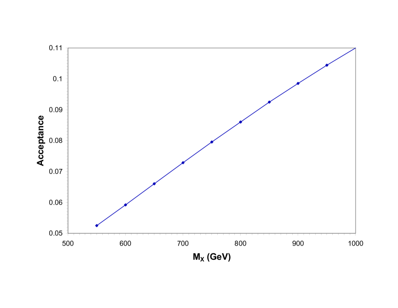
Figure 1: Plot of the kinematic and geometric acceptance rate, which is the fraction of $pp\rightarrow X\to ZZ\to 4l$ events that satisfy the imposed jet and leptonic cuts.

For this gold-plated signal, one can impose a further set of cuts [13] on the outgoing leptons:

• They reconstruct to two on-shell $Z$’s

• $|y(l)|<2.5$

• $p_{T}(l)>40\,{\rm GeV}$

• $p_{T}(Z)>{1\over 4}\sqrt{M^{2}(ZZ)-4M_{Z}^{2}}$

• $M(ZZ)>500\,{\rm GeV}$

In our analysis we integrate over the phase space of $pp\to X\to ZZ\to 4l$ events to determine the total kinematic and geometric acceptance rate of these cuts. This is defined to be the fraction of $pp\rightarrow X\to ZZ\to 4l$ events that satisfy the imposed jet and leptonic kinematic and geometric cuts. The results are plotted in fig. 1, which shows that about $5\%-10\%$ of the signal events passes these cuts in the interesting range of $X$ boson mass.

For the background, after imposing these cuts, one finds that in the mass range of interest ($M_{X}\sim 500-1000\,{\rm GeV}$), less than one background event survives in each $50\,{\rm GeV}$ bin with 100 $\,{\rm fb}^{-1}$ of integrated luminosity [13]. Detection of this process can therefore be achieved with 10 signal events in a $50\,{\rm GeV}$ bin centered on $M_{ZZ}$.

In fig. 2 we plot the total cross section $\sigma(pp\to X)$ at the LHC as a function of the $X$ boson mass, $M_{X}$. The various solid lines in the plot correspond to different choices of $\Lambda_{X}$. The dashed line in fig. 2 shows the required $pp\to X$ production cross-section in order to find a 10 event signal in a $50\,{\rm GeV}$ bin centered on $M_{ZZ}$ in $100\,{\rm fb}^{-1}$ in the $4l$ channel. For $M_{X}$ in the range $500-1000\,{\rm GeV}$, discovery can be made if $\Lambda_{X}\sim 100-150\,{\rm GeV}$.

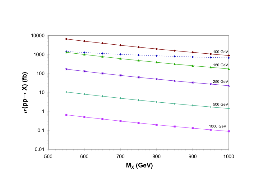
Figure 2: Plot of $\sigma(pp\rightarrow X)$ at $\sqrt{s_{pp}}=14\,{\rm TeV}$ LHC as a function of $M_{X}$ for various $\Lambda_{X}$. The dashed line corresponds to the cross-section required for detection at LHC in the $X\rightarrow ZZ\rightarrow 4l$ decay channel using the standard leptonic and jet cuts associated with this gold-plated vector boson fusion channel, discussed in text.

For any viable model, the fermion which run in the loop must be massive (to avoid the appearance of SM chiral exotics). This implies that $U(1)_{X}$ gauge symmetry must be broken [8]. The symmetry breaking effects may provide additional signals for the $U(1)_{X}$ gauge boson.

Conclusions

We have considered a physics scenario motivated by intersecting brane models, in which there are hidden $U(1)$ gauge groups under which the SM particles are uncharged. However, there can exist exotic matter, including non-vectorlike matter, that couples to both SM and hidden sector gauge groups. The resulting loop diagrams, along with tree-level higher-dimension couplings arising from the Green-Schwarz anomaly cancellation mechanism, generate an effective vertex that couples the hidden-sector gauge boson to two electroweak gauge bosons.

We defined $\Lambda_{X}$ as the mass-scale that suppresses these higher-dimensional couplings, and found that in the $X$ boson mass range of our study ($M_{X}\sim 500-1000\,{\rm TeV}$), LHC could detect this new physics through $pp\rightarrow X\rightarrow ZZ\rightarrow 4l$ processes provided $\Lambda_{X}\sim 100-150\,{\rm GeV}$. Although such a low $\Lambda_{X}$ is below the naive theory anticipations, it is important to remember that the contributions of vectorlike matter can be considerable, and the exponentially growing Hagedorn spectrum of states could put these values of $\Lambda_{X}$ within reach.

One should note that our estimates of detection likelihood are based only on the gold-plated decay channel $X\rightarrow ZZ\rightarrow 4l$. Although this mode combines a clean signal with a well-studied and highly suppressed background, it does suffer from small branching fractions. Other decay modes (for example, $ZZ\rightarrow ll+2j$, $WW\rightarrow 2l+2\nu$, or $\gamma Z$ decay) could collectively provide even better detection prospects.

For example, an especially interesting and unique signal in this context is the decay of $X\to\gamma Z\rightarrow\gamma ll$. ${\Gamma_{\gamma Z}\over\Gamma_{ZZ}}\sim 0.3$ implies a smaller rate of $\gamma Z$ intermediate states than $ZZ$, but the small branching fraction of $ZZ\rightarrow 4l$, along with the cleanness of a $\gamma$ signal make $X\rightarrow\gamma Z$ an important contributing mode for study. There has been some work on $\gamma ll$ signatures in the context of Higgs searches [15], but none apparently in conjunction with vector boson fusion production cuts. One would expect that appropriate cuts would also reduce the background for this signal to negligible levels, though a definitive statement would require a detailed background analysis which is beyond the scope of this letter. A comprehensive search strategy over all $X$ boson decay chains would be the ideal approach. This will be left for future work.

We conclude by noting that the couplings of the hidden sector $U(1)_{X}$ bosons to both SM fermions and SM gauge bosons depend on the details of the hidden sector. Although this fact makes it difficult to predict precisely how the exotic states will couple to SM states, the sensitivity gives one a chance to study and determine the dynamics of the hidden sector should these exotics appear at the LHC.

References

- [1] R. Blumenhagen, L. Goerlich, B. Kors and D. Lust, JHEP 0010, 006 (2000) [hep-th/0007024]; C. Angelantonj, I. Antoniadis, E. Dudas and A. Sagnotti, Phys. Lett. B 489, 223 (2000) [hep-th/0007090]; R. Blumenhagen, L. Goerlich, B. Kors and D. Lust, Fortsch. Phys. 49, 591 (2001) [hep-th/0010198]; G. Aldazabal, S. Franco, L. E. Ibanez, R. Rabadan and A. M. Uranga, J. Math. Phys. 42, 3103 (2001) [hep-th/0011073]; G. Aldazabal, S. Franco, L. E. Ibanez, R. Rabadan and A. M. Uranga, JHEP 0102, 047 (2001) [hep-ph/0011132]; M. Cvetic, G. Shiu and A. M. Uranga, Nucl. Phys. B 615, 3 (2001) [hep-th/0107166]; M. Cvetic, P. Langacker and G. Shiu, Nucl. Phys. B 642, 139 (2002) [hep-th/0206115];
- [2] R. Blumenhagen, V. Braun, B. Kors and D. Lust, hep-th/0210083; A. M. Uranga, Class. Quant. Grav. 20, S373 (2003) [hep-th/0301032]; M. Cvetic, P. Langacker, T. j. Li and T. Liu, Nucl. Phys. B 709, 241 (2005) [hep-th/0407178]; F. Marchesano and G. Shiu, Phys. Rev. D 71, 011701 (2005) [arXiv:hep-th/0408059]. M. Cvetic and T. Liu, Phys. Lett. B 610, 122 (2005) [hep-th/0409032]; F. Marchesano and G. Shiu, JHEP 0411, 041 (2004) [arXiv:hep-th/0409132]. C. Kokorelis, hep-th/0410134; J. Kumar and J. D. Wells, JHEP 0509, 067 (2005) [arXiv:hep-th/0506252]. C. M. Chen, T. Li and D. V. Nanopoulos, Nucl. Phys. B 732, 224 (2006) [hep-th/0509059]; B. Dutta and Y. Mimura, Phys. Lett. B 633, 761 (2006) [hep-ph/0512171]; M. R. Douglas and W. Taylor, JHEP 0701, 031 (2007) [hep-th/0606109].
- [3] K. R. Dienes, C. F. Kolda and J. March-Russell, Nucl. Phys. B 492, 104 (1997) [hep-ph/9610479]; J. Kumar and J. D. Wells, Phys. Rev. D 74, 115017 (2006) [hep-ph/0606183]; D. Feldman, Z. Liu and P. Nath, JHEP 0611, 007 (2006) [hep-ph/0606294]; W. F. Chang, J. N. Ng and J. M. S. Wu, Phys. Rev. D 74, 095005 (2006) [hep-ph/0608068], and hep-ph/0701254. D. Feldman, Z. Liu and P. Nath, Phys. Rev. D 75, 115001 (2007) [hep-ph/0702123]; W. F. Chang, J. N. Ng and J. M. S. Wu, 0706.2345 [hep-ph].
- [4] E. Kiritsis and P. Anastasopoulos, JHEP 0205, 054 (2002) [arXiv:hep-ph/0201295]. D. M. Ghilencea, L. E. Ibanez, N. Irges and F. Quevedo, JHEP 0208, 016 (2002) [arXiv:hep-ph/0205083]. C. Coriano, N. Irges and E. Kiritsis, Nucl. Phys. B 746, 77 (2006) [arXiv:hep-ph/0510332]. B. Dutta and J. Kumar, Phys. Lett. B 643, 284 (2006) [hep-th/0608188]. B. Dutta, J. Kumar and L. Leblond, hep-th/0703278.
- [5] P. Anastasopoulos, M. Bianchi, E. Dudas and E. Kiritsis, JHEP 0611, 057 (2006) [hep-th/0605225].
- [6] C. Coriano, N. Irges and S. Morelli, arXiv:hep-ph/0701010. C. Coriano, N. Irges and S. Morelli, arXiv:hep-ph/0703127.
- [7] D. Berenstein and S. Pinansky, Phys. Rev. D 75, 095009 (2007) [hep-th/0610104].
- [8] P. Anastasopoulos, T. P. T. Dijkstra, E. Kiritsis and A. N. Schellekens, Nucl. Phys. B 759, 83 (2006) [arXiv:hep-th/0605226].
- [9] G. L. Kane, W. W. Repko and W. B. Rolnick, Phys. Lett. B 148, 367 (1984); M. S. Chanowitz and M. K. Gaillard, Nucl. Phys. B 261, 379 (1985); S. Dawson, Nucl. Phys. B 249, 42 (1985); Z. Kunszt and D. E. Soper, Nucl. Phys. B 296, 253 (1988).
- [10] T. Han, G. Valencia and S. Willenbrock, Phys. Rev. Lett. 69, 3274 (1992) [hep-ph/9206246].
- [11] CTEQ Collaboration, CTEQ6 parton distribution functions, http://www.phys.psu.edu/cteq/.
- [12] R. N. Cahn et al., Phys. Rev. D 35, 1626 (1987); V. D. Barger, T. Han and R. J. N. Phillips, Phys. Rev. D 37 (1988) 2005; R. Kleiss and W. J. Stirling, Phys. Lett. B 200, 193 (1988); U. Baur and E. W. N. Glover, Phys. Lett. B 252, 683 (1990); V. D. Barger et al., Phys. Rev. D 44, 1426 (1991).
- [13] J. Bagger et al., Phys. Rev. D 52, 3878 (1995) [hep-ph/9504426].
- [14] D. L. Rainwater, M. Spira and D. Zeppenfeld, hep-ph/0203187. D. Green, hep-ex/0309031.
- [15] J. F. Gunion, G. L. Kane and J. Wudka, Nucl. Phys. B 299, 231 (1988).