Observational biases in Lagrangian reconstructions of cosmic velocity fields

Abstract

Lagrangian reconstruction of large-scale peculiar velocity fields can be strongly affected by observational biases. We develop a thorough analysis of these systematic effects by relying on specially selected mock catalogues. For the purpose of this paper, we use the Monge-Ampère-Kantorovitch (MAK) reconstruction method, although any other Lagrangian reconstruction method should be sensitive to the same problems. We extensively study the uncertainty in the mass-to-light assignment due to incompleteness (missing luminous mass tracers), and the poorly-determined relation between mass and luminosity. The impact of redshift distortion corrections is analyzed in the context of MAK and we check the importance of edge and finite-volume effects on the reconstructed velocities. Using three mock catalogues with different average densities, we also study the effect of cosmic variance. In particular, one of them presents the same global features as found in observational catalogues that extend to 80 $h^{-1}$Mpc scales. We give recipes, checked using the aforementioned mock catalogues, to handle these particular observational effects, after having introduced them into the mock catalogues so as to quantitatively mimic the most densely sampled currently available galaxy catalogue of the nearby universe. Once biases have been taken care of, the typical resulting error in reconstructed velocities is typically about a quarter of the overall velocity dispersion, and without significant bias. We finally model our reconstruction errors to propose an improved Bayesian approach to measure $\Omega_{\text{m}}$ in an unbiased way by comparing the reconstructed velocities to the measured ones in distance space, even though they may be plagued by large errors. We show that, in the context of observational data, it is possible to build a nearly unbiased estimator of $\Omega_{\text{m}}$ using MAK reconstruction.

Introduction

Galaxy redshift catalogues provide us with the radial velocities of the galaxies,

$$cz=H_{0}\,r+v_{r},$$ (1)

which are partly due to the global Hubble expansion ($H_{0}\,r$ with $H_{0}$ the present value of the Hubble parameter) and partly due to the line-of-sight components of the peculiar velocities ($v_{r}$). Peculiar velocities are the deviations of galaxy velocities from the uniform Hubble expansion, due to the non-homogeneous distribution of matter in the Universe. The peculiar velocities are thus tracers of mass distribution in the Universe and can have far-reaching implications for cosmology. As tracers of dark matter, peculiar velocities can be used to determine the local and global distribution of dark matter. From expression (1), it is evident that observations of galaxy redshifts ($z$) supplemented by measure of radial distances ($r$), would yield the peculiar velocities. However, measuring distances is a non-trivial exercise. The Tully-Fisher relation, surface brightness fluctuations, the Faber-Jackson relation for ellipticals (and their siblings, including the fundamental plane and the ${\rm D}_{\rm n}-\sigma$ methods, the Tip of the Red Giant Branch, Cepheids, and SNIa are the most usual methods for obtaining distances. The data gathered is however rather sparse: out of about a million galaxies whose redshifts are presently known with surveys such as 2dF and SDSS, the distances to only a few thousand have measured distances. Moreover, distances for most of these galaxies have too large peculiar velocity errors (due essentially to errors in distance measurements) to be useful in studying dynamics. For instance, distance indicators such as the Tully-Fisher relation suffer from 20% relative distance errors and thus produce quite noisy measurements at relatively moderate redshifts (i.e. $cz\ga 3000$ km s^-1). The data also suffers from selection biases (Strauss & Willick, 1995; Tully & Pierce, 2000). One way of reducing the error bars on distances is to average over many distance measurements for galaxies in clusters or groups and also by combining the results from different distance estimators. This treatment decreases the error bars on distances to about $8\%$ relative distance errors (Tully et al., 2007). Even though all these difficulties can be surmounted, one can finally hope to only have a sparse sample (as compared to redshift samples) of radial components of peculiar velocities. Fortunately, we now have Lagrangian velocity reconstruction schemes that are based solely on current redshift positions of mass tracers. The reconstructed velocities depend on cosmological parameters. Thus, comparing predictions obtained through Lagrangian reconstruction algorithms and the measured velocities may give estimations of these parameters.

This brings us to the main point that this paper tries to address: developing a robust and unbiased method of Lagrangian peculiar velocity reconstruction using redshift catalogues, in particular when observational effects distort most of the required data needed for the reconstruction of the dynamics. The reconstructed velocities are then compared to the measured ones using an ad hoc algorithm to yield a measurement of $\Omega_{\text{m}}$, the mean matter density of the Universe.

Throughout the paper, we will try to mimic observational effects as they appear in the most densely sampled currently available galaxy catalogue of the nearby universe which has been compiled by one of the authors (R. B. Tully). This galaxy catalogue is built from different sources such as ZCAT (Huchra et al., 1992) and SSRS (da Costa et al., 1988). Only galaxies for which $cz\leq 8000$ km s^-1 have been introduced in the catalogue. This catalogue is named NBG-8k, standing for NearBy Galaxy catalogue with a depth of 8000 km s^-1. Although selection criteria for this catalogue are not well defined, it will prove to be useful for the study of smaller galaxy catalogues such as NBG-3k (Tully et al., 2007).

For the purpose of this paper, we use a recently developed technique, called the Monge-Ampère-Kantorovitch reconstruction method (MAK hereafter), which is an approximation to the full non-linear dynamics to trace orbits back in time. This is a Lagrangian method, such as PIZA (Croft & Gaztanaga, 1997) or the Least-Action method (Peebles, 1989), and not a Eulerian technique such as, e.g., POTENT (Bertschinger & Dekel, 1989). One must note that the results of this paper are also valid for the other Lagrangian reconstruction methods as all the effects we are going to analyze are explainable in terms of gravitational dynamics. The MAK reconstruction has already been largely discussed when applied on numerical simulations (Mohayaee et al., 2006; Brenier et al., 2003). It is based on assuming that the dark matter displacement field is convex and potential, i.e. irrotational. In doing so, we exclude displacement fields which include multistreaming regions. The main result is that it is then possible to reconstruct accurately and uniquely the displacement field of dark matter particles between their original position and their current position. Practically, to solve the MAK problem, one must minimize a cost function for the assignment of a dark matter particle at the present comoving position ${\bf x}_{i}$ and its initial comoving position ${\bf q}_{j}$:

$$S_{\sigma}=\sum_{i=1}^{N}\left({\bf x}_{i}-{\bf q}_{\sigma(i)}\right)^{2}\;.$$ (2)

If the Universe is assumed to be initially homogeneous, which is a fair hypothesis supported by CMB data (e.g. WMAP first year in Bennett et al., 2003), then ${\bf q}_{j}$ must be distributed on a uniform grid and the solution to the MAK problem is unique and given by the assignment $\sigma$ which minimizes $S_{\sigma}$. The derived solution is then necessarily irrotational and derives from a convex potential. To solve this problem, we have implemented a parallel version of the so-called “auction” algorithm proposed by Bertsekas (1979). Of course, as we are using an approximation to the dynamics, the solution to the problem will be only valid above some scale (typically a few $h^{-1}$Mpc). Once the solution is found, the immediate output of MAK reconstruction is the nonlinear displacement field ${\bf\Psi}({\bf q})={\bf x}({\bf{q}})-{\bf q}$, which can be used to find the peculiar velocity field ${\bf v}$ using the first-order Zel’dovich approximation:

$${\bf v}_{i}=\beta{\bf\Psi}_{i}\;,$$ (3)

where the subscript $i$ indicates the comparison is achieved on the corresponding field averaged over the object $i$ (i.e. in a Lagrangian way), and the linear growth factor $\beta\simeq\Omega_{\text{m}}^{5/9}$ (Bouchet et al., 1995). This best fit for $\beta$ is valid as soon as $\Omega_{\text{m}}+\Omega_{\Lambda}=1$, $\Omega_{\Lambda}$ being the present dark energy density. It appears then that a direct comparison of ${\bf\Psi}_{i}$ against ${\bf v}_{i}$ should in principle give us $\beta$ and thus $\Omega_{\text{m}}$. Though naive measurements (Mohayaee & Tully, 2005) and preliminary studies (Branchini et al., 2002; Phelps et al., 2006) on mock redshift catalogues have already been tried, the observational biases and systematic errors in the velocity-velocity comparison have never been studied thoroughly.

This paper is organized as follows. In Section 1, we describe the simulation and the basic mock catalogues that are used in the rest of this paper. Subsequent mock catalogues integrate more and more observational features but are still based on the same original basic mock catalogues presented in this section. Section 2 gives a model for the error distribution on MAK velocities and discuss the first problematic features of the comparison between MAK and measured velocities. This error distribution helps us in particular to establish the likelihood analysis in Section 6. We go then to the first main topic of this paper in Section 3 by studying the systematic errors introduced by arbitrary mass-to-light assignments in redshift catalogues. This section includes a study of missing mass correction (§ 3.1), unknown $M/L$ function (§ 3.2) and incompleteness effects (§ 3.3; technical details are given in Appendix C). In Section 4, we discuss the problem of redshift distortions and the way to account for it during the MAK reconstruction. Section 5 is devoted to the handling of finite volume and edge effects, i.e. issues related to the zone of avoidance (§ 5.1), the choice of the Lagrangian volume of the reconstruction (§ 5.2), and finally the so-called cosmic variance (§ 5.3). The last section (§ 6) of this paper investigates the effect of distance measurement errors on the comparison between reconstructed and measured velocities, and proposes a maximum likelihood estimator (§ 6.2) to account for them in the measurement of $\Omega_{\text{m}}$. Results given by this estimator are then discussed in § 6.3.

1 Mock catalogues

To study various effects and systematic biases on the MAK reconstructed velocity field, we generated a number of mock catalogues extracted from a $N$-body simulation (§ 1.1). Although many recipes will be employed later to address various observational biases, we will always start from the same three “main” halo catalogues as described in § 1.2. The first catalogue aims to reproduce to some extent the main features of the local universe, in particular the presence of a large cluster at about 40 $h^{-1}$Mpc and a super-cluster at about 70 $h^{-1}$Mpc. The second and the third catalogues have less salient features but represent locally overdense and underdense realisations in order to address the problem of cosmic variance.

1.1 The $N$-body sample

Our $128^{3}$ particles $N$-body sample (Mohayaee et al., 2006) was generated with the public version of the $N$-body code HYDRA (Couchman et al., 1995) to simulate collisionless structure formation in a standard $\Lambda$CDM cosmology. The sample covers a comoving volume of 200³$h^{-3}$ Mpc³. The mean matter density is $\Omega_{\text{m}}=0.30$ and the cosmological constant $\Omega_{\Lambda}=0.70$. The Hubble constant is $H_{0}=65$ km s^-1 Mpc^-1. The normalisation of the density fluctuations in a sphere of radius 8 $h^{-1}$ Mpc, is $\sigma_{8}=0.99$. We note that this value of $\sigma_{8}$ is significantly larger than the value suggested by present WMAP data which sets $\sigma_{8}=0.74$ (Spergel et al., 2006), but this should not affect significantly the results presented in this paper. In fact, a lower $\sigma_{8}$ compared to $0.99$ would reduce both non-linearities and cosmic variance effects, hence improving the quality of the measurements.

As the velocity field presents significant fluctuations on a larger scale than for the density field, one may worry about the small size of the simulation volume. We have checked, using linear theory, that the velocity dispersion in $200^{3}h^{-3}$ Mpc³, for our cosmology, is $40$ km s^-1. This value has to be compared to the typical errors appearing while doing velocity reconstructions to ensure that cosmic variance effects are negligible for our purpose.

1.2 The basic mock catalogues

To build mock catalogues, we have selected haloes from the $N$-body experiment using a standard Friend-Of-Friend algorithm with a traditional value of the linking parameter given by $l=0.2$ (Efstathiou et al., 1988). Haloes with less than 5 particles, i.e. with mass smaller than $M_{\text{min}}=1.62\times 10^{12}\;h^{-1}\text{ M}_{\odot}$, were discarded. Fig. 1 shows the good agreement between the measured halo mass function and the Sheth & Tormen (2002) model for haloes with $M\ga M_{\text{min}}$. However about 63% of the mass is not clumped in these haloes and is distributed in the background field. In realistic galaxy samples such as the NBG-8k or the 2MASS catalogue the lower mass cut-off is of the order of $10^{11}\text{ M}_{\odot}$, a value much smaller than our $M_{\text{min}}$. To mimic galaxies with mass smaller than $M_{\text{min}}$, as will be required in the following, we just use dark matter particles unassigned to any halo as tracers. The catalogue containing all the haloes and all the field particles will be called FullMock. One could here worry that the $N$-body sample that we are using has a too low resolution as the spatial distribution of small halos is biased but not the particles of the background field. We have actually checked that using a $512^{3}$ $N$-body sample with nearly the same cosmology [the simulation is described in Colombi et al. (2007)] does not change any measurements presented in § 2.

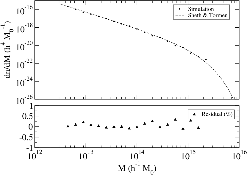
Figure 1: Sheth & Tormen mass function / Diffuse mass – The top panel of this plot gives the number density of haloes in a mass bin as a function of. the mass. The round points give the measurement of this function in the halo catalog whereas the dashed line is obtained using the Sheth & Tormen (2002) theory. The residuals between the prediction and the measurement are given in the lower panel (relative differences). Most of the time, the points are within a few percent of the theoretical prediction.

Out of FullMock, we have extracted three spherical cuts of radius 40 $h^{-1}$Mpc (hereafter denoted by 4k-mockX), where the velocity-velocity comparisons are conducted, and twice deeper counterparts (hereafter denoted by 8k-mockX) are used to give better constraints (§ 5.2) on the reconstruction within the volume of analyses. Each of these catalogues is centered in a different place in the simulation such that:

• 4k-mock6 is mildly overdense, with an effective mean matter density $\Omega_{\text{eff}}=0.35$, and contains 495 haloes. It is designed in such a way that large voids and large concentrations of matter (clusters or super-clusters) are present near its boundaries, similarly as found in real redshift catalogues of our local neighbourhood, such as the UZC (Falco et al., 1999), the NBG-3k (Shaya et al., 1995; Tully et al., 2007) and the NBG-8k. This catalogue and its deeper counterpart, 8k-mock6, are particularly suited to address edge effects on the NBG-3k (which terminates at Hydra and Centaurus clusters) and the NBG-8k (which stops at the Great Wall), respectively.

• 4k-mock7 is highly overdense,with $\Omega_{\text{eff}}=0.50$, and contains 656 haloes. Very little mass has come in and out of this volume: it behaves somewhat like an isolated universe, with small external tides.

• 4k-mock12 is underdense, with $\Omega_{\text{eff}}=0.19$, and contains 213 haloes. It presents as well a low level of density fluctuations along its boundary.

While there is no ambiguity in setting up a $128^{3}$ MAK mesh when using all the haloes and the background particles (such as in FullMock), it is less trivial to consider lower resolution meshes that will be used in some of the subsequent analyses. Indeed, the number of mesh elements assigned to each tracer is not necessarily an integer anymore. Appendix A details the general procedure used to associate elements of the MAK mesh to each tracer.

2 Errors in MAK velocities

Before going over observational issues, we address errors intrinsic to MAK reconstruction. First, there is scatter in the reconstruction of the displacement field itself which is expected to be rather small (Mohayaee et al., 2006). Second, there is scatter due to the Zel’dovich approximation one uses to convert a displacement field into a velocity field and to deal with redshift distortions. An accurate knowledge of the distribution of errors on the reconstructed velocities is eventually required for the likelihood analysis we want to introduce in § 6.2. In this section, we measure such a distribution in real space while redshift space will be addressed in § 4. In principle, the width of such a distribution is expected to increase when observational biases are taken into account while its shape should not change significantly.

We consider, in this section, reconstructions based on the catalog FullMock, for which periodic boundary conditions are applied to avoid edge effect problems. We also assume that we know the mass of all of described catalog objects (haloes and individual particles). Our subsequent reconstructions have a resolution within $64^{3}$ and $128^{3}$ mesh elements. We will thus present two reconstructions obtained on two different initial MAK mesh, $128^{3}$ and $64^{3}$, obtained using the procedure presented in Appendix A. The results on the reconstructed displacement field are given in Fig. 3. These plots give the distribution of differences, $P_{\text{DE}}$, between the line of sight component of the reconstructed displacement field and the “exact” one, given by the simulation.

The dot-dashed and dashed curves correspond to a least-square fit of the function $P_{\text{DE}}$ corresponding to the $128^{3}$ reconstruction respectively with a Gaussian fit, and a Lorentzian fit given by

$$P_{\text{Lor}}(x)=\frac{1}{\pi B}\frac{1}{1+\frac{x^{2}}{B^{2}}}\text{ .}$$ (4)

Examination of Fig. 3 supports the Lorentzian approximation with $B=35$ km s^-1, which reproduces better the long tails of $P_{\text{DE}}$ than the Gaussian.

The width, $B$, of $P_{\text{DE}}$ is rather small compared to the line-of-sight dispersion, $\langle\beta^{2}\Psi_{r}^{2}\rangle^{1/2}\simeq 292$ km s^-1, as expected. Naturally, the function $P_{\text{DE}}$ is slightly flatter and larger for the $64^{3}$ case than for the $128^{3}$ one. However, the far end tails of $P_{\text{DE}}$ are the same for $64^{3}$ and $128^{3}$. In this regime, the measurements are not influenced by the resolution of the grid used to perform the reconstruction but rather by the inability of MAK to reproduce the internal dynamics of massive, relaxed objects (Mohayaee et al., 2006).

Reconstruction $128^{3}$	Reconstruction $64^{3}$	Simulation

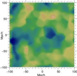
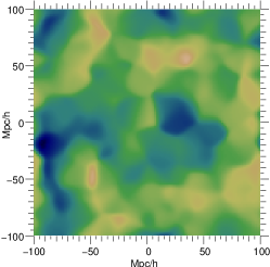
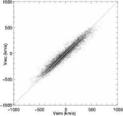
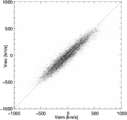
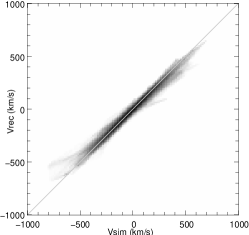
Figure 2: Velocity field reconstruction on FullMock – Top panels: A slice of the line-of-sight component of the simulated velocity field, $v_{\text{r,sim}}$, and the reconstructed one, $v_{\text{r,rec}}$, after smoothing with a 5 $h^{-1}$Mpc Gaussian window. The observer is at the center of this slice. Bottom panels: Scatter plots between $v_{\text{r,sim}}$ and $v_{\text{r,rec}}$ for invidual haloes (left) and after smoothing (right).

Fig. 4 is similar to Fig. 3 but considers line of sight reconstructed velocities vs “exact” ones. Although Zel’dovich approximation introduces extra noise as shown by a wider width of the distribution, $P_{DE}$ remains roughly Lorentzian with a small width $B=48$ km s^-1. This error variance is grossly 25% higher than the expected velocity field variance on the simulation volume (§ 1.1). We are thus not affected by cosmic variance effects that could have been induced by modes larger than the box size of the simulation.

These results are fully supported by the examination of Fig. 2. However, the lower panels of this figure shows that the joint distribution $P(v_{\text{sim}},v_{\text{rec}})$ presents non-trivial tails above the diagonal line in the lower left quadrant and below the diagonal line in the upper right quadrant, respectively. These tails do not disappear even after smoothing of the velocity field with a 5 $h^{-1}$Mpc Gaussian window. This is due to non-linear features in the dynamics not taken into account by our MAK+Zel’dovich prescription, which produces a slightly smoother velocity field than the real one. As a result, upper left panel of Fig. 2, which corresponds to the reconstruction, is less contrasted than the upper right one, which corresponds to the simulation.

These non-linear tails give a propeller shape to $P(v_{\text{sim}},v_{\text{rec}})$ which is susceptible to inducing a small bias on the final velocity-velocity comparison. For instance, one can estimate the slope of the lower left scatter plot of Fig. 2 using the ratio $s=\sigma_{v,rec}/\sigma_{v,sim}$, where $\sigma^{2}_{v,rec}$ and $\sigma^{2}_{v,sim}$ are the variances of the reconstructed and simulated velocity fields, respectively. In this case, the estimated $\beta$ is biased to higher values by about 7%. However, visually inspecting the scatter shows no measurement bias should occur if only the central part of the scatter is used for the computation. To achieve this, we have first applied an adaptive SPH filter on the scatter plot to produce a Probability Density Function (PDF), which is probed by the scatter in the points, on a regular mesh grid. We then compute the 1.5$\sigma$ isocontour which encloses the region where the integrated PDF is equal to 68%. This procedure has already been used in Colombi et al. (2007) for the gravity-velocity comparison with total success. Only the points enclosed by the 1.5$\sigma$ isocontour are used to compute the new $s_{med,68}$ coefficient. The $\beta$ parameter deduced from $s_{\text{med},68}$ is now statistically unbiased. Similarly, we define two other slope estimators $s_{\text{min},68}$ and $s_{\text{max},68}$ whose relevance is discussed in Appendix B. In this paper, until § 6, we will only discuss the measurement of $\Omega_{\text{m}}$ obtained through the estimation of $s_{\text{med},68}$. The $\Omega_{\text{m}}$ obtained by this method is identified by a “$1.5\sigma$” to make a difference with the one obtained through the likelihood analysis that will be established in § 6 and which is identified by a “$\mathfrak{L}$” in the tables and figures. A test of this method on a simulated scatter distribution, whose shape is built on analysis of reconstruction errors, is detailed in Appendix D.

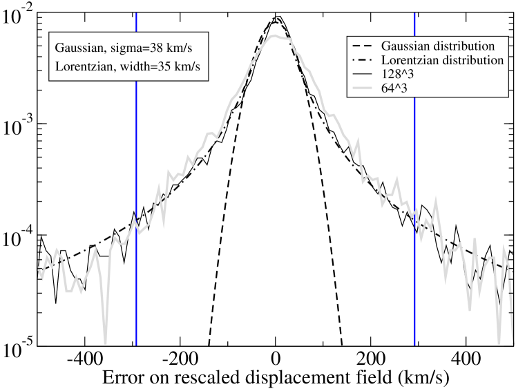
Figure 3: Error in reconstructed displacements – This plot displays the probability distribution of the quantity $\beta\left(\Psi_{\text{r,rec}}-\Psi_{\text{r,sim}}\right)$ measured in FullMock (solid curve), where $\Psi_{\text{r,rec}}$ and $\Psi_{\text{r,sim}}$ are the line-of-sight component of the reconstructed and simulated displacement fields, respectively, after choosing an observer at the center of the simulation box. The dashed and dot-dashed curves give the best fit of a Gaussian and a Lorentzian distribution, respectively.

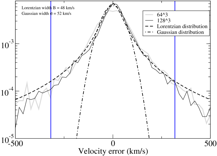
Figure 4: Error in reconstructed velocities – Same as in Fig. 3 but the solid curve corresponds to the probability distribution of the quantity $v_{\text{r,rec}}-v_{\text{r,sim}}$, where $v_{\text{r,rec}}$ and $v_{\text{r,sim}}$ are the line-of-sight reconstructed and simulated velocities, respectively.

3 Mass-to-light assignment

Most reconstruction methods, including ours, infer the total matter distribution as a function of the visible matter distribution traced by galaxies. The fundamental assumption one usually makes is that the relation between these two distributions is highly deterministic. In other words, one assigns to each galaxy of a given luminosity $L$ a dark matter concentration (a halo) of mass $M=f(L)$. However, there are several issues in this procedure:

• Mass-to-light ratio – The choice of a function $f(L)$ influences considerably the results and is expected to introduce significant bias on the measured $\beta$ if performed unwisely. Now, the function $f(L)$ is coarsely determined (Tully, 2005; Marinoni & Hudson, 2002) from direct measurements in observations. One way to infer this function is to rely on semi-analytic models of galaxy formation, but this represents a very strong prior on the measurements. Furthermore, $f(L)$ remains a mean relation around which there can be some significant scatter. This dispersion can as well introduce some significant biases.

• Missing tracers / Magnitude limitation – Even if function $f(L)$ is perfectly known, fainter galaxies are still missing in the catalogues due to the limitations of observational instruments. For instance, in magnitude-limited catalogues, the number density of detected galaxies decreases with distance from the observer. These missing tracers have unknown positions and correspond to a part of the dark matter distribution which is totally undefined. This missing mass has to be taken into account in some way.

In what follows, we will first address the second issue in a very simple way which assumes that the function $f(L)$ is well known (namely the masses of dark matter haloes themselves) but there is a fixed low-mass cut-off. The problem then consists in determining the unknown part of the dark matter distribution (namely the particles unassigned to any halo). Clearly it is correlated with the detected mass tracers but less clustered. There are two extreme ways to locate this missing mass

1. associate it with the existing tracers as usually done with the analysis of real observations

2. associate it with a uniform background.

Of course, the real solution is somewhat intermediate between (a) and (b) as will be shown in § 3.1.

Then, we turn in § 3.2 to the issue of the choice of $f(L)$. In this paper, we prefer to be as free as possible from strong priors so we deliberately do not use results from semi-analytic models of galaxy formation. Instead, we use determinations of $f(L)$ from observational data but, unfortunately, there are large uncertainties in these measurements. The point here is to quantify, quite heuristically though, the effect of these uncertainties, random or systematic, on the measurement of $\beta$. Indeed, one is both confronted with a possibility of a wrong approximation of $f(L)$ and most probably a large scatter around this mean relation.

In sufficiently deep galaxy catalogues, the effect of the missing tracers is expected to be negligible close to the observer and, in general, to increase with the distance from the observer. With appropriate weighting of the data, one can minimize the bias brought by the procedure used to infer the missing mass distribution far from the observer. In § 3.3, we shall illustrate this point by considering the case of a magnitude-limited catalogue where all the missing mass is associated with the existing tracers [method (a) above].

3.1 Missing tracers

	Simulation
All missing mass in haloes	Optimal compromise	All missing mass to background

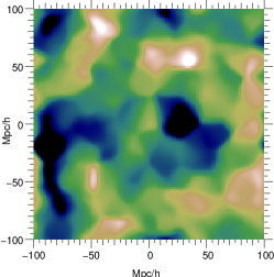
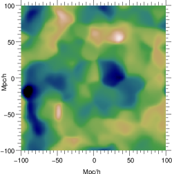
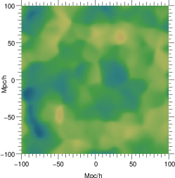
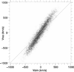
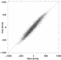
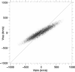
Figure 5: Diffuse mass correction – The top panel gives a slice of the line-of-sight component of the simulated velocity field, after smoothing with a 5 $h^{-1}$Mpc Gaussian window. The observer has been put at the center of this slice. The second row of panels represents the line-of-sight component of the reconstructed velocity field, smoothed in the same way, for different corrections of the diffuse mass. The third row of panels give the scatter distribution of individual reconstructed velocities of haloes vs simulated ones. The left panels give the result of a reconstruction on a mock catalog which only contain the haloes and not the background field but at the same time conserves the total mass of the catalog by reassigning the missing mass to the haloes. The right panels give the result for a reconstruction based on a mock catalogue for which the missing diffuse mass is represented by a background field composed of particles placed randomly in the catalogue. The center panels give the result of a reconstruction on a mock catalogue which only contain the haloes and a random background field. The mass that have been initially removed from the mock catalogue (the background “galaxies”) is reassigned as follows: 60% to haloes and 40% to the background.

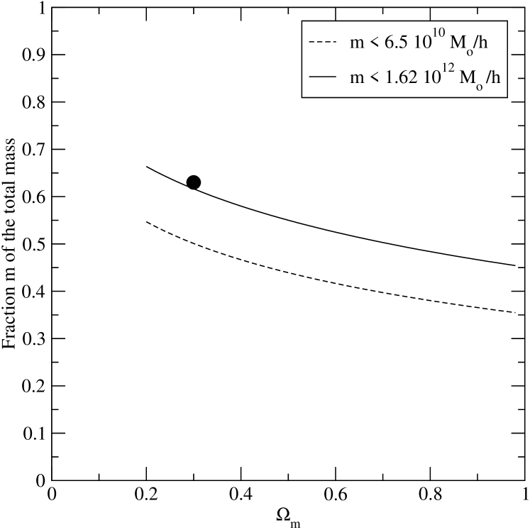
Figure 6: Diffuse mass – In this plot, we represent the fraction of the clustered mass below two mass resolutions for a standard $\Lambda$CDM type cosmology ($h=0.65$, $\sigma_{8}=0.99$). We used a power spectrum as proposed by Bardeen et al. (1986). The curvature of the Universe is kept flat while $\Omega_{\text{m}}$ varies. This fraction is plotted for mass resolutions: $2.5\times 10^{12}\text{ M}_{\odot}$ (corresponding to the lower mass limit of haloes in our simulation) and $10^{11}\text{ M}_{\odot}$ ($\simeq 10^{9}\text{ L}_{\odot,B}$). The unclustered fraction in FullMock is given by the back filled circle. The fraction of mass below both of these limits is still considerable.

Fig. 6 shows the expected fraction of the total mass below a fixed threshold as a function of $\Omega_{\text{m}}$, using the Sheth & Tormen (2002) model (see also Fig. 1). The solid line corresponds to the mass cut-off of haloes in FullMock and agrees, as expected, with the measurement in the simulation for $\Omega_{\text{m}}=0.30$. Here, 63% of the mass is outside of the haloes, which represent our “galaxies” with known $M/L$ ratio. The particles not linked to the haloes represent the missing mass. In Fig. 2, their exact location was used to perform the reconstruction. The only information available now is the distribution of “visible galaxies”. The missing mass needs to be redistributed using only these pieces of information. We propose two extreme ways to do so:

1. All missing mass to background – Prior to the reconstruction, the missing mass is divided into particles which are randomly put in the catalog following a poissonian distribution. In the example illustrated by the right panels of Fig. 5 we choose for simplicity particles of the same mass as those in the simulation.

2. All missing mass in haloes – The missing mass is attributed to the existing haloes in proportion to their masses, as illustrated by left panels of Fig. 5. This approach is equivalent, in real observations, to multiplying the $M/L$ ratio of galaxies or group of galaxies by a constant $\alpha>1$.

Obviously, in I, the screening effect due to the background is exagerated, hence the reconstructed velocity is less contrasted and $\beta$ is over-estimated to compensate for this. In II, on the other hand, the potential wells are more contrasted than they should be, which leads to the opposite effect. At this point, it is extremely tempting to try to find a simple compromise between I and II as illustrated by middle panels of Fig. 5 where 60% of the missing mass was linked to the tracers and the remaining to a uniform background. With this particular choice of the redistribution, the match between the reconstructed and the simulated velocity fields is spectacular. This result is non-trivial given the simplicity of the handling of this sixty three percent missing mass all the more since the scatter on the middle-lower panel of Fig. 5 is of the same order of that of the lower left panel of Fig. 2, where all the tracers contribute optimally.

Although the choice of the optimal redistribution remains a priori unknown in a real galaxy catalogue one can at least infer error bars from I and II. In that framework, Fig. 5 unfortunately provides quite a bad constraint on $\beta$, $0.36\la\beta\la 0.85$. However, in real galaxy catalogues, such as the NBG-3k or the NBG-8k, the minimum luminosity is of the order of $10^{9}$ L_⊙. This corresponds to a less abrupt mass cut-off, $M_{\text{cut}}\sim 10^{11}\text{ M}_{\odot}$, than in Fig. 5, where $M_{\text{cut}}=2.5\times 10^{12}\text{ M}_{\odot}$. Therefore, one expects the problem of missing mass to be less saliant in real observations, as illustrated by the dashed curve of Fig. 6. Furthermore, an appropriate use of mock catalogues can help at calibrating the redistribution of mass, as performed in middle panels of Fig. 5.

3.2 Mass-to-light ratio

$$\begin{array}[]{c}\text{\begin{minipage}{35.56593pt}\centering Halo catalog\@add@centering\end{minipage}}\xrightarrow{\text{\begin{minipage}{28.45274pt} \begin{center} Tully \end{center} \end{minipage} }}\text{\begin{minipage}{44.10185pt}\centering Luminosity Catalog\@add@centering\end{minipage}}\xrightarrow{\text{\begin{minipage}{28.45274pt} \begin{center} $\frac{M}{L}=a$ \end{center} \end{minipage} }}\text{\begin{minipage}[t]{28.45274pt}\centering MAK\@add@centering\end{minipage}(T-C)}\\ \\ \text{\begin{minipage}{35.56593pt}\centering Halo catalog\@add@centering\end{minipage}}\xrightarrow{\text{\begin{minipage}{28.45274pt} \begin{center} Tully \end{center} \end{minipage} }}\text{\begin{minipage}{44.10185pt}\centering Luminosity Catalog\@add@centering\end{minipage}}\xrightarrow{\text{\begin{minipage}{28.45274pt} \begin{center} MH \end{center} \end{minipage} }}\text{\begin{minipage}[t]{28.45274pt}\centering MAK\@add@centering\end{minipage}(T-MH)}\\ \\ \text{\begin{minipage}{35.56593pt}\centering Halo catalog\@add@centering\end{minipage}}\xrightarrow{\text{\begin{minipage}{28.45274pt} \begin{center} Tully + scatter \end{center} \end{minipage} }}\text{\begin{minipage}{44.10185pt}\centering Luminosity Catalog\@add@centering\end{minipage}}\xrightarrow{\text{\begin{minipage}{28.45274pt} \begin{center} Tully \end{center} \end{minipage} }}\text{\begin{minipage}[t]{28.45274pt}\centering MAK\@add@centering\end{minipage}(TS-T)}\end{array}$$

Figure 7: $M/L$ assignment – Sketch of the procedures used to test the influence of a choice of a $M/L$ assignment, as explained in the main text.

To test how the choice of mass assignment to galaxies or group of galaxies affects the results we consider the three following cases, as summarized in Fig. 7:

1. T-C case: a galaxy catalogue is extracted from FullMock by associating a luminosity $L(M)$ to each dark matter halo or background particle using Tully’s latest best fit of the group mass-luminosity relation (Tully, 2005, see Fig. 8)

   $$\frac{L_{B}}{L_{\odot}}=2700\left(\frac{M}{M_{\odot}}\right)^{0.59}\mathrm{e}^{-6\times 10^{11}M_{\odot}/M},$$ (5)

   which gives the luminosity in the B band for groups in the mass range $10^{11}\,\,\text{M}_{\odot}\text{ - }10^{15}\,\,\text{M}_{\odot}$. Then a new mass is given to each tracer assuming

   $$M/L=\text{constant,}$$ (6)

   as often used in the litterature, and MAK reconstruction is performed on a resampling of this mass distribution.

2. T-MH case: a less extreme case than assuming $M/L=$ constant consists in separating the tracers in three broad classes: faint galaxies, luminous galaxies and group/clusters of galaxies, as performed by Marinoni & Hudson (2002), hereafter MH. To do this, they used a simple mapping between the Schechter luminosity function and the Press-Schechter mass function that reads as follows

   $$\begin{array}[]{lr}M/L=1.15\;10^{7}\left(\frac{L}{L_{\odot}}\right)^{-0.5}h\frac{M_{\odot}}{L_{\odot}}&\frac{L}{L_{\odot}}<4\;10^{10}\\ M/L=128h\frac{M_{\odot}}{L_{\odot}}&4\;10^{10}<\frac{L}{L_{\odot}}<4\;10^{11}\\ M/L=3.6\;10^{-4}\left(\frac{L}{L_{\odot}}\right)^{0.5}h\frac{M_{\odot}}{L_{\odot}}&\frac{L}{L_{\odot}}>4\;10^{11}\end{array}$$ (7)

   as shown in upper panel of Fig. 8. In this framework, we generated the same catalog as in T-C case but it was analyzed assuming the $M/L$ function given by Eq. (7).

3. TS-T case: assuming that we have an unbiased estimator of the $M/L$ function, there can still be a scatter around this mean value that can increase the errors and also introduce systematic bias. We test this by multiplying the mass of each halo of FullMock by a random number $x$ such that $\log_{10}x$ is uniformly distributed in $[-1,1]$, prior to MAK reconstruction, which is performed on a resampling of the halo catalog following the procedure explained in Appendix A. Note that the mass of background particles remains unchanged during the process, which corresponds to 63% of the matter distribution being unaffected by the scattering. However, applying the scatter to small mass haloes only introduces a local additional noise which should not have any significant consequences on the reconstruction accuracy for which deeper potential wells are in fact more critical.

We want to highlight the fact that each of these transformations, actually corresponding to transforming the mass of an object of FullMock through a $M\rightarrow L\rightarrow M$ operation, does not correspond to an identity. One actually gets a new set of masses attached to each tracer which is different from the original one. Moreover, the output mass distribution $P_{\text{mass,out}}(M)$ may be fundamentally different from the input one $P_{\text{mass,in}}(M)$. Indeed, computing $P_{\text{mass,out}}(M)$ is equivalent to performing a weighted average of $P_{\text{mass,in}}(M)$. This procedure induces a global reshaping of the distribution. Consequently, the statistical properties of the corresponding mass density field may be affected.

More technically, during the procedure used to construct all the catalogues above, total mass conservation is enforced. Note that the total mass depends on $\Omega_{\text{m}}h^{2}$, but this normalization does not affect MAK displacements, which are sensitive to density contrasts only. Parameters $\Omega_{\text{m}}$ and $h$ in fact intervene while performing velocity-velocity comparison and while converting distances to velocities (§ 6), respectively.

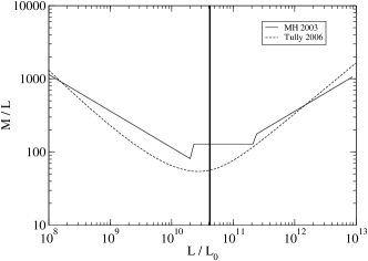
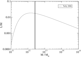
Figure 8: M/L function – The above two plots give the forward and inverse mass-to-light functions for both Tully (2005) and Marinoni & Hudson (2002) fits. The top panel gives the $M/L$ as a function of the luminosity $L$, the bottom panel gives $L/M$ as a function of the mass $M$.

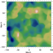
(TS-T)	(T-C)	(T-MH)

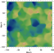
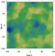
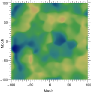
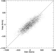
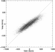
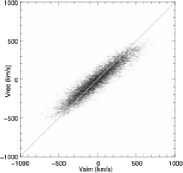
Figure 9: $M/L$ bias – The top panel gives the expected line-of-sight component $v_{r}$ of the velocity field, smoothed with a 5 $h^{-1}$Mpc Gaussian filter, as given by the simulation in a thin slice of the simulation containing the observer. The middle panels gives the reconstructed $v_{r}$ field, with the same smoothing, after having applied each of the transformations specified in Fig. 7 to FullMock. The lower panels gives the scatter between the reconstructed and simulated peculiar velocities for each of the transformations.

Table 1: $M/L$ bias effect – This table gives the results obtained using different statistical tools. We also measured $\Omega_{\text{m}}$ using six different methods: the label $s$ means we used the slope estimated by using all objects, the label $\mathfrak{L}$ is used when $\Omega_{\text{m}}$ has been determined using the likelihood analysis, and the label 1.5$\sigma$ is used when the slope is estimated using only the objects within the 1.5$\sigma$ isocontour of the PDF between reconstructed velocities and simulated velocities (method described in § 2).

Transf.	Velocity			$\Omega_{\text{m}}$ ($s$)	$\Omega_{M}$ ($\mathfrak{L}_{\text{min}}$)	$\Omega_{M}$ ($\mathfrak{L}_{\text{max}}$)	$\Omega_{M}$ (1.5$\sigma$,$s_{\text{med}}$)	$\Omega_{M}$ (1.5$\sigma$,$s_{\text{min}}$)	$\Omega_{M}$ (1.5$\sigma$,$s_{\text{max}}$)
	$s$	$r$	$\sigma$
None	0.88	0.89	0.58	0.38	0.30	0.31	0.30	0.28	0.31
TS-T	0.90	0.78	0.64	0.36	0.26	0.30	0.28	0.24	0.33
T-MH	0.80	0.80	0.60	0.45	0.33	0.38	0.36	0.32	0.40
T-C	0.71	0.78	0.63	0.55	0.40	0.48	0.44	0.37	0.51

As expected, random uncertainty on the mass determination does not introduce any bias, it only increases the scatter in the measurements as illustrated by the lower left panel of Fig. 9. A more important issue is the global knowledge of the $M/L$ relation. Indeed, it seems that the slope of this relation influences greatly the results, as illustrated by the middle and right panels of Fig. 9. Clearly, if the galaxies follow the Tully formula (5), it is definitely wrong to assume constant $M/L$ and even the MH fit introduces a significant bias, although it is well within the observational errors compared to Eq. (5). It must be noted that this bias can be turned into an advantage if one does not want to measure $\Omega_{\text{m}}$ but the $M/L$ relation. Indeed, WMAP experiment (Bennett et al., 2003; Spergel et al., 2006) coupled with an analysis of the power spectrum of large scale density of galaxies (Tegmark et al., 2006) gives good constraints on the real $\Omega_{\text{m}}$ now. Our method, on the other hand, is able to measure the discrepancy between the measured $\beta$ and the expected growth factor $\beta_{\text{expected}}=\Omega_{\text{m}}^{5/9}$ (i.e. the bias). This measurement may give an idea of how wrong is the assumed $M/L$ relation prior to the reconstruction and may push us to try different plausible $M/L$ functions. Thus our method is able to measure the way that the matter is distributed in the Universe once it is given its average density $\Omega_{\text{m}}$. On the other hand, if the above bias is well understood, this method helps at reducing the degeneracy in the determination of cosmological parameters. Indeed, our posterior probability on $(\Omega_{\text{m}},h)$ gives a constraint orthogonal (for example see the results in Mohayaee & Tully, 2005) to the one obtained from the WMAP experiment and from the galaxy statistics of the SDSS.

3.3 Magnitude limitation

Magnitude-limited sampling of mass tracers introduces a new type of problem: flux limitation decreases the mass resolution toward the outer edges of the catalogue contrary to the homogeneous case studied in § 3.1. Usually, the incompleteness is handled by boosting uniformly the luminosities of galaxies at a given distance from the observer (Branchini et al., 2002), prior to conversion of luminosities into masses. This is a fair approach if $M/L=\text{constant}$, modulo the issues discussed in § 3.1. However, this method is in general questionable for non-trivial $M/L$ relations as in Eq. (5) or if different $M/L$’s are assigned to galaxies with different types. In these last two cases, the missing mass correction should be applied to the mass distribution itself instead of the luminosity one, to avoid systematic errors on mass assignments, hence on reconstructed velocities. This unfortunately requires a prior assumption on the value of $\Omega_{\text{m}}$, but only slightly complicates the analyses.

In the observational data, galaxies are separated into two populations: groups of galaxies (Tully, 1987) and field galaxies. These two populations should be treated separately, keeping in mind that the groups are the most critical because their gravitational influence is much larger than individual field galaxies and they have better peculiar velocity measurements.

The full procedure consisting of creating a magnitude-limited mock catalogue and recovering the mass distribution is detailed in Appendix C. Let us recall that, in our mock catalogues, groups of galaxies are simulated dark matter haloes with more than 5 particles while background galaxies are identified with dark matter particles unassigned to any halo. We list here the key steps we used to correct for incompleteness:

1. The total apparent luminosities of groups of galaxies is obtained assuming a global or a local Schechter luminosity distribution for the considered groups. The intrinsic luminosity is computed trivially from the total apparent luminosity and the redshift of the group.

2. The intrinsic luminosity of the remaining unbound galaxies (thus field galaxies) is also determined, straightforwardly.

3. Then, masses are estimated by assigning appropriate $M/L$ to each object of I and II.

4. The local missing mass from undetected background galaxies is inferred from the detected mass distribution. This requires a prior on $\Omega_{\text{m}}$.

5. This missing mass may either be reassigned locally to detected field galaxies of II (our choice) or be introduced by the mean of new randomly positioned tracers, as discussed in § 3.1.

To examine the effects of systematics in the correction for incompleteness, we use 8k-mock6 and choose a flux limit such that the resulting mock catalogue has an incompleteness similar to NBG-8k, as shown in Fig. 10. Results are summarized in Fig. 11 and in Table 2.

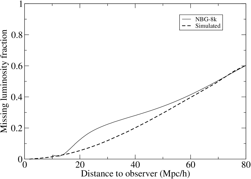
Figure 10: Magnitude limitation – Solid line: NBG-8k predicted luminosity incompleteness at the given distance from the observer. Dashed line: Simulated luminosity incompleteness in 8k-mock6. The incompleteness is expressed in terms of missing luminosity fraction at the specified distance.

The reconstructed radial peculiar velocities $v_{\text{r,rec}}$ are behaving extremely well. On average, the comparison between simulated and reconstructed velocity fields is surprisingly good in a volume of radius 80 $h^{-1}$Mpc, even though the edge misses locally 98% of the field galaxies which represents 60% of the total mass in our mock catalogue. It means that, though we keep only 2% of the field galaxies, they suffice, in addition to the groups, for a reasonably fair recovery of the large-scale peculiar velocity field. Note the small bias in the scatter of the lower right panel of Fig. 11, resulting in a slightly larger $\Omega_{\text{m}}=0.38$ than the expected value of 0.30, but in good agreement with the effective value of 0.35 expected in the corresponding volume (see § 5.3 on cosmic variance effects). This bias might be the consequence of our treatment of the missing mass coming from undetected tracers as discussed, in detail in Appendix C (point B).

Simulated	Reconstructed
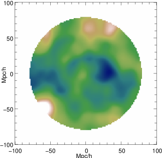
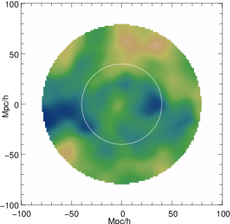
Comparison in 80 $h^{-1}$Mpc	Comparison in 40 $h^{-1}$Mpc

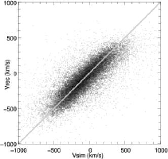
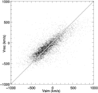
Figure 11: Incompleteness: magnitude limitation – Top panels: A slice of the line-of-sight component of the simulated velocity field in 8k-mock6 and the reconstructed one, after smoothing with a 5 $h^{-1}$Mpc Gaussian window. The displayed slice is chosen to include the observer in $(0,0)$. The white circle in the right panel gives the size of the 40 $h^{-1}$Mpc sphere embedded in the 80 $h^{-1}$Mpc one. Bottom panels: The scatter plots compare the reconstructed and simulated velocities of objects in the 80 $h^{-1}$Mpc region (left panel) and in the 40 $h^{-1}$Mpc volume (right panel).

Table 2: Incompleteness: magnitude limitation – Column description is given in the caption of Table 1.

Volume	Velocity field			$\Omega_{\text{m}}$ ($s$)	$\Omega_{\text{m}}$ ($\mathfrak{L}_{\text{min}}$)	$\Omega_{\text{m}}$ ($\mathfrak{L}_{\text{max}}$)	$\Omega_{\text{m}}$ (1.5$\sigma$,$s_{\text{med}}$)	$\Omega_{\text{m}}$ (1.5$\sigma$,$s_{\text{min}}$)	$\Omega_{\text{m}}$ (1.5$\sigma$,$s_{\text{max}}$)
	$s$	$r$	$\sigma$
8k	0.86	0.77	0.64	0.39	0.26	0.31	0.29	0.25	0.34
4k	0.77	0.75	0.66	0.48	0.37	0.45	0.38	0.30	0.47

4 Redshift distortion

The input of MAK reconstruction is the position of objects in real space as needed by Eq. (2). However redshift catalogues give us galaxy positions in redshift space, namely $s_{r}=Hd+v_{r}$, where $s_{r}$ is the redshift distance, $d$ is the luminosity distance between the observer and the object and $v_{r}$ is the line-of-sight peculiar velocity. To account for redshift distortions, we must correct for two major effects:

• “Fingers-of-god” correspond to an elongation of dense structures along the line of sight, such as clusters of galaxies, due to random motions of galaxies within these structures.

• Kaiser effect (Kaiser, 1987) is a large-scale effect coming from the coherent part of the cosmic flows, which, for instance, increase the overall density contrast.

Table 3: Redshift reconstruction – Column description is given in the caption of Table 1.

$s$	$r$	$\sigma$	$\Omega_{\text{m}}$ ($s$)	$\Omega_{\text{m}}$ ($\mathfrak{L}_{\text{min}}$)	$\Omega_{\text{m}}$ ($\mathfrak{L}_{\text{max}}$)	$\Omega_{\text{m}}$ (1.5$\sigma$,$s_{\text{med}}$)	$\Omega_{\text{m}}$ (1.5$\sigma$,$s_{\text{min}}$)	$\Omega_{\text{m}}$ (1.5$\sigma$,$s_{\text{max}}$)
0.83	0.46	0.95	0.50	0.22	0.29	0.27	0.22	0.33

Fingers-of-god effects can be easily removed by simply collapsing groups or clusters to a single point, as usually performed in the literature. However, such a procedure is generally carried out in a rather ad-hoc way and is certainly not free of biases.

The Kaiser effect can be accounted for by modifying the cost function (2) using the Zel’dovich approximation to infer line-of-sight peculiar velocities as functions of the sought displacement field (Mohayaee & Tully, 2005; Valentine et al., 2000). If ${\bf s}({\bf q})$ is the redshift coordinate of a particle originally at ${\bf q}$ then the total cost (2) of the association $\sigma$ becomes:

$$I_{\sigma}=\sum_{i=1}^{N}\left(\left({\bf s}_{i}-{\bf q}_{\sigma(i)}\right)^{2}-\frac{\beta(2+\beta)}{\left(1+\beta\right)^{2}}\frac{\left(\left({\bf s}_{i}-{\bf q}_{\sigma(i)}\right)\cdot{\bf s}\right)^{2}}{||{\bf s}||^{2}}\right),$$ (8)

where $\beta$ is the linear growth factor. Once the redshift displacement ${\bf\Psi}^{\text{s}}={\bf s}-{\bf q}$ has been computed, the reconstructed radial peculiar velocity of the object $i$ can be obtained by

$$v^{\text{s}}_{\text{r,rec}}=\frac{\beta}{1+\beta}\frac{{\bf s}\cdot{\bf\Psi}^{\text{s}}}{||{\bf s}||}.$$ (9)

The cost function $I_{\sigma}$ leads to the exact result in the case of a Zel’dovich displacement field without shell crossing after redshift distortion. However, in general, the second term (accounting for redshift distortion) of Eq. (8) becomes of the same order as the first term (the real space cost term) near the origin. In this case, the reconstruction becomes ill-defined because of the loss of convexity of functional $I_{\sigma}$. We expect thus the central part of all catalogues to be, in general, poorly reconstructed. The size of such a region is roughly determined by the magnitude $v_{\text{obs}}$ of the large-scale flow nearby the observer with respect to the Cosmic Microwave Background. The velocity $v_{\text{obs}}$ determines the relative contribution of the first term with respect to the second term of Eq. (8). In practice $v_{\text{obs}}$ is of the order of a few hundred km s^-1(for instance the Local Group velocity is 630 km s^-1, Erdoğdu et al., 2006) which gives us a region of “exclusion” of radius of about a few $h^{-1}$Mpc.

Again, MAK reconstruction fails in regions where shell crossings occur. Projection in redshift space generates such shell crossings along the line-of-sight. These shell crossings are dramatic because of their anisotropic nature. In particular, filaments can cross each other while passing from real to redshift space, implying the reconstruction will fail in a large region of the catalogue encompassing the gravitational influence of these filaments. In this area, most of the reconstructed radial velocities will have the opposite sign compared to the true velocity. Of course, shell crossings in redshift space can have more complex consequences but this simple example suggests that MAK reconstruction should not work as well in redshift space as in real space.

Another problem of this method is that one must assume $\beta$ prior to the reconstruction. As for § 3.3, where we had to guess the undetected mass, we choose a value $\Omega_{\text{m,in}}$, thus an assumed $\beta_{\text{in}}$, then we make a redshift reconstruction and measure a $\Omega_{\text{m,out}}$. In practice, the “true” $\Omega_{\text{m}}$ of the catalogue was chosen to be the one for which $\Omega_{\text{m,in}}=\Omega_{\text{m,out}}$, which corresponds to having self-consistent orbits modeling when doing MAK reconstruction and when one makes a comparison with measured velocities.

Simulation	Redshift reconstruction
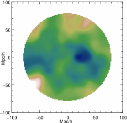
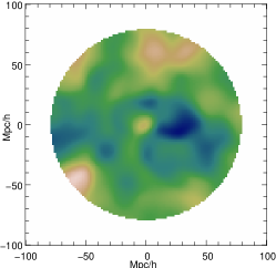
Real space reconstruction	Redshift reconstruction

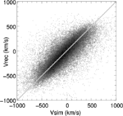
Figure 12: Redshift distortion correction – Top panels: A slice of the smoothed velocity field $v_{\text{r,sim}}$ and $v_{\text{r,rec}}$ is shown in the left and right panels, respectively. The two fields have been smoothed with a 5 $h^{-1}$Mpc Gaussian window, with objects put at their real (simulated and reconstructed) comoving coordinates. Bottom panels: Scatter plots between $v_{\text{r}}$ and $v_{\text{r,rec}}$ for individual mass tracers. The left panel (right panel) was produced using a real space reconstruction (redshift space reconstruction, respectively). In both cases, only objects within a sphere of 8000 km s^-1are shown.

Fig. 12 shows both reconstructed and simulated velocity fields and the scatter between $v^{\text{s}}_{\text{r,rec}}$ and $v_{\text{r,sim}}$. The first impression when comparing the two top panels of Fig. 12 is that the redshift reconstruction behaves really well. However, some potentially worrying localized features are present:

• Some important structures have their velocities badly reconstructed. Two important examples are the green-yellowish finger just above the center of the upper right panel of Fig. 12 and the big velocity peak at the top of this same panel. In the left panel, these two structures are not so prominent. The difference can be understood by studying the impact of the Kaiser effect on the reconstructed velocity field. Basically, two nearby filaments can merge in redshift space and give birth to a filament with a higher apparent density. The reconstruction is not able to separate these two filaments, which leads to an area with higher reconstructed velocities than the true ones. Thus, we expect in observational data to meet problems in the neighbourhood of the Great Wall, which is a supercluster of filaments compressed by redshift distortion.

• The velocity field in the immediate (5-10 $h^{-1}$Mpc) neighbourhood of the mock observer has lost its spatial structure and even presents a spurious peak. This is, most unfortunately, an expected problem that is linked to the above discussion on the problems of $I_{\sigma}$ near the observer. Indeed, in the neighbourhood of the observer, $I_{\sigma}$ becomes singular and the reconstruction misses, most likely, the right orbits. Analysing the smoothed velocity field seems to show that this effect looks in practice much like the one just above: the reconstructed velocity field may be boosted by the merging of different structures in the neighbourhood of the observer.

• The lower right panel presents two additional off-diagonal tails compared to lower left panel. As discussed earlier, these tails are due to shell-crossings occuring along the lines-of-sight when passing from real to redshift space. These extra shell-crossings result in some reconstructed velocities acquiring a sign opposite to the true velocities.

Similarly as in § 2, we have computed in Fig. 13 the distribution of differences $P^{\text{s}}_{\text{VE}}$ between $v^{\text{s}}_{\text{r,rec}}$ and $v^{\text{s}}_{\text{r,sim}}$, for a redshift reconstruction applied on 8k-mock6 based on a $64^{3}$ mesh. Though the distribution is of course wider than in Fig. 4, the previously drawn conclusions are still valid. $P^{\text{s}}_{\text{VE}}$ is better fitted by a Lorentzian distribution with $B=86$ km s^-1than by a Gaussian of width $\sigma=91$ km s^-1, particularly in the tails.

To check the effects of redshift distortion on the quality of the reconstruction, one can compare Table 3 to the first row of Table 1. As usual, the $s$ parameter is slightly biased below unity due to nonlinear effects discussed in § 2, which seem, not surprisingly, to be slightly enhanced by redshift distortions. The appeareance of the off-diagonal tails in the lower right panel of Fig. 12 increases the level of scattering, hence the correlation coefficient $r$ decreases and the signal-to-noise ratio increases. Reducing the analysis to the region inside 1.5$\sigma$ isocontour greatly improves the results, as expected, but still leads to a value of $\Omega_{\text{m}}$ slightly biased to lower values, $\Omega_{\text{m}}=0.27$.

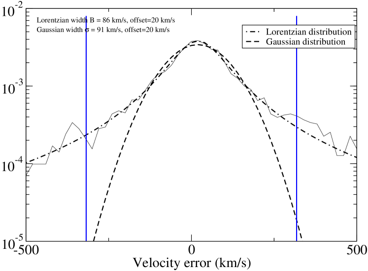
Figure 13: Error distribution of the reconstructed velocity field, redshift space – Same as in Fig. 4 but the solid curve corresponds to the probability distribution of the quantity $v^{\text{s}}_{\text{r,rec}}-v_{\text{r,sim}}$, where $v^{\text{s}}_{\text{r,rec}}$ and $v_{\text{r,sim}}$ are the line-of-sight reconstructed and simulated velocities, respectively.

5 Effects of catalogue geometry

In practice, real galaxy catalogues are not spatially periodic as is our simulation. They represent a region of finite volume with non-trivial geometry. In particular, two kinds of problems arise:

• Edge effects – Reconstruction of the galaxy trajectories without any piece of information on what may affect them dynamically from the outer parts of the catalogue is likely to introduce significant sources of errors, possibly systematic. We separate here edge effects into two subclasses: the effects of the obscuration by our galaxy, which defines a Zone of Avoidance (hereafter ZOA) and the effects of finite depth of the catalogue. These two effects need a separate treatment detailed in § 5.1 and § 5.2.

• Cosmic variance – The finite volume of the accessible part of the Universe might be a potentially unfair realization of the random process underlying the properties of the large scale matter distribution. We must investigate whether our method, including handling of edge effects, is robust to the recovering of the statistical properties of the whole Universe from observations of only a fraction of it.

5.1 Zone of avoidance

Dust present in the Milky Way’s galactic plane highly attenuates the light, thus galaxy catalogues generally do not provide any data in this direction (approximately the region within $|b|<5\;\deg$, where $b$ is the galactic latitude) of the ZOA. This strong attenuation introduces a boundary effect, which has the unpleasant feature of being present at any distance from the observer and may thus severely affect the measurements. As this area is nonetheless relatively small, particularly at low redshift, a simple correction should be able to greatly remove the boundary effect in the inner region of the catalogue.

Simulating the effect is made easy by putting an observer at the center of the simulation volume and by removing all mass tracers in the neighbourhood of the galactic plane $z=0$, i.e. which have $|b|<\alpha$. This gives us FullMockZOA.

Though more advanced ways of filling the ZOA exists (e.g., Lahav et al., 1994; Fontanot et al., 2003), this latter is here sufficiently small to be dealt with by the following simple algorithm. Since the statistical properties of the galaxies should not change across the boundaries of the ZOA, the objects in its neighbourhood can be used to fill the zone. We build new mass tracers to fill the obscured area by applying a locally planar symmetry transformation to the galaxies and groups with $-3\alpha<b<-\alpha$ according to the “plane” $-\alpha$. We execute the same operation on objects with $+\alpha<b<+3\alpha$ but according to the “plane” $+\alpha$. In the end, the masses of the copied haloes in the ZOA are divided by two and we only take half of the field galaxies. This method has been used previously to fill the zone of avoidance in NBG-3k (Shaya et al., 1995) and NBG-8k. This folding procedure has been applied to FullMockZOA, slightly moving some of the newly created objects to enforce the periodicity of the simulation box to avoid mixing the effect of the ZOA with other boundary effects. The results are presented in Fig. 14. As expected, the ZOA has a clear impact on errors of the reconstructed velocities.

The typical errors on the reconstructed velocities, represented in the left panel of this figure, rise substantially in the vicinity of the obscured area. Fortunately, they remain well below the natural velocity dispersion of the simulation (dashed line). As we are comparing velocity fields filtered with a 5 $h^{-1}$Mpc Gaussian window, we expect the reconstructed velocity field to be nearly error free for all points nearer than about 60 $h^{-1}$Mpc. It is also fortunate we have not introduced an extra bias using the filling algorithm, as shown both by comparing Table 4 to the first row of Table 1 and looking at the scatter plot in the right panel of the Fig. 14. We nonetheless highlight that the edge effect is not at all localized near the ZOA but extends quite far away and becomes negligible only for $|b|>20\;\deg$. Table 4 shows that the above extra noise does not have any impact on the measured $\Omega_{\text{m}}$.

Table 4: Zone of avoidance – Noise and biasing summary. Column description is given in the caption of Table 1.

$s$	$r$	$\sigma$	$\Omega_{\text{m}}$ ($s$)	$\Omega_{\text{m}}$ ($\mathfrak{L}_{\text{min}}$)	$\Omega_{\text{m}}$ ($\mathfrak{L}_{\text{max}}$)	$\Omega_{\text{m}}$ (1.5$\sigma$,$s_{\text{med}}$)	$\Omega_{\text{m}}$ (1.5$\sigma$,$s_{\text{min}}$)	$\Omega_{\text{m}}$ (1.5$\sigma$,$s_{\text{max}}$)
0.89	0.79	0.61	0.37	0.30	0.35	0.32	0.285	0.36

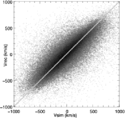
Figure 14: Zone of Avoidance / velocity field – Left panel: Binned average RMS (Root Mean Square) error on the smoothed velocity field. As usual, the velocity field window has been smoothed with a 5 Mpc/h Gaussian window. Each point is computed by averaging the square of the deviation of the velocity field along the line-of-sight and for all line-of-sights having belonging to the same $\sin(b)$ bin, where $b$ is the “galactic” latitude. The solid line gives the RMS error in the presence of a zone-of-avoidance at $b=0$. The dotted line gives the RMS error for a reconstruction on a catalogue without ZOA. The dashed line gives the RMS of the smoothed velocity field itself. Right panel: Scatter plots between $v_{\text{r,rec}}$ and $v_{\text{r,sim}}$ for individual mass tracers.

5.2 Lagrangian domain

Current density field
(a) TrueDom	(b) NaiveDom	(c) PaddedDom
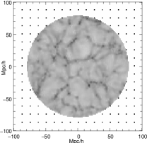
Reconstructed velocity fields
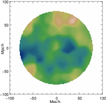
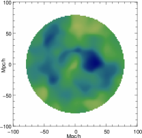
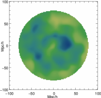
In 8000 km s-1
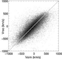
In 4000 km s-1

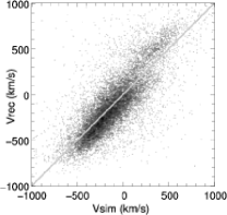
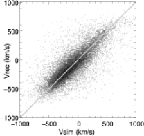
Figure 15: Lagrangian domain / without redshift distortions – This figure summarises the results obtained on reconstructions that have limited information on the Lagrangian domain. The left column illustrates the TrueDom reconstruction, The middle column the NaiveDom one, and the right column the PaddedDom one. For space occupation reasons, the original velocity field given by the simulation is not remembered but can be found in Fig. 11. The top row illustrates the three schemes for handling boundary effects on the density field: in the left column one retains information of large scale tidal fields, in the middle column one cuts the catalogue spherically and does a reconstruction on it, in the right column one pads the spherically-cut catalogue with particles homogeneously distributed on a grid. The second row gives the reconstructed velocity field in each case, smoothed with a 5 $h^{-1}$Mpc Gaussian window as usual. The color coding is the same as for the other figures, i.e. dark blue is -1000 km s^-1and white is +1000 km s^-1. The third row compares the individual (not smoothed) reconstructed and simulated velocities of objects in the 8k-mock6 catalogue. The fourth row does the same comparison but objects lying only in the 4000 km s^-1region of the 8k-mock6 catalogue.

Current density field
(a) TrueDom	(b) NaiveDom	(c) PaddedDom
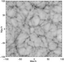
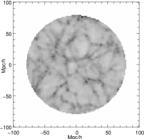
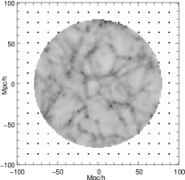
Reconstructed velocity fields
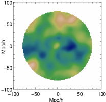
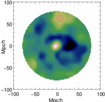
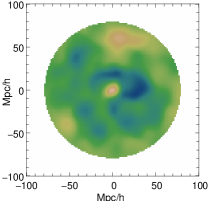
In 8000 km s-1
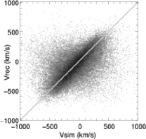
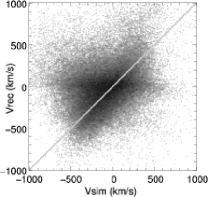
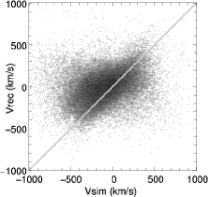
In 4000 km s-1

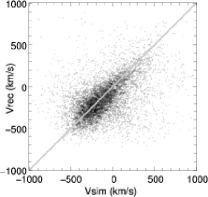
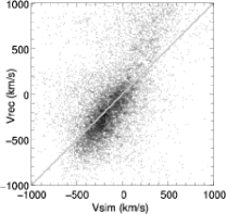
Figure 16: Lagrangian domain / with redshift distortions – Same as Fig. 15, but for mock catalogues including redshift distortion.

The inputs to MAK reconstruction are the present coordinates of the objects, i.e. ${\bf x}$ in Eq. (2) or ${\bf s}$ in Eq. (8), and the knowledge of the Lagrangian domain, i.e. ${\bf q}$ in Eq. (2) or (8). Redshift catalogues give the present “positions” of the objects, i.e. ${\bf s}$ in Eq. (8), however we have no observations that would give us the corresponding Lagrangian domain ${\bf q}$. We are thus limited to make guesses, though in the end, for huge catalogues, the details of the guess does not matter as gravitational forces are screened on large scales by the nearly homogeneous distribution of matter in the universe. Consequently, what happens at the boundaries should not strongly affect the central part of the catalogue though some guesses may be better at confining the edge effects on the boundaries. The naive solution is to assume that the Lagrangian domain is not so different from the volume of the catalogue itself. This assumption only begins to be a good approximation for volume enclosed in a sphere for which radius is big enough. For our 80 $h^{-1}$Mpc sample, the mass going in and out of the volume (from initial to present time) already represents about 16% of the total mass. For a 40 $h^{-1}$Mpc sphere, the mass flow is even greater: it may vary between 30% and 63 % of the total mass depending on the 8k-mock catalogue considered. Though tidal field and cosmic variance effects becomes negligible on a 80 $h^{-1}$Mpc scale, they still affect the boundaries of the Lagrangian domain of a given catalogue in a non-trivial way. As we shall show these problems are further enhanced by redshift distortion.

To achieve a meaningful comparison, we have run a reconstruction on 8k-mock6 using the Lagrangian domain given by the simulation; this reconstruction is called TrueDom. Now, we confront the results of TrueDom for two different reconstruction setups that try to recover the Lagrangian domain:

• NaiveDom reconstruction is obtained by assuming a naive spherical Lagrangian domain for 8k-mock6. In that case, all the mass that is presently in the 8k-mock6 catalogue was uniformly in a sphere of radius 80 $h^{-1}$Mpc. Equivalently, it means no significant mass flow must have gone through the comoving boundaries in the past.

• PaddedDom reconstruction is obtained by padding homogeneously the 8k-mock6 catalogue. The padding is chosen such that the final MAK mesh that will be reconstructed is an inhomogeneous cube (as in right panel of the second row of Fig. 15 and 16). The cube must be sufficiently big to absorb density fluctuations present at the boundary of the catalogue (typically a 20 $h^{-1}$Mpc buffer zone is needed). With real data, we are bound to assume that the catalogue is totally representative of the whole universe, i.e. its effective mean matter density is equal to $\Omega_{\text{m}}$.

Fig. 15 shows the result of a TrueDom, NaiveDom and PaddedDom reconstruction applied to 8k-mock6 in the absence of redshift distortion. Fig. 16 gives the same reconstructions when applied to a redshift catalogue. Table 5 summarises the value of the moments of $P(v_{\text{r,sim}},v_{\text{r,rec}})$ for different cases. We will now first confront the results of real space reconstructions, and second redshift space reconstructions.

TrueDom reconstruction does not yield any significant bias at 80 $h^{-1}$Mpc. However, at 40 $h^{-1}$Mpc, cosmic variance effects introduce a noticeable systematic error in the direction of higher $\Omega_{\text{m}}$ that will be discussed in § 5.3. Compared to TrueDom, NaiveDom gives good overall results though the central blue region of TrueDom turns to dark blue in NaiveDom, which would suggest the velocity field is biased. This analysis is confirmed by looking at the bottom scatter plot. The $\Omega_{\text{m}}$ measurement (Table 5) is underestimated by about 26% even in the central region of the catalogue which is normally less affected by boundary effects. PaddedDom, on the other hand, does not yield such a sharp discrepancy in the middle of 8k-mock6, namely in the 4k-mock6 region. Both the bottom scatter plot and the $\Omega_{\text{m}}$ measurement confirm that the reconstructed velocities are nearly bias-free in the central region. As expected, the velocities in the neighbourhood of the boundaries are completely wrong for the two methods.

Now, the catalogues are cut in redshift space. Redshift distortion biases the velocity distribution of objects on the catalogue boundary: the catalogue receive more infalling objects than outfalling ones. In some cases, one may even find objects seemingly artificially separated from the main volume of the catalogue (they look “disconnected”). In those cases, the hypothesis of convexity is definitely lost for those objects. This problem will enhance boundary problems. The case of TrueDom reconstruction has been discussed in § 4. As previously, the peculiar velocities in NaiveDom and in PaddedDom are largely uncorrelated in the full 8k-mock6 volume (Fig. 16). However, peculiar velocities reconstructed by NaiveDom are more strongly overestimated than by using PaddedDom’s, as shown in Table 5. For NaiveDom, the scatter is plagued by a horizontal alignment in Fig. 16, mid-lower panels, which is a signature of a strong edge effect. This spurious alignment was already present, though much less apparent, in the real space case. On the other hand, PaddedDom does not present this feature but only a large scatter. We have verified that objects belonging the horizontal alignment are essentially near the 80 $h^{-1}$Mpc boundary, contrarily to velocities reconstructed using PaddedDom which are more or less uniformly distributed and essentially uncorrelated to simulated velocities. This means that PaddedDom is at least better at screening edge effects than NaiveDom in the sense the errors are more evenly distributed and less systematic. Though impressively low in the last two rows of Table 5, the correlation coefficient $r$ is actually spoiled by the long tails of the PDF shown in the scatter plots in Fig. 16. Concerning $\Omega_{\text{m}}$, NaiveDom seems less robust to produce an unbiased estimation than PaddedDom. Indeed, looking at Table 5, one may note that the interval delimited by $s_{\text{med}}$, $s_{\text{min}}$ and $s_{\text{max}}$ nearly does not contain $\Omega_{\text{m}}=0.30$ for NaiveDom/Real space/40 $h^{-1}$Mpc, and does not contain it at all for NaiveDom/Redshift space. On the contrary, $\Omega_{\text{m}}=0.30$ is always selected by the three $s$ parameters using PaddedDom reconstruction. In the rest of this paper, whenever it is needed, we will thus use the PaddedDom reconstruction.

Table 5: Lagrangian volume – Residual error after the correction. Description for some columns is given in the caption of Table 1. “Radius” gives the spatial size of the sphere on which the velocity-velocity comparison is conducted. “Reconstruction type” indicates the type of Lagrangian domain reconstruction and whether it is mixed with redshift distortion effect. Details on the meaning of each name are given in § 5.2.

Reconstruction type	Radius ($h^{-1}$Mpc)	Velocities			$\Omega_{\text{m}}$ ($s$)	$\Omega_{\text{m}}$ ($\mathfrak{L}_{\text{min}}$)	$\Omega_{\text{m}}$ ($\mathfrak{L}_{\text{max}}$)	$\Omega_{\text{m}}$ (1.5$\sigma$,$s_{\text{med}}$)	$\Omega_{\text{m}}$ (1.5$\sigma$,$s_{\text{min}}$)	$\Omega_{\text{m}}$ (1.5$\sigma$,$s_{\text{max}}$)
		$s$	$r$	$\sigma$
TrueDom / Real space	80	0.91	0.77	0.66	0.35	0.28	0.31	0.27	0.233	0.32
	40	0.80	0.76	0.65	0.45	0.28	0.38	0.35	0.28	0.43
NaiveDom / Real space	80	0.87	0.52	0.92	0.38	0.20	0.28	0.42	0.20	0.87
	40	1.11	0.77	0.73	0.25	0.20	0.24	0.244	0.19	0.31
PaddedDom / Real space	80	0.73	0.65	0.77	0.53	0.36	0.48	0.45	0.27	0.75
	40	0.91	0.77	0.64	0.35	0.28	0.34	0.32	0.26	0.38
NaiveDom / Redshift space	40	1.49	0.51	1.31	0.11	0.15	0.26	0.20	0.12	0.37
PaddedDom / Redshift space	40	0.93	0.53	0.94	0.36	0.18	0.34	0.38	0.20	0.79

5.3 Cosmic variance

8k-Mock6	8k-Mock7	8k-Mock12

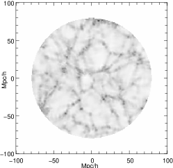
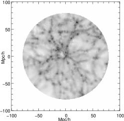
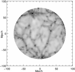
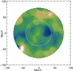
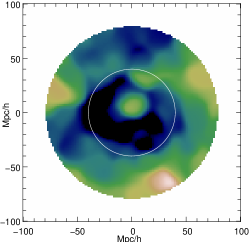
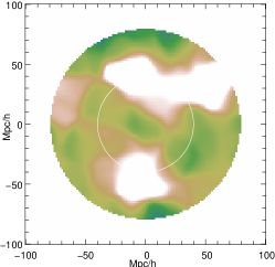
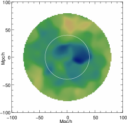
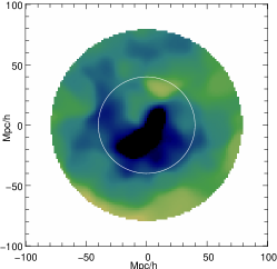
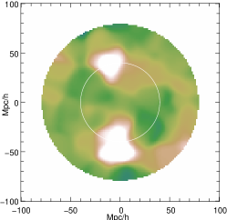
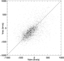
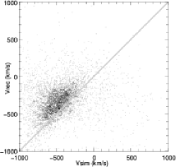
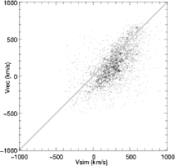
Figure 17: Cosmic variance – This figure gives a visual comparison of the three mock catalogues used to study cosmic variance effects. Top panels: Adaptively smoothed density fields of the considered mock catalogues. In each case, we have represented the central thin slice that contains the observer. Second row: Simulated velocity field, after smoothing with a 5 $h^{-1}$Mpc Gaussian window. The white circle gives the limit of the 40 $h^{-1}$Mpc volume. Third row: Same as second row, but for the reconstructed velocity field. Fourth row: Comparison between reconstructed and simulated peculiar velocities.

We generally assume that galaxy catalogues give a fair representation of the whole universe, but of course we have no guarantee that this assumption is correct. Thus, the result of a MAK reconstruction may be affected by inhomogeneities above the catalogue scale. For instance, our galaxy may reside in a particularly extreme region (overdense or underdense), which would produce unusual peculiar velocities. This effect, known as cosmic variance, can be investigated by our three original basic mock catalogues: 4k-mock6, 4k-mock7, 4k-mock12 (§ 1). The cosmic variance effect is here further enhanced by the finiteness of the sampled volume. The volume is sufficiently small here to have a non-zero average line-of-sight velocity. On a 40 $h^{-1}$Mpc scale, this effect can substantially modify the $\Omega_{\text{m}}$ measurement (put $\Omega_{\text{m,mes}}$ in this section) by cutting the $P(v^{s}_{\text{rec}},v_{\text{sim}})$ distribution at an inadequate place.

Table 6: Cosmic variance – Summary of measurements conducted on the three mock catalogues. The reconstruction is either conducted on the basic catalogue without any observational effect besides cosmic variance (labelled Original), or on the same catalogue but affected by redshift distortion, incompleteness and for which the Lagrangian domain is determined using PaddedDom (reconstruction labelled Full). The description of the other columns are given Table 1.

Catalog	Reconstruction type	Velocity field			$\Omega_{\text{m}}$ ($s$)	$\Omega_{\text{m}}$ ($\mathfrak{L}_{\text{min}}$)	$\Omega_{\text{m}}$ ($\mathfrak{L}_{\text{max}}$)	$\Omega_{\text{m}}$ (1.5$\sigma$,$s_{\text{med}}$)	$\Omega_{\text{m}}$ (1.5$\sigma$,$s_{\text{min}}$)	$\Omega_{\text{m}}$ (1.5$\sigma$,$s_{\text{max}}$)
		$s$	$r$	$\sigma$
4k-mock6 ($\Omega_{\text{eff}}=0.35$)	Original	0.80	0.76	0.65	0.313	0.28	0.38	0.35	0.28	0.43
	Full	0.94	0.50	0.96	0.35	0.13	0.31	0.31	0.16	0.70
4k-mock7 ($\Omega_{\text{eff}}=0.5$)	Original	0.70	0.67	0.76	0.57	0.39	0.47	0.40	0.33	0.48
	Full	0.88	0.11	1.33	0.43	0.41	1.62	0.30	0.09	1.29
4k-mock12 ($\Omega_{\text{eff}}=0.19$)	Original	1.12	0.81	0.66	0.24	0.235	0.27	0.24	0.22	0.26
	Full	1.08	0.58	1.11	0.24	0.29	0.62	0.15	0.08	0.31

The results of the reconstruction on these three mock catalogues are given in Fig. 17. In Table 6, we give, for each mock catalogue, the best achievable result (thus highlighting purely the effect of choosing this mock catalogue) and the results one would obtain through observation of this piece of the universe. Unknown Lagrangian domain, redshift distortion and incompleteness effects are added to the considered mock catalogue. The problems of mass-to-light assignment and the zone of avoidance are left apart for the sake of clarity. Their imprint on the velocities should most likely remain the same as we have shown in the corresponding previous sections, i.e. biasing for the first and increase of the scatter for the second. Only the cases with the forementioned observational effects are represented in Fig. 17.

Visual inspection of lower scatter plots in Fig. 17 shows that volume finiteness is likely making the $\Omega_{\text{m,mes}}$ measurement sensitive to the “local” $\Omega_{\text{m}}$ ($\Omega_{\text{eff}}$ in the table). This assertion is supported by the estimation of $s$ and $\Omega_{\text{m}}$ for TrueDom reconstructions given in Table 6. Moreover, experiments conducted with the spherical collapse model show that $\Omega_{\text{m,mes}}$ is indeed a weighted average between $\Omega_{\text{eff}}$ and $\Omega_{\text{m}}$.

More specifically, reconstructed velocities in 4k-mock7 (including observational effects) are apparently giving the $\Omega_{\text{m}}$ of the simulation but they present a large scatter rendering the slope estimation dubious. Indeed, doing the same reconstruction but without observational effects give a measured $\Omega_{\text{m,mes}}=0.40$, which is the exact average between the simulation $\Omega_{\text{m,simu}}=0.30$ and $\Omega_{\text{eff}}=0.50$. The aforementioned scatter is expected for this mock catalogue: the velocity field is badly reconstructed near the observer in that case (middle panels) because the local cosmic flow is higher than usual ($\sim$1000 km s^-1) and the non-linearities are stronger. Thus the convexity of the problem is lost on an extended region around the observer when the reconstruction is conducted in redshift space (see § 4). A particularly saliant misreconstruction is given by the outflowing “bubble” at the center which disappears in the reconstructed velocity field. The size of the affected region is about 20 $h^{-1}$Mpc around the observer in 4k-mock7 and thus limits the number of objects having both good reconstructed and observable peculiar velocities.

In an opposite way, velocities in 4k-mock12 are reconstructed with a better correlation, as shown by Table 6, but $\Omega_{\text{m}}$ measurement is strongly weighted toward $\Omega_{\text{eff}}$. These two “features” are largely due to the huge central void. First, MAK reconstruction and Zel’dovich approximation are known to work better in low density regions and being centered on a void results in inhibiting blueshift distortion as galaxies are principally going away from the observer, rendering the reconstruction problem convex in Eq. (8). Second, the low density region largely affects the statistical velocity distribution, which in this case leads to a measured $\Omega_{\text{m,mes}}$ weighted more strongly towards the $\Omega_{\text{eff}}$ of 4k-mock12. This leads us to a $\Omega_{\text{m,mes}}$ that is nearer $\Omega_{\text{m,simu}}$ in 4k-mock12 than the mean matter density of the whole simulation. The volume finiteness also produces an apparent offset between reconstructed velocities and measured ones. This is expected as doing a statistical analysis on a finite volume catalogue must introduce a selection bias effect. We have indeed checked that the point set $\left\{(v_{\text{r},i},\psi^{\text{s}}_{\text{r},i})\right\}$, obtained through a MAK reconstruction applied on 4k-mock12, is a subset of the corresponding set built from a reconstruction on 8k-mock12. Looking at our “standard” 4k-mock6, one can note that the simulated velocity distribution is generally more symmetric according to the null velocity than for the two other mock catalogues, with no visual bias while comparing reconstructed velocity to simulated velocity. This supports the initial assertion linking $\Omega_{\text{m,mes}}$ to $(\Omega_{\text{m,simu}},\Omega_{\text{eff}})$ and the asymetric distribution of velocities. Potentially, one could recover the true $\Omega_{\text{m}}$ of the Universe (or here the simulation) from the measured velocities of any catalogues by predicting how the velocity distribution asymmetry is linked to local density contrast. However, the simplest, and more robust solution, would still be to extend the depth of current catalogues to reach a volume where velocities are normally distributed.

From a prediction point of view, comparing visually the velocity fields inside the white circles show that, if we know $\Omega_{\text{m}}$, we reconstruct plausible velocity fields for the three mock catalogues. Outside the white circles, the reconstructed velocity field is nearly completely uncorrelated compared to the simulated one as we have discussed in the previous section. It must be noted that the velocity field goes smoothly to zero (green colour) on the edge of all mock catalogues: this is an expected side effect of the homogeneous padding which tends to smooth out any fluctuation on the edge (velocity and density field).

6 Velocity measurement errors

6.1 The need for a likelihood analysis ?

All the effects already described in this paper are present in a redshift catalogue. Though we expect most of the observational biases should be independent, some of them may correlate and give worse systematic errors. We present in Fig. 18 the progressive deterioration of the velocity-velocity comparison for 4k-mock6 based on a reconstruction conducted on 8k-mock6. The effects are piled up from left to right. The $\Omega_{\text{m}}$ measurements for the 1.5$\sigma$ method are indicated below each panel. The obvious conclusion is that the measurements are progressively affected but that no extra correlated error seems to happen when mixing the effects. Another fortunate event is that bias seems to counterbalance themselves to give in the end a nearly unbiased result (last but one panel). Going from TrueDom/Real to Redshift tends to decrease $\Omega_{\text{m}}$ as has been seen previously. On the contrary, injecting incompleteness pushes the measurement to higher $\Omega_{\text{m}}$ as we have noticed in § 3.3. The 1.5$\sigma$ method seems to give the right $\Omega_{\text{m}}$ value in all cases, which means that we should be able to use it on galaxy catalogues provided we have sufficient precision on velocity measurements. However, looking at the last panel (bottom right) of Fig. 18 shows that injecting random velocity measurement errors (here we intruduced an optimistic error of 8% of the distance to the object, corresponding to an error on distance modula of $\sigma_{\mu}=0.17$), renders slope estimation much more difficult. In that case, the measured $\Omega_{\text{m}}$ is severely biased. This is expected as the 1.5$\sigma$ method relies mostly on the central part of the scatter, which in turn is the one that is the most affected by random errors. This leads to a circularization of the 1.5$\sigma$ isocontour and thus a completely wrong estimation of the slope. On the other hand, looking at the global structure of the scatter shows that the right slope is still hidden in the data, but one should then take into account the tails of the distribution. This last test shows the limit of a direct velocity-velocity comparison in real cases. It might be possible to recover the original distribution of the scatter by deconvolving from the noise. However, it seems to be a difficult operation and we prefer to first try a maximum likelihood approach. Its main advantage would be to work using distances, thus rendering the error in measurements more tractable.

	Cosmic variance	Lagrangian domain	Redshift distortion
$\mathfrak{L}$	$\Omega_{\text{m}}=[0.28,0.38]$	$\Omega_{\text{m}}=[0.28,0.34]$	$\Omega_{\text{m}}=[0.18,0.34]$
1.5$\sigma$	$\Omega_{\text{m}}=[0.28,0.35,0.43]$	$\Omega_{\text{m}}=[0.26,0.32,0.38]$	$\Omega_{\text{m}}=[0.15,0.30,0.68]$
	Incompleteness	Observational errors ($\sigma_{\mu}=0.17$)
$\mathfrak{L}$	$\Omega_{\text{m}}=[0.13,0.31]$	$\Omega_{\text{m}}=[0.10,0.30]$
1.5$\sigma$	$\Omega_{\text{m}}=[0.20,0.38,0.79]$	$\Omega_{\text{m}}=[0.08,0.78,1]$

Figure 18: This figure gives the evolution of the scatter distribution and of the measurement of $\Omega_{\text{m}}$ using it while more and more observational effects are added to 8k-mock6 catalogue. All measurements of $\Omega_{\text{m}}$ are given between brackets and are sorted as follows. For measurements obtained through the likelihood analysis, labelled by $\mathfrak{L}$, the first number corresponds to $\mathfrak{L}_{\text{min}}$ and the second to $\mathfrak{L}_{\text{max}}$. For measurements obtained using the 1.5$\sigma$ method, the first number corresponds to $s_{\text{min}}$, then $s_{\text{med}}$ and finally $s_{\text{max}}$. The last (lower right) panel uses the full likelihood function of Eq. (31). All others use a restricted likelihood analysis with $\sigma_{0}/e=0$, which is nearly equivalent to using Eq.(30) for each $(v_{\text{r},i},\psi_{\text{r};i})$ pair. The $1.5\sigma$ isocontour has been plotted with a thick dashed line in the last panel.

6.2 Maximum likelihood analysis

Observations of galaxies first give us access to their distances and not their peculiar velocities. A method based on distances to make a comparison between a model and observations is potentially less sensitive to distance measurement errors. Indeed, by comparing directly distances, one has a small relative error on each measurement instead of a huge one when peculiar velocities are considered. Below, we discuss galaxy selection bias and zero-point calibration errors in distance measurements while keeping the notation of Strauss & Willick (1995).

Presentation of the Bayesian chain – For the Tully-Fisher (TF) relation, one makes an estimate of the absolute magnitude of a galaxy as a function of its linewidth: the slope between the two quantities can be biased because the sample is limited in magnitude (Strauss & Willick, 1995). This effect which is known as selection bias is purely statistical and if not correctly taken into account can lead to large systematic errors. Using these absolute magnitudes, occasionally combined to form groups of galaxies, and the apparent magnitudes of the same group, one builds the distance modulus

$$\mu(r)=m(r)-M=5\log_{10}\left(\frac{r}{10~{}pc}\right)$$ (10)

with $r$ the distance of the considered object (group of galaxies or galaxy). In addition to the forementioned statistical bias, peculiar velocity obtained from redshift positions through a Lagrangian reconstruction, here MAK, are sometimes very noisy, as shown in Fig. 18. Another more subtle effect is introduced by the Gaussian distribution of our velocity sample that we are going to analyze. We need to take care of this “selection bias” to avoid being spoiled by eventual large reconstruction errors present for objects with a high velocity. Thus we need a Bayesian approach to account for all these statistical effects.

In principle, the likelihood function gives a probability for the data, i.e. here redshift positions $\mathfrak{Z}=\{{\bf z}_{i}\}$, with $i$ running from 1 to $N$, and distance moduli $\mathfrak{M}=\{\mu_{i}\}$, assuming some model described by the vector parameter $p$. Additionally we assume that we have an estimation of measurement errors on $\mathfrak{M}$ through the set $\mathfrak{S}$. The exact description of $\mathfrak{S}$ will be given in the next paragraph. Typically errors on redshift measurements are of the order of 50-60 km s^-1. This means that we can consider them as negligible if we consider objects farther than $R_{z}=6-10$ $h^{-1}$Mpc. The volume enclosed by the sphere of radius $R_{z}$ is, in any case, also poorly reconstructed because of the singularity introduced by redshift distortions near the observer (§ 4). In the following analysis, we will consider redshift measurements as negligible by avoiding the objects located at less that 10 $h^{-1}$Mpc from the observer, thus we have:

$$P(\mathfrak{M},\mathfrak{Z}|p,\mathfrak{S})\propto P(\mathfrak{M}|\mathfrak{Z},p,\mathfrak{S})=\mathfrak{L}(p)$$ (11)

The end of this section is devoted to computing the right hand part of this equation. To achieve this, we will decompose the probability into small pieces:

$$P(\mathfrak{M}|\mathfrak{Z},\mathfrak{S},p)=\\ \iiint\limits_{\mathfrak{M}_{r},\mathcal{V},D}P(D)P(\mathfrak{M}|\mathfrak{M}_{r},\mathfrak{S},D,p)\\ \times P(\mathfrak{M}_{r}|\mathcal{V},\mathfrak{Z},p)P(\mathcal{V}|\mathfrak{Z},p)\;\text{d}\mathfrak{M}_{r}\text{d}\mathcal{V}\text{d}D$$ (12)

with $\mathfrak{M}_{r}=\{\mu_{1,r},\ldots,\mu_{N,r}\}$ representing the “true” distance moduli, with $\mu_{i,R}\in[-\infty,+\infty]$ and $\mathcal{V}=\{v_{1},\ldots,v_{n}\}$ the “true” object peculiar velocities. $P(\mathfrak{M}|\mathfrak{M}_{r},\mathfrak{S},p)$ is the probability of measuring the set of distance moduli $\mathfrak{M}$ given that the real set of distance moduli is $\mathfrak{M}_{r}$ and the expected error on the measurement is given by $\mathfrak{S}$. $P(\mathfrak{M}_{r}|\mathcal{V},p)$ is the probability of obtaining the set of distance moduli $\mathfrak{M}_{r}$ given the reconstructed velocities $\mathcal{V}$. $P(\mathcal{V}|\mathfrak{Z},p)$ is the probability the velocities are well reconstructed from the redshift data $\mathfrak{Z}$. The probability $P(D)$ is going to be introduced in the last paragraph to account for uncertainty in the calibration of the Tully-Fisher relation. All those probabilities are computed assuming the model parameters $p$. We will establish the likelihood function $\mathfrak{L}(p)$ in three steps:

• First, the error distributions linked to observations are considered to get an unbiased distance estimator for groups. This analysis yields the probability $P(\mu_{i}|\mu,\sigma_{\mu,i},p)$.

• Second, the errors on reconstructed velocities are considered to compute $P(v|\mathfrak{Z},p)$.

• Last, the two analyses are merged as given above to produce the likelihood function which gives the posterior distribution of $\beta$ and the Hubble constant $H$.

A picture of the above Bayesian chain is given in Fig. 19.

Figure 19: Maximum likelihood analysis – This sketch illustrates the bayesian chain used to establish the likelihood function. The input data are located on the left and the output posterior distribution $P(\beta,H)$ on the right.

Distance modulus error distribution – To establish the likelihood function comparing the measured distance to the reconstructed velocity field, we assume the distance catalogues are obtained using the inverse TF relation (Shaya et al., 1995),

$$\eta^{0}(M)=-e(M+D)\;,$$ (13)

where $M$ is the absolute magnitude of the considered galaxy, $\eta_{0}(M)$ is its predicted linewidth, $e$ is the slope, and $D$ is the zero point calibration (the latter two are assumed to be known exactly). It is known that inverse TF is less sensitive to the selection bias as compared to forward TF (Strauss & Willick, 1995). Observational data show that the differences between the predicted linewidth $\eta^{0}(M)$ and the measured linewidth $\eta$ for an object of absolute magnitude $M$ are Gaussian distributed (Pizagno et al., 2006; Tully & Pierce, 2000). Thus, the probability of measuring the linewidth $\eta$, given that the object has an absolute magnitude $M$, and assuming that the TF relation $\eta^{0}(M)$ is known, is

$$P(\eta|M,e,D)=\frac{1}{\sqrt{2\pi}\sigma_{\eta}(M)}\mathrm{e}^{-\frac{\left(\eta-\eta^{0}(M)\right)^{2}}{\sigma_{\eta}^{2}(M)}}$$ (14)

with $\sigma_{\eta}(M)$ the linewidth estimation error for the absolute magnitude $M$. Distance catalogues are composed of estimated distance moduli $\mu_{e}$ from the inverse TF relation. These estimated distance moduli are built from the statistics on a single group. Therefore, the joint probability of having a galaxy in a group with both a linewidth $\eta$ and an absolute magnitude $M$, assuming the TF relation $\eta^{0}(M)$, is:

$$P(\eta,M|e,D)=F(M)P(\eta|M,e,D)\;,$$ (15)

where $F(M)$ is the normalized absolute luminosity function of the group.

The estimator for the distance modulus is given by:

$$\mu_{e}=m-M_{e}(\eta)=M+\mu_{0}(r)+D^{\prime}+\frac{\eta}{e^{\prime}}\;,$$ (16)

where $D^{\prime}$ and $e^{\prime}$ are the estimated inverse TF parameters of Eq. (13) and $\mu_{0}(r)=5\log(\frac{r}{10pc})$ the true distance modulus of the considered group. The conditional probability that the estimated distance modulus for the group is $\mu$, assuming that the estimated Tully-Fisher parameters are $e^{\prime}$ and $D^{\prime}$ and that the real parameters for this group are $e$ and $D$, can be written as

$$P(\mu|\mu_{0}(r),e,e^{\prime},D,D^{\prime})=\left\langle\delta_{\text{D}}\left(\mu-\mu_{e}\right)\right\rangle_{\text{group}}\\ =\left\langle\delta_{\text{D}}\left(\mu-\mu_{0}(r)+M+D^{\prime}+\frac{\eta}{e^{\prime}}\right)\right\rangle_{\text{group}}\\ =\int\limits_{M}\frac{e^{\prime}F(M)}{\sqrt{2\pi}\sigma_{\eta}(M)}\mathrm{e}^{-\frac{\left(e^{\prime}(\mu_{0}(r)-\mu)+e^{\prime}D^{\prime}-eD+(e^{\prime}-e)M\right)^{2}}{2\sigma_{\eta}^{2}(M)}}~{}dM\,.$$ (17)

While working with the inverse TF relation, one can assume that the slope $e^{\prime}$ is completely determined and $e^{\prime}=e$. Since the observed $\sigma_{\eta}(M)$ varies little with $M$, it is chosen to be equal to a constant $\sigma_{0}$. The previous probability reduces to

$$P(\mu|\mu_{0}(r),e,D,D^{\prime},\sigma_{0})=\frac{e}{\sqrt{2\pi}\sigma_{0}}\mathrm{e}^{-e^{2}\frac{\left(\mu-\mu_{0}(r)+D^{\prime}-D\right)^{2}}{2\sigma_{0}^{2}}}\text{.}$$ (18)

Though the slope $e^{\prime}$ is well determined, the zero-point calibration $D$ may still be affected by non-negligible errors. The set describing errors on distance moduli is thus $\mathfrak{S}=\{\sigma_{0,1}/e,\ldots,\sigma_{0,N}/e\}$$=\{\sigma_{\mu,1},\ldots,\sigma_{\mu,N}\}$. The error on this calibration will affect the distances globally. As a first approximation we model the error on the zero point by a Gaussian centered on $D$ with a standard deviation of $\sigma_{\text{\sc d}}$.

Linking distance modulus to velocity – The second probability function in Eq. (12) is $P(\mathfrak{M}_{r}|\mathcal{V},\mathfrak{Z},p)$, which is actually a distribution linking the velocities and redshifts to distance modulus. This principally corresponds to a change of variable and we give directly the expression of it, which is inspired by Eq. (1):

$$P(\mathfrak{M}_{r}|\mathcal{V},\mathfrak{Z},p)=\\ \prod\limits_{i=1}^{N}H10^{\mu_{r,i}/5}\delta_{\text{D}}\left(z_{i}-v_{i}-10\text{ pc}\times H10^{\mu_{r,i}/5}\right)$$ (19)

Reconstructed velocity distribution – We are now going to establish the expression of $P(v|\mathfrak{Z},p)$ with the vector of parameters of our chosen model $p=(H,\beta,B_{v},\sigma_{v},\gamma_{*},e)$ – $\sigma_{v}$ and $\gamma_{*}$ are going to be introduced in the next immediate paragraphs. One may decompose $P(v|\mathfrak{Z},p)$ that way

$$P(v|\mathfrak{Z},p)=\int_{\mathfrak{P}}P(v|\mathfrak{P},p)P(\mathfrak{P}|\mathfrak{Z},p)\;\text{d}\mathfrak{P}\,,$$ (20)

with $\mathfrak{P}=\{\psi_{r,i}\}$ the reconstructed displacements. As MAK reconstruction is deterministic once $\beta$ has been assumed (§ 4), the second probability distribution is simply given in our case by

$$P(\mathfrak{P}|\mathfrak{Z},p)=\prod\limits_{i=1}^{n}\delta_{\text{D}}\left(\psi_{r,i}-\psi_{i}\left(\mathfrak{Z},\beta\right)\right)$$ (21)

with $\psi_{i}$ representing the MAK reconstructed displacement of the $i$-th object, being a function of all redshift coordinates and $\beta$. Thus, studying $P(\mathcal{V}|\mathfrak{Z},p)$ reduces to examine $P(\mathcal{V}|\mathfrak{P}(p_{0}),p^{\prime})$, with $p^{\prime}=(H,\beta^{\prime},B_{v},\sigma_{v},\gamma_{*})$, $p_{0}=(H,\beta_{0},B_{v},\sigma_{v},\gamma_{*})$, $\beta_{0}$ being the assumed growth factor to compute the set $\mathfrak{P}(p_{0})$ using the redshift reconstruction. $P(\mathcal{V}|\mathfrak{Z},p)$ and $P(\mathcal{V}|\mathfrak{P}(p_{0}),p^{\prime})$ equalizes only if $p=p^{\prime}=p_{0}$. Thus one needs a several redshift reconstructions to build the probability function $P(\mathcal{V}|\mathfrak{Z},p)$. Working with the intermediary set $\mathfrak{P}$ is easier than with $\mathfrak{Z}$, we thus put the reduced likelihood function:

$$\mathfrak{L}^{\prime}_{\beta_{0}}(p^{\prime})=\\ \iint\limits_{\mathfrak{M}_{r},\mathcal{V}}P(\mathfrak{M}|\mathfrak{M}_{r},\mathfrak{S})P(\mathfrak{M}_{r}|\mathcal{V},\mathfrak{Z},p)P(\mathcal{V}|\mathfrak{P}(p_{0}),p^{\prime})\;\text{d}\mathfrak{M}_{r}\text{d}\mathcal{V}$$ (22)

and we are going to establish the expression of the elementary probability function $P(v_{r}|\psi_{r},p)$ which will yield

$$P(\mathcal{V}|\mathfrak{P}(p_{0}),p)=\prod\limits_{i=1}^{N}P(v_{r,i}|\psi_{r,i},p)$$ (23)

assuming statistical independance of all $\{v_{r,i},\psi_{r,i}\}$ duets, and that $\mathfrak{P}(p_{0})$ is obtained using a redshift reconstruction for which $\beta=\beta_{0}$. $\mathfrak{L}^{\prime}$ may be written in a factorized way:

$$\mathfrak{L}^{\prime}_{\beta_{0}}(p^{\prime})=\\ \prod\limits_{i=1}^{N}\,\,\iint\limits_{\mu_{r},v_{r}}P(\mu_{i}|\mu_{r},\sigma_{0,i}/e)P(\mu_{r}|v_{r},z_{i},p)P(v_{r}|\psi_{r,i},p)\;\text{d}\mu_{r}\text{d}v_{r}\text{.}$$ (24)

The computation of $\mathfrak{L}^{\prime}$ is clearly helped using this factorized form. We may now concentrate on the third probability function of the above equation.

As has been established in § 2, the distribution of errors on the reconstructed velocity field is the Lorentzian

$$P_{\text{DE}}(e_{\psi v})\propto\frac{1}{1+\left(\frac{e_{\psi v}}{B_{v}}\right)^{2}}\text{,}$$ (25)

where $B_{v}=86$ km s^-1(redshift reconstruction), with $e_{\psi v}$ the distance between the reconstructed velocity $\beta\Psi_{r}$ and the true velocity $v_{r}$. This formulation is different from saying that the reconstructed velocity is affected by error when compared to the true velocity, and permits some errors in the MAK reconstructed displacement field. As has been seen in § 5.3, the reconstructed velocities may also contain an extra offset that needs to be removed while measuring $\beta$. The error distance $e_{\Psi v}$ is thus

$$e_{\Psi v}=\alpha_{*}v_{r}-\beta_{*}\Psi_{r}+\gamma_{*}$$ (26)

with

$$\alpha_{*}^{2}+\beta_{*}^{2}=1\text{ and }\beta=\beta_{*}/\alpha_{*}$$ (27)

and $\gamma_{*}$ to account for a potential spurious offset in reconstructed velocities. From linear theory (Peebles, 1980), we know that the line-of-sight component of the velocity field must be distributed like a Gaussian function. We now assume that the absolute probability for an object to have a velocity $v$ is given by a Gaussian distribution:

$$P_{\text{vel}}(v|p)=\frac{1}{\sqrt{2\pi}\sigma_{v}}\mathrm{e}^{-\frac{v^{2}}{2\sigma_{v}^{2}}}\text{.}$$ (28)

It must be noted that it is likely that the observational data does not encompass a sufficiently large volume so that measured velocities follow this law. Moreover, this prior is of some importance when we have to deal with highly scattered data. The shortcomings of such an approach will be discussed in the next section. One can recover the standard uniform prior on velocities by taking the limit $\sigma_{v}\rightarrow+\infty$ in the next equations. Assuming $e_{\psi v}$, as a random variable, is independent of $v_{r}$ and these two quantities are themselves statistically independent from $\beta$ and $\gamma_{*}$, we may now write the joint probability of reconstructing $\psi_{r}$, having a true velocity $v_{r}$:

$$P(v_{r},\psi_{r},\beta,\gamma_{*}|B_{v},\sigma_{v})\\ ={\beta_{*}P_{\text{DE}}(e_{\Psi v}|B_{v},\sigma_{v})\times}\\ P(\beta,\gamma_{*}|B_{v},\sigma_{v})P(v_{r}|B_{v},\sigma_{v})P(\psi_{r}|B_{v},\sigma_{v})\\ =\beta_{*}C(B_{v},\sigma_{v})P(\beta,\gamma_{*}|B_{v},\sigma_{v})\frac{P(\psi_{r}|B_{v},\sigma_{v})\,\mathrm{e}^{-\frac{v_{r}^{2}}{2\sigma^{2}_{v}}}}{1+\left(\frac{\beta_{*}\psi_{r}-\alpha_{*}v_{r}+\gamma_{*}}{B_{v}}\right)^{2}}\,,$$ (29)

where $C$ is a function eventually depending on $B_{v}$ and $\sigma_{v}$. The conditional probability that the true velocity is $v_{r}$ given the reconstructed displacement $\psi_{r}$ is now exactly

$$P(v_{r}|\psi_{r},p)=\\ \frac{\mathrm{e}^{-\frac{v_{r}^{2}}{2\sigma^{2}_{v}}}\left(1+\left(\frac{\beta_{*}\psi_{r}-\alpha_{*}v_{r}+\gamma_{*}}{B_{v}}\right)^{2}\right)^{-1}}{\int_{v=-\infty}^{+\infty}\mathrm{e}^{-\frac{v^{2}}{2\sigma^{2}_{v}}}\left(1+\left(\frac{\beta_{*}\psi_{r}-\alpha_{*}v+\gamma_{*}}{B_{v}}\right)^{2}\right)^{-1}\;\text{d}v}\;.$$ (30)

The denominator of the right hand part of this equation must be computed numerically. It can be shown that, in the limit $\sigma_{v}\rightarrow+\infty$, $P(v_{r}|\psi_{r},\beta_{*},\gamma_{*})$ reverts to a pure Lorentzian form.

Merging the probability distributions – We may now establish the “elementary” conditional probability for an object $i$ to get a measured distance $\mu_{i}$ given that its reconstructed displacement is $\psi_{r,i}$, its redshift is $z_{i}$, the error on the linewidth measurement is $\sigma_{0,i}$ and the model parameters are $p^{\prime}$ in the notation of this section:

$$P(\mu_{i}|\psi_{r,i}(p_{0}),z_{i},\sigma_{0,i},D^{\prime},p^{\prime})\\ =\iint\limits_{v,\mu_{r}}P(\mu_{i}|\mu_{r},\sigma_{0,i},D^{\prime},p^{\prime})P(\mu_{r}|v,z_{i},p^{\prime})\\ \times P(v|\psi_{r,i}(p_{0}),p^{\prime})\;\mathrm{d}\mu_{r}\mathrm{d}v\\ \propto\frac{eH}{\sigma_{0,i}}\int_{\mu_{r}}10^{\mu_{r}/5}\text{e}^{-\frac{e^{2}}{2\sigma^{2}_{0,i}}\left(\mu_{r}-\mu_{i}+D-D^{\prime}\right)^{2}}\\ \times P\left(v=(z_{i}-10\text{ pc}\times H10^{\mu_{r}/5})|\psi_{r,i}(p_{0}),p^{\prime}\right)\;\mathrm{d}\mu_{r}\text{,}$$ (31)

with $p^{\prime}=(H,\beta^{\prime},B_{v},\sigma_{v},\gamma_{*})$, $\psi_{r,i}(p_{0})$ being computed assuming the parameters $p_{0}$. Looking closely at this probability, one may notice that changing $D\rightarrow D^{\prime}=D+\Delta$ is equivalent to changing $H\rightarrow H^{\prime}=H\,\text{exp}(\Delta/5)$. Thus the uncertainty in the zero point calibration translates only in an uncertainty on $H$ and not on the parameters of the model.

We may now write the full formal expression of $\mathfrak{L}^{\prime}(p)$, as already sketched in Eq. (22). As specified in the discussion we take $P(D^{\prime})$ to be a Gaussian distribution centered on $D$ and with a standard deviation $\sigma_{\text{D}}$. Now we may replace and get:

$$\mathfrak{L}^{\prime}_{\beta_{0}}(p^{\prime})\propto\\ \int_{D^{\prime}=-\infty}^{\infty}\mathrm{e}^{-\frac{(D-D^{\prime})^{2}}{2\sigma_{\text{D}}^{2}}}\prod_{i}P(\mu_{i}|\psi_{r,i}(p_{0}),z_{i},\sigma_{0,i},e,p^{\prime})\;\text{d}D\;,$$ (32)

with $i$ running on objects of the catalogue. Assuming a uniform prior on $\beta$, $H$ and $\gamma_{*}$ and taking care of the relation between $\mathfrak{L}^{\prime}_{\beta}$ and $\mathfrak{L}$ as mentioned above, the Bayes theorem permits us to write

$$P(H,\beta,\gamma_{*}|\mathfrak{M},\mathfrak{S},\mathfrak{Z},e,D^{\prime},B_{v},\sigma_{v})\propto\mathfrak{L}(p)=\mathfrak{L}^{\prime}_{\beta}(p)\;\text{.}$$ (33)

We now have access to the posterior distribution of $(H,\beta,\gamma_{*})$.

6.3 Results

The results of measuring $\Omega_{\text{m}}$ using the maximum likelihood estimator are presented in the tables using the label $\mathfrak{L}$.

Except in the case where we consider observational errors, we use a simplified version of $\mathfrak{L}$ by taking $\sigma_{0,i}=0$. While it would have been natural to find the maximum of the likelihood for all parameters (including $B_{v}$, $\sigma_{v}$, $\gamma_{*}$), we quickly noticed that it was leading to unacceptably biased measurements and to an unnecessary increase of the parameter space. Moreover, the results quite strongly depends on $\sigma_{v}$ and $\gamma_{*}$, especially when the reconstruction noise becomes high as in redshift reconstructions (see Appendix D). We thus propose to discuss the values obtained by setting $\gamma_{*}=0$, $B_{v}=90$ km s^-1and choosing two values for $\sigma_{v}$. First, we use linear theory to predict the average velocity dispersion of haloes in the universe, this leads to take $\sigma_{v}=326$ km s^-1(the $\Omega_{\text{m}}$ measured that way is labelled $\mathfrak{L}_{\text{max}}$). Second, $\sigma_{v}=+\infty$ is used to check the influence of recovering a uniform prior on the velocity distribution (labelled $\mathfrak{L}_{\text{min}}$, respectively).

By looking at all tables of this paper, we noticed that the difference between the two measured $\Omega_{\text{m}}$ is mostly following the interval defined by $s_{\text{min}}$ and $s_{\text{max}}$. We were expecting such a behaviour ($\sigma_{v}$ is more or less controlling the statistical bias of the likelihood function) but not that it would so clearly follow the other method. The more the scatter is important, the more the measurement becomes imprecise as expected. It must however be noted that on average the measure $\mathfrak{L}_{\text{max}}$ suffers less systematic bias than $\mathfrak{L}_{\text{min}}$. This behaviour is supported by the tests conducted in Appendix D.

The seemingly well estimated $\Omega_{\text{m}}$ in the lower right panel of Fig. 18 has been computed using the full likelihood analysis. Actually, compared to the 1.5$\sigma$ method for which the measured slope is undefined, $\mathfrak{L}_{\text{min}}$ and $\mathfrak{L}_{\text{max}}$ are basically the same as when no observational errors are introduced.

The correction based on a Gaussian velocity distribution assumption, cannot be entirely trusted for 4k-mock7 and 4k-mock12. As one may note in Fig. 17, the velocity distribution is highly non-Gaussian in these cases. This renders incorrect our distribution modeling in § 6.2. Looking at Table 6, we note that though the measurements on “Original” reconstruction is not strongly affected, we cannot say the same thing using data obtained from “Full” reconstruction. In the first case, the noise is sufficiently low so that the prior does not have much importance whereas in the second case the wrong modeling of the velocity distribution leads to a strong error on the measured $\Omega_{\text{m}}$. Fortunately, the scatter distribution presents different types of properties that lead to compatible measurements in Table 6 between the maximum likelihood ($\sigma_{v}=+\infty$ to remove the Gaussian prior) and the 1.5$\sigma$ method. For 4k-mock7 and 4k-mock12, the slope estimate is helped by probing velocities with high magnitudes, leading to less possibility of systematic error on the slope.

One is thus led to use a sufficiently deep distance catalogue to ensure the velocity distribution is more or less Gaussian to be able to apply the correction to the likelihood analysis. In this case, one may rely on the value given by $\mathfrak{L}_{\text{max}}$. If on the contrary, the velocity distribution is highly non-Gaussian, one must use $\mathfrak{L}_{\text{min}}$. If possible, a visual inspection of the velocity-velocity scatter plot must be conducted to give a check on the amount of statistical biasing.

Conclusion

The Monge-Ampère-Kantorovitch method has been applied with success to reconstruct the velocity field and the density field of simulations (Mohayaee et al., 2006), providing an interesting tool to apply to galaxy catalogues in order to recover the dynamics of our local universe. This method presents the interesting advantage of finding the exact solution of an approximated dynamical problem written in Lagrangian coordinates. The Lagrangian description presents two major advantages. First, it gives a real estimation of peculiar velocities for each galaxies or groups of galaxies, as opposed to a field description which would give an average value at a given spatial position (which is also possible to build using the Lagrangian description). Second, it permits us to use the Zel’dovich approximation, which gives better peculiar velocity prediction than linear Eulerian theory applied to the same dark matter density field. It means that we expect this method to give better results and more spatially resolved than, e.g., the POTENT method (Bertschinger & Dekel, 1989) or velocity field reconstruction through spherical harmonics (Regos & Szalay, 1989). Now, most previous analyses of Lagrangian peculiar velocity reconstruction have been run mostly on particle catalogues coming from simulations. However, galaxy catalogues are not as simple, and the main problems are as follows:

• Catalogues mostly provide redshift positions of galaxies and for a few objects their physical distances from us.

• The luminosity is the only known “dynamical” quantity for most objects in catalogues and so we need extrapolate the M/L relation for known objects to the ones that we do not know.

• Incompleteness effects have to be taken into account: either because of magnitude limitation or due to extinction of objects by the galactic plane.

• The MAK reconstruction also needs the Lagrangian domain of the galaxy catalogue.

All these biases and unknown quantities render the reconstruction problem much more difficult than in simulations. We propose here both to test the feasibility of such a reconstruction on galaxy catalogues and the methods to overcome the problems that we have just cited. We have tried to address the following problems:

• Reducing the introduced systematic errors due to unknown bias between mass and luminosity tracers. The dark mass can be either put uniformly into the catalogue or put in the detected haloes (§ 3.1). It appears that there exists an optimum way to distribute the mass, as can be seen in Fig. 5, which gives unbiased and noiseless reconstructed velocities, even though the exact location of 63% of the mass in the universe remains unknown. In addition to the previous, global, problem, the relative mass distribution between objects in the catalogue is also uncertain as we do not know their true $M/L$. The induced systematic errors have been studied in § 3.2 and we show that the naive approach corresponding to using $M/L=\text{constant}$ inevitably gives a large bias on reconstructed velocities. Even a reasonable guess, for instance the one proposed by Marinoni & Hudson (2002), is still significantly biased. This suggests some more work must be done on the $M/L$ relation, particularly on the high mass end. However, on the positive side, large random errors on $M/L$ does not yield any systematic effect and only increases the scatter in the velocity-velocity comparison.

• We proposed a slightly improved way to correct for incompleteness effects in galaxy catalogues and its effect on reconstruction. Though it has given good results, we do not expect this method to be completely bias-free as it presents the same deficiencies as the previous item. However, by enforcing the correction on the mass distribution, we managed to preserve the dynamics in the observational data in a better way than would be the case if we had enforced it on the luminosity distribution.

• We investigated the eventual systematic errors in redshift reconstructions as proposed previously by Mohayaee & Tully (2005) and which corresponds to the inverse redshift operator studied by Valentine et al. (2000). It appears that, though the bias is small, $\Omega_{\text{m}}$ tends to be always underestimated.

• Two solutions to overcome the Lagrangian volume uncertainty for the case of finite volume catalogues have been investigated. The reconstruction method which gives better result seems to be PaddedDom. The other alternative, NaiveDom, appears to bias the reconstructed velocities, especially in the case of a redshift reconstruction.

• The efficiency of the correction for the zone of avoidance as proposed by Shaya et al. (1995) has been checked (§ 5.1). It appears that the correction is bias free and only introduce a small, but noticeable, additional noise for objects in the direction of the zone of avoidance.

• We checked that the resulting errors of each effect are uncorrelated so they only pile up without producing a strong additional bias. It is fortunate that some observational effects produce complementary biases: incompleteness effect tends to overestimate $\Omega_{\text{m}}$ whereas redshift distortion underestimates $\Omega_{\text{m}}$. The resulting bias is thus not so important.

• We finally tried two estimators to measure $\Omega_{\text{m}}$ from both reconstructed displacement and distance measurement (§ 6): the 1.5$\sigma$ and the maximum likelihood estimator. However, the first one is not able to work with noisy measured velocities, and the second one is badly affected by large distribution tails in redshift reconstruction. Adding a prior on the distribution of velocities in the catalogue helps to reduce the bias at the cost of having a good measurement of the width of this distribution. A good estimate of $\Omega_{\text{m}}$ is thus rendered more problematic though we have shown that it should be feasible in principle.

We intend to continue this work in the following directions

• This method can be applied to make a measurement of $\Omega_{\text{m}}$ in NBG-8k/NBG-3k catalogues and in the upcoming 6dFGS redshift and distance catalogues.

• A better comparison to the acoustic peaks of the CMB can potentially be obtained using the reconstructed displacement field (Eisenstein et al., 2006).

• We can apply MAK reconstruction on SDSS and 2MASS catalogues to obtain the initial Lagrangian positions and velocities of objects in our local universe. This would render the possibility of a re-simulation of our local universe for the first time and check the MAK prediction and correction schemes on real observations.

• We want also to improve the reconstruction itself and propose a new algorithm to include further gravitational effect during orbit reconstructions. This will never give us the internal structure of objects but potentially will give better reconstructed velocities while keeping the power of the MAK reconstruction.

Appendix A Construction of a MAK mesh

MAK reconstructions requires a sampling of the matter distribution with “particles” of equal mass corresponding to nodes of an homogeneous mesh. When considering the simulation, one uses a full periodic cubic mesh. However, in real galaxy catalogues, the relevant lagrangian volume is a non-periodic compact subset inscribed in a larger rectangular mesh. In that case, the assignment is performed only for “particles” belonging to this initial volume. Note that the determination of this initial volume is by itself a great challenge and a poor guess can have dramatic consequences.

Given a number of “galaxies”, or tracers, for which the individual masses $M_{i}$ are known and a choice of the mass resolution of the MAK grid, $m_{R}$, the problem is now to determine how many “particles” have to be assigned to tracer $i$. This number should be $n_{i}=M_{i}/m_{R}$ which is rarely an integer. To address this issue, we construct an integer function $\tilde{n}_{i}$ such that the quantity

$$\chi^{2}\equiv\sum_{i}\left(\frac{\tilde{n}_{i}m_{R}-M_{i}}{M_{i}}\right)^{2}$$ (34)

is minimized given the constrain

$$\sum_{i}\tilde{n}_{i}=N_{\text{MAK}}\text{ ,}$$ (35)

where $N$ is the total number of nodes on the MAK grid, such that $N_{\text{MAK}}\times m_{R}$ is as close as possible to the total mass, $\sum M_{i}$. The minimization of $\chi^{2}$ is performed iteratively until convergence. Note that the solution of such a minimization is, in general, not unique due to the possible permutations between objects of the same mass. Due to this degeneracy, it is needed to shuffle randomly the tracers prior to the minimization in order to avoid possible systematic effects.

Note finally that one must make sure that there is at least a few particles per tracer, $n_{i}\geq\alpha$ with $\alpha>1$. This brings constraints on $m_{R}$ and therefore on the size of the MAK mesh. Unfortunately, it is not always possible to have $\alpha>1$ due to the prohibitive CPU cost it would imply for the MAK reconstruction in the present paper. To address this problem, we separate the catalogue into groups of galaxies and field galaxies. For the groups, the $\chi^{2}$ minimization is performed as explained above, with a possible loss of the lightest ones since $n_{i}$ can still be smaller than unity. For the field galaxies, we use a simpler procedure as follows. Given the mass $M_{i}$ of a galaxy $i$, a MAK tracer is randomly assigned to it with occurence probability $M_{i}/m_{R}$.

Appendix B Tools for error analysis

To check the accuracy of the reconstructions, we compute the moment of the joint probability distribution of the reconstructed velocities ${\bf v}_{\text{rec},i}$ of object $i$ and the simulated velocities of those objects ${\bf v}_{\text{sim},i}$. We write $\langle A\rangle$ the average of the quantity $A$

$$\langle A\rangle=\frac{1}{N}\sum_{i=1}^{N}A_{i}\quad\text{,}$$ (36)

We define three second moments (after substraction of the average):

$$\begin{array}[]{c}\begin{array}[]{lll}\sigma^{2}_{\mathrm{r}}=\langle v^{2}_{\mathrm{rec}}\rangle\text{,}&\sigma^{2}_{\mathrm{s}}=\langle v^{2}_{\mathrm{sim}}\rangle\text{,}&\sigma_{\mathrm{r,s}}=\langle v_{\mathrm{rec}}v_{\mathrm{sim}}\rangle\end{array}\end{array}$$ (37)

From these moments we can build the correlation coefficient:

$$r=\frac{\sigma_{\text{r,s}}}{\sigma_{\text{r}}\sigma_{\text{s}}}$$ (38)

and the ratio between the width of the reconstructed field PDF (density or velocity) and the width of simulated – mock – field PDF

$$s=\frac{\sigma_{r}}{\sigma_{\text{s}}}\text{.}$$ (39)

For these two quantities the optimum value is $1$. Alternatively two other “slope” estimator of the reconstructed velocities versus the simulated ones can be built from the above momenta

$$\begin{array}[]{ccc}s_{\text{min}}=\frac{\sigma_{\text{r,s}}}{\sigma^{2}_{\text{s}}}=sr&\text{and}&s_{\text{max}}=\frac{\sigma^{2}_{\text{r}}}{\sigma_{\text{r,s}}}=s/r\text{.}\end{array}$$ (40)

These two slopes are interesting when one makes an estimation of $\Omega_{\text{m}}$ through $s$ and needs an evaluation of the uncertainty. The two extra slopes determined using this way should, ideally, be equal to $s$ but due to the lack of perfect correlation ($r<1$), they are actually different from it in realistic cases. In fact, we have $s_{\text{min}}<s_{\text{med}}<s_{\text{max}}$.

Please note that we can define the relative dispersion

$$\sigma^{2}=\frac{\langle\left(v_{\text{rec}}-v_{\text{sim}}\right)^{2}\rangle}{\sigma^{2}_{\text{s}}}=1+s^{2}-2sr\text{,}$$ (41)

which is a measure of the noise-to-signal ratio: high $\sigma$ corresponds to low signal. Ideally, one wants $\sigma=0$.

Appendix C Simulating magnitude-limited catalogues

Having only a halo catalogue, we must generate a “galaxy catalogue” including incompleteness effects. The main difficulty in that construction is that the distribution of galaxies in the universe is a non-trivial, non-linear functional of the total matter density field. For instance, bright galaxies tend to concentrate in massive structures (Zandivarez et al., 2006). It means that, though most of the field galaxies are missed, the major groups can still be easily seen due to the bright galaxies they contain. Thus the galaxy distribution should mostly trace large haloes at large distances, potentially introducing a bias in the reconstructed peculiar velocities if incompleteness corrections are performed unwisely. In what follows, we generate mock galaxy catalogues like NBG-8k/3k. To take properly into account the effects discussed above, we separate groups of galaxies from field galaxies. Groups are populated with galaxies following the universal Schechter form for simplicity, but with a different normalization to account for their non-trivial $M/L$.

Statistically, NBG-8k/3k catalogues are composed of galaxies measured in the B band and distributed according to the Schechter form

$$n(L)\;\text{d}L\simeq n_{0}L^{-1}\mathrm{e}^{-L/L_{*}}\;\text{d}L\text{,}$$ (42)

with $L_{*}\simeq 5.7\times 10^{10}\text{ L}_{\odot}$ and $n_{0}\simeq 0.03\;h^{3}\text{Mpc}^{-3}$. Moreover, the NBG-8k catalogue is complete above $3\times 10^{9}-4\times 10^{9}\text{ L}_{\odot}$ inside a sphere of radius $d_{\text{comp}}=12\;h^{-1}$Mpc. As the mean “galaxy” (particle) density in the simulation is $n_{\text{sim}}=0.26\;h^{3}\text{Mpc}^{-3}$ and about $n_{\text{cat}}=0.08\;h^{3}\text{Mpc}^{-3}\simeq 0.30\,n_{\text{sim}}$ in NBG-8k, we must dilute the simulation to get a mock catalogue similar to NBG-8k. The luminosity $L_{\text{G}}$ of a detected galaxy at a distance $d$ from the observer must satisfy the constraint

$$L_{\text{G}}>4\pi l_{\text{cut}}d^{2}$$ (43)

with $l_{\text{cut}}$ the minimum flux detectable by the observer. The fraction of galaxies detected at the distance $d$ in the galaxy mock catalogue is thus

$$f_{\text{field}}(d)=\left\{\begin{array}[]{ll}0.30&\text{if }d<d_{\text{comp}}\\ \frac{\int_{4\pi l_{\text{cut}}d^{2}}^{\infty}n(L)\;\text{d}L}{\int_{L_{\text{min}}}^{\infty}n(L)\;\text{d}L}&\text{otherwise}\end{array}\right.$$ (44)

with $l_{\text{cut}}$ the minimum flux detectable by the observer. The fraction is saturated at $0.30$ to follow the dilution constraint expressed above. We enforce the continuity of $f_{\text{field}}(d)$ by choosing $L_{\text{min}}$ such that $f_{\text{field}}(d_{\text{comp}})=0.30$.

The mock galaxy and group of galaxies catalogue is now built:

• We take a halo $A$ from FullMock and assume it is a group of galaxies. We thus deduce the intrinsic luminosity $L_{A}$ from the mass $M_{A}$ of this object using Eq. (5).

• The observed luminosity $L^{\prime}_{A}$ of $A$ is computed assuming that its galaxy population follows (42) but with a different normalization to achieve the intrinsic luminosity $L_{A}$. If $d_{A}$ is the distance between the observer and the halo $A$, then the galaxies detected in this halo verify (43) for $d=d_{A}$. The total observable luminosity for $A$ is thus

  $$L^{\prime}_{A}=L_{A}f_{L}(d_{A})$$ (45)

  with, assuming $L_{\text{min}}\ll L_{*}$,

  $$f_{L}(d)=\left\{\begin{array}[]{ll}\sim 1&d<d_{\text{comp}}\\ \frac{\int_{4\pi d^{2}l_{\text{cut}}}^{\infty}Ln(L)\,\,\text{d}L}{\int_{L_{\text{min}}}^{\infty}Ln(L)\,\,dL}\simeq\mathrm{e}^{-\frac{4\pi d^{2}l_{\text{cut}}}{L_{*}}}&d\geq d_{\text{comp}}\end{array}\right.$$ (46)

• If $L^{\prime}_{A}<4\pi d_{A}^{2}l_{\text{cut}}$ then $A$ is removed from the catalogue, otherwise it is kept.

• This gives us the group component of our magnitude-limited catalogue.

• The case of the “field galaxies” is treated separately. Galaxies are identified with dark matter particles and their luminosity is assigned following (42). More specifically, we choose a shell $S_{d}$ put at a distance $d$ from the observer. The probability of keeping a “galaxy” $G$ in $S_{d}$ is given by (44). Inside the shell $S_{d}$, the selected “galaxies” share now a luminosity

  $$L_{\text{f}}(d)=\int_{4\pi d_{G}^{2}l_{\text{cut}}}^{\infty}Ln(L)\;\text{d}L$$ (47)

  which is distributed evenly among them. Strictly speaking, such a repartition should be performed randomly according to (42). That would add a small additional noise on the reconstructed velocities. This noise should be of insignificant consequence as supported by the discussion of the TS-T case in § 3.2.

We have now a realistic mock catalogue and we try to account for its incompleteness as we would for NBG-8k:

• The missing luminosity in groups is corrected. In order to do this, we compute, in a thin shell $S_{d}$ at some distance $d$, the ratio between the expected total luminosity and the observed luminosity

  $$b(d)=\frac{\int_{0}^{\infty}Ln(L)\;\text{d}L}{\int_{4\pi d^{2}l_{\text{cut}}}^{\infty}Ln(L)\;\text{d}L}=\mathrm{e}^{4\pi d^{2}l_{\text{cut}}/L_{\text{*}}}\text{.}$$ (48)

  The intrinsic luminosity $L_{A}$ of a group $A$ in $S_{d}$ is recovered with

  $$L_{A}=L_{\text{obs},A}b(d)\text{.}$$ (49)

  The mass $M_{A}$ of $A$ can then be obtained using the non-linear relation (5).

• The remaining missing mass in $S_{d}$ can be written

  $$M_{\text{missed},d}=\Upsilon b(d)\left(L_{\text{field,obs},d}+L_{\text{group,obs},d}\right)$$ (50)

  $$\mbox{}-M_{\text{field,obs},d}-M_{\text{group,obs},d}\quad\text{,}$$

  with $\Upsilon=93\frac{\text{M}_{\odot}}{\text{L}_{\odot}}$ the average $M/L$, $L_{\text{group,obs},d}$ the observed luminosity of groups, $M_{\text{group,obs},d}$ the masses of groups obtained after the above correction, $L_{\text{field,obs},d}$ the luminosity of field galaxies. The quantity $M_{\text{missed},d}$ comes from both missing galaxies and missing group of galaxies. If $M_{\text{missed},d}>0$ and without any further information, the missing mass may either be assigned evenly to field galaxies of $S_{d}$ (our choice, as usually performed in the litterature), or distributed uniformly in $S_{d}$ using new random tracers. If $M_{\text{missed},d}\leq 0$, the mass distribution in $S_{d}$ is untouched.

  This procedure is certainly not free from biases. For instance, the contrasts between shells are partly smoothed out, as illustrated by Fig. 20. This is equivalent to reducing the overall magnitude of fluctuations in the density field. As a result, a small bias towards larger $\Omega_{\text{m}}$ might occur, as in the lower right panel of Fig. 5 of § 3.1. On the opposite, if the missing mass is assigned to detected background galaxies, the estimated $\Omega_{\text{m}}$ is expected to underestimate the true value as discussed in § 3.1.

• Note that the mass of the “field galaxies” is not the mass of a single particle anymore. Procedure explained in Appendix A is facilitated as follows, for the sake of algorithmic simplicity. With $v\in(0;1]$ a uniform random variable, a galaxy G of mass $m_{\text{G}}$ is splitted into $n_{\text{G}}$ subcomponents of mass $m_{\text{particle}}$ such that:

  $$n_{\text{G}}=\left\{\begin{array}[]{ll}r_{\text{G}}&\text{if }\left(\frac{m_{\text{G}}}{m_{\text{particle}}}-r_{G}\right)<v\\ r_{\text{G}}+1&\text{ otherwise}\end{array}\text{ ,}\right.$$ (51)

  with $r_{\text{G}}=\left\lfloor\frac{m_{\text{G}}}{m_{\text{particle}}}\right\rfloor$, $\lfloor x\rfloor$ being the integer part of $x$. Each of the subcomponent is now considered as a “field galaxy” in the procedure explained in Appendix A.

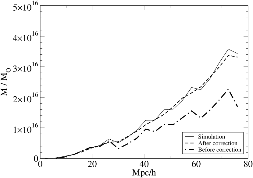
Figure 20: Magnitude limitation/Filling missing mass – This plot gives the measured amount of mass in a thin shell at different distances from the observer. The solid line gives the original mass distribution in the simulation, the dot-dashed line the mass distribution after mimicking incompleteness and the dashed line the recovered mass distribution after correction for incompleteness as described in Appendix C.

Appendix D Statistical bias in the slope estimation

The two methods that we used for slope estimation are known to be biased. A more precise treatment of this bias is beyond the scope of this paper. However we propose here to check the order of magnitude of the systematic effect of the statistical analysis itself. To achieve this we produced a set of randomly generated “velocities” $v$ and their “reconstructed velocities” $v_{\text{R}}$ counterpart. The probability for a point $(v,v_{\text{R}})$ to have a velocity $v$ is given by

$$P_{v}(v)=\frac{1}{\sqrt{2\pi}\sigma_{v}}\text{e}^{-v^{2}/(2\sigma_{v}^{2})}\text{,}$$ (52)

with $\sigma_{v}=300$ km s^-1typically. The probability for it to have a reconstructed velocity $v_{R}$ is given by the same probability law. We now compute the error $e$ between $v_{R}$ and $v$, which must be distributed according to the Lorentzian form

$$P_{\text{DE}}(e)=\frac{1}{\pi B}\frac{1}{1+\left(\frac{e}{B}\right)^{2}}\text{,}$$ (53)

with $B=86$ km s^-1. The error $e$ is related to $v$ and $v_{\text{R}}$ by

$$e=\alpha_{*}v-\beta_{*}v_{\text{R}}\text{.}$$ (54)

For the rest of the appendix we take $\alpha_{*}=\beta_{*}=1/\sqrt{2}$. The probability of keeping a point $(v,v_{R})$ with an error $e$ is given by, integrating $P_{\text{DE}}(e^{\prime})$ between $-e$ and $+e$,

$$P_{\text{keep}}(e)=\frac{2}{\pi}\tan^{-1}\left(\frac{e}{B}\right)$$ (55)

We represented in Fig. 21 a scatter plot of 10,000 points generated using this procedure. As one can see, it does look like a real scatter plot of a redshift reconstruction.

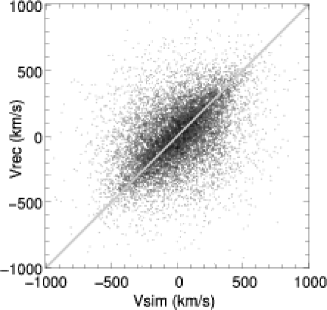
Figure 21: Statistical bias – Scatter plot of 10,000 randomly generated points following the approximated probability laws found between reconstructed velocities and simulated velocities.

Conducting a 1.5$\sigma$ analysis on this set of points, we find a slope $\beta_{*}/\alpha_{*}=1.0\pm 0.20$. In our case, this would give $\Omega_{\text{m}}=0.30\pm 0.10$. Estimating the slope using the maximum likelihood approach gives, with $\sigma_{v}=+\infty$, $\beta_{*}/\alpha_{*}=0.81\pm 0.01$ ($\Omega_{\text{m}}=0.20\pm 0.02$) and with $\sigma_{v}=300$ km s^-1, $\beta_{*}/\alpha_{*}=1.074\pm 0.012$ ($\Omega_{\text{m}}=0.34\pm 0.02$). Putting $B=40$ km s^-1, both for generated data and likelihood function, as for real space reconstructions, reduces the error and gives $\Omega_{\text{m}}=0.31\pm 0.02$, thus highlighting the importance of the reconstruction noise for a good estimation of $\Omega_{\text{m}}$.

Consequently, though one must rely on the likelihood analysis, it may be strongly biased by the structure of reconstruction errors mixed with the non-uniform distribution of observables. We tried to make a good approximate model of the errors, though it seems to quite depends on the value of $\sigma_{v}$. Whenever possible, of course, one must crosscheck the result of the likelihood by a visual inspection of the scatter plot.

References

- Peebles (1989) Peebles P. J. E., 1989, ApJL, 344, L53
- Tully (2005) Tully R. B., 2005, ApJ, 618, 214
- Kaiser (1987) Kaiser N., 1987, MNRAS, 227, 1
- Peebles (1980) Peebles P. J. E., 1980, The large-scale structure of the universe. Research supported by the National Science Foundation. Princeton, N.J., Princeton University Press, 1980. 435 p.
- Bertsekas (1979) Bertsekas D. P., 1979, A Distributed Algorithm for the Assignment Problem. MIT Press, Cambridge, MA
- Strauss & Willick (1995) Strauss M. A., Willick J. A., 1995, Phys. Rept., 261, 271
- Huchra et al. (1992) Huchra J. P., Geller M. J., Clemens C. M., Tokarz S. P., Michel A., 1992, Bulletin d’Information du Centre de Donnees Stellaires, 41, 31
- Mohayaee et al. (2006) Mohayaee R., Mathis H., Colombi S., Silk J., 2006, MNRAS, 365, 939
- Couchman et al. (1995) Couchman H. M. P., Thomas P. A., Pearce F. R., 1995, ApJ, 452, 797
- Tully (1987) Tully R. B., 1987, ApJ, 321, 280
- Colombi et al. (2007) Colombi S., Chodorowski M. J., Teyssier R., 2007, MNRAS, 375, 348
- Bardeen et al. (1986) Bardeen J. M., Bond J. R., Kaiser N., Szalay A. S., 1986, ApJ, 304, 15
- Mohayaee & Tully (2005) Mohayaee R., Tully R. B., 2005, ApJL, 635, L113
- Regos & Szalay (1989) Regos E., Szalay A. S., 1989, ApJ, 345, 627
- Efstathiou et al. (1988) Efstathiou G., Frenk C. S., White S. D. M., Davis M., 1988, MNRAS, 235, 715
- Bouchet et al. (1995) Bouchet F. R., Colombi S., Hivon E., Juszkiewicz R., 1995, A&A, 296, 575
- Sheth & Tormen (2002) Sheth R. K., Tormen G., 2002, MNRAS, 329, 61
- Bertschinger & Dekel (1989) Bertschinger E., Dekel A., 1989, ApJL, 336, L5
- Shaya et al. (1995) Shaya E. J., Peebles P. J. E., Tully R. B., 1995, ApJ, 454, 15
- Fontanot et al. (2003) Fontanot F., Monaco P., Borgani S., 2003, MNRAS, 341, 692
- Valentine et al. (2000) Valentine H., Saunders W., Taylor A., 2000, MNRAS, 319, L13
- Zandivarez et al. (2006) Zandivarez A., Martínez H. J., Merchán M. E., 2006, ApJ, 650, 137
- Branchini et al. (2002) Branchini E., Eldar A., Nusser A., 2002, MNRAS, 335, 53
- Croft & Gaztanaga (1997) Croft R. A. C., Gaztanaga E., 1997, MNRAS, 285, 793
- Lahav et al. (1994) Lahav O., Fisher K. B., Hoffman Y., Scharf C. A., Zaroubi S., 1994, ApJL, 423, L93+
- Marinoni & Hudson (2002) Marinoni C., Hudson M. J., 2002, ApJ, 569, 101
- Tully et al. (2007) Tully R. B., Shaya E. J., Karachentsev I. D., Courtois H., Kocevski D. D., Rizzi L., Peel A., 2007, ArXiv e-prints, 705
- Eisenstein et al. (2006) Eisenstein D. J., Seo H.-j., Sirko E., Spergel D., 2006, ArXiv Astrophysics e-prints
- Falco et al. (1999) Falco E. E., Kurtz M. J., Geller M. J., Huchra J. P., Peters J., Berlind P., Mink D. J., Tokarz S. P., Elwell B., 1999, PASP, 111, 438
- Phelps et al. (2006) Phelps S. D., Desjacques V., Nusser A., Shaya E. J., 2006, MNRAS, 370, 1361
- Tully & Pierce (2000) Tully R. B., Pierce M. J., 2000, ApJ, 533, 744
- da Costa et al. (1988) da Costa L. N., Pellegrini P. S., Sargent W. L. W., Tonry J., Davis M., Meiksin A., Latham D. W., Menzies J. W., Coulson I. A., 1988, ApJ, 327, 544
- Brenier et al. (2003) Brenier Y., Frisch U., Hénon M., Loeper G., Matarrese S., Mohayaee R., Sobolevskiĭ A., 2003, MNRAS, 346, 501
- Pizagno et al. (2006) Pizagno J., Prada F., Weinberg D. H., Rix H.-W., Pogge R. W., Grebel E. K., Harbeck D., Blanton M., Brinkmann J., Gunn J. E., 2006, ArXiv Astrophysics e-prints
- Erdoğdu et al. (2006) Erdoğdu P., Lahav O., Huchra J. P., Colless M., Cutri R. M., Falco E., George T., Jarrett T., Jones D. H., Macri L. M., Mader J., Martimbeau N., Pahre M. A., Parker Q. A., Rassat A., Saunders W., 2006, MNRAS, 373, 45
- Spergel et al. (2006) Spergel D. N., Bean R., Dore’ O., Nolta M. R., Bennett C. L., Hinshaw G., Jarosik N., Komatsu E., Page L., Peiris H. V., Verde L., Barnes C., Halpern M., Hill R. S., Kogut A., Limon M., Meyer S. S., Odegard N., Tucker G. S., Weiland J. L., Wollack E., Wright E. L., 2006, ArXiv Astrophysics e-prints
- Bennett et al. (2003) Bennett C. L., Halpern M., Hinshaw G., Jarosik N., Kogut A., Limon M., Meyer S. S., Page L., Spergel D. N., Tucker G. S., Wollack E., Wright E. L., Barnes C., Greason M. R., Hill R. S., Komatsu E., Nolta M. R., Odegard N., Peiris H. V., Verde L., Weiland J. L., 2003, ApJS, 148, 1
- Tegmark et al. (2006) Tegmark M. et al., 2006, Phys. Rev. D, 74, 123507