UCB-PTH-07/12
LBNL-62798
CALT-68-2654
UT-07-19
Statistical Understanding of Quark and Lepton Masses
in Gaussian Landscapes
Lawrence J. Hall,a Michael P. Salemb and Taizan Wataric
a Department of Physics and Lawrence Berkeley National
Laboratory,
University of California, Berkeley, CA 94720, USA
b California Institute of Technology, Pasadena, CA 91125, USA
c Department of Physics, the University of Tokyo, Tokyo, 113-0033, Japan
| – | |||
|---|---|---|---|
| (90% CL) | |||
| – | – (90% CL) | ||
| (95% CL) | |||
| eV2 | eV | ||
| eV2 | eV | ||
| – |
1 Introduction
The Standard Model111We everywhere refer to the “Standard Model” as the theory including the dimension-five operators of (1). describes all laboratory data with 28 free parameters. Of these, 22 arise from the Yukawa matrices and the coupling matrix that appear in the flavor interactions
| (1) |
where () are the left (right) handed quark and lepton fields. Of these 22 flavor parameters, 17 are measured, with varying levels of accuracy. The remaining five parameters are all in the neutrino sector and two of these have upper limits. Given several decades of continued progress on improving the accuracy of the experimental measurements, the most striking fact is that there is nothing approaching a standard theory of the origin of these parameters. Not only are we ignorant about the overall picture of flavor, we do not have a convincing explanation for the value of any of the 17 measured parameters.
A complete theory of flavor would provide answers to three very different questions:
-
•
What is the origin of the fermion quantum numbers and why are there three generations?
-
•
What determines the qualitative pattern of the quark and lepton mass matrices? For example, why do the charged fermion masses and mixings have a hierarchical pattern, while in the neutrino sector there are large mixing angles?
-
•
What determines the precise values of the 22 flavor parameters?
The couplings and are symmetry breaking parameters of the flavor symmetry group , where one factor acts on each of . The dominant approach to constructing theories of flavor is to use symmetries to reduce the number of free parameters, . An underlying flavor group and a more unified gauge symmetry both limit , leading to precise predictions if , the number of observables. A hierarchy of symmetry breaking scales can lead to small dimensionless parameters that explain qualitative features of the mass matrices [2], and there are many realizations with both Abelian and non-Abelian. Still, it is striking that the progress along these lines is limited, even as more precise data have become available. Perhaps this is a sign that a completely new approach is needed.
The cosmological dark energy [3] apparently has little to do with flavor. However, it may be the first evidence for a huge landscape of vacua, with the observed value of the cosmological constant resulting from environmental selection for large scale structure [4]. If we take string theory to be a theory of a landscape rather than a theory of a single vacuum, then what are the implications for flavor? The enormous number of vacua, required for a sufficiently fine scan of the cosmological constant, results from the large number of ways background fluxes can be arranged on non-trivial compact manifolds of extra spatial dimensions [5]. The cosmological constant, however, is not the only parameter that scans over such a landscape. The Yukawa couplings may also vary from one universe to another.
In any landscape of vacua, the Yukawa couplings have a relevant dependence on parameters, where of the parameters scan and of them are fixed. If then data can determine the subset of vacua in which we happen to live and predictions can be made. A certain simple model with a single extra dimension has , giving a single prediction [6]. If , however, then no such precise predictions are possible. Some flavor parameters—such as the electron, up and down masses—may be determined by environmental effects [7]. The top mass may also be determined along this line [8], while selecting for leptogenesis may be a key to understanding some parameters in the lepton sector. However, most of the flavor parameters do not seem to be strongly selected. Therefore it could be that most flavor parameters have values that simply reflect some underlying probability distribution over an enormous number of solutions to the fundamental theory. The precise value of any such observable is accidental and not fundamental, since any other nearby value would be just as probable. Although it may be unappealing that there is nothing fundamental or beautiful relating the flavor parameters in our universe, so far this possibility cannot be dismissed, especially given that no such relations have been found.
The large mixing angles observed in atmospheric and solar neutrino oscillations inspired the idea that the relevant Yukawa couplings of the neutrino sector are governed by randomness rather than by flavor symmetries [9]. By introducing a simple probability distribution for the elements in the Dirac and Majorana neutrino mass matrices, probability distributions for the neutrino observables were generated and found to agree well with data. However, a complete landscape approach to the theory of flavor must explain many other things; there are rich structures among the observed flavor parameters. Reference [10] took a bold step in this direction, studying masses and mixings in both the quark and lepton sectors by introducing a simple probability distribution for the Yukawa couplings. We begin in section 2 by analyzing the toy landscape introduced in [10]. While the main purpose of this section is to clarify how hierarchy among quark masses is generated in this model and to point out its limitations, we also introduce an approximate analytical study of the probability distribution of flavor observables. This turns out to be a useful warm-up exercise for the subsequent sections.
Ideally, a statistical approach to the theory of flavor would be both phenomenologically successful and theoretically well-motivated. However to determine the probability distributions for flavor parameters from a purely top-down calculation is not an easy task; meanwhile the number of observables is limited, and such low-energy information does not constrain the underlying probability distributions in a purely bottom-up approach. We consider as a practical strategy to use string theory as a guide in deducing the form of the probability distributions, while using known experimental constraints to try to find a phenomenologically successful model within this restricted set of possibilities. In a given compactification of string theory, the Yukawa couplings are determined by an overlap integration over the extra spatial dimensions. Scanning moduli parameters of the gauge field configuration on the extra dimensions corresponds to scanning zero-mode wavefunctions, and hence this corresponds to scanning Yukawa couplings. If the wavefunctions of the quarks, leptons, and the Higgs are peaked at different locations, then the overlap integral can lead to small Yukawa matrix elements. Hence localization in extra dimensions is an alternative to symmetries for generating fermion mass hierarchies [11].
In sections 3 through 6 we introduce simple “Gaussian landscapes” and study the resulting distributions for quark and lepton masses and mixings.222A brief summary of some of the major results of this work can be found in [12]. These landscapes have features expected from certain string landscapes, for which they can be viewed as simplified or toy models. The key feature of a Gaussian landscape is that all quark, lepton and Higgs fields have zero-mode wavefunctions with Gaussian profiles in the extra dimensions, and that the centers of these profiles all scan independently with flat probability distributions over the volume of the extra dimensions. For simplicity, the number of free parameters used to describe the geometry of the extra dimensions and the widths of the Gaussian profiles is kept to a minimum. We find the observed quark and lepton masses and mixings can be typical in such simple landscapes.
In section 3 we introduce a Gaussian landscape for quarks on a circle , with all Gaussian profiles having the same width. Numerical probability distributions for the nine CP-conserving flavor observables are provided, and a qualitative semi-analytic description of these distributions is derived. The results are compared with those that result from introducing approximate flavor symmetries, with some similarities and some differences emerging. Finally, the effects of possible environmental selection on the top quark mass is studied. The large number of flavor parameters in the Standard Model allows for a reasonably significant evaluation of goodness-of-fit between a Gaussian landscape and the observed flavor structure. This is described in section 4, with the Gaussian landscape used for illustration. The effects on the quark sector from adding more dimensions to the Gaussian landscape are examined in section 5, together with a preliminary study of the effects of geometry.
In section 6 the Gaussian landscape is extended to include the lepton sector. Motivated by the expectation of supersymmetry in the higher dimensional theory, Yukawa couplings for both Dirac and Majorana neutrino masses are introduced in the Gaussian landscape, with light neutrinos resulting from the usual seesaw mechanism in four dimensions. Larger mixing angles in the lepton sector might arise from assigning the appropriate fermions larger Gaussian widths, but these are found to largely cancel between charged and neutral sectors. However, this cancellation is prevented by introducing CP-violating phases in the Gaussian profiles. This suggests a connection in Gaussian landscapes between large CP violation and large leptonic mixing angles. In addition to providing numerical distributions for the observed lepton flavor parameters, probability distributions are predicted for the leptonic mixing angle , the CP phase in neutrino oscillations, and the Majorana mass relevant for neutrinoless double beta decay, illustrating how these toy models for the string landscape can connect to future experimental data. Finally, the extent to which these Gaussian landscapes arise from unified supersymmetric field theories in higher dimensions is examined in section 7. Such theories have huge symmetries—ultimately all entries of the Yukawa matrices arise from a unified supersymmetric gauge coupling—so that the complicated pattern of observed masses and mixings can arise from a very simple mechanism: the scanning of the centers of the Gaussian profiles.
2 Prelude: Hierarchy without Flavor Symmetry
In previous work it has been suggested that the components of the Yukawa matrices and the coupling matrix are selected randomly and independently of each other [9, 10]. For example, in Neutrino Anarchy [9] one finds that the large mixing angles underlying neutrino oscillation are typical of the lepton interactions that arise when each element of the matrices and is independently selected from the simple probability distributions
| (2) |
or from distributions such as
| (3) |
where and are of order unity (for more details see [9, 13]). Such an absolute anarchy of lepton couplings tends to result in comparable mass eigenvalues. On the other hand, [10] introduced a power-law probability distribution for the Yukawa matrix elements, for and otherwise. By assuming and choosing appropriately, quark Yukawa matrices with each matrix element following such a distribution can roughly accommodate the hierarchical pattern of quark mass eigenvalues [10]. According to [10], provides the best fit to the quark sector.
In this paper we propose a significant modification to these ideas. However as a prelude to discussing our proposal it is worthwhile to first study the model of [10] in greater detail. To simplify the analysis we specialize to the particular case , such that
| (4) |
Henceforth we refer to this distribution as a scale-invariant distribution. In this section we also restrict attention to the quark sector. Note that CP-violating phases are not introduced in this landscape because all of the matrix elements are real-valued. A pair of Yukawa matrices and is generated by choosing each of the 18 matrix elements randomly according to the distribution (4). The Yukawa matrices are then diagonalized using separate left- and right-handed unitary transformations, and the quark masses and mixings are calculated from the eigenvalues of the diagonalized Yukawa matrices and the resulting CKM matrix. The above process is then repeated to generate an ensemble of these nine observables.
2.1 The Distribution of Mass Eigenvalues
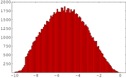
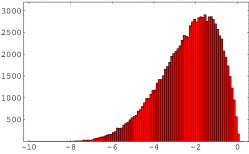
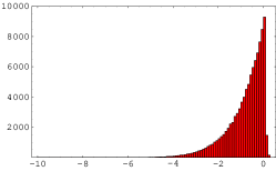
We first study the distributions of the quark masses. Since the up- and down-type Yukawa matrices are generated independently of each other and in exactly the same way, the distributions of masses for these sectors are exactly the same. Thus we only need to study one of the two sectors. Results of a numerical study are shown in Figure 1, where we have chosen .
 |
 |
 |
With some approximations we can understand the shapes of these distributions. Let denote the largest element of the matrix . Meanwhile, the largest element of the sub-matrix of that excludes is denoted . For example, in the matrix
| (5) |
is the largest among the nine entries and the largest in the upper right sub-matrix. Given this characterization, the probability distribution for the variables and is
| (6) | |||||
where is the step function. The factor of 36 comes from the nine possible locations for times the four possible locations for . In addition we have introduced the notation
| (7) |
The largest mass eigenvalue of (5) is approximately ; this approximation is poor if one of , , and is almost as large , but this is unlikely if is large. We call this largest eigenvalue and define analogously to . The probability distribution of is therefore approximated by integrating out from (6) all the variables except :
| (8) |
Meanwhile, we approximate the middle eigenvalue by and the smallest eigenvalue by . This approximation is poor when the seesaw contributions and are larger than and , respectively. Thus we do not expect this approximation to be reliable for small values of and . Nevertheless, integrating out all of other variables we find
| (9) | |||||
| (10) |
 |
 |
 |
Remarkably, they capture the gross features of the numerical results in Figure 1. Therefore we use these distributions to examine the qualitative aspects of the mass distributions that follow from the landscape (4).
The average and the standard deviation of the three Yukawa eigenvalues (both on a logarithmic scale) can be calculated from the distributions (8–10):
| (11) | |||||
| (12) | |||||
| (13) |
The three eigenvalues are on average well-separated and they overlap with neighboring eigenvalues only slightly at one standard deviation. Even this slight overlap between the distributions is misleading. Recall that by definition for any particular set of Yukawa matrices we have . Thus the combined distribution for the eigenvalues is not a naive product of (8–10) but is given by integrating the other six variables out of (6). This gives
| (14) |
Thus it happens that in the subset of cases where is small, the distribution of is pushed to even smaller values. Hence the three eigenvalues tend to be well-separated even in the logarithmic scale, and only rarely are adjacent eigenvalues comparable. Note that none of this depends on the choice of and . In short, hierarchical structure (Yukawa eigenvalues well-separated in logarithmic scale) is generated statistically in a landscape where each matrix element independently follows the scale-invariant distribution (4). Whether the hierarchy is large or small is determined by whether is large or small.
2.2 Pairing Structure in Electroweak Interactions
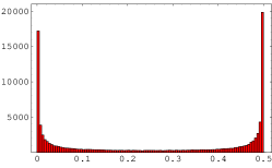
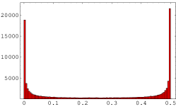
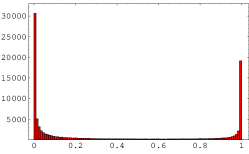
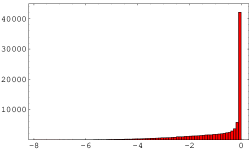
Let us now study the mixing angles. Figure 3 shows the distributions of mixing angles in the quark sector that result from a numerical simulation where each element of both the up-type and down-type Yukawa matrices is assumed to follow the distribution (4) independently.333Using (8–10) we find these distribution functions to be given by the approximate analytic form: (15) (16)
 |
 |
 |
 |
 |
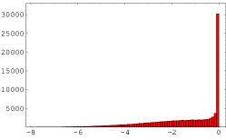 |
The probability distribution functions of the mixing angles are shown against the axes of , and because the invariant measure444The importance of the invariant measure is emphasized in [13]. of SO(3) mixing matrices is . Since in this model the Yukawa couplings are all real- and positive-valued, the CKM quark mixing matrices are SO(3) matrices.
The prominent feature of these distributions is the twin peaks at and for all three mixing angles. This feature is straightforward to understand. Suppose that the randomly generated Yukawa matrices are of the form
| (17) |
where the ’s are assumed to be less than or , and the ’s less than or . Ignoring the seesaw contributions to eigenvalues, i.e. when and , we find that the three left-handed quark doublets () are approximately
| (18) |
where , and stand for left-handed components of the heaviest, middle and lightest mass eigenstates of up-type quarks. The down-type mass eigenstates , and are defined similarly. The CKM matrix for the up-type and down-type Yukawa matrices (17) is roughly
| (19) |
corresponding to and . This explains one of the combinations of peaks in Figure 3. When the are found in different entries of the Yukawa matrices, other peak combinations are obtained. Continuous distributions connecting to originate from the seesaw contributions that we have ignored. Thus the distributions become more and more localized around the peaks as is increased and seesaw contributions become less important. Therefore the small mixing angles of the observed CKM matrix are not atypical of distributions with large values of .
How then do we interpret the peaks at ? The flavor structure of the quark sector of the Standard Model is characterized by three general features. On the one hand, the quark masses have a hierarchical structure, and this is successfully reproduced. In addition, the -boson current approximately connects three distinct pairs of quarks—we refer to this as “pairing structure,” and it is also found in this landscape. Finally, the -boson current connects pairs such that the lightest up-type quark is approximately paired with the lightest down-type quark, the middle up-type quark is approximately paired with the middle down-type, etc. We refer to this as the “generation structure” of the Standard Model. Mixing angles near maximally violate this generation structure; for example the set of angles and of (19) corresponds to the quark pairings in (18). There are combinations in forming three pairs, only one of which has what we call the generation structure.555 When , and result in the same quark combinations. Likewise, and are the same. Therefore there are only physically different combinations, even though there are different ways to pick three peaks from Figure 3.
2.3 Problems
Is the existence of mixing angle peaks about really a problem? The landscape that we have discussed so far may reproduce the generation structure of mass eigenstates in the -boson current (when ), but more often it does not. Although it might be argued that this is just a coincidence problem, it is still difficult to accept that the generation structure of flavor is not revealing something important about the underlying theory. It is also tempting to try read something deeper from the observed hierarchy between and the Cabibbo angle . In this landscape this hierarchy is just a random statistical fluctuation (c.f. Figures 2 and 3), and it does not appear this shortcoming can be overcome by a more ideal choice of (c.f. Figure 1).
An even bigger problem is to understand how the probability distribution (4) arises or what is the correct distribution to replace it. That is, although the phenomenology of the landscape that we have considered may be deemed acceptable, we do not have a solid theoretical ground upon which to base it.666Such an attempt is made in [14]. However, we consider that correlation among Yukawa couplings and the number of extra dimensions are crucial ingredients in understanding flavor physics, and these are missing in [14]. The intersecting D6–D6 system mentioned in [14] is dual to a -fibered compactification of Heterotic string theory and is simulated by the Gaussian landscape models of this article. Although [14] guesses that the scale invariant (or nearly scale invariant power-law) distribution might arise from the intersecting D-brane systems, we conclude otherwise. Specifically, we find that the scale-invariant distribution (4) is derived from the Gaussian landscape model, but not a model. We also find that correlation among various elements of the Yukawa matrices is crucial to understanding flavor structure and the origin of generations. It is also obscure how the phenomenology of a lepton sector with large mixing angles and that of quark sector with small mixing angles can be accommodated within a single theoretical framework. In the remaining sections of this paper we analyze some landscape models that successfully reproduce the phenomenology of hierarchy, pairing, and generation structure, while making progress on each of the four problems described above.
3 A Gaussian Landscape for Quarks in One Extra Dimension
The landscape discussed in section 2 assumes that all 18 elements of and are scanned independently. Yet without any correlation between these two Yukawa matrices, generation structure will never be obtained. For example, in order to ensure that the heaviest up-type quark is contained in the same SU(2)L doublet as the heaviest down-type quark , we require the following. When an (, ) element of the up-type Yukawa coupling is large, at least one of the three down-type Yukawa couplings () involving the same quark doublet should be large. A landscape of vacua must realize such a correlation between the up-type and down-type Yukawa matrices in order to explain the generation structure.
Perhaps one of the simplest ideas to introduce such a correlation is to introduce an extra dimension. If a large Yukawa coupling of is due to a substantial overlap of the wavefunctions of and , then the down-type Yukawa couplings involving the same tend to be larger because of the overlap of and . At the same time, for localized wavefunctions the overlap of some triplets of , and can be very small, and so there is hope to explain the hierarchically small Yukawa couplings necessary to account for light quarks.
In this section we present a simple toy landscape based on Gaussian wavefunctions spanning a circular extra dimension. Although a single extra dimension is introduced for simplicity, this model captures the essence of what one expects more generally from such “Gaussian landscapes” based on multiple extra-dimensional field theories. Through numerical simulation and an approximate analytical analysis, we find that the hierarchy, pairing, and generation structures of quarks is obtained statistically in this landscape. No flavor symmetry is needed.
3.1 Emergence of Scale-Invariant Distributions
We introduce a single extra dimension with the simplest geometry: . The wavefunctions for all of the quarks and the Higgs boson are assumed to be Gaussian with a common width , and centered at arbitrary points on :
| (20) |
Here is the coordinate of and is the cut-off scale of the effective field theory in dimensions. This wavefunction is normalized so that
| (21) |
where is the circumference of . The wavefunction (20) should be made periodic on , while maintaining the normalization in (21). Yet as long as the width of the Gaussian profile is parametrically smaller than the circumference , the wavefunction is almost Gaussian. One should examine whether Gaussian wavefunctions arise as solutions to equations of motion of field theories in extra dimensions, but we defer this theoretical study to section 7, and first study whether the assumption of Gaussian wavefunctions on extra dimensions leads to a successful explanation of the physics of quark and lepton masses and mixing angles.
We calculate the up-type and down-type Yukawa matrices with the overlap integrals
| (22) |
where is an overall constant.777We will see in section 7 that these interactions may originate from super Yang–Mills interactions on a higher dimensional spacetime, and then derives from the Yang–Mills coupling constant. Despite this origin, can be different in different sectors in effective descriptions such as those using just one extra dimension. For simplicity we set the constant to be the same for both the up and down sectors. , , and are wavefunctions of left-handed quark doublets (), right-handed up-quarks (), right-handed down-quarks () and of the Higgs boson, respectively, all of the Gaussian form (20).888In section 7 we study higher dimensional supersymmetric field theories, where at short distances the up-type and down-type Yukawa couplings involve different Higgs doublets, . Our results are independent of whether or not supersymmetry survives to the weak scale. If a supersymmetry survives compactification, we assume that the zero modes have the same localization. If no supersymmetry survives then we assume a single Higgs zero mode with a Gaussian profile. There is a “” factor between the up and down sectors that we have set to unity. With weak scale supersymmetry this factor arises from the ratio of Higgs vacuum expectation values, while with high scale supersymmetry breaking it arises from the composition of the light Higgs boson. The center coordinates of these wavefunctions are , , and , respectively. The matrices are real, so that CP is conserved in this toy landscape. Complex Gaussian wavefunctions will be studied in section 6, where the effects of phases on the distributions of quark masses and mixing angles is found to be small. We assume that the center coordinates , , and are scanned freely and independently from one another on . Because of the translational symmetry of , only the relative difference between these center coordinates affects observables. Thus the effective number of scanning parameters is . On the other hand, there are nine observables determined from the Yukawa matrices in the quark sector: six mass eigenvalues and three mixing angles. Thus the scanning parameters cover the space of observables and no precise prediction among the observables is available. However, since this Gaussian landscape covers the space of observables, our vacuum is unlikely to be missed in this ensemble.
The other model parameters, namely the width , circumference , cut-off scale , and coupling , are treated as fixed. This treatment is quite arbitrary; among the myriad of other possibilities are to scan some or all of these parameters, to allow the up-sector and the down-sector to have different values of , to choose different widths for different wavefunctions, etc. An extreme version of the landscape would allow everything to scan, leaving no fixed parameters to be input by hand. Our treatment—namely four fixed parameters—is equivalent to slicing a specific subset out of a possibly much larger landscape. This allows us to identify a phenomenologically successful subset of the landscape and at the same time more easily explore its properties. It is a separate question whether this subset is typical of the full landscape, or if it is highly weighted because of cosmological evolution and/or environmental selection. Indeed, it is not implausible that the distributions of these four fixed parameters could be sharply peaked in the full landscape, since some toy landscapes predict Gaussian distributions for some parameters and cosmological evolution can provide exponentially steep weight factors. We consider that practical progress can be made by dividing the full problem into simpler parts.
Note that out of these four fixed parameters there are only two independent combinations that affect the Yukawa matrices. First, only the three dimensionless combinations, , , and , are physical; the value of simply sets the scale for dimensionful parameters. Second, even as we change the “volume” of the extra dimension , the Yukawa couplings remain the same if the width parameter and the coupling are scaled so that the ratio and the effective coupling,
| (23) |
remain the same. Therefore the Yukawa couplings are effectively controlled by only these two parameters, and . (Note however that the volume does affect the low-energy value of Newton’s constant.)
The Yukawa couplings, given by the overlap integrals (22), can be expressed more explicitly in terms of the underlying parameters in a restricted region of the parameter space. Suppose that . Then the compactness of is not important in the calculation of the Yukawa couplings, as long as the center coordinates of quarks, (or ) and , are close to that of the Higgs boson (which, by translational invariance, we set as the origin of the coordinate ). For such a vacuum, the Yukawa couplings are given by
| (24) |
Let us compare this result to the form for the Yukawa couplings that results from approximate Abelian Flavor Symmetries (AFS). In the most general AFS scheme there is a small symmetry breaking factor associated with each quark field, , which leads to Yukawa matrix elements
| (25) |
where the and are all of order unity. A mass hierarchy among the generations is realized by imposing in the left, right, or both sectors. Models with fewer parameters can be constructed and then the symmetry breaking parameters are not all independent; consider for example a single Abelian symmetry with a symmetry breaking parameter that appears in different entries with different powers due to generation dependent charges. Generation charges (0,2,3) then give . No matter how the model is arranged, the mass hierarchy arises because the first generation feels much less flavor symmetry breaking than the third. Note that AFS theories are very flexible—any hierarchical pattern of fermion masses can be described by an appropriate AFS.
The result (24), which involves no flavor symmetry, has some similarities with the form (25). First notice that , , and can be both positive and negative and therefore the factor of (and ) in (24) is statistically neutral. Anticipating this statistical averaging, we cast (24) into the form of (25) with the identification
| (26) |
An important feature is that the AFS factor is shared by all elements of both the up-type and the down-type Yukawa couplings that involve the left-handed quark doublet . This introduces a correlation between the up-type and down-type Yukawa matrices.
We first study the probability distribution for a single entry in the Yukawa matrix, ignoring correlations with other entries. This allows us to determine the analogue of (4) for this Gaussian landscape.
 |
 |
 |
Here we do not have a distinction between the up-type and down-type Yukawa matrices because we assume that the center coordinates of both the and wavefunctions are distributed randomly over . The up-type Yukawa coupling in (24) is a function on the two-dimensional parameter space . The probability that the Yukawa coupling is larger than some value is proportional to the area of an ellipse,
| (27) |
When the signs of and are opposite, the overlap of the three wavefunctions is small and the Yukawa coupling becomes small. This is why the region of is short in the axis and long in the axis. Comparing the area (27) to the total area , we see the probability that is given by
| (28) |
and hence the distribution is flat:
| (29) |
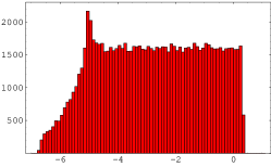
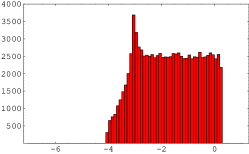
The distribution may cease to be flat as or approaches , where the parameter space ends, because we ignored the periodic boundary condition in the calculation that led to (24). Setting this point aside we see that the probability distribution of Yukawa couplings in this toy landscape is flat on the axis and has an approximate span of
| (30) |
arising from the inverse of the height of the distribution function (29). The overall hierarchy among Yukawa couplings is proportional to ; the narrower the wavefunctions become, the further the wavefunctions can be separated, and the smaller the Yukawa couplings can be. As seen from (24), the upper end of this scale-invariant distribution is roughly . Note that the scale-invariant distribution (4) was introduced almost by hand in [10] in order to account for the large hierarchy among Yukawa couplings. It is interesting that this distribution is a natural prediction of our simple Gaussian landscape.
We performed a numerical calculation to confirm the semi-analytical analysis above, taking account of the compactness of by making the wavefunction (20) periodic. The center coordinates of the quark wavefunctions were generated randomly times, and the Yukawa coupling was calculated through (22). This process was repeated for three different sets of the parameters: , and . The resulting distributions, shown in Figure 4, are all roughly scale-invariant (flat on a logarithmic scale), with heights proportional to , just as we expected from the semi-analytical discussion.
3.2 Quark-Sector Phenomenology of the Gaussian Landscape
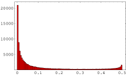
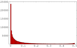
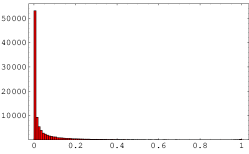
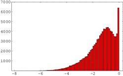
Let us now study the probability distributions of the mass eigenvalues and mixing angles. Figure 5 shows the result of a numerical simulation with .
 |
 |
 |
 |
 |
 |
 |
 |
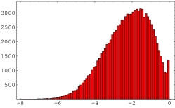 |
The distributions of Yukawa eigenvalues in Figure 5 are similar to those in Figure 1, but with narrower distributions of and with the distributions of shifted downward. The prominent difference between the mixing-angle distributions in Figure 5 and those in Figure 3 is the absence of the unwanted peaks at . Thus we find the generation structure of the quark sector follows from this Gaussian landscape; introducing correlations between the up-type and down-type Yukawa matrix elements works perfectly. Moreover, in contrast to Figure 3 the distribution of in Figure 5 has a clear peak at when displayed on a logarithmic scale.
The distributions of Yukawa eigenvalues and mixing angles in Figure 5 can be understood analytically if we allow ourselves to make an approximation.
 |
 |
 |
We have seen in section 3.1 that both the up-type and down-type Yukawa matrices have an AFS structure. Thus, we begin by determining the probability distribution of the AFS suppression factors in (26). The value of () is determined by the distance (, ) of the left-handed (right-handed) quark wavefunction from the Higgs boson wavefunction. Since the center coordinates are scanned randomly over the extra dimension , the probability measure is
| (31) |
The measure for the right-handed quarks is the same, and we only deal with the left-handed quarks hereafter. Converting the variable from to using (26), we find
| (32) |
where and we have defined .
The center coordinates of the three left-handed quark wavefunctions are chosen randomly, thus three AFS suppression factors follow (32) independently. The smallest of these corresponds to the suppression factor for the lightest quark, while the middle factor and largest factor correspond to the middle and the heaviest quarks. The distribution of is given by
| (33) |
where . Note that . The distributions of the individual AFS suppression factors are obtained by integrating (33) with respect to the other two variables:
| (34) |
These distribution functions are shown in Figure 6. Meanwhile, their averages are given by
| (35) |
In a sense, this Gaussian landscape predicts the ratio of the AFS charges for the three generations: 6:3:1. However this ratio only describes the statistical ensemble, and the distribution functions (34) contain more information.
The distributions of Yukawa eigenvalues follow from (34) with the approximation
| (36) |
Explicit expressions of the distribution functions derived in this way are found in the appendix, (197–205), and are plotted in Figure 6. From (197–205) we see that for small values of (these correspond to large eigenvalues), the distribution functions behave as , , and , which is confirmed in the numerical simulation in Figure 5. Note that the distribution of begins at around , and that of at around , contrary to the approximate analytic distribution functions (201,205), which begin at . This is probably due to the effects of diagonalizing the Yukawa matrices. As is familiar in quantum mechanics, two degenerate eigenvalues split even in the presence of the slightest perturbation. We later refer to this effect as the “diagonalization effect.”
We should also note that the AFS approximation (24, 26) breaks down for small values of Yukawa eigenvalues. The distributions based on the AFS approximation extend all the way down to , while the numerical results cover a logarithmic range closer to (30). Since , the analytically derived range of covers twice the logarithmic scale that we expect. This discrepancy arises from the compactness of the extra dimension. That is, what really matters in the exponent of (24) is
| (37) |
As the center coordinates and approach , non-zero choices of and may become just as important as in (24). Indeed, when integers and can be chosen so that the last term is negative. When the compactness of the extra dimension is taken into account, the full expression (37) cannot be larger than . This is why the distributions of Yukawa couplings and eigenvalues in Figure 4 and 5 span over in the numerical results. The AFS approximation breaks down because the coefficient is not statistically neutral when and are around .
Distribution functions of the mixing angles can also be obtained by pursuing the AFS approximation, along with the additional (crude) approximations:
| (38) | |||||
| (39) | |||||
| (40) |
Explicit expressions are found in (207–209) and are plotted in Figure 6. These approximate analytic distribution functions capture qualitative features of the numerical results. Note that the distribution function of becomes zero at because can be of order unity only when all three eigenvalues are almost degenerate in either the up- or down-sector, and the probability for this to occur is small. The averages of the mixing angles in a logarithm scale are ordered
| (41) |
both in the numerical simulation and in the analytic distributions; see (210). This is regarded as a consequence of the AFS charges in (35); indeed in (35) we have
| (42) |
Whether the assignments in (35) are observationally acceptable or not is debatable, and we will return to this issue in section 4. We discuss in section 5 how the “charge assignment” changes when the geometry is replaced by other geometries.
To summarize, we see that the qualitative expectations from an AFS-type mass matrix hold true in this landscape. In particular, the similarities between the landscape generated Yukawa couplings (24) and those of (25) allow us to understand Gaussian landscapes, at least to some degree, using intuition based on models of AFS. Of course, between these approaches the origin of small parameters is completely different: in the landscape they arise from small overlaps of wavefunctions well-separated in the extra dimension, whereas in AFS they arise from small symmetry breaking parameters. Let us now emphasize this distinction.
A crucial general feature of all AFS models is that the mass hierarchy between generations, , arises because there is a hierarchy in the amount of symmetry breaking coupled to these generations. This is true in the general Abelian case by the choice . In more restricted versions having , the hierarchy is imposed by a choice of charges . If the flavor symmetry is non-Abelian, then there is a hierarchy of symmetry breaking, for example the rank may be broken from to with strength . Thus AFS can in principle describe any flavor pattern, for example one heavy generation with Yukawas of order unity and two very light generations with Yukawas of order . The situation with this Gaussian landscape is very different. Each Yukawa coupling is a statistical quantity, with a probability distribution that is approximately scale invariant over a range determined by a single small parameter, . Relative to this range, the hierarchy of mass eigenvalues, including the typical inter-generational mass ratios and mixing angles, arises purely from statistics. Unlike with the AFS parameters , there is no sense in which the fundamental theory distinguishes among generations. Therefore unlike with AFS, this Gaussian landscape cannot accommodate one heavy generation and two very light generations of comparable mass. Within statistical uncertainties, the landscape determines the AFS charges.
3.3 Environmental Selection Effects
It is a formidable task to understand all of the environmental effects that would be associated with a landscape scanning over the flavor parameters of the Standard Model. Furthermore, without a specific theory for the landscape it is unclear whether certain qualitative features of the flavor sector arise due to environmental selection, due to systematic features of the landscape distributions, or due to accident. Consider these examples. In the Gaussian landscape of this section, tends to be smaller than . Therefore if is chosen so as to explain the hierarchy , then the relative lightness of the up and down quarks is explained. The value of required to reproduce the quark masses we measure may be selected dynamically within the fundamental theory or it may be selected due to environmental effects associated with having light up and down quarks. Likewise, the unexpected hierarchy may be due to the dynamical or accidental selection of different effective coupling constant ’s for the up and down sectors,999This hierarchy may also be due to weak-scale supersymmetry with a large ; however this requires that the wavefunctions for the up-type and down-type Higgs are located at the same position in the extra dimension. or environmental selection could favor a very large top mass as described in [8].
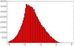
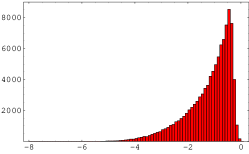
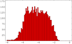
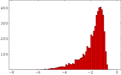
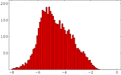
We now describe qualitative effects associated with one possibility for environmental selection, which is the selection of a large top mass to ensure the stability of our present Higgs phase [8]. Consider a simple cut on the top Yukawa:
| (43) |
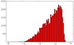
We emphasize that we impose this -cut to study qualitative effects; it is not intended to be precise. We first study the distributions of the quark Yukawa eigenvalues, which follow the distributions shown in Figure 7.
 |
 |
 |
 |
 |
 |
 |
 |
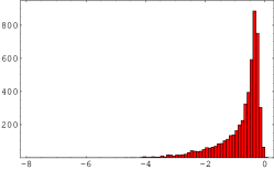 |
The three distributions in the first row correspond to Yukawa eigenvalues before the environmental cut is imposed. Since our landscape has not introduced any difference between the up- and down-type sectors, the three distributions are the same in both sectors. Imposing the -cut (43) reduces the sample to 5% of its original size. After the -cut is imposed, the eigenvalue distributions are modified into those displayed in the second and third rows of Figure 7. A notable effect of the -cut is that the distributions of the other Yukawa eigenvalues are dragged upward. This effect is more evident in the up-sector than in the down-sector, improving the fit of , , and .
One might consider that this improvement is not enough. Certainly the prediction is improved, but we find that the Standard Model value only moves from the 3rd to about the 6th percentile. Furthermore, the typical value of is large even without the -cut, and the distribution of is shifted upward after this cut is imposed. There are a number of ways to modify the Gaussian landscape of this section to alleviate this problem. Some of these have already been mentioned; others are presented in section 5, where we study how the geometry of the extra dimensions affects the distributions of observables in Gaussian landscapes.
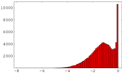
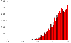
The effects of the -cut are also seen in the distributions of the mixing angles; see Figure 8.
 |
 |
 |
 |
 |
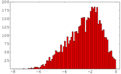 |
The probability that is reduced significantly, which is understandable because (and hence ) tends to be very close to in the sample passing the -cut, while and are rarely larger than . The distribution is reduced at small values as well, probably because the distributions of and are reduced at small values. Thus environmental selection on some flavor parameters modifies the distributions of other flavor parameters through a complicated chain of correlations.
3.4 Summary
We introduce a simple Gaussian landscape, based on a more microscopic description of the origin of flavor involving a single extra dimension, which predicts probability distributions for the CP-conserving quark sector flavor parameters. Using only two free parameters, and , this restrictive theory provides as good a fit to the flavor parameters as conventional theories of flavor based on flavor symmetries. This is especially so when the Gaussian landscape is augmented by environmental selection in favor of large top Yukawa coupling. This Gaussian landscape is characterized by the homogeneous scanning of the center coordinates of Gaussian wavefunctions in the extra dimension, which results in homogeneous scanning of Yukawa matrix elements on a logarithmic scale. The three eigenvalues of each Yukawa matrix then tend to be well separated from one another on the logarithmic scale. Thus, the hierarchical structure of quark mass eigenvalues is obtained. The wavefunctions of the three quark doublets and the Higgs boson are assumed to be quite localized in the extra dimension, and the overlap of these wavefunctions introduces correlation between the up-type and down-type Yukawa matrices. This is the essence behind (the microscopic explanation) for the generation structure of the quark sector, that is the phenomenon that the heaviest (middle and lightest) up-type quark is coupled to the heaviest (middle and lightest) down-type quark in the -boson current.
4 Goodness-of-fit Tests of Landscape Models
Before proceeding to generalize the Gaussian landscape, we here take an aside to discuss some possibilities for testing theories that assume a huge landscape of vacua. A landscape theory that contains the observed vacuum is not directly falsifiable in the convention sense, since we can only compare one value of any “variable” (the value in our universe) to its predicted distribution. On the other hand, with a statistical theoretical prediction we can at least calculate the probability to have measured a more atypical value for a landscape variable. If this probability is small, the landscape can be excluded at a certain confidence level. Indeed, the more numerous are the predictions of a landscape theory, the greater the possibility to exclude the theory. Consider for example quantum theory, where statistical theoretical predictions are well-tested using scattering experiments that count the event rates in a large number of bins/modes. The parameterization of the Standard Model is dominated by the 22 flavor parameters, 20 of which have either been measured or may be measured in the near future. Therefore it seems that the flavor structure of the Standard Model provides the best realm in which to test landscape theories.
In this section we study two statistical tests, the chi-square statistic and the p-value statistic, to illustrate how Gaussian landscapes may be excluded by experiment. As this section is intended to be only illustrative, we consider only the quark sector as described by the Gaussian landscape on (which in this section is referred to as the model) and we do not consider any weight factors that may arise due to cosmological evolution or environmental selection effects. The existence of correlations among the distributions of flavor parameters in Gaussian landscapes allows for a rich statistical analysis, and the discussion below only scratches the surface.
4.1 The Chi-Square Statistic
Our first example is to use the so-called chi-square statistic as a measure of goodness-of-fit between the observed flavor parameters and their hypothetical landscape distributions. The CP-conserving flavor parameters in the quark sector consist of the nine variables:
| (44) |
with the logarithm acting on every element of the list. The CKM phase is not included in this list because the model we consider here is CP-conserving. The chi-square statistic is
| (45) |
where hats denote the measured value of a parameter. The values listed in Table 1 are used for . Brackets denote the landscape average, and the co-variance matrix is given by
| (46) |
The chi-square statistic is invariant under any linear transformation among the variables .
The correlation among the parameters in (44) cannot be ignored. Specifically, for the three mass eigenvalues in the up sector, the correlation matrix, , is given by
| (47) |
Note that the off-diagonal terms are not negligible compared to the diagonal terms. The positive correlations are as expected from the combined probability distribution (33) of the AFS suppression factors . Meanwhile, the correlation between the up and down sector mass eigenvalues, , is given by
| (48) |
This is also sizable and positive, confirming that the mass eigenvalues in the down sector are dragged upward under the -cut. The mixing angles are also correlated with mass hierarchy; the correlation matrix between and is given by
| (49) |
where now and . We see that larger mass hierarchies are correlated with smaller mixing angles.
The covariance matrix determines the principal axes , with the covariance matrix being diagonal when the basis is changed to . Since is diagonal the observables are independent at least up to second order. If the distributions of the ’s were completely independent, and Gaussian, then the quantity would follow the chi-square distribution for random measurements of . This distribution has probability density
| (50) |
where is the number of independent Gaussian random variables entering (45). This distribution has a mean of and a standard deviation of . Thus the prediction is very sharp when a large number of observables are predicted by the landscape. Note that too large a value of indicates that the observed flavor parameters are atypical of what is expected from the landscape distributions, while too small a value of indicates that the correct underlying theory has less randomness than is exhibited by the landscape in question. Therefore, even though we can measure only one value for each observable, and hence measure only one value of , the chi-square statistic can still be a powerful tool in testing landscape theories.
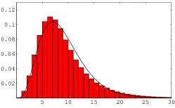
Our model predicts distributions for nine flavor parameters in the quark sector, but it contains free parameters ( and ) that can be fixed by hand and tuned101010In fact the free parameters and have not been fully exploited, since we have not performed a maximum likelihood analysis to determine the values that minimize in (45). However, the parameter values we use have been chosen to qualitatively fit our expectations for the measured values of . to fit two out of nine of the ’s, rendering two terms in to vanish. Thus we have independent degrees of freedom. Therefore if the distributions describing the were Gaussian, we would expect . In fact the model does not predict Gaussian distributions for any of the flavor parameters.
 |
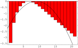 |
However, Figure 9 shows that the distribution of (45) using data generated by the model looks quite similar to the corresponding chi-square distribution, which has . Furthermore, the central limit theorem guarantees that as is increased the distribution of approaches a normal distribution with a mean and a variance that grows in proportion to . can be as large as 20 for the observable flavor parameters of the Standard Model, assuming a landscape with at least 20 scanning parameters.
We calculate the chi-square statistic for the nine CP-conserving quark-sector flavor parameters using the model to calculate and , and using Table 1 for . This gives , which agrees very well with the prediction . That the obtained value is neither too large nor too small indicates that the observed flavor parameters are typical and that they exhibit the expected level of statistical fluctuation in this landscape. The same analysis can be carried out for the model after a hypothetical environmental weight factor favoring a large top mass has been imposed. Using only model data that pass the -cut (43), we find , which also agrees well with the prediction. Imposing the -cut increases the value of , but one should keep in mind that the parameters and were chosen to fit the observed flavor parameters before imposing the -cut, without respect for the ensemble that passes the -cut.
4.2 The P-Value Statistic
The chi-square statistic has a disadvantage as well. Although the central limit theorem guarantees that for large that the distribution of approaches a normal distribution, regardless of most of the details of the actual distributions of the , is not more than 20 for the application to flavor parameters. Moreover, some of distributions of the flavor observables have sharp cut-offs, such that the probability to obtain a large value of may be much smaller than what is expected from a normal distribution with a mean and a variance . The chi-square statistic does not completely account for such a situation.
On the other hand, the p-value statistic is capable of handling non-Gaussian distribution functions. The p-value of a single flavor parameter is simply the fraction of the distribution that is more atypical than the measured value . Specifically, we may consider the p-value to be the fraction of the distribution that is farther from the median than is . If we approximate the probability density as continuous with profile , then the p-value is
| (51) |
Note that like , is a random variable for every independent measurement . However, whereas is distributed according to the chi-square distribution, is distributed uniformly between zero and one. The p-value is also the probability that the Kolmogorov–Smirnov statistic (the value of the function) of one sampling of the variable could have been larger than what is calculated from . Hence a measurement giving p-value excludes the corresponding theory at a confidence level of max%.111111P-values very near zero indicate that the measured values are collectively atypical of their predicted distributions; p-values very near unity indicate that the measured values do not exhibit the randomness expected from the predicted distributions.
Reference [15] used the p-value statistic to test the hypothesis of Neutrino Anarchy. There, the probability distribution of the lepton sector flavor parameters is factorized into those of mass eigenvalues, of each individual mixing angle, and of the CP phase [15]. Then the p-value statistic can be applied separately to each of the three mixing angles. In the case where the statistical variables are independent of each other, represents the fraction of the distribution of for which each element is more atypical than the measured value . The probability that could have been smaller than is given by (e.g. [15])
| (52) |
Here is simply a summation index used to simplify the last expression, and is the number of degrees of freedom in . For a random measurement of a set of independent variables , the p-value calculated through (52) is distributed uniformly from zero to one. Thus a random measurement giving p-value can exclude a landscape theory with a confidence level max%. If we treat the nine CP-conserving flavor observables in the quark sector as if they were independent, then the data and the hypothetical distributions of the model can be used to calculate the p-value through (52). Here, is used in (52) because the values of and can be tuned to bring two of the to be the same as their medians. We find , suggesting a good fit with observation.
In fact, however, the statistical variables are not independent. To the best of our knowledge, there is no standard definition of the p-value statistic for correlated multi-variable distributions. One possibility to account for correlation is to calculate by actually counting the fraction of randomly generated parameter sets that have each more atypical than that of the measured set . This is as opposed to using , which gives this fraction in the absence of correlations. In a sample of data sets generated using the numerical simulation of the model, we find 52 such sets, giving and hence . The uncertainty is obtained by assuming the variance in counting atypical data points is of the order of . Yet another attempt at a “p-value like” measure of the goodness-of-fit may be to judge atypicality by using in (51) the distributions of the principal axes , their measured values , and their medians —as opposed to using , , and —since the statistical variables do not have correlations, at least up to second order. The fraction of more atypical than the measured set can be calculated using ; using (52) we find this gives . If there were truly no correlations among the this would give the same result as calculating by actually counting the fraction of randomly generated parameter sets that have each more atypical than that of the measured set . However, in our ensemble of data sets we find just one for which each element is more atypical than its corresponding measured value, giving .
5 Geometry Dependence
In section 3 we introduced and analyzed a Gaussian landscape based on a single extra dimension, and found that it could provide the hierarchy, pairing, and generation structures of the observed quark sector. However, the number and geometry of extra dimensions need not correspond to the Gaussian landscape. Therefore, we initiate a study into how the compactification geometry of extra dimensions affects the probability distributions of observables. We find that the qualitative results of section 3 can be achieved by Gaussian landscapes in other geometries of extra dimensions and that the distribution functions of flavor observables are largely insensitive to the details of these geometries. However, the behavior of the distribution functions of mass eigenvalues at large values is affected by the number of extra dimensions. In section 7, we argue that the geometries used in Gaussian landscapes are related to base manifolds of torus-fibered geometries used in the compactification of string theory.
5.1 Gaussian Landscapes on and
To investigate the robustness of the Gaussian landscape on , we study other geometries. We first look at the simplest extension to more than one dimension, , and focus on a “square torus” where the two periods of the torus are both , and the directions of the two are orthogonal. We assume that each of the quarks and the Higgs have rotation-symmetric Gaussian wavefunctions of the form
| (53) |
where the center coordinates of each particle are randomly scanned over the internal space . The up-type and down-type Yukawa matrices are calculated by the overlap integration (22), which is naturally generalized to integration on . We defer to section 7 a discussion of the extent to which these assumptions result from a dynamical field theory on extra dimensional spacetime, and for the moment focus on the phenomenology of this landscape.
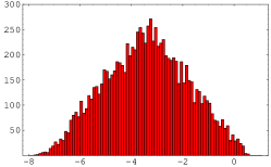
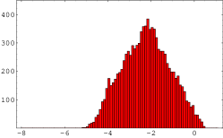
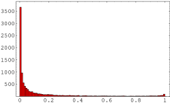
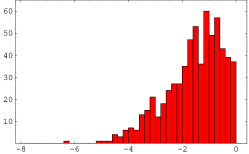
Figure 10 shows the distribution of Yukawa matrix elements for a numerical simulation of this model.
 |
 |
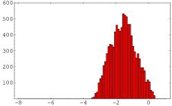 |
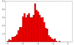
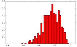
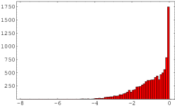
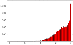
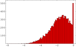
As in the model, the only parameters relevant to these distributions are and , where now is the cut-off scale of the effective theory in 5+1 dimensions. Furthermore, a larger hierarchy is generated when the wavefunctions are more localized, i.e. when is smaller. The key difference from is that the distribution of Yukawa matrix elements is no longer scale invariant. Instead, on the probability density for the largest and the smallest matrix elements is depleted. With regard to the Yukawa eigenvalues and mixing angles, we find that a hierarchical pattern of Yukawa eigenvalues is generated (Figure 11)
 |
 |
 |
 |
 |
 |
 |
 |
 |
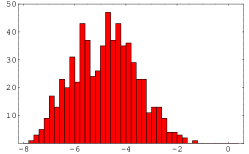
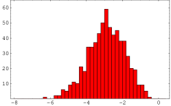
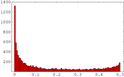
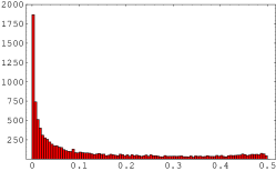
and that the distributions of mixing angles are peaked at but not at (Figure 12). Thus the flavor structure of the quark sector follows from the Gaussian landscape on .
 |
 |
 |
 |
 |
 |
 |
 |
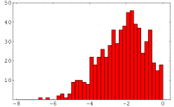 |
Despite the apparent difference between the distribution of the Yukawa matrix elements of the two landscapes (comparing Figure 4 and Figure 10), we see that the distribution of masses and mixing angles are roughly the same when we compare Figures 11 and 12 to Figures 7 and 8. In particular, these distributions all come with a width of about an order of magnitude, and the differences between the distributions from the two toy landscapes is not, statistically, very significant compared to this width. This demonstrates that the flavor structure in the quark sector is a robust feature of Gaussian landscapes.
The biggest difference between the distribution of observables in the two toy landscapes is a more left/right symmetric probability distribution for and on . This is a consequence of the difference in the distribution of individual Yukawa matrix elements, Figure 10 vs. Figure 4. The depleted probability density of the largest Yukawa matrix elements in the Gaussian landscape on results in reduced probability for largest values of and . The distribution of becomes much broader and less peaked at the largest possible value, . This allows the bottom Yukawa coupling to become as small as its measured value rather easily, while still accommodating the measured value of the top Yukawa coupling.
The effects of a possible environmental selection for a large top Yukawa coupling are studied in Figure 11 and in Figure 12, using the cut condition (43) as a crude approximation to the environmental selection effect. The distributions of the mixing angles and are shifted toward smaller angles, just as on . Since the cut condition is in favor of a larger hierarchy between the lighter quarks and the heaviest quarks, smaller and are natural consequences. The inequality also follows from the cut, just like in section 3. The most important difference between the two landscapes may be in the distribution of the bottom Yukawa coupling after the cut is imposed. It was rare that be less than in the lower-right distribution of Figure 7, but a significant fraction is below in Figure 11. Therefore the observed hierarchy may be understood within the context of a Gaussian landscape with an appropriately chosen geometry, especially when there is environmental selection for a large top Yukawa coupling.
For comparison, we also perform a numerical study of a Gaussian landscape defined on . As before, the quarks and Higgs are represented by localized wavefunctions with width . Specifically, on a wavefunction centered at is given by121212Although this wavefunction is not smooth at , this is not of present concern. That is, the purpose of this numerical simulation is not to determine the distribution precisely but to study its qualitative aspects.
| (54) |
Of course, to generate an ensemble of Yukawa matrices the central coordinates of each wavefunction are scanned independently and uniformly over the geometry . Note that like the previously described landscapes, the Gaussian landscape on is characterized by two free parameters, and .
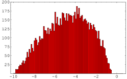
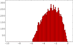
Figure 13 shows the distribution of Yukawa matrix elements for this model.
 |
 |
 |
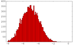
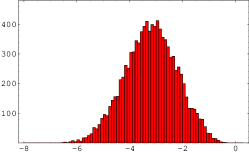
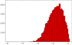
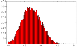
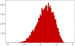
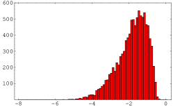
Note that the overall shapes of the distributions are remarkably similar to those in Figure 10, which correspond to . Figure 14 displays the distributions of the three mass eigenvalues for the Gaussian landscapes on and .
 |
 |
 |
 |
 |
 |
These distributions are quite similar between and . We find that the other phenomenological aspects of the Gaussian landscape, discussed above with respect to the geometry , hold true on as well.
5.2 Dependence on Dimensionality and Geometry Independence
Having seen that the hierarchical mass eigenvalues and the generation structure of the quark sector are robust predictions of Gaussian landscapes, the next subject of interest is to understand to what extent the details of distribution functions depend on the internal geometry. Already we have seen slight differences between the Gaussian landscape on and the landscapes defined on and , yet remarkable similarity between the distributions coming from and . We would like to understand where these differences and similarities come from, without having to run simulations on all possible choices of internal geometry. To do this, we recall the analysis of sections 3.1 and 3.2, where the distributions of flavor observables on were understood analytically within the context of the AFS approximation. As we show in this section, this analysis can be generalized to Gaussian landscapes on any geometry of extra dimensions.131313There is also a practical motivation for this approach. The numerical integration time involved with performing overlap integrals on extra dimensions grows very large as the number of extra dimensions is increased; meanwhile generating ensembles of flavor observables involves performing large numbers of these integrals.
Let us consider a -dimensional internal space with local coordinates . Then in the limit where we can ignore the finite size of the internal space the Yukawa coupling matrix is given by
| (55) |
which replaces in (24) for the Gaussian landscape on . Here and are the central coordinates of the quark wavefunctions, relative that of the Higgs. The Yukawa matrix again has the AFS form (25), with suppression factors
| (56) |
replacing (26). In the extra factor (which is not necessarily of order unity) the vectors and are sometimes unaligned, sometimes parallel, and sometimes anti-parallel. This generates a random coefficient to each Yukawa coupling that is statistically neutral in the AFS approximation. We note again that this analysis is valid only when the compactness of the internal space is unimportant and the local geometry can be approximated as a flat -dimensional space. This is equivalent to focusing on only the largest Yukawa matrix elements.
Ignoring the statistically neutral factor , the Yukawa matrix elements are roughly
| (57) |
with scanning a -dimensional space. The natural probability measure is
| (58) |
where is the typical size of the extra dimensions. Indeed, the distribution of the Gaussian landscape on () is flat, c.f. Figure 4, and those of the Gaussian landscapes on and () are linear in at their upper end.141414The distributions on are not as precisely linear for large matrix elements as those on . This can be understood in terms of geometry: has positive curvature while is flat. These results are independent of the value of . The logarithmic range of the distribution of Yukawa couplings scales as .
The distribution of the AFS suppression factors, , can be obtained as in section 3. In more than one dimension the measure (31) is generalized to
| (59) |
where and is the volume enclosed within a distance from a given point. Using (56), it can be converted into a distribution of the AFS suppression factors,
| (60) |
Here, is normalized by , so that ranges from zero to one. For example, for , for and for . The ratio determines the overall logarithmic range of hierarchy, and the volume distribution function controls the shape of the distributions within . It is straightforward to find for a given geometry of extra dimensions; for example, for , and ,
| (61) |
and for the “square torus” ,
| (62) |
These volume distribution functions are displayed in the first row of Figure 15.
The distribution of the smallest, middle, or largest AFS suppression factor is obtained by integrating the other two variables out of the probability distribution
| (63) |
where and we remind that in this notation . The AFS suppression factors for are displayed in the second row of Figure 15. The mass eigenvalues are approximated by , and hence the distribution of is given by a convolution of the distribution function of (third row of Figure 15). The diagonalization matrices for the up and down sectors are determined by three diagonalization angles, which are approximately equal to , . Thus, the distribution of is obtained by integrating the variables out of (63) while keeping the distance (fourth row of Figure 15). Finally, the CKM mixing angles are obtained from the diagonalization angles by approximating the mixing angles to be larger one of in the up sector and the down sector. These are displayed in the fifth row of Figure 15.
 |
 |
 |
 |
 |
 |
 |
 |
 |
 |
 |
 |
 |
 |
 |
 |
 |
 |
 |
 |
Note that the analytical results for the mass eigenvalue distributions (the third row of Figure 15) capture the qualitative features of the numerical results for the Gaussian landscapes on , and very well.
It is now possible to understand why the distributions of flavor observables are quite similar between the Gaussian landscapes on and . All of these distributions are calculated using only the volume distribution function . Although is quite different for these two geometries, as is seen in the first row of Figure 15, a number of consecutive integrations is required to obtain distribution functions for observable flavor parameters. For any AFS suppression factor , the volume distribution function in (63) is not integrated, and thus singularities in the original remain in the distribution of . Nevertheless, the difference in between and is already less evident in the distributions of , (second row of Figure 15), because the integration of two variables out of (63) takes a certain average of . Meanwhile, to obtain the distribution functions of the mass eigenvalues, diagonalization angles, and the CKM mixing angles, each is integrated at least once, and the geometry-dependent information contained in is further smeared out. This is why the distributions of the Yukawa eigenvalues are quite similar between and in Figures 14 and 15. Since the distributions of CKM mixing angles involve a greater number of integrations, these distributions are even less sensitive to the underlying geometry.
The analytical discussion so far explains why the distributions of flavor observables are similar for the Gaussian landscapes on and , but it remains unseen why the distributions of mass eigenvalues of the Gaussian landscape are somewhat different from those of and . Therefore, we now focus on how the number of dimensions in the internal geometry affects the distributions of flavor observables. As we have already seen in the discussion surrounding (58), the number of extra dimensions directly affects the shape of the volume distribution function. Specifically, we find for greater than but near zero. Thus for very small ,
| (64) |
Distribution functions of the masses and mixing angles can be obtained by using the approximations (36) and (38–40), analogous to the analysis earlier in this section. In the limit of large eigenvalues and large mixing angles these distribution functions behave as as
| (65) |
where again and . Note that the behavior of the distribution functions of the mixing angles does not depend on the number of dimensions. The -dependence above is qualitatively confirmed in Figure 15. Because of the slow rising of the distribution function in higher dimensions, the weight of the distribution of is shifted toward larger values, allowing for smaller values of .
As is evident from Figure 15, however, the approximation is valid for only a very narrow range of near zero. Using the explicit form of instead, we can extract another systematic -dependence. The statistical average of plays the role of an AFS charge of the th generation, and determines the hierarchy between the th and th generations. For sequences of geometries with different numbers of extra dimensions—, , and , and , , and —an explicit calculation reveals
| (66) | |||||
| (67) |
This ratio clearly decreases in Gaussian landscapes with a greater number of extra dimensions, meaning that the middle eigenvalue becomes (statistically) closer to the smallest eigenvalue on a logarithmic scale. This also means that in in the AFS approximation the diagonalization angle (and hence the mixing angle) between the first and second generations becomes more significant compared with that between the second and third generations. This tendency is confirmed in Figure 15, where the distribution becomes closer to the distribution for larger . Given that we measure and , this might be regarded as an indication that . Note however that the compactness of extra dimensions affects the distributions of the smallest eigenvalues, and therefore the distributions of observables based on the AFS approximation cannot reliably be used to infer the number of extra dimensions.
Let us now summarize the conclusions of this section. The basic features of flavor in the Standard Model follow from Gaussian landscapes on any geometry of extra dimensions. Specifically, the distribution of Yukawa matrix elements is generally broad and thus there is always hierarchy among Yukawa mass eigenvalues. Furthermore, the up-type and down-type Yukawa matrices are correlated due to the common overlaps of left-handed quark doublets and the Higgs, so that generation structure is always realized. Even in the details of the distribution functions of flavor observables, there is not much geometry dependence. We understand this in terms of the AFS approximation, where all of the geometry dependence is encoded in the volume distribution function . This function is integrated and convoluted many times to obtain the distributions of observables, thus smearing out the original geometry dependence. This means that we cannot learn very much about the geometry of extra dimensions from the observed masses and mixing angles. On the other hand, it appears that we can understand the qualitative pattern of masses and mixing angles without knowing much about the details of the underlying geometry. The number of extra dimensions, however, leaves its footprint on some distribution functions near , because the boundary at remains a boundary in some convolutions. We also find that the mass eigenvalues of the second generation become closer (statistically) to those of the first generation as we increase the number of extra dimensions in Gaussian landscapes.
For various geometries, the volume distribution functions are usually moderately varying functions of over the range . Since the distribution functions of the AFS suppression factors , the mass eigenvalues , and the mixing angles are all derived from , these distribution functions are moderately varying functions of the logarithmic variables , , and . The widths of these statistical distributions are quite broad; to achieve otherwise would require an exponentially steep , which does not happen in Gaussian landscapes. Therefore, the Gaussian landscapes in this article are different from those in [16], where all of the dimensionless coupling constants of the Standard Model have narrow-width Gaussian distributions. This feature of our toy landscapes is traced back to our assumption that the localized wavefunctions become exponentially small as one moves away from the centers of localization.
6 Including the Lepton Sector
Yukawa couplings generated from simple Gaussian landscapes are in good qualitative agreement with the mass hierarchies and small mixing angles in the quark sector. On the other hand, the lepton sector is characterized by large mixing angles and very small neutrino masses. We now turn our attention to how these qualitatively distinct features might be explained within a single landscape model. With the challenges of describing the lepton sector comes the opportunity to predict the probability distributions of three yet-to-be measured observables in the lepton sector: the mixing angle , the CP phase in neutrino oscillations and the mass parameter of neutrinoless double beta decay.
In order to accommodate large mixing angles in the lepton sector, in section 6.1 the Gaussian landscape is extended to include different widths for wavefunctions of particles in different representations. We will see in section 6.4 that the mixing angles can be large indeed, and we also learn that complex (CP violating) phases play a crucial role in determining the distribution of mixing angles (and vice versa in section 6.5). Before studying mixing angles we study the charged lepton mass spectrum in section 6.2. Small neutrino masses are assumed to be generated via the seesaw mechanism, and in section 6.3 we describe how to generate the statistics of the right-handed neutrino Majorana mass terms in Gaussian landscapes. Finally, in section 6.5 we impose some cuts on the statistics generated by a particular version of the Gaussian landscape. This is done to obtain a general feeling for how the probability distributions of yet-to-be measured observables can be affected when distributions conditional on measurements already performed in this universe are considered.
Note that our goal in this section is to find a single theoretical framework that can describe the various flavor structures that are observed; i.e. we aim to identify what subset of landscapes share key qualitative features with the observed flavor structure. Ultimately, the success of the landscape picture will depend on both the existence of phenomenologically viable subsets to the landscape and that these subsets are not too atypical of what is expected from the full landscape, after cosmological and environmental selection effects are accounted.
6.1 Landscapes with Delocalized
In the traditional AFS approach, the large mixing angles of neutrino oscillation and a mild charged lepton mass hierarchy result if the three lepton doublets are not strongly distinguished by the flavor symmetry. For example, an AFS may be broken by a single parameter, with the three ’s strongly distinguished by the symmetry charges while the three ’s are not. Since Gaussian landscapes can mimic an AFS structure in the Yukawa couplings, the idea of different strengths of flavor symmetry breaking for and can be translated into the framework of Gaussian landscapes.
As is seen in sections 3 and 5, the ratio of effective AFS charges for the three fermions in a given representation is determined (statistically) by the Gaussian landscape; we have no freedom to choose these by hand. On the other hand, the overall hierarchy depends on the parameter . So far, for simplicity the parameter has been chosen to be the same for all of the Standard Model wavefunctions; however this parameter can be different for fields in different representations. If the and fields have different width parameters and , then the AFS suppression factors associated with these fields are also different. In such a landscape the single parameter is replaced by three: , and .
If the wavefunctions of the fermions in the representation are not particularly localized, the overlaps between the wavefunctions of the fields and the Higgs boson do not vary hierarchically with the peak locations of the Gaussian wavefunctions. Therefore the Yukawa couplings associated with the three fields are not hierarchically separated when is not much less than . This is along the line of the idea in [17]. On the other hand, such a choice of maintains the hierarchical structure of the masses and mixing angles in the quark sector, when and are chosen the same as before. The main exception is that the hierarchy of the down-type quark masses becomes a little smaller, as we see below, which is actually in good agreement with observation.
6.2 Charged Lepton Mass Spectrum
The masses of the charged leptons derive from the Yukawa interaction
| (68) |
where is generated in analogy to (22), except with a large width to the wavefunction of . In the limit but still , obtains an AFS structure
| (69) |
where is the center coordinate of the wavefunction relative that of the Higgs, and is the broad-width wavefunction of , centered at . Scanning and , the first factor becomes a random coefficient of order unity for all elements of the Yukawa matrix, while the second factor determines the flavor suppression. As the three eigenvalues are roughly the same as the three flavor suppression factors, the distributions of the three eigenvalues, , should be roughly the same as those of the three AFS suppression factors.
Therefore, in the Gaussian landscape on the shape of the distribution functions of the charged lepton Yukawa eigenvalues should be like those in the left panel of Figure 6. We will discuss the overall range of the hierarchy shortly. If we use a common width parameter for and a different common width for ,151515It is an interesting theoretical question whether higher dimensional field theories can give rise to independent scanning of the centers of each of the wavefunctions while preserving the SU(5)GUT symmetric widths. then the distributions of eigenvalues for the down quark sector should be the same as those of the charged lepton sector. On the other hand, the up sector Yukawa couplings involve two fields in the representation, so the distribution of eigenvalues should be closer to those in the central panel of Figure 6 (see section 3 regarding the limitations of applying the AFS approximation to small eigenvalues). The results of a numerical simulation, displayed in Figure 16, confirm that the AFS approximation captures the width-parameter dependence of the distribution functions.
 |
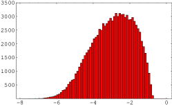 |
 |
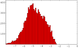 |
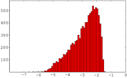 |
 |
Although we do not present numerical results for Gaussian landscapes other than on , the approximate analytic distribution functions for the AFS suppression factors on , , and are presented in Figure 15. In principle one can generalize the analytic discussion to many geometries.
In the limit of broad wavefunctions, (but so that values of remain random), the logarithmic range covered by the charged lepton Yukawa eigenvalues is
| (70) |
For simplicity we choose and to be the same, giving . This is of the result when all of the three widths are the same. In the numerical results of Figure 16, the overall hierarchy in the up sector is slightly larger than that of the down/charged-lepton sectors, consistent with these analytic expectations.
In Gaussian landscapes with , tend to be predicted larger than . This is of course a problem if there is no factor such as in the two-Higgs doublet model. This problem can be solved in two different ways. One is that there may be environmental selection in favor of a large top Yukawa coupling, which makes the observed top Yukawa coupling at the far upper end of its prior distribution, while the bottom and tau Yukawa couplings are not. This scenario does not work very well in the Gaussian landscape on , but it may work in Gaussian landscapes in higher dimensions, since the distributions of the largest eigenvalues receive a high-end tail in extra dimensions (see section 5). The other solution is that the coefficient of overlap integration is smaller for the down-type/charged-lepton sectors than that for the up-type sector. Since the overall hierarchy for the up-type sector is larger than in the down and charged lepton sectors, and because the distributions for the smallest eigenvalues are very broad, this can be done while still maintaining the order of magnitude agreement between and .
It is interesting to note a difference between Gaussian landscapes with large and the AFS models that accomplish neutrino anarchy with very weak AFS for the lepton doublets. In these AFS models, the logarithmic range of the hierarchy in the down-type/charged-lepton sectors is half of that of the up-type sector. On the other hand, this ratio is typically about in the Gaussian landscape on (when ). Of course the precise number may be different for different numbers of dimensions, geometry, and choice of . The difference between AFS and Gaussian landscapes stems from the fact that in the latter the AFS suppression factors associated with are different for the up-type and down-type/charged-lepton Yukawa matrices,
| (71) |
In other words, the flavor suppression factors are not determined by symmetry charges intrinsically assigned to fields in the 10 representation, but depend on the nature of the other fields. In our universe, the down-type/charged-lepton sector hierarchy is not as small as half of that of the up-sector, and Gaussian landscapes have enough flexibility to accommodate this situation.
6.3 Neutrino Mass Hierarchy
Very small neutrino masses are obtained via the seesaw mechanism. Specifically, we assume left-handed neutrino masses derive from the effective dimension-five operators,
| (72) |
which are generated after integrating out heavy right-handed neutrinos, with interactions
| (73) |
In a Gaussian landscape the neutrino Yukawa couplings are generated by scanning the center coordinates of Gaussian wavefunctions, analogous to the generation of . Yet the low energy observables in the neutrino sector also depend on , so we need to introduce some additional assumptions regarding how the Majorana mass terms of the right-handed neutrinos are generated. The traditional approach has been to assume an AFS pattern in the mass matrix . However our Gaussian landscapes are not based on the breaking of any flavor symmetry, but on the overlap integration of localized wavefunctions. Therefore we incorporate this principle into the generation of right-handed Majorana mass terms.
Right-handed neutrinos are singlets under the Standard Model gauge group, but they are charged in more unified gauge groups.161616The term “unified gauge group” is here used in a loose sense. For instance, we do not assume that the Standard Model gauge group is unified as an effective field theory in 3+1 dimensions. For example, unified gauge groups such as , , and contain a symmetry, and the right-handed neutrinos carry non-vanishing charges under this symmetry. In order for charged particles to have Majorana mass terms, some scalar fields on 3+1 dimensions have to be inserted to form gauge-invariant operators, and the expectation values of these scalar fields convert the operators into Majorana mass terms:
| (74) |
The scalar fields or are singlets of the Standard Model gauge groups, but carry charges under whatever symmetry the right-handed neutrinos are charged. In other words, they are moduli fields describing the symmetry breaking of the more unified symmetry.
Since the Majorana mass terms (74) involve vacuum expectation values of scalar fields, the coefficients of the mass terms will involve overlap integrations:
| (75) |
where is the zero-mode wavefunction of the copy of the right-handed neutrino and represents all of the other effects of localization in the extra dimension(s), including the wavefunctions of the symmetry-breaking moduli fields and/or . These fields have nothing to do with the Higgs boson, and hence there is no reason to believe that is localized at the same place in the extra dimensions as the Higgs boson wavefunction. Thus while the AFS structure of all of the Yukawa couplings is due to an overlap between fermion wavefunctions and that of the Higgs, any flavor structure in the Majorana mass term follows from an overlap involving . In particular, unless there is a strong correlation between the wavefunctions of and the Higgs, the flavor structure of the mass matrix is statistically independent of that of the Yukawa matrices.
We study the consequences of this new flavor structure in sections 6.3.1 and 6.3.2. However, before we begin some comments are in order. Our first remark concerns the overall mass scale of the right-handed neutrinos. The overlap integration in (75) sets the flavor structure of , but does not say anything about the overall scale of the symmetry breaking. Thus an extra assumption has to be introduced in order to set the distribution of the overall scale . Even if we know this distribution from theoretical considerations, it may be modulated by environmental selection related to leptogenesis. Therefore we set aside this issue and instead focus only on the hierarchy among neutrino masses and mixing angles in the lepton sector, which can be determined independent of the overall scale of the neutrino masses. This is equivalent to studying a fixed cross section of the full landscape. Our second comment concerns the form of the wavefunctions of the right-handed neutrinos and the symmetry breaking source . To date we have very little knowledge about these fields; yet in a Gaussian landscape their most crucial aspect will be whether in the extra dimensions their wavefunctions are localized or not. Therefore we set aside the theoretical origin of these fields and simply represent them with Gaussian wavefunctions (20), while considering the width parameters and as unknown. By choosing and to be large or small, we can simulate various possibilities. For example, Majorana mass terms generated by world-sheet instantons wrapped on topological cycles may be mimicked by a (possibly multi-centered) Gaussian wavefunction with a small .
It turns out that the mass matrices of the neutrino sector are quite different depending on whether the right-handed neutrinos have localized wavefunctions or not. Therefore sections 6.3.1 and 6.3.2 are separately devoted to these two possibilities. In either case, to generate a statistical ensemble of and the center coordinates of wavefunctions are scanned randomly and independently for , the right-handed neutrinos, lepton doublets, and the Higgs.
6.3.1 Narrow Right-Handed Neutrino Wavefunctions
If right-handed neutrinos have narrow wavefunctions, then the neutrino Yukawa matrix has a structure similar to that of charged leptons. That is, we have
| (76) |
This is (69) with replaced by ; and again the are effectively random coefficients of order unity. The range of the hierarchy is .
Meanwhile, the Majorana mass matrix of right-handed neutrinos is almost diagonal, because the off-diagonal entries are suppressed due to the (statistically) small overlap of wavefunctions between different right-handed neutrinos. If the symmetry-breaking source is also very localized, then the Majorana mass matrix has the approximate structure
| (77) |
where is the width of Gaussian wavefunction of and is the center coordinate of this wavefunction. The positions and are scanned randomly and the largest, middle and smallest become the three eigenvalues of the right-handed neutrino mass matrix. In particular, their distribution functions should be like those of the AFS suppression factors in Figure 6 or 15. For Gaussian landscapes on we have . Results of a numerical simulation on the landscape are shown in the first row of Figure 17, confirming the theoretical expectations so far.
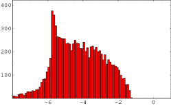 |
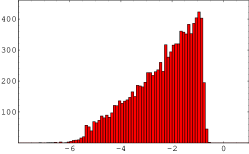 |
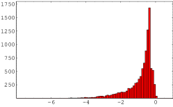 |
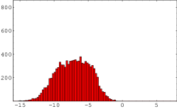 |
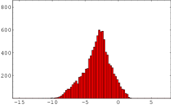 |
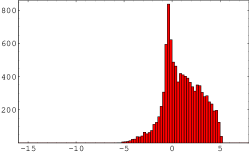 |
If the symmetry-breaking source does not have a localized wavefunction, then we can take to be very large. Then , meaning that there is not much hierarchy among the mass eigenvalues of right-handed neutrinos.
From (73), (76), and (77) the mass matrix of low-energy neutrinos is approximately
| (78) |
Since we introduce no correlation between the Higgs and , we do not expect net statistical cancellations in the ratio . This contrasts sharply with flavor theories that assume an AFS structure for the Majorana mass matrix of right-handed neutrinos. Let the distributions of and be denoted by
| (79) |
where we introduce the new variables ( is normalized to run from zero to one; note that the variable does not necessarily run from zero to one). Because of the form of and in (76) and (77), and are given by the volume distribution function of (60), after re-normalizing the distribution function and rescaling the argument, if necessary. To approximate the distributions of eigenvalues of , we first introduce the variable . The distribution of follows from appropriately convoluting the distributions of and ,
| (80) |
Note that the variable runs from to 2 on . The distribution function can be calculated explicitly once the underlying volume distribution function is known; the results for the Gaussian landscapes on and are shown in Figure 18.
 |
 |
 |
| , | ||
 |
 |
 |
| , |
Using the volume distribution function , we obtain the distributions of the three eigenvalues of by integrating the other two variables out of the combined distribution171717The combined probability distribution of neutrino mass eigenvalues is discussed in [10] for the case with and proportional to a -function. Reference [13] deals with the neutrino anarchy scenario, where the diagonalization effects on the eigenvalue distribution are also taken into account.
| (81) |
where , with . Distribution functions of other observables such as a ratio of low-energy neutrino masses are also calculated from this combined probability distribution. Some examples are displayed in Figure 18. Note that the low-energy neutrino masses tend to have a very large hierarchy, because the distribution function covers the enormous logarithmic range
| (82) |
Specifically, the hierarchies of neutrino Yukawa matrix and the Majorana mass matrix add rather than cancel, c.f. [9, 13]. Even when is very large, low-energy neutrino masses have a hierarchy twice as large as that of eigenvalues of the neutrino Yukawa matrix.
The low-energy neutrino eigenvalues of Figure 17 show a remarkable similarity181818The peak of the distribution of in Figure 17 is near , as opposed to the expected location , shown in Figure 18. The peak of being lower than that of is not surprising. We have seen similar phenomena in Figures 5, 11, 14, and 16. As mentioned earlier, these are likely due to the diagonalization effect. in shape with the corresponding distributions in Figure 18, confirming that the theoretical derivation of distribution functions is fairly reliable. Although results of a numerical simulation on the Gaussian landscape on are not presented here, we have confirmed that the distributions of are similar to corresponding distributions in Figure 18. This success arises because the overlap integration for , and involves only two very localized wavefunctions. Although we have seen around (37) that the analytic distribution functions based on the volume distribution function have a systematic error due to the compactness of the extra dimension(s), the error occurs only for overlap integrations involving three localized Gaussian wavefunctions. Therefore these analytic results can be used to compute distribution functions of flavor observables in the lepton sector in other geometries for which numerical simulation is costly.
The underlying geometry is reflected in the volume distribution functions and . However, these are integrated once to obtain , which smears the effects of geometry. The original ’s are integrated at least once in the distribution functions of , like those of the up-sector eigenvalues. Moreover, the distribution functions of observables such as and involve two integrations over the ’s, such that very little geometry dependence is left in the distribution of the observable.191919The cuspy peaks in the distributions of and on are only logarithmic; the singularity of the original is integrated at least once in each of these. We chose a fine binning in Figure 17 in order to accentuate the logarithmic singularity and emphasize the agreement between the simulation and analytic derivation. When a coarser binning is chosen, the logarithmic singularities are smeared out. Thus, there is not much practical difference in the distributions of ’s whether or or any other geometry is used.
6.3.2 Broad Right-Hand Neutrino Wavefunctions
If the zero-mode wavefunctions of right-handed neutrinos are not localized, i.e. the width parameter is not much less than , then in the neutrino Yukawa coupling only the Higgs has a localized wavefunction. Thus the overlap integral is evaluated around the peak of the Higgs wavefunction. Expanding the other wavefunctions,
| (83) | |||||
| (84) |
we see that the neutrino Yukawa matrix is of the form
| (85) |
where all of the wavefunctions are evaluated at . Note that the first term is a rank one matrix while the additional terms are suppressed by . Thus we obtain a neutrino Yukawa matrix that has the form of the “democratic” mass matrix ansatz, i.e. it is rank one at leading order [18]. Deviations from absolute democracy (i.e. from being rank one) result from the wavefunctions for and not being absolutely flat. The first row of Figure 19 shows the distributions of the three eigenvalues of the neutrino Yukawa matrix. Note that , and have upper limits and there are no effects enhancing the middle eigenvalue; hence the sharp cut-off of the distribution of .
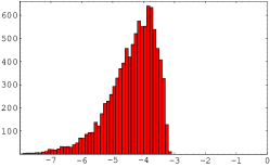 |
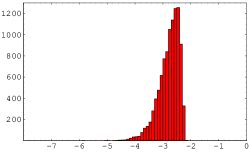 |
 |
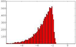 |
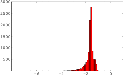 |
 |
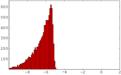 |
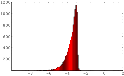 |
 |
An interesting conclusion is that the neutrino Yukawa matrix has a certain amount of hierarchy, no matter how large or small the width parameter of the right-handed neutrinos is. Small Yukawa couplings result from small overlap integrals for localized right-handed neutrinos, or from rank reduction for non-localized right-handed neutrinos.
The Majorana mass matrix of right-handed neutrinos is not hierarchical when the source of symmetry breaking is not localized. Thus in the second row of Figure 19 the distribution of is roughly order unity, and the hierarchy is not more than what is expected from the diagonalization effect.202020We do not have a clear explanation why the distribution of has a long tail toward smaller values. On the other hand, the Majorana masses of right-handed neutrinos become hierarchical when is localized. Then is rank one at leading order, and deviation from being rank one should come at the order of .
The third row of Figure 19 shows the distribution of mass eigenvalues of the low-energy seesaw neutrinos for . The distribution of is sharply cut off at its largest value; this cut-off is presumably traced back to the similarly sharp cut-off of the distribution of the second largest eigenvalue of the neutrino Yukawa matrix . As opposed to when the right-handed neutrinos have localized wavefunctions, it is not as straightforward to develop an analytical understanding of the distribution of seesaw neutrino mass eigenvalues when the right-handed neutrinos have non-localized wavefunctions. Instead, we run numerical simulations with the Gaussian landscape on , using a range of and . We find that the distributions of remain qualitatively the same as in the last row of Figure 19. It is only when is much smaller than that there is a qualitative difference; then the Majorana mass matrix of right-handed neutrinos has hierarchical eigenvalues, and lighter right-handed neutrinos give rise to enhanced values of , erasing the sharp cut-off in the distribution of .
6.3.3 Neutrino Mass Hierarchy in Gaussian Landscapes
It is a robust consequence of Gaussian landscapes on any geometry that the seesaw masses are hierarchical. If the right-handed neutrinos have localized wavefunctions, then the neutrino Yukawa matrix obtains statistically hierarchical mass eigenvalues just like in the analysis of sections 2 and 3. On the other hand, if the wavefunctions are not particularly localized over the extra dimension(s), then the Yukawa matrix always has small eigenvalues due to rank reduction. Because of the absence of correlation between the Majorana mass terms of right-handed neutrinos and the neutrino Yukawa couplings, the hierarchical structure of the neutrino Yukawa matrix remains in the seesaw mass eigenvalues. As a consequence, an inverted hierarchy is unlikely. In addition, it is likely that and
| (86) |
Although Gaussian landscapes predict that the seesaw masses are hierarchical on average, the distribution of mass ratios from Gaussian landscapes are qualitatively different, depending on the choice of the width parameters and . Consider the distribution of for various choices of these width parameters, displayed in Figure 20.
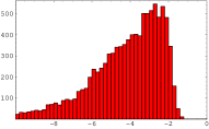 |
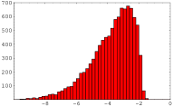 |
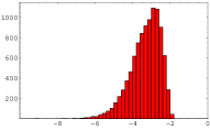 |
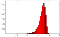 |
| (a) | (b) | (c) | (d) |
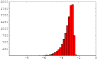 |
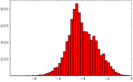 |
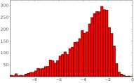 |
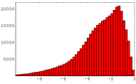 |
| (e) | (f) | (g) | (h) |
| (a): | (e): | ||
| (b): | (f): | , , | |
| (c): | (g): | , on | |
| (d): | (h): | , |
When neither the right-handed neutrino nor the symmetry-breaking wavefunction(s) are localized, the distribution of is sharply cut off at around , seen in Figure 20 (d) and (e). In this case there is no chance to accommodate the observed value,
| (87) |
If is large and the wavefunction is strongly localized in the extra dimension(s), then the distribution of has a tail extending upward as in Figure 20 (f). This is because of the previously mentioned enhancement in the seesaw mass matrix—due to small eigenvalues in the Majorana mass terms of the right-handed neutrinos—which erases the sharp upper bound on . The distribution in Figure 20 (f) barely covers the observed value (87), but the width parameters may be chosen a little differently to provide better coverage in the tail of the distribution. Yet even in this scenario, the distribution of is peaked at a value much smaller than the observed value (87). If environmental selection factors (such as those associated with leptogenesis) and weight factors associated with cosmological evolution are in favor of such an outlier, then this scenario may be acceptable. Otherwise, one should conclude that this scenario is not a good approximation to the actual landscape governing the flavor structure of the multiverse.
It is left to consider localized wavefunctions for the right-handed neutrinos. The approximate distribution of is derived analytically in this scenario, and plotted in the right column of Figure 18. Regardless of the geometry this distribution covers a broad logarithmic range, with the greatest weight toward the largest value, . These analytical distributions capture the qualitative features of Figure 20 (a), (b), and (g) very well, with one important difference: the distributions in the numerical results fall off to almost zero for . This behavior of the numerical results is presumably due to the diagonalization effect, a phenomenon first mentioned in section 3.2 and subsequently referred to with regard to Figures 5, 11, 14, 16, and 17. This reduced weight in the probability distribution functions at means that this scenario is also in conflict with the observation (87).
There is an important caveat, however, which is that the diagonalization effect changes as the real-valued matrices that we have dealt with so far are generalized to complex-valued matrices. See the appendix of [13], for example. Figure 20 (h) is based on an extended version of the Gaussian landscape on (presented in section 6.4) that includes complex phases. The diagonalization effect clearly has much less impact on the distribution function of , and this distribution extends almost all the way up to . Thus we find the scenario with localized wavefunctions for the right-handed neutrinos is compatible with the large value observed for , assuming the Gaussian landscape contains complex phases.
6.4 Mixing Angles and CP Phases
We introduced non-localized wavefunctions for the fields in because we expected this to result in large leptonic mixing angles. However numerical simulation reveals that the mixing angles, particularly , are still very small, as can be seen in the left panel of Figure 21.
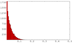 |
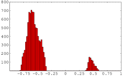 |
 |
 |
 |
The figure presented here is a simulation using small and ; but the distribution is confined near no matter how small or large these parameters are taken to be.
The distributions of and in Figure 21 explain why, contrary to our expectation, we failed to get large . An SO(3) matrix acts on the left-handed charged leptons when diagonalizing the charged lepton Yukawa matrix , and acts on the left-handed neutrinos when diagonalizing the seesaw mass matrix . Their (2,3) components are large, just as we expected. Yet the mixing angle of atmospheric neutrino oscillation, the (2,3) component of , is small due to a precise cancellation between the large and . This cancellation is not a new phenomenon. The democratic mass matrix ansatz, originally applied to the quark sector, yields small mixing angles through this precise cancellation.
To obtain large mixing angles, some modification is needed to prevent this cancellation. We replace the real-positive valued Gaussian wavefunctions in (20) by Gaussian wavefunctions with a winding complex phase:212121This form for the wavefunction is not without motivation, c.f. the discussion surrounding (163). However, we use this wavefunction only as one of the simplest means to introduce complex phases into Gaussian landscapes. There are more complicated, more sophisticated, and possibly better justified ways to introduce complex phases into Gaussian landscapes, or landscapes based on extra dimensions in general. It would be interesting to explore such models that include complex phases to study the correlation between the induced CP violation and the distribution of other observables. However this subject is beyond the scope of this paper. We restrict attention to (88) and find that even this simple model is sufficient to obtain large leptonic mixing angles, when is large.
| (88) |
introducing a new parameter . For simplicity we use the same value of for all of the wavefunctions in the overlap integrations, . The wavefunction of does not have to be the complex conjugate of that of , since for example in the framework of section 7 these wavefunctions are not just scalars but have more complicated internal structure.222222We have checked that one can obtain results very similar to those presented in this section, but taking , if one also allows for non-universal values of .
As seen in Figure 22, using this form of wavefunction makes and complex, and their phases decrease the likelihood of a precise cancellation in . Furthermore, these complex Gaussian wavefunctions introduce CP violation into the flavor physics. Meanwhile, this introduction of complex phases has little effect on the distributions of charged fermion mass eigenvalues. This can be understood analytically by tracing the discussion in the preceding sections with the wavefunction (88). We also confirmed this result by running numerical simulations. The diagonalization effect is not taken into account in the theoretical arguments, but in practice this matters only for the neutrino mass distribution, and we have seen that this improves the agreement with observation.
On the other hand, introducing complex phases dramatically changes the distributions of mixing angles. Figure 23 shows the distributions of the three leptonic mixing angles resulting from a numerical simulation.
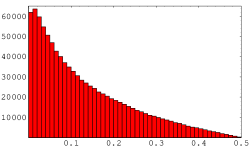 |
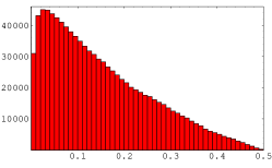 |
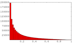 |
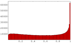 |
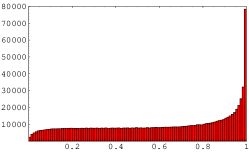 |
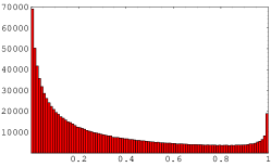 |
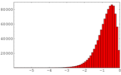 |
 |
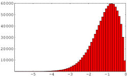 |
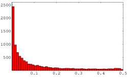 |
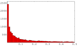 |
 |
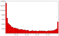 |
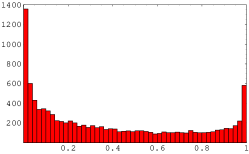 |
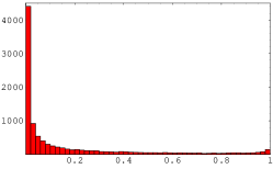 |
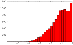 |
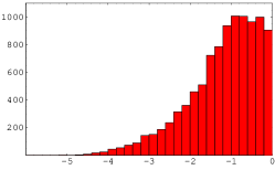 |
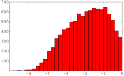 |
We see that the mixing angles of solar and atmospheric neutrino oscillations, and , are likely to be any value between and . Distributions of the oscillation amplitudes are almost flat for both of these mixing angles. Peaks at maximal mixing come from the Jacobian [13]. Comparing the distributions of between Figure 23 and Figure 21, we see that the introduction of complex phases (and hence CP violation) is an essential ingredient in obtaining large (and even maximal) mixing angles in neutrino oscillations.
The mixing angle can also be of order unity, which is similar to the situation in neutrino anarchy [9, 13]. In the U(3)-invariant measure to be expected in neutrino anarchy, however, the distribution function of is peaked at , and vanishes at . Thus all three mixing angles in the lepton sector are likely to be large. In particular, according to neutrino anarchy using the U(3)-invariant measure, about 60–90% of the statistics are already excluded by the current experimental limit on [9, 13]. In the Gaussian landscape on , on the other hand, the distribution is weighted more toward . As we see in section 6.5, only about 30% of the statistics have been excluded.
For comparison, the distributions of the quark mixing angles are also simulated in the same Gaussian landscape and are presented in Figure 24. We see that the complex-valued Gaussian profiles maintain small mixing angles when the overlap integrals involve narrow Gaussian widths for ’s and the Higgs. Interestingly, simply choosing different widths for particles in the and representations, in the presence of large CP-violating phases, allows for very different flavor structures between the quark and lepton sectors. Thus pursuing a microscopic description behind the statistical distributions of Yukawa couplings has enabled us to go beyond the results of [9, 10].
The distributions of the CP violating phases are also shown in Figure 25.
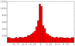 |
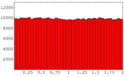 |
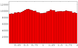 |
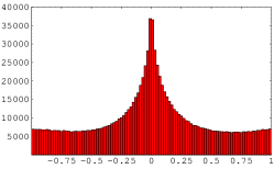 |
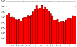 |
 |
| (no cut) | () | () |
Our parametrization of the CKM and leptonic mixing matrices and is quite standard:
| (92) | |||||
| (99) |
where and . The Majorana mass phases of the neutrinos, , have almost flat distributions. On the other hand, the distributions of the two other CP phases, and , have peaks at on top of otherwise flat distributions. We have not studied where this structure comes from. The scatter plot of in Figure 22 reveals some structure—the scatter is dense in some places and thin in others—and the peaks at in the CP phase distributions may have something to do with this structure, which presumably originates from the specific form of the wavefunction (88). If this guess is correct, then the peak plus flat structure in the CP phase distributions is likely to be an artifact of the particular way in which we have introduced complex phases into this landscape. It would be interesting to see how the CP phase distribution changes when complex phases are introduced in a different ways, but this subject is beyond the scope of this paper. Although we expect that the peak structure may deform, disappear, or become less significant, we consider it unlikely that the flat part of distribution would disappear and that CP phases would be predicted to be very small. If this expectation is correct, then these landscapes are consistent with the measured value of the CP phase in the quark sector.
6.5 Conditional Probabilities
The neutrino sector has three observables yet to be measured, , and . It would be interesting if landscape approaches to understanding flavor could make predictions for these observables. We have developed our Gaussian landscapes so that all the observables measured in this universe are not too atypical. In this section, we use the Gaussian landscape on , with the set of parameters , , and , as an initial example to explore what kind of predictions can be obtained from this approach.232323This Gaussian landscape has 19 scanning parameters, corresponding to the center coordinates of the wavefunctions of the quarks, leptons, Higgs boson, and symmetry-breaking field(s) . Meanwhile, this landscape now predicts distributions for all 22 flavor parameters. Although this implies that the landscape makes three precise (zero-width) predictions; this is a result of our arbitrary choice to consider parameters such as , , and as fixed. Specifically, these predictions disappear when these parameters also have probability distributions around the values we fixed. Therefore we do not pursue the possibility of a truly predictive Gaussian landscape.
The mixing angle is typically of order unity, and there is no reason to expect from this Gaussian landscape that it is very small. Indeed, the current experimental limit has excluded a significant fraction of the ensemble of vacua:
| (100) |
Nevertheless, the experimental limit is not very strong and so a significant fraction of vacua—67% of the total ensemble in this Gaussian landscape—sits within the experimental bound. On the other hand, future experiments are expected to have a sensitivity down to about . The probability that is too small to be measured by such future experiments is rather low within this Gaussian landscape; we find
| (101) |
The second yet-to-be measured parameter is the CP phase of neutrino oscillations. The probability distribution of this is displayed in the bottom left panel of Figure 25. Finally, neutrinoless double beta decay measures , where
| (102) | |||||
| (103) |
The second term of (102) is roughly
| (104) |
after using (86) and (87). Once is measured, the second term of (102) can be estimated. Yet we still need to know the last term, , to make a prediction for . The Gaussian landscape distribution of is found in the top right panel of Figure 26.
We can ask more specific questions to further constrain the probability distributions of these three observables in universes like ours. That is, when making predictions for future measurements, we can condition the probability distributions based on quantities that we have already measured, as opposed to using the a priori probability distributions in the landscape. However, if we were to impose the current experimental limit on all lepton flavor parameters, an enormous numerical simulation would be required, since most of the simulated universes would not pass the cut. This does not imply that our universe is very atypical, only that the present experimental error bars are small. Therefore, for practical reasons we employ much looser experimental cuts242424One might consider these cuts as a tool to study the effects of possible cosmological or environmental selection in the multiverse, just like a large top-Yukawa cut (43) was employed in section 3 in an attempt to study the impact of environmental selection in favor of a large top Yukawa coupling. Here, however, we know of no evidence that the weight factors are in favor of the range of parameters selected by the cut conditions –.
| (105) | |||||
| (106) | |||||
| (107) | |||||
| (108) |
and study whether these cuts influence the distributions of , and .
Table 2 shows how the probability to measure changes depending on whether or not the cut conditions – are imposed.
| 61% | 75% | 78% | 77% | 94–95% | 79% | 87% | % |
The loose cuts – have a significant impact on the prediction. Among all the samples that are consistent with the current experimental limit on , 40% of them are below . However, after imposing various other experimental constraints, –, only a few percent have . Therefore, for the wavefunction parameter choices used in this section, the Gaussian landscape on predicts a very high probability of measuring in future experiments in our universe.
| – | ||
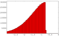 |
 |
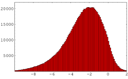 |
| () | () | (no cut) |
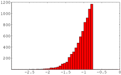 |
 |
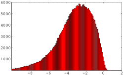 |
| () | () | () |
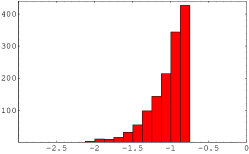 |
 |
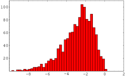 |
| () | () | () |
When is large, there is a good chance to observe CP violation in neutrino oscillation experiments. The a priori vacuum statistics for this parameter are peaked at (bottom left panel of Figure 25). However the distribution of changes as some of the cuts – are imposed. The impact of these changes is clearly visible when the mixing angles of both the solar and atmospheric neutrino oscillations are required to be large; then the peak of the CP phase distribution is significantly reduced (bottom middle panel of Figure 25). This is reasonable, since complex phases play a crucial role in avoiding cancellation between large mixing angles in and . In scatter plots in the – plane (Figure 26), we see that the distribution of the CP phase becomes uniform after cuts – are imposed. Therefore, after conditioning distributions based on our loose “experimental cuts,” both and the CP phase become more likely to be larger, and hence more likely to be discovered in future experiments.
The loose cuts – also have some impact on the distribution of (Figure 26). The condition alone, requiring be large, removes almost all the distribution as well. Examining the samples that pass all cuts –, we find that
| (109) | |||||
| (110) |
where the uncertainty comes from limited statistics in the numerical simulation. Therefore, it is very unlikely that is so large as to be significant next to the first term in . Hence this landscape predicts and
| (111) |
where .
We have seen that the loose cuts – have a significant impact on the distributions of , and . This study gives us a feeling for how much landscape predictions can change when various weight factors multiply the simple vacuum statistics, or when various experimental measurements are used to condition predictions based on what we know about our universe. Details about these predictions will depend on the specific weight factors or how severely the experimental cuts are imposed. However, as we have seen, the impact of these cuts can be understood qualitatively, and we expect similar results for similar weights or cuts.
Although the width parameters of , , and the Higgs have been optimized to fit the observed data, there is still much room left to change and (or even or how complex phases are introduced into the Gaussian landscape). If and/or were chosen slightly larger, then the distribution of covers a smaller range, and the cut would have less impact while the other three cuts on the mixing angles would remain as important. Since it was cuts and , respectively, that had impacts on the distributions of and , the “predictions” on and would not be affected very much. On the other hand, since the cut was important in dragging the distribution of upward, the distribution of may shift downward for a slightly larger or . Thus the “predictions” in this section should be interpreted carefully, with these and other caveats252525For example, landscapes of Yukawa couplings originating from super Yang–Mills theory in higher dimensions have basis-independent distributions, but Gaussian landscapes—simplified versions of the former—do not (see section 7). This situation is compared to the basis independent implementation of neutrino anarchy in [13] and the original implementation in [9]. The latter predicted anti-correlations between mixing angles in the lepton sector, but these angles are uncorrelated in the former. Thus some of the correlations in Gaussian landscapes may be spurious. Nevertheless, the disappearance of correlations in the basis-independent neutrino anarchy was related to invariance under the U(3) group. Unless there is a similar underlying symmetry, we expect that the probability distributions of Gaussian landscapes are not qualitatively different from those of higher dimensional gauge theories. in mind.
7 Yukawa Couplings from Super Yang–Mills Interactions
In the preceding sections, we introduced a number of toy models, collectively termed Gaussian landscapes, to generate statistical ensembles of Yukawa matrices. The pairing and generation structures of the CKM matrix along with the large mixing angles of the lepton sector were successfully explained as random selections from these ensembles. The most crucial ingredient to these Gaussian landscapes was that Yukawa couplings are given by overlap integration of localized zero-mode wavefunctions on extra dimensions. The correlation necessary to account for generation structure arose because the wavefunctions of quark doublets and the Higgs are relevant for both the up-type and down-type Yukawa matrices. We also introduced a number of additional assumptions concerning which parameters are scanned and which not. In this section we give give greater theoretical consideration to these assumptions.
Consider a supersymmetric Yang–Mills theory on a higher dimensional manifold. The internal space of extra dimensions is denoted . The gauge group is chosen so that it contains a subgroup such as of the Standard Model or a unified gauge group such as . The gauge fields of the theory may have non-trivial configurations on as long as they are stable (and hence satisfy the equations of motion). Such a gauge field configuration can break the underlying gauge symmetry down to .
In this context the fields () in become the gauge fields of the Standard Model or the unified theory. Meanwhile, the Kaluza–Klein spectrum of () in , under the gauge field background, may have zero modes (i.e., massless modes), and such quantum fluctuations become scalar fields in the four-dimensional low-energy effective theory. Gauginos in may also have zero modes; since a spinor in a higher-dimensional space is bi-spinor of the Lorentz group and , and the zero-modes of the Dirac equation on become massless fermions in the effective theory. These low-energy scalar and spinor fields may be charged under the Standard Model or unified theory gauge group, or they may be singlets under these gauge symmetries. This is worked out by decomposing the adjoint representation of into pieces irreducible under . Charged fields arising in this way may well be identified with quarks, leptons and the Higgs.
Fermion and scalar fields arising from the super Yang–Mills fields in higher dimensions have Yukawa couplings in the low-energy effective theory. To see this more explicitly, consider the Lagrangian of a super Yang–Mills theory in higher dimensions:
| (112) |
These three terms become the kinetic terms for the vector, scalar, and spinor fields in the effective theory. Meanwhile, the gauge coupling constant of the low-energy effective theory is
| (113) |
where is the volume of the internal space. When the zero-mode wave functions and are normalized such that
| (114) |
then canonically normalized kinetic terms result when the low-energy fields are related to those in the higher dimensional theory by
| (115) |
Then low-energy Yukawa couplings originate from the gauge interactions of gauginos
| (116) |
with the effective Yukawa coupling constants given by
| (117) |
Thus the low-energy Yukawa couplings are given by overlap integrations, just as in (22), where now is interpreted as the gauge coupling constant of the super Yang–Mills theory.
Having specified the origin of the quarks, leptons, and their Yukawa couplings, we know what the underlying gauge group has to be. For , super Yang–Mills interactions of or give rise to all of the Yukawa couplings of the quarks, charged leptons and neutrinos [19]. For the Pati–Salam group , is sufficient. When the Heterotic or string theory is compactified on a real six-dimensional compact manifold, we obtain Yukawa couplings in this way; for example, with and a six-dimensional manifold for the string theory. In some compactifications of the Type IIA string theory (or supergravity on eleven dimensions) and Type IIB string theory (or F-theory), the Yukawa couplings of quarks and leptons arise from open string interactions. For example in the Type IIA string theory with an intersecting D6–D6 system, with quarks and leptons localized at the intersections of D6-branes, the Yukawa couplings are generated by spanning a world sheet to three intersection points with D6-branes connecting them. However, some of these compactifications can be understood as a certain limit of Heterotic compactification; this is the essence of string duality. Thus the toy models that we use to calculate Yukawa couplings can capture certain aspects (and maybe all) of these compactifications as well. Therefore, the numerical analyses of this paper can be used to understand the statistics of flavor structure arising from a large region of the string theory landscape.
If quarks, leptons and the Higgs originate from a super Yang–Mills theory of containing , and the Yukawa couplings from the super Yang–Mills interaction of , then we cannot arbitrarily assume the following:
-
•
the shape of zero-mode wavefunctions—these must be solutions to the equations of motion.
-
•
the number of zero-modes—this is determined by the topology of the geometry of the internal manifold and of the gauge field configuration on .
-
•
the number of independent parameters that freely scan—only moduli parameters, i.e. deformations of the manifold and gauge field configuration that cost no energy, are scanned.
The possible restrictions above were ignored in the preceding sections, as we introduced assumptions instead. In this section we discuss when such assumptions are justified, when they are not, and when not what one should expect instead. In sections 7.1 and 7.2 we provide a pedagogical and bottom-up introduction to ideas that motivated us to assume Gaussian zero-mode wavefunctions with center coordinates that scan over the landscape. Most of the content of these sections is not particularly new, and the intended audience is non-string theorists. We use the remainder of this section to describe what the toy models of sections 3, 5 and 6—i.e. Gaussian landscapes—mean in the context of the string theory landscape.
Before we proceed, let us comment on the basis-independence of observables. The Standard Model has three independent fermions in a given representation, and the Yukawa matrices transform under a group that preserves the canonical kinetic terms of the fermions. Observables such as mass eigenvalues and mixing angles also do not change under this transformation. Thus, any probability distribution of Yukawa matrices in a landscape-based theory should be either invariant under the U(3) transformations, or defined only for classes of Yukawa matrices equivalent under the U(3) transformations. This basis independence follows in landscapes that derive from super Yang–Mills interactions. Indeed, the zero modes—i.e. the solutions of massless Dirac equations in a given representation—form a vector space, the rank of which gives the number of generations. One should find an orthonormal basis of the vector space , such that the metric of the kinetic term is given by
| (118) |
and use the zero-mode wavefunctions of the basis vectors to calculate the elements of Yukawa matrices through
| (119) |
The above U(3) transformations correspond to basis transformations of the vector space of zero modes. Here the U(3) basis transformations correspond to no more than choosing different descriptions of the same vacuum,262626Only the vector space composed of solutions to the zero-mode equations of motion have these U(3) “symmetries;” the interaction terms—which are trilinear (not quadratic) in fields on a given background—do not respect these flavor symmetries at all. and the actual statistical elements of the landscape correspond to vacua, not Yukawa matrices. Thus, any landscape generating vacuum statistics through the overlap integrals of zero-mode wavefunctions is basis independent.272727The U(3)-invariant Harr measure for mixing angles follows in basis independent landscapes [13] when and (, , and ) are independent. In landscapes derived from overlap integration, however, there are correlations between the relevant matrices, and hence the mixing angles do not follow the Harr measure.
The Gaussian landscapes introduced in sections 3, 5 and 6 are meant to be simplified versions of (subsets of) the landscape that derives from string compactification. Because of the way we have simplified the landscape—scanning the center coordinates of zero modes completely randomly and independently—the basis independence of the landscape from string compactification is lost in our Gaussian landscapes. However if the Gaussian landscapes are regarded as tools to acquire a better understanding of flavor physics in the landscape from string compactification—and this is certainly our attitude—then the lack of basis independence in Gaussian landscapes is itself not a major problem.
7.1 Domain Wall Fermion and Compactification of Field Theories on Six Dimensions
Domain Wall Fermion
It is well known that a chiral fermion in a four-dimensional effective theory is localized at a domain wall in a five-dimensional theory [20]. Consider a fermion in a five dimensions,
| (120) |
where on and on . A chiral zero mode is localized about the point where a background scalar field configuration equals zero, its wavefunction being
| (121) |
When the background configuration is approximated by a linear function , then the zero-mode wavefunction is approximately Gaussian:
| (122) |
Thus the Gaussian profile follows from the zero-mode equations of motion rather easily.282828On a domain-wall background, the zero-mode wavefunction is Gaussian in the middle of domain wall, where is approximately linear, and decreases exponentially outside the wall, where is nearly constant.
However, when the direction is compactified into , the scalar field must be periodic. If hits zero with a positive slope times along , it does with a negative slope times as well. Thus, when there are chiral left-handed zero modes in the low-energy effective theory, there must be chiral right-handed zero modes as well, and the net chirality is zero. Furthermore, the background field configuration should satisfy its equation of motion, but kink–anti-kink configurations are in general not stable.
Domain Wall Fermion from a U(1) Gauge Theory
These problems are addressed if is not a scalar field. Consider for example a U(1) gauge theory on a six-dimensional spacetime with a charged fermion:
| (123) |
where the gamma matrices are chosen to be
| (124) |
When the gamma matrices are chosen as above, the SO(5,1) spinor consists of four four-dimensional Weyl spinors, . In a basis where and
| (125) |
the six-dimensional Dirac equation is given by
| (126) |
where and . Let us focus on the Weyl spinor . When is ignored, this spinor’s Dirac equation is the same as the five-dimensional equation above—that is enters the equation just as does in (120). Thus acts like a mass parameter for a five dimensional fermion. Chiral fermions are localized where “vanishes,” just like with the domain wall fermion. Below we make more precise what we mean by “vanishing” .
Let us consider a U(1) gauge theory compactified on , with coordinates and having periods and . Suppose that is linear in and is constant:
| (127) |
The field strength is constant, and satisfies an equation of motion , where . There is no issue of kink–anti-kink instability (however see the discussion at the end of this section, where another instability is discussed). Since is part of a gauge field, it must be periodic in only up to a gauge transformation. Since a gauge transformation shifts by , and can differ by an integral multiple of . Therefore (and the field strength ) have to be quantized:
| (128) |
It follows from the index theorem that there are
| (129) |
chiral fermion zero modes. Because of the linear configuration of the effective mass term , zero modes correspond only to left-handed spinors (if ), and net chirality is obtained in the low-energy effective theory.
Fermion Zero-Mode Wavefunctions: I
It is easy to find one of the zero-mode wavefunctions referred to above:
| (130) |
just like a domain wall fermion. This zero mode is localized where the effective mass parameter is zero; . Since a gauge transformation shifts by and shifts by , the center coordinate of the Gaussian profile can always be chosen within the interval . To obtain the other zero modes, note that a Kaluza–Klein momentum in the direction effectively shifts the Wilson line :
| (131) |
Hence the remaining zero modes are
| (132) |
for (mod ). The center coordinates of these Gaussian zero modes are at
| (133) |
The width of the Gaussian profile is
| (134) |
It has been assumed that the width of Gaussian wavefunctions can be parametrically smaller than the size of the extra dimension in the direction. This is equivalent to
| (135) |
where parametrizes the shape of . In the analysis of section 3 (the Gaussian landscape on ), we found was sufficient to reproduce the hierarchy of the quark sector. This translates to when .
Fermion Zero-Mode Wavefunctions: II
In fact the fermion zero-mode wavefunctions on are known exactly; the approximate form (132) is valid only when can be ignored, i.e. when is so small that only one Kaluza–Klein momentum is relevant at a time. Let us take a detour here to see the form of the zero-mode wavefunctions when is not satisfied. First, we note that the fermion obeys a twisted periodicity condition,
| (136) |
just like,
| (137) | |||||
| (138) |
The wavefunctions of the chiral zero modes, which satisfy , are given by [21]
| (139) | |||||
| (140) |
for (mod ). Here we have defined
| (141) |
In addition, is a theta function defined by
| (142) |
The wavefunctions (140) form an orthonormal basis when the normalization constant is
| (143) |
If and , then the zero-mode wavefunction (139) receives dominant contributions only from the consecutive values of for which is between and . For other values of the last factor is suppressed by a power of when . Thus the wavefunctions are linear combinations of Gaussian profiles localized in the direction, centered at .
If , then the expression given in (139) is not useful to obtain an intuitive picture. Using a modular transformation of the theta function,
| (144) |
(140) can be rewritten
| (145) | |||||
| (146) |
where
| (147) |
When , all but one term in the series expansion of the theta function (142) are suppressed by powers of , while the leading order term is a Gaussian wavefunction localized at . This is the solution we obtained in (132).
Although we have chosen a particular gauge (127), the localization pattern of fermion zero modes does not depend on the choice of gauge: the U(1) gauge transformation on fermion fields is not more than a phase multiplication. Although we chose to be dependent while is not dependent, the fermion zero modes exhibit a localization in when , and a localization in when . Thus the width of the Gaussian profiles is given by (134) in both cases, and is smaller than and , respectively. As expected, despite the – asymmetric gauge choice, the localization pattern is not – asymmetric. The modular transformation property of theta function guarantees this.
Note that when and are comparable, the zero-mode wavefunctions are neither Gaussian nor localized. For more about zero-mode wavefunctions on tori, see for example [22].
Zero Modes of Various Fields in Different Representations
At the beginning of this section, we advertised the idea that all of the fermions, the Higgs boson and the gauge bosons are unified into a super Yang–Mills multiplet of a gauge group that contains the gauge group of the Standard Model or some unified theory. Let us describe this idea a little more explicitly, using the language of compactification with a U(1) gauge field background. Consider a super Yang–Mills theory (a parallel description applies to Pati–Salam unified theories with and ). Among the generators of the U(6) symmetry, U(1) field strengths on are introduced along
| (148) |
and a couple of U(1) factors commute with these field strengths, and these are identified with the Standard Model gauge group. Gauginos in the block and in the block are in the and representations of , just like the quark doublets and the anti up-quarks. Thus, the corresponding zero modes of the gaugino can be identified with these Standard Model fields. Meanwhile, the Higgs boson may arise from in the block. Then the gauge interaction of the gauginos in (119) gives rise to the up-type Yukawa coupling: following the commutation relations of U(6) (c.f. [23]) we have,
| (149) |
The Yukawa couplings are then calculated by overlap integrals of the zero modes.
The U(1) flux in U(6) is given by , with each of () given by , as in (127) and (128). One has to set the field strengths , and so that there are three quark doublets and three anti-up-quarks in the low-energy spectrum. This means that
| (150) |
The three Gaussian zero-mode wavefunctions of quark doublets and anti-up-type quarks are localized at
| (151) | |||||
| (152) |
This is an illustration of the picture described in the introduction to this section. We started from U(6) super Yang–Mills theory on and broke the U(6) symmetry by turning on a gauge field background, so that an gauge symmetry is left unbroken along with some U(1) factors. Furthermore, the gauge-field background generated chirality in the low-energy spectrum, and determined the shape of the zero-mode wavefunctions (which are Gaussian when or ). Wilson lines () are chosen arbitrarily, yet the field strength satisfies the equation of motion. Thus, these constants determine the zero-mode wavefunctions, and hence the observables that arise from the Yukawa matrices. If the Wilson lines are scanned, the peaks of the Gaussian zero modes are also scanned, and hence the Yukawa couplings are scanned. Since the zero modes of quark doublets and anti-up-type quarks depend differently on the Wilson lines—see (151) and (152)—the peak positions of the wavefunctions of different representations are scanned independently from one another.
Problems
The compactification of super Yang–Mills theory reproduces certain aspects of the Gaussian landscape on , but it also has serious problems. The easiest problem to identify involves the sum rule on the chirality. Because of the simple relation , we have
| (153) |
implying that the low-energy spectrum contains up-type Higgsinos and fermions in a representation conjugate to that of the up-type Higgsinos. One encounters a similar sum rule in any compactification on a smooth two-dimensional manifold with U(1) field strengths; thus this is too simple a framework to provide both a realistic spectrum and Yukawa interactions.
A more serious problem is that the constant gauge field configuration in U(6) is not stable. Although this configuration satisfies the equations of motion, this only means that it is a stationary point of the action. In fact, the equations of motion of the gauge field in the and blocks are given by
| (154) | |||||
| (155) |
Here is the Laplacian on the – plane. The positive and required for the proper quark chirality implies that the low-energy complex scalar fields coming from have negative mass-squared. Therefore the constant U(1) gauge field configuration is not stable on . It is stable only when , which yields no net chirality.
Complex Valued Wavefunctions
In section 7.2 we move on to discuss more complicated compactifications of supersymmetric Yang–Mills theory in search of frameworks for constructing Gaussian landscapes that avoid the above problems. For the remainder of this section, however, we digress to explore how CP-violating phases can be introduced into these landscapes. We look at the simplest geometry imaginable—compactification on —considering that the essence of obtaining CP-violating phases will not be lost in more complicated frameworks.
Real-valued Gaussian wavefunctions never yield complex phases in the Yukawa matrices or CP-violating phases in the quark and lepton mixing matrices. Although the zero-mode wavefunctions have phase factors , these do not end up as complex phases in the Yukawa matrices. The first factor cancels in the integrand of the overlap integration. For example, consider the symmetry breaking model. The up-type Yukawa operator is neutral under any one of () symmetries, and this ensures that the phase factor in the quark-doublet wavefunctions is canceled by the factor in the anti-up-quark wavefunctions. As for the second phase factor , recall that the overlap integration is carried out on both the and coordinates. This phase factor is a plane wave associated with Kaluza–Klein momenta, and these momenta are conserved in compactifications. Therefore in any matrix element given by overlap integration on , these plane wave phase factors cannot yield complex phases.292929Kaluza–Klein momenta conservation leads to an approximate texture in the Yukawa matrices. When only the leading term in the series expansion of the theta function is kept for each of , , and , a given quark doublet has a non-vanishing Yukawa matrix element with only one anti-up-type quark. All of the other matrix elements are suppressed by at least , which arises after sub-leading terms in the series expansion of the theta function are included. On the other hand, when compactifying on generic manifolds there is not necessarily any Kaluza–Klein massless U(1) gauge field and its corresponding conserved Kaluza–Klein momenta. This is why we consider that the Yukawa texture from Kaluza–Klein momenta conservation is an artifact of torus compactification, and have ignored it in the Gaussian landscapes of earlier sections.
However, there is a simple way to obtain complex phases in Yukawa matrices without considering more complicated geometries. So far we have assumed is rectangular; that is the two independent periods,
| (156) |
are rectangular. In other words, using the complex coordinate we have,
| (157) |
with a pure imaginary given by (141). When is not pure imaginary (while keeping the metric ), zero-mode wavefunctions have more complicated complex phases, as we see explicitly below.
We now use the gauge field configuration,
| (158) |
where and are the real and imaginary parts of , and
| (159) |
The fermion fields satisfy the twisted periodicity conditions in (136) for the periods in (157). The zero-mode wavefunctions (140) are modified and become
| (160) | |||||
| (161) |
where and are the complex conjugates of and , respectively. To see the behavior of these wavefunctions when is small (roughly equivalent to ), we use (144). Dropping the sub-leading terms in the series expansion of the theta function and maintaining only the and terms in the exponent, we have
| (162) |
The factors and may cancel in overlap integration. The second factor,303030Here we have used ; see (135) and (147).
| (163) |
has a complex phase when . This phase will not cancel with overlap integration on , which is why we used this second factor in the zero-mode wavefunctions in the Gaussian landscape of section 6.4.
7.2 Doubling — Compactification of Field Theory on Eight Dimensions
We have seen that the zero-mode wavefunctions are localized and Gaussian in a compactification with a constant U(1) gauge field background, when or vice versa. Thus, when the is doubled and compactification with a constant U(1) background is considered, the zero-mode wavefunctions are localized and Gaussian in two of the four directions, when is short in the other two directions. As we will see in this section, in compactification the net chirality of various representations is no longer subject to a linear sum rule, and the instability problem in the compactification can be avoided when the gauge field configuration satisfies an anti-self-dual condition. Note that sections 7.2 and 7.3 discuss supersymmetric Yang–Mills theory on eight dimensions as a possible origin for Gaussian landscapes, but not because we regard a theory on eight dimensions as a candidate for a fundamental theory. Instead, these sections are intended to provide a step-by-step introduction to ideas that formal theorists are already familiar with, but with minimum technicality. Later, in sections 7.4 and 7.5, we consider a realistic framework for building Gaussian landscapes.
Fermion Zero Modes in Anti-self-dual Gauge-Field Background
We label the four coordinates of and the circumferences in these directions are denoted . We assume that these directions are all orthogonal, i.e. the internal metric is
| (164) |
On this , we introduce a U(1)2 gauge field configuration embedded in SU(2):
| (165) | |||||
| (166) |
The field strength is constant and satisfies the equation of motion. Moreover, this configuration is stable when the anti-self-dual condition is satisfied; that is when
| (167) |
A Weyl fermion in the fundamental representation of the SU(2) has zero modes on . To see this, we use the following gamma matrices:
| (168) |
A Weyl fermion on eight dimensions consists of four-dimensional Weyl fermions , where is a “color” index running in the case of a fermion in the fundamental representation of SU(2). Corresponding to the different choices of and , the Dirac equation on with the gauge field background (166) has zero modes in :
| (169) |
Likewise, there are also zero modes in :
| (170) |
When and , all of these wavefunctions are approximately Gaussian in the – plane, since the wavefunction is a product of Gaussians in the and directions. Two zero modes, one in and the other in , are localized at each of
| (171) |
The width of all of these zero modes is in the direction and in the direction. The anti-self-dual condition (167) implies that the two widths and are equal, as was assumed in the Gaussian landscapes of section 5.
Absence of a Chirality Sum Rule
The two serious problems of compactification with a U(1) gauge field background derived from instability of the gauge field configuration and the sum rule satisfied by the chirality of different representations. The anti-self-dual condition (167) addresses the first issue in (or in any four-dimensional manifold) compactification, while in what follows we see that there is hope to resolve the second issue in four-fold compactifications as well.
The chirality sum rule on derived from the Yukawa interactions being consistent with the gauge symmetry of an underlying group . Therefore, to discuss the existence of such a sum rule313131To be precise, chirality on four dimensions is not obtained from a super Yang–Mills theory on eight dimensions compactified on with an anti-self-dual gauge field configuration. This is because the super Yang–Mills multiplet contains a pair of Weyl fermions with opposite chirality. When a zero mode is found in () in a Weyl fermion , another Weyl fermion with the opposite chirality, , also has a zero mode (). The chirality we refer to in this section concerns compactification of ten to six dimensions, which has nothing to do with the chirality on four dimensions. As we explain later, however, the chirality on six dimensions in compactification has non-linearity, which is shared by chirality on four dimensions in any six-dimensional compactification. This “chirality” is discussed in the context of compactification because this is the simplest system with this non-linearity. on , we must consider constraints from the underlying gauge symmetry whose super Yang–Mills interactions give rise to the Yukawa couplings of quarks and leptons. Here we consider and . contains a subgroup
| (172) |
The symmetry is unbroken when a background gauge field on is contained within . We use the U(1)2 gauge-field configuration in (166), embedded in the SU(2) factor, and introduce a U(1) gauge field background in the U(1)6 factor, given by
| (173) |
with another anti-self-dual condition .
The irreducible decomposition of the Lie algebra,
| (174) | |||||
| (175) |
shows that contains both and , candidates for the and multiplets, respectively. The above decomposition refers to the the subgroup in the first line, and in the second line. Gauge interactions of gauginos may in principle give rise to the four-dimensional up-type Yukawa couplings323232Let us first consider how gauge indices are contracted. The SU(5)GUT indices of the two fermions are contracted with the SU(5)GUT totally anti-symmetric tensor, and the contraction is symmetric under the exchange of the two. On the other hand, the internal gauge indices of are anti-symmetric as the above interaction is neutral under the underlying gauge symmetry , when the contraction is in the first term of the right-hand side of . Generally, gauge indices are contracted anti-symmetrically under the exchange of the two zero modes in the representation. This should be the case because the gauge indices are contracted through the structure constant of a Lie algebra in (119). Spinor indices are contracted symmetrically under the exchange of ’s; both the SO(3,1) contraction of left-handed spinors in four dimensions and the contraction of spinor indices of SU(2) SO(4) in the internal space are anti-symmetric. Therefore the combined contraction of gauge (anti-symmetric) and spinor (symmetric) indices is anti-symmetric. This is expected since the gauginos in eight dimensions are Grassmann variables. ,333333 The Higgs scalar should, then, originate from the complex scalar of a super Yang–Mills multiplet on eight-dimensions. However, because of the supersymmetry, preserved in compactification with an anti-self-dual gauge field configuration, the existence of massless Higgs boson implies that its super partner, a vector field in the same representation, should also be massless. This implies that the symmetry is not broken down to . As we have seen, compactification with an anti-self-dual configuration has so many problems that it cannot be regarded as a realistic framework for landscapes. Our goal in section 7.2 is to introduce field-theory ideas that apply to many compactifications, using the language of compactification.
| (176) |
As a quick check, note that in the algebra does not vanish. The coefficients (Yukawa matrix elements) are calculated by the overlap integration of the zero-mode wavefunctions, picking up a pair of and . If the compactification preserves supersymmetry, a complex scalar and a chiral fermion in a chiral multiplet have the same wavefunctions on the internal manifold. Therefore the wavefunction of the Higgs boson is Gaussian, whenever the Higgsino wavefunction is Gaussian.
The number of zero modes is calculated in terms of the flux quanta and . Up-type Higgsinos in low-energy spectrum are zero modes of the Dirac equation involving a U(1) gauge field . Therefore the number of up-type Higgsino zero modes is
| (177) |
Light fermions in the 10 representation are zero modes of a Dirac equation with gauge field . The number of zero modes is
| (178) |
with the first term coming from those in and the second term from those in . We have four (discrete) parameters to choose by hand to fit the desired multiplicities of the fields in the two different representations, and .
The discussion so far has not been realistic. The above multiplicities count only the number of hypermultiplets of supersymmetry in four dimensions. We have also commented in footnote 33 that the Higgs scalar field in the up-type Yukawa couplings should belong to an vector multiplet. However, it will now be easy to take one more step and triple to a compactification of a super Yang–Mills theory in ten dimensions. Chirality on four dimensions is obtained in compactifications, and the net chirality of a given representation is cubic in discrete parameters specifying the fluxes on . No sum rule holds among the chirality of various representations, since they are not linear functions of the flux parameters. As more flux parameters are involved, it is easier to fit the multiplicities of fields in various representations. It is also known that one of the gauge background stability conditions is (in compactifications preserving supersymmetry), and the compactification has instability because only one term contributes to the left-hand side, with no chance of cancellation. Hence this instability is an artifact of the compactification. contains , and therefore the algebra that led to the up-type Yukawa couplings still works in . Thus super Yang–Mills theories of ten dimensions compactified on six-dimensional internal manifolds can be a good theoretical framework for building Gaussian landscapes.
Scanning of the Center Coordinates
Before closing this section, let us see how the localized wavefunctions behave as the constant gauge field background on changes. We already know that all the zero-mode wavefunctions are approximately Gaussian if and . The center coordinates of these wavefunctions depend on the Wilson lines and , according to
| (179) | |||||
| (180) | |||||
| (181) |
where the coordinates in the first line are those of up-type Higgsino(s), while the second and third lines are those of the 10 fermions, with the second and third lines coming from and , respectively. Note that the coordinates of the second and third lines show different dependences on the Wilson lines. Thus as the Wilson lines are scanned, the localized fermions in the 10 representation of change their relative positions. We see that the scanning of Wilson lines allows for more than the center-of-mass scanning of Gaussian peaks to zero-mode wavefunctions in compactification. In the Gaussian landscapes we scanned the peak positions of Gaussian wavefunctions without considering any correlations or constraints among the various peak positions. The above situation is still far from this treatment, but so far we have only scanned the Wilson lines. In section 7.3 we see that there are other stable gauge field configurations, and as more gauge field configurations are scanned, correlation will be lost among the Gaussian peak positions. This is the rationale behind the absence of correlations in the Gaussian landscapes.
7.3 Instanton Moduli and Random Peak-Position Scanning
Instanton Moduli
We have now seen an explicit example of a stable gauge field background on parameterized by Wilson lines. In general, stable gauge field configurations allow for continuous deformations, such as Wilson lines, and the parameters of such deformations are called moduli. As for gauge field configurations on a four-dimensional manifold, we know that those satisfying the anti-self-dual condition satisfy both the Yang–Mills theory equations of motion and the stability condition. Such gauge field configurations, called instantons, are known to have numerous moduli parameters; the Wilson lines on are just a subset of the instanton moduli parameters. Therefore we now consider what happens when the instanton moduli parameters are scanned. Our primary interest is to explore the moduli space of stable gauge field configurations on a six-dimensional manifold, as this is relevant to the compactification of the Heterotic string theory. However, to warm up we first study instanton moduli on a four-dimensional manifold.
The symmetry breaking model in section 7.2 generates the up-type Yukawa couplings. As long as a background configuration of gauge field is contained in its subalgebra, the symmetry remains unbroken. Note that the gauge field configuration does not have to be pure Abelian over the entire as is assumed in (166). The gauge field configuration in (166) can be replaced by any one of the SU(2) instanton configurations343434 The number of fermion zero modes is given by the topology of the gauge field configuration and of the geometry, as in the case of compactification. It follows from the index theorem that the number of fermion zero modes in a representation of a gauge-field background is (182) where is the classes of and is in the first Pontrjagin class. This expression is valid for an arbitrary four-dimensional manifold . The first term on the right-hand side is equal to , that is it is proportional to the instanton number . As long as the instanton number remains the same, the net chirality does not change for any instanton configuration. See the text for the definitions of and . on . The ’t Hooft solution is an SU(2) instanton configuration on a flat Euclidean four-dimensional space [24]; it has moduli parameters, where the instanton number is topological and defined by
| (183) |
here fund. stands for fundamental representation, is an arbitrary representation, and “ch2;R” stands for the second Chern character in the representation . The gauge-field configuration in (166) has instantons. Meanwhile, the ’t Hooft solution,
| (184) |
describes isolated instantons, centered at with a size . Here, label the three generators of and is the eta symbol of ’t Hooft. Thus there are indeed moduli parameters. In addition to these five moduli parameters per instanton, there are three more moduli parameters describing how an instanton solution is embedded within the group . Thus, there are (roughly) moduli parameters for the SU(2) -instanton configuration.
On a compact four-dimensional manifold , the number of instanton moduli parameters of a gauge group is given by [25]
| (185) |
where denotes the Dynkin index in the adjoint representation (also known as the dual Coxeter number), is the Todd classes, and is the dimension of . When is , and . Apart from the second term, which is associated with compactness of the four-fold , the first term reproduces the result of — moduli parameters. The second term corresponds to an obstruction for lifting isolated instantons into an anti-self-dual configuration over all of the (c.f. [26]). The Wilson lines on the compactification of section 7.2 are part of the instanton moduli. However unlike the Wilson lines of , which are associated with a non-trivial , most of instanton moduli here are not strongly associated with the specific geometry of . Thus the existence of instanton moduli is very robust.
Wilson lines as Instanton Moduli Parameters
So far it has not been clear how the Wilson lines on are related to the instanton moduli parameters, such as and , in the ’t Hooft solution (184); in particular the constant-field configuration does not have a well-defined center. To see explicitly that the Wilson lines actually correspond to instanton center coordinates, ADHM data [27] and the Nahm transformation [28] are useful.
The ADHM formalism [27] allows one to parametrize the moduli space of an instanton configuration on a flat space . A set of parameters called ADHM data describes all possible instanton gauge-field configurations and, in turn, the data can be extracted starting from the gauge field configuration. For simplicity, we consider only the -instanton configurations of an SU() gauge group. Among the data is an matrix-valued . This part of the data is extracted by
| (186) |
where () are the zero-mode wavefunctions of a fermion in the fundamental representation of the SU() gauge group. Since the zero-mode wavefunctions are determined by the gauge field configuration used in the Dirac equation on , the data carry some of the information of the gauge field configuration. It is known that the data corresponding to the ’t Hooft solution are
| (187) |
Thus the data provide a way to extract “center coordinates” from the instanton gauge field configuration. When one considers a family of instanton gauge field configurations by modifying
| (188) |
the fermion zero-mode wavefunctions change according to
| (189) |
Therefore the data are also extracted by
| (190) |
The gauge field configuration (166) is already in the form (188), and the zero-mode wavefunctions of the fermions in the fundamental representation are also already provided. The corresponding data, now calculated by integration on , not , are ([21] and references therein)
| (191) |
Therefore the Wilson lines and can be regarded as center-of-mass modes of the instanton center coordinates in the appropriate limit of the instanton moduli space.
Scanning over Instanton Moduli Space
If the moduli parameters of the instanton configurations are scanned randomly (according to some measure), the gauge field configuration is determined for each choice of moduli parameter, as are the zero-mode wavefunctions. In the symmetry breaking model of section 7.2, fermions in the 10 representation of in the effective theory are zero modes of fermions in the representation of an instanton background. As the moduli of an instanton are scanned, zero-mode wavefunctions of the fields in vary. The center coordinates of these wavefunctions will be scanned almost randomly, since the instanton center coordinates can be chosen arbitrarily in (184). The zero modes of a fermion in the representation are not classified into the zero modes in and those in . The instanton configuration is contained in a Cartan subgroup for only limited points in the instanton moduli space; for generic points in the moduli space the symmetry is completely broken and the distinction between and is lost. In general each zero mode has non-zero wavefunctions in both and . This means that there is no selection rule in the Yukawa couplings; if some zero modes were exclusively in and all others were in , then the Yukawa couplings would have involved only a pair of zero modes, one from each group.
The Gaussian landscapes of sections 3, 5, and 6 extracted these features. In particular, we applied these features to all of the fields in the Standard Model. Certainly the Higgs wavefunction is determined only by a gauge field background of an Abelian symmetry in the symmetry breaking model; therefore the complexity (and variety) of instanton field configurations of non-Abelian symmetries has nothing to do with the scanning of the Higgs field’s center coordinate. But this is just an artifact of choosing to be minimal for the up-type Yukawa couplings. For a larger underlying gauge symmetry , such as , the Higgs is regarded as a zero mode of a field in the representation in symmetry breaking due to an instanton. Gaussian landscapes are based on an expectation that the variety of stable gauge-field configurations is so rich that the random scanning of gauge field moduli results in (approximately) random and independent scanning of the center coordinates of the zero-mode wavefunctions.
One will notice here that the three Gaussian zero-mode wavefunctions in a given representation do not necessarily satisfy the orthonormal condition (118), when the center coordinates are chosen completely randomly. Our approach has been to try to implement the rich scanning of gauge field moduli in Gaussian landscapes at the cost of giving up basis independence. Since the orthonormal condition is violated especially when two center coordinates coincide, the probability distribution functions of the smaller eigenvalues of a Yukawa matrix in Gaussian landscapes may become unreliable as the approach the largest possible value, in the notation of this paper. Although the center coordinates of two instantons can coincide, the two zero-mode wavefunctions associated with them should be properly modified so that they remain orthogonal. This modification is not taken into account in the Gaussian landscape. It is a yet-to-be tested question in string theory whether the gauge field moduli are such that the random scanning of center coordinates is a relatively good approximation or not, and if not how the correct distribution functions of observables would deviate from the predictions of Gaussian landscapes.
Non-Gaussian Wavefunctions
We here note that zero-mode wavefunctions are not always Gaussian for arbitrary choice of gauge field moduli parameters. In fact, when the sizes of instantons in the ’t Hooft solution (184) are much smaller than the typical distance between the instanton centers , the ’t Hooft solution is a collection of isolated BPST instantons. Fermion zero modes are localized around the instanton centers , and their wavefunctions decay in as a power of the distance , not exponentially. Unless the size parameters are extremely small, however, overlap integration using these non-exponential wavefunctions tends to be larger than the – required to match the quark and lepton Yukawa couplings of the first generation.
There are also situations where zero-mode wavefunctions decay linear-exponentially, rather than as a power law. In section 7.1 (7.2), we discuss only () compactification, where no topological 1-cycles (2-cycles) can shrink while keeping the volume of () finite. However in more complicated geometries there are topological cycles that can do this. When a U(1) flux is introduced on such a topological 2-cycle, and if for some reason the 2-cycle shrinks, then symmetry breaking by the U(1) flux can be localized in extra dimensions, c.f. [29]. This contrasts with the situation in sections 7.1 and 7.2, where the symmetry-breaking U(1) field strength is spread out homogeneously over the extra dimensions. If the symmetry breaking U(1) flux is localized at a point in the extra dimensions, then fermion zero-mode wavefunctions decay linear-exponentially, with the exponent proportional to the distance from the symmetry-breaking source. Depending on the choice of parameters, the linear-exponential wavefunctions may or may not lead to as large a hierarchy as that which results from Gaussian wavefunctions. It would be interesting to study the effects on Yukawa-related observables of such a localized symmetry breaking source, but this is beyond the scope of this paper.
To date, there has not been much investigation into what part of the moduli space of gauge field backgrounds is more statistically weighted in flux compactification. It might be discovered that the statistic distribution is more weighted in regions that lead to Gaussian (or possibly linear-exponential) wavefunctions, so that large hierarchy among Yukawa couplings follows as a likely consequence. The other possibility is that environmental selection in favor of a light charged lepton (and/or quarks) enhances the statistical weight for such regions. We do not know which, if either, possibility is correct. However, for the landscape to account for the observed hierarchical patterns in the mass eigenvalues and mixing angles, we must assume one of these possibilities. As long as either of these possibilities is correct, then Gaussian landscapes should not be too terrible an approximation (or an effective description) of the landscape formulated by a super Yang–Mills theory on higher-dimensional spacetime.
7.4 -Fibered Compactification and M(IIA)-theory Dual
In this paper we present numerical simulations of Gaussian landscapes involving only extra dimensions. This is due to limited computational resources, not because there is any theoretical motivation to study landscapes involving . Indeed, more interesting would be to study Gaussian landscapes on , since such a model would directly simulate (some fraction of) the landscape of Yukawa couplings in string theory. A Gaussian landscape on a three-dimensional manifold corresponds to Heterotic string theory compactified on a six-dimensional manifold that is a -fibration over . To clarify, when one says that a -dimensional manifold is a -fibration over a manifold , this means that the manifold locally resembles almost everywhere in . For example, and in sections 7.1 and 7.2 are trivial examples of and -fibered geometry. Here is called a base manifold, and a fiber.
Suppose that a six-dimensional manifold is a -fibration over a three-dimensional manifold . We choose a coordinate system locally, so that the direction is parametrized by and a local patch of by . When the periods of in its three directions, , , and , are small compared with the size of (that is, the cubic root of the volume of ), then a stable gauge field configuration on is approximately described by fields that vary slowly on the coordinates of . Fermion zero modes are localized at points on where all of , and vanish. As long as , , and are all small, the zero-mode wavefunctions are approximately Gaussian [30]. Although is not globally the same as or , the local structure of —its -fibration—is sufficient to determine the approximately Gaussian zero-mode wavefunctions. Wavefunctions away from the Gaussian peak will depend on details of the global structure of , but the wavefunctions are exponentially small in this region. Assuming a Gaussian profile with a fixed width for wavefunctions is surely a very crude approximation, but it might suffice as a zeroth order approximation. A Gaussian landscape on a -dimensional manifold assumes that the moduli of stable gauge field configurations are so rich that the center coordinates of various fields are scanned (almost) randomly and independently. The results of section 5 provide a qualitative picture of how the distributions of observables depend on the base manifold .
The most important parameter in a Gaussian landscape is the ratio of the Gaussian width to the size of the extra dimensions, . For example, the overall hierarchy of Yukawa couplings is proportional to on a logarithmic scale. As we have seen in section 7.1, this ratio is proportional to . This is generalized to
| (192) |
As in sections 7.1 and 7.2, the volume of the fiber has to be sufficiently smaller than that of the base manifold in order for hierarchy to be generated. It is an interesting question whether this property can be understood within string theory, not as a phenomenological requirement.
The Heterotic string theory compactified on a -fibered geometry corresponds to an eleven-dimensional supergravity compactification on a -fibered geometry (this is an intersecting D6–D6 system of the Type IIA string theory) in the limit of small . Thus, Gaussian landscapes on three-folds for various values of are intended to simulate a class of vacua of string theory that interpolates between the Heterotic theory and M-theory (ignoring stringy corrections). The expression in Type IIA language (the last term) in (192) is known. Numerical simulation can tell us the value of that fits to the observed pattern of masses and mixings, which suggests the approximate value of (192) for the vacuum of our universe.
7.5 -Fibered Compactification and F-theory Dual
The analysis of Gaussian landscapes in section 5 may help one understand the landscape of Yukawa couplings of Heterotic compactification on a -fibered geometry. Let us now consider a six-dimensional manifold that is a -fibration over a four-fold . Let parametrize a local patch of the -fibration and a local patch of . Fermion zero modes are localized on a two-dimensional sub-manifold (called the matter curves) on so that the gauge fields and both vanish [31]. Furthermore, their wavefunctions around the matter curves are approximately Gaussian in the two transverse directions determined by and . The existence of the two transverse directions in which zero-mode wavefunctions are Gaussian is quite similar to the Gaussian landscapes. One can determine the value of that fits the observed hierarchy of masses and mixing angles, which might then be used to infer for the -fibered geometry. This class of vacua interpolates Heterotic string theory and F(type IIB string)-theory.
There are also some features that are not captured by the Gaussian landscapes. Suppose that varies along , and along ; at least it is possible to choose a coordinate system on locally so that this happens. Then a matter curve is along the () directions. However the net chirality of a fermion depends on , the gauge field along the matter curve. Therefore zero-mode wavefunctions should have some dependence, but no such dependence is taken into account in the Gaussian landscapes. Moreover, the global geometry of matter curves may be complicated in , and they can intersect one another, but the Gaussian landscapes ignore this as well. The behavior of zero-mode wavefunctions on a -fibered geometry and the geometry of the intersection of matter curves must be studied further to determine whether the Gaussian landscapes can be useful in studying the landscapes of Yukawa couplings with -fibered compactification.
8 Conclusions
This decade has seen the emergence of a major debate: to what extent is nature fundamentally uniquely prescribed, for example by symmetries, vs. to what extent nature results from the statistics of a huge landscape of vacua, modified by cosmological and environmental selection. For the Standard Model symmetries play a key role, but for physics beyond the Standard Model the question remains largely open. Unified gauge symmetries have striking achievements, for example a simple interpretation of the quantum numbers of a generation and a precise numerical prediction for the ratios of the measured gauge couplings. For quark and lepton flavor, however, the picture offered by approximate flavor symmetries (AFS) is much less compelling, lacking both theoretical simplicity and significant successful predictions. Although the AFS description of flavor is apparently well suited to give an understanding of the hierarchical nature of charged fermion masses and the CKM mixing matrix, it comes with too much flexibility: with an appropriate choice of charges and symmetries any pattern of flavor can be generated.
In this paper we introduce Gaussian landscapes as some of the simplest landscapes in extra dimensions that can account for flavor. Particles are assumed to possess localized (Gaussian) zero-mode wavefunctions over some geometry of extra dimensions, and the Gaussian landscape consists of independently scanning the peak position of each of these wavefunctions. Small flavor-symmetry breaking parameters are replaced by small overlap integrals of these wavefunctions on the extra dimensions. Localized zero-mode wavefunctions in extra dimensions are a natural expectation, and may have a more elegant realization than Higgs potentials for flavor symmetry breaking. We claim neither precise predictions nor do we present a compelling top-down theoretical model, rather we present the patterns of flavor that emerge from these simple toy landscapes, the features of these extra-dimensional landscapes that are relevant to the flavor problem, and how these landscapes might be realized within the context of string theory.
In the simplest Gaussian landscape describing the quark sector, where all quarks and the Higgs have a universal Gaussian wavefunction (but with independently scanning center coordinates) over a single extra dimension with geometry , we find the three major characteristics of quark flavor: a hierarchical distribution of quark masses, pairing structure (the -current approximately connects distinct pairs of quarks), and generation structure (the electroweak pairing connects the heaviest up-type quark to the heaviest down-type quark, and similarly for the middle and lightest quarks). The relevant probability distributions are shown in Figures 4 and 5 and result from inputting just two parameters: a universal constant of order unity setting the scale for overlap integrals and a universal constant setting the width of Gaussian wavefunctions relative the size of the extra dimension.
The flavor structure of the quark sector can also be obtained from AFS using two free parameters. For example, by hypothesizing an approximate symmetry with a leading Yukawa coupling of order unity and others suppressed by various powers of a small symmetry breaking parameter . However there is a crucial difference. In the AFS case one must carefully choose the charges of each of the fifteen fermions of the Standard Model. A huge variety of mass patterns could be accommodated by suitable charge choices. In the Gaussian landscape no such choices are made. Each of the fifteen fermions is treated symmetrically. They differ only by the location of their Gaussian wavefunction, and these are scanned randomly over . Thus the hierarchies arise purely from statistics; they cannot be changed as they do not involve any free parameters beyond and .
While the above accomplishments of the Gaussian landscape on are striking, there are certain features that are less than ideal. Although they are peaked, the probability distributions for flavor parameters are quite broad, as can be seen in Figure 5. At half maximum, the deviation from the peak value is typically an order of magnitude. Thus the statistical nature of the landscape prevents us from making precise predictions. We find that this order of magnitude width is also typical of Gaussian landscapes in more than one dimension. The landscape makes no distinction between up and down sectors. This is a problem for explaining the observed large mass ratio, in particular because on the distribution for the top and bottom masses is narrower than for the other generations and also because it is peaked near the maximum value. Thus even if there were a selection effect favoring a heavy top quark, the observed bottom mass would still be somewhat unlikely.
One possibility to resolve this shortcoming is to replace the effective coupling with two parameters: one for the up sector that is about an order of magnitude larger than the one for the down sector. It would be interesting to find the landscape origin for such a “” factor. Another possibility is that the shape of the mass distribution is a special feature of the landscape. We find that this is the case. In the landscape, where Gaussian wavefunctions are distributed at random over the surface of a (square) torus, the distribution is wider, as shown in Figure 11. The same result holds for Gaussian landscapes on and . A selection for a heavy quark, for example for electroweak symmetry breaking, could then more easily account for the mass ratio. For any number of extra dimensions, we can analytically compute the Yukawa probability distribution near maximal values, and we find that it is suppressed as the dimension increases, strengthening this interpretation of the ratio.
Although flavor symmetries play no fundamental role in Gaussian landscapes, small overlap integrals may allow AFS to emerge in the low-energy theory. For example, if , and have narrow Gaussian profiles with centers that are well-separated from each other, then AFS that act on and will emerge at low energy. We have found that Yukawa matrices have the form expected from Abelian AFS, namely , if the Higgs width is not too wide and if the Yukawa coupling is not too small. As the separation between the Higgs and quarks approaches the scale of the extra dimension, effects associated with the periodicity of the wavefunctions destroys the AFS form of the Yukawa coupling. Nevertheless, the AFS approximation aids in understanding the numerical results, and we have used it to compute approximate analytic distributions for the AFS factors , the quark mass eigenvalues, and the CKM mixing angles.
This strategy is particularly useful for understanding Gaussian landscapes on higher dimensional geometries where numerical integration requires greater computational resources. Analytic results for the geometries , , , and have been obtained and the distributions are compared in Figure 15. We find that the qualitative predictions of the Gaussian landscape on remain intact. One important feature is that, independent of the dimension , the AFS distribution functions and flavor observables are found to be polynomial or logarithmic functions of or . By comparing numerical distributions of flavor parameters in Gaussian landscapes on and , we have investigated the importance of the shape and curvature of the extra dimensional manifold. We find some differences in the details, but the more striking are the similarities, as seen for example in Figure 14.
Large leptonic mixing angles suggest that in the low-energy theory no AFS emerges for the lepton doublets , implying that the Gaussian widths for are comparable to the size of the extra dimension(s). Since the fermion mass hierarchies are smaller in the down and charged lepton sectors than in the up sector, we economize on parameters and assume that the widths preserve an symmetry, with . The smallness of the neutrino masses suggests that there is no light right-handed neutrinos, such that the light neutrinos are Majorana and the origin of neutrino masses involves the breaking of symmetry. In the seesaw mechanism this implies Majorana masses for heavy right-handed neutrinos. In the Gaussian landscape we expect Gaussian profiles for both and the breaking fields. The center of the breaking is not expected to be correlated with the center of breaking, leading to a very different statistical character for the Majorana and Dirac mass matrices of neutrinos.
We find that the physics of neutrino masses and mixings is quite different depending on whether the profile for is narrow or wide. In the case that it is narrow, localization leads to significant hierarchies in the eigenvalues of both the Majorana and Dirac matrices. In theories based on AFS these hierarchies cancel in the light neutrino mass matrix, but in the Gaussian landscape these hierarchies add. The result is that is typically too small to agree with observation, unless perhaps if strong selection effects are important. For wide profiles, the neutrino Yukawa and Majorana matrices take on a democratic form, and again have hierarchical eigenvalues. If the profiles are sufficiently wide, is always less than the observed value, as shown in Figure 19. Similar difficulties arise with the lepton mixing angle . Although a large width for the lepton doublets leads to large 23 rotations to diagonalize the charged and neutral lepton mass matrices, these large angles cancel so that the physical mixing angle is typically small, as shown in the numerical simulation of Figure 21.
These difficulties, that and are typically much smaller than the values observed, are both solved by a remarkably simple observation. In order to account for CP violation in the quark sector a complex phase must be introduced to the Gaussian profile. Using the simple profile of (88), we find the following results for the Gaussian landscape on :
-
•
Previous results for distributions of charged fermion masses are preserved, for example Figure 16 is essentially unchanged for CP-violating Gaussian landscapes.
-
•
The generation structure of the quark sector is preserved (Figure 24).
-
•
The CKM phase is of order unity (Figure 25).
-
•
Large leptonic mixing angles and are obtained (Figure 23).
-
•
The large observed value for the neutrino mass ratio is not atypical (Figure 20(h)).
The distributions of flavor observables on Gaussian landscapes are typically broad. However, given the experimental measurement of some subset of flavor observables, the conditional distributions for the remaining observables in our universe changes significantly. We find that even quite loose cuts on the measured neutrino parameters are sufficient to considerably sharpen the predictions for the leptonic mixing angle, , and the neutrinoless double beta parameter, , within a particular Gaussian landscape; see Figure 26 and (111), respectively. Furthermore these cuts lead to a prediction of large CP violation in neutrino oscillation as shown in the last row of Figure 25 and in the scatter plots of Figure 26.
When a supersymmetric gauge theory is compactified on an internal manifold, quarks, leptons and the Higgs boson may originate from gauginos and the components of gauge fields with polarization along the internal manifold. Their Yukawa interactions originate from the gauge interactions of the gauginos, while the Yukawa coupling constants are calculated by overlap integration of zero-mode wavefunctions over the extra-dimensional space. Wavefunctions become Gaussian when the extra-dimensional manifold is a torus fibration, and the fiber is small relative to the base. Thus, Gaussian landscapes fit very well into this framework—compactification of a supersymmetric gauge theory on a torus-fibered manifold.
The ratio , which controls the hierarchy, roughly reflects the ratio of the torus fiber size to the base size in Heterotic theory language. We now know the value of that is good for quark and lepton phenomenology, but it remains an open question why such a value has been selected from all the possibilities in the landscape (or if it represents a typical subset of the landscape). Indeed, there is no theoretical motivation to consider torus-fibered compactification over the myriad of other geometries for compactification. We also assumed in the Gaussian landscape that the center coordinates of all Gaussian wavefunctions scan randomly and independently over the base space. This assumption is not totally without motivation, but it would be nice if the validity of this assumption were studied in string theory.
Simple Gaussian landscapes, motivated by supersymmetric gauge theories compactified on a torus-fibered manifold, can account for the broad pattern of quark and lepton masses and mixings in terms of just five parameters. While the probability distributions for the measured parameters are broad, predictions from a given landscape for future measurements in neutrino physics are more precise.
Acknowledgments
This work was supported in part by the the NSF grant PHY-04-57315 (LJH), the US DOE under contract No. DE-AC03-76SF00098 (LJH) and No. DE-FG03-92ER40701 (MPS, TW), and the Gordon and Betty Moore Foundation (TW). We thank Aspen Center for Physics (LJH, TW), UC Berkeley CTP (TW) and MIT CTP (TW) for hospitality.
Appendix A Approximate Probability Distribution Functions
We here collect the probability distribution functions calculated using the AFS approximation, i.e. using (36) and (38–40), for the Gaussian landscape on . First we list the distribution functions of the Yukawa eigenvalues that follow from (33) and the approximation (36):
| (197) |
| (201) |
| (205) |
Here where and . We also note the mean values of these distributions:
| (206) |
References
- [1] W. M. Yao et al. [Particle Data Group], J. Phys. G 33, 1 (2006).
- [2] C. D. Froggatt and H. B. Nielsen, Nucl. Phys. B 147, 277 (1979).
- [3] S. Perlmutter et al. [Supernova Cosmology Project Collaboration], Nature 391, 51 (1998) [arXiv:astro-ph/9712212]; B. P. Schmidt et al. [Supernova Search Team Collaboration], Astrophys. J. 507, 46 (1998) [arXiv:astro-ph/9805200]; A. G. Riess et al. [Supernova Search Team Collaboration], Astron. J. 116, 1009 (1998) [arXiv:astro-ph/9805201].
- [4] S. Weinberg, Phys. Rev. Lett. 59, 2607 (1987); H. Martel, P. R. Shapiro and S. Weinberg, Astrophys. J. 492, 29 (1998) [arXiv:astro-ph/9701099].
- [5] R. Bousso and J. Polchinski, JHEP 0006, 006 (2000) [arXiv:hep-th/0004134].
- [6] E. A. Mirabelli and M. Schmaltz, Phys. Rev. D 61, 113011 (2000) [arXiv:hep-ph/9912265].
- [7] C. J. Hogan, Phys. Rev. D 74, 123514 (2006) [arXiv:astro-ph/0602104] and references therein.
- [8] B. Feldstein, L. J. Hall and T. Watari, Phys. Rev. D 74, 095011 (2006) [arXiv:hep-ph/0608121].
- [9] L. J. Hall, H. Murayama and N. Weiner, Phys. Rev. Lett. 84, 2572 (2000) [arXiv:hep-ph/9911341].
- [10] J. F. Donoghue, K. Dutta and A. Ross, Phys. Rev. D 73, 113002 (2006) [arXiv:hep-ph/0511219].
- [11] N. Arkani-Hamed and M. Schmaltz, Phys. Rev. D 61, 033005 (2000) [arXiv:hep-ph/9903417].
- [12] L. J. Hall, M. P. Salem, and T. Watari, arXiv:0707.3444 [hep-ph].
- [13] N. Haba and H. Murayama, Phys. Rev. D 63, 053010 (2001) [arXiv:hep-ph/0009174].
- [14] J. F. Donoghue, Phys. Rev. D 69, 106012 (2004) [Erratum-ibid. D 69, 129901 (2004)] [arXiv:hep-th/0310203].
- [15] A. de Gouvea and H. Murayama, Phys. Lett. B 573, 94 (2003) [arXiv:hep-ph/0301050].
- [16] N. Arkani-Hamed, S. Dimopoulos and S. Kachru, arXiv:hep-th/0501082.
- [17] A. Hebecker and J. March-Russell, Phys. Lett. B 541, 338 (2002) [arXiv:hep-ph/0205143].
- [18] H. Harari, H. Haut and J. Weyers, Phys. Lett. B 78, 459 (1978); Y. Koide, Phys. Rev. D 28, 252 (1983); Y. Koide, Phys. Rev. D 39, 1391 (1989).
- [19] R. Tatar and T. Watari, Nucl. Phys. B 747, 212 (2006) [arXiv:hep-th/0602238].
- [20] See for example Reference [12] of [11].
- [21] M. Hamanaka and H. Kajiura, Phys. Lett. B 551, 360 (2003) [arXiv:hep-th/0208059].
- [22] D. Cremades, L. E. Ibanez and F. Marchesano, JHEP 0405, 079 (2004) [arXiv:hep-th/0404229].
- [23] G. Aldazabal, L. E. Ibanez, F. Quevedo and A. M. Uranga, JHEP 0008, 002 (2000) [arXiv:hep-th/0005067].
- [24] G. ’t Hooft (unpublished);
- [25] M. F. Atiyah and I. M. Singer, Annals Math. 87, 484 (1968); M. Atiyah, R. Bott and V. K. Patodi, Invent. Math. 19, 279 (1973).
- [26] C. Taubes, J. Diff. Geom. 19, 517 (1984).
- [27] E. Corrigan and P. Goddard, Annals Phys. 154, 253 (1984).
- [28] W. Nahm, Monopoles in quantum theory, in Proceedings of the Monopole Meeting, Trieste (eds.) Craigie, World Scientific (1982); Self-dual monopoles and calorons, in Lecture Notes in Physics, 201, Springer (1984); H. Schenk, Commun. Math. Phys. 116, 177 (1988); P. J. Braam and P. van Baal, Commun. Math. Phys. 122, 267 (1989).
- [29] L. J. Hall and Y. Nomura, Phys. Rev. D 64, 055003 (2001) [arXiv:hep-ph/0103125].
- [30] B. Acharya and E. Witten, arXiv:hep-th/0109152.
- [31] R. Friedman, J. Morgan and E. Witten, Commun. Math. Phys. 187, 679 (1997) [arXiv:hep-th/9701162].