Effects of noise and confidence thresholds
in nominal and metric Axelrod dynamics of social influence

Abstract

We study the effects of bounded confidence thresholds and of interaction and external noise on Axelrod’s model of social influence. Our study is based on a combination of numerical simulations and an integration of the mean-field Master equation describing the system in the thermodynamic limit. We find that interaction thresholds affect the system only quantitatively, but that they do not alter the basic phase structure. The known crossover between an ordered and a disordered state in finite systems subject to external noise persists in models with general confidence threshold. Interaction noise here facilitates the dynamics and reduces relaxation times. We also study Axelrod systems with metric features, and point out similarities and differences compared to models with nominal features. Metric features are used to demonstrate that a small group of extremists can have a significant impact on the opinion dynamics of a population of Axelrod agents.

I Introduction

Given the increasing influence of mass media, globalisation, electronic communication and intercontinental travel the apparent persistence of cultural diversity seems surprising. To study this problem Axelrod Axelrod proposed a simple agent-based model to study how cultural features disseminate. In particular the model addresses the question of how cultural diversity can result from locally attractive interaction. Axelrod’s model is -in the language of physics and dynamical systems theory- a cellular automaton with a set of discrete degrees of freedom placed on a discrete spatial lattice, updated in time through specific interaction rules, and is easily simulated computationally. The simulation and theoretical analysis of social and economic systems has in the recent years been taken up by the statistical physics community (see e.g. Book1 ; Book2 ; Book3 ; Book4 ; Book5 and references therein). Social systems are here interpreted as many-particle problems and tools originally developed to study physical systems have been transferred and adapted to the study of socio-economic models in different contexts. See also flachebook for a sociological perspective of agent-based modelling.

One of the first systematic studies of the Axelrod model is the one of Castellano , where a phase between a monocultural state (referred to as globalisation) and a multi-cultural phase (referred to as polarisation) has been identified as a function of the degree of variation of the initial conditions chosen before running the Axelrod automaton. In terms of physics this transition is one between ordered and disordered states. Axelrod’s two-body interaction is attractive as such, and drives the system to order. Two particles can only interact, however, if their states are not fully distinct from each other. These interaction barriers lead to potential jamming. The model thus exhibits some similarity with kinetically constrained models of glass forming materials ritortsollich ; garrahan . If the disorder of the initial conditions is higher than some critical value, the kinetic arrest occurs after a finite number of time-steps, and the systems remains jammed in a disordered state. For low enough initial disorder in the random initial conditions, however, the ordering dynamics continues indefinitely in infinite systems. In finite systems full convergence is reached at finite times, and the dynamics comes to a halt when any remaining disorder has been eliminated, resulting in a fully monocultural ‘globalised’ state.

A variety of extensions and variations of Axelrod’s original model have been proposed, Klemm et al. have for example studied the effects of noise on the jamming behaviour of Axelrod systems Klemmnoise ; Klemm2 , furthermore the effects of mass media influence has recently been addressed in GCT ; Gonzales . The model, originally defined on a square lattice, has furthermore been simulated on a variety of complex networks in order to study the effects of the topology of the underlying web of interactions on the dynamics and convergence properties Maxi3 .

One of the obvious shortcomings of Axelrod’s original model and the subsequent variations is the fact that a metric structure is missing in opinion space. Opinions $\sigma_{if}$ of agent $i$ on feature $f$ take values in a discrete set, usually labelled by $\{1,.\dots,q\}$, and agents are classified only as to whether they have the same opinion on a certain issue ($\sigma_{if}=\sigma_{jf}$), or whether their opinions are different ($\sigma_{if}\neq\sigma_{jf}$). No notion of partial agreement on a feature is present, agents can either fully agree on a certain issue $f$ or they disagree (a more formal definition of the model will follow below). This assumption has been relaxed in a sociological context for example in Flache1a ; Flache1 ; Flache2 , and the notion of metric spaces has been introduced. For such features a gradual distinction of a degree of agreement can be defined, for example given by $|\sigma_{if}-\sigma_{jf}|^{m}$, where the integer $m$ is referred to as ‘moderation’ Flache1a .

As a second drawback, no notion of different tolerance levels or inclination to change one’s opinion is present in the original setup. Interaction between agents in Axelrod’s original model can occur once they agree on at least one out of a number $F$ of features. $F$ along with $q$ mentioned above are the main model parameters in Axelrod’s original setup. From a sociological point of view it is interesting to study the model in more generality, and to introduce a ‘confidence threshold’ $\vartheta\in\{0,\dots,F\}$, so that agents have the potential to interact only if they agree on (strictly) more than $\vartheta$ out of $F$ issues. This is referred to as ‘bounded confidence’ in the sociological literature, Axelrod’s original model corresponds to minimal confidence threshold ($\vartheta=0$), in which interaction is possible rather easily. Large values of the threshold $\vartheta$ systematically suppress the potential to interact, corresponding to more and more conservative agents, who do not change opinion easily.

Studies of different models addressing either of these two points e.g. through the introduction of continuous opinion states can be found in Redner2 ; Redner3 ; Weisbuch1 ; Weisbuch1a ; Weisbuch2 ; Weisbuch3 ; Stauffer . A first analysis of the effects of metric features and confidence thresholds in the context of the Axelrod model has been conducted in Flache1 ; Flache2 . These studies focus mostly on numerical simulations and is mostly restricted to a specific choices of the model parameters $F$ and $q$. The aim of the current work is to complement and extend the analysis of Flache1 ; Flache2 through a more general study of the model in parameter space. We also provide analytical results based on a Master equation approach Castellano for the Axelrod model with nominal features and general confidence threshold. In addition, the introduction of a metric model allows us to address issues such as extremism in the context of Axelrod opinion dynamics, which are not captured by the conventional ‘nominal’ formulation.

II The Model

The system is composed of $N=L\times L$ agents fixed on the nodes of square lattice of lateral extension $L$. For simplicity we consider periodic boundary conditions in both spatial dimensions. The state of agent $i\in\{1,\dots,N\}$ is characterised by an opinion vector $\vec{\sigma}_{i}=(\sigma_{i1},\dots,\sigma_{iF})$, where the integer $F>1$ denotes the number of cultural ‘features’ in the model. Each component $\sigma_{if}$ then indicates the opinion of agent $i$ on issue $f$. In Axelrod’s original formulation each component $\sigma_{if}$ takes one of the $q$ values $\{1,\dots,q\}$ at each time step, so that each spin $\vec{\sigma}_{i}$ describes one of $q^{F}$ cultures. Initially each $\sigma_{if}$ is drawn at random from the set $\{1,\dots,q\}$ with no correlations between agents or features. The model parameter $q$ hence measures the degree of disorder in the random initial spin configuration.

We will in the following distinguish between ‘nominal’ and ‘metric’ features as suggested in Flache1 ; Flache2 . We first describe the dynamics of the nominal Axelrod model. Here, the system evolves in time by iteration of the following steps:

1. Select one spin $i\in\{1,\dots,N\}$ at random. Subsequently select one of its four nearest neighbours at random. Call this second spin $j$.

2. Compute the overlap $\omega(i,j)=\sum_{f=1}^{F}\delta_{\sigma_{if},\sigma_{jf}}\in\{0,\dots,F\}$ between spins $i$ and $j$ (with $\delta_{\sigma,\sigma^{\prime}}$ the Kronecker delta).

3. If $\omega(i,j)=F$ continue with (v) (spins $\vec{\sigma}_{i}$ and $\vec{\sigma}_{j}$ are in identical states).

4. Set the probability for $i$ and $j$ to interact to $I=\delta$ if $\omega(i,j)\leq\vartheta$ and to $I=\omega(i,j)/F$ if $\omega(i,j)>\vartheta$. Then with probability $1-I$ leave spins $i$ and $j$ unchanged. With probability $I$ spins $i$ and $j$ perform the following interaction: choose one feature $f$ at random such that $\sigma_{if}\neq\sigma_{jf}$. Such a feature exists as $\omega(i,j)<F$. Then set $\sigma_{if}=\sigma_{jf}$.

5. External noise. With probability $\gamma$ perform the following: choose one spin $i$ and one feature $f$ at random. Set $\sigma_{if}$ to a value chosen randomly from $\{1,\dots,q\}$.

6. Resume at (i).

We will refer to one cycle (i)-(vi) as a microscopic time-step in the following. At system size $N$ the duration of such a step is taken to be $\Delta t=1/N$. In general we will present the time-evolution of the system mostly in terms of macroscopic time units $t$, so that one unit of time $t$ corresponds to $N$ microscopic interaction cycles, i.e. on average to one (attempted) update per spin.

In the above dynamics $\vartheta$ is the interaction threshold mentioned above. In the absence of interaction noise ($\delta=0$) neighbouring agents have the potential to interact if and only if they share opinions on (strictly) more than $\vartheta$ out of $F$ features. To soften this constraint we follow Flache1 and introduce a source of noise, and allow agents who agree on $\vartheta$ or fewer features to interact with probability $\delta$. We refer to this type of stochasticity as ‘interaction noise’ in the following, $\delta$ measures its strength. $\gamma$ in the above update rules instead denotes the strength of what we will call ‘external noise’. After each time step, with probability $\gamma$ a randomly chosen component of a randomly chosen spin is set to a random value $\{1,\dots,q\}$. This type of noise has first been studied in Klemmnoise .

III Master Equation in the Mean Field approximation

In this section we will consider a mean field approximation of the model. In the mean field model it is possible and convenient to consider the dynamics in terms of bonds, i.e. of pairs of neighbouring agents, rather than in terms of spins $\{\vec{\sigma}_{i}\}$. Following the strategy of Castellano ; Vilone ; Redner , let $P_{m}(t)$ be the probability that, at a given time $t$, a bond is of type $m$, i.e. that the two agents at the ends of the bond have the same opinion on exactly $m$ features. We will occasionally refer to bonds of type $F$ as ‘fully saturated’ in the following. If we let $\rho$ be the probability that at the starting point of the dynamics two spins share a given feature, we have initially

$$P_{m}(t=0)=\binom{F}{m}\rho^{m}(1-\rho)^{F-m}$$ (1)

For $\sigma_{if}$ drawn independently and with equal probabilities from $\{1,\dots,q\}$ one has $\rho=1/q$.

We further define $\lambda$ to be the probability that two independent spin components are equal but different from a given third. $\lambda$ is in principle a time-dependent quantity as the system evolves according the Axelrod dynamics. We here neglect this time-dependence and assume that $\lambda$ is well approximated by its initial value $\lambda=(q-1)^{-1}$ throughout the dynamics. This was seen not to have any significant effects on results in Castellano ; Vilone . Now denote by $W^{(k)}_{n,m}$ the transition probability that a bond of type $n$ becomes of type $m$ due to the updating of a neighboring bond of type $k$. The only non-zero elements are Castellano ; Vilone ; Redner

$$\begin{array}[]{lll}W^{(k)}_{n,n-1}&=&n/F,\\ W^{(k)}_{n,n}&=&(1-\lambda)\left(1-n/F\right),\\ W^{(k)}_{n,n+1}&=&\lambda\left(1-n/F\right)\ ,\end{array}$$

independently of $k$. We will therefore suppress the superscript $k$ in the following.

Let us further define $I_{k}$ to be the probability with which two agents who share opinions on $k$ features interact if selected for potential update. Then one has

$$I_{k}=\left\{\begin{array}[]{cc}\delta&~{}~{}~{}~{}k\leq\vartheta\\ k/F&~{}~{}~{}~{}\vartheta+1\leq k<F\\ 0&~{}~{}~{}~{}k=F.\end{array}\right.$$

The master equation can then be written in the form

$$\frac{g}{2}\frac{dP_{m}(t)}{dt} = \sum_{k=0}^{F-1}\left[\delta_{m,k+1}-\delta_{m,k}\right]I_{k}P_{k}$$ (2)

$$+(g-1)\left(\sum_{k=0}^{F-1}I_{k}P_{k}\right)\sum_{n=0}^{F}(P_{n}W_{n,m}-P_{m}W_{m,n})$$

$$+\gamma g\left[(1-\delta_{m,f})P_{m+1}\frac{m+1}{F}\left(1-\frac{1}{q}\right)-(1-\delta_{m,f})P_{m}\frac{m}{F}\frac{1}{q}\right.$$

$$\left.+(1-\delta_{m,0})P_{m-1}\left(1-\frac{m-1}{F}\right)\frac{1}{q}-(1-\delta_{m,0})P_{m}\frac{m}{F}\left(1-\frac{1}{q}\right)\right].$$

This equation is an approximation in the mean-field sense, and the thermodynamic limit is implied. The Master equation can be expected to describe the system at most at large system sizes, and will therefore not be able to capture features characteristic of finite systems. The geometry of the square lattice is mimicked, in the mean-field spirit, by the pre-factors $g-1$ and $g$ in the different terms of the Master equation. $g$ here denotes the co-ordination number of each spin so that these coefficients reflect the number of spins with whom a given spin can interact (albeit these are not nearest neighbors any longer). On a square lattice in two dimensions one has $g=4$. The pre-factor $g/2$ in front of the time derivative in Eq. (2) takes into account the fact that the system contains $g/2$ bonds per lattice site. One would expect the Master equation to be accurate in the case of degree-regular graphs (of connectivity $g$), as discussed for example in Redner . Still, as demonstrated Castellano and as we will see below in the context of external and interaction noise, an approach based on numerical integration of the Master equation is able to reproduce some features of the two-dimensional model at least qualitatively.

IV Axelrod dynamics with nominal features

IV.1 Baseline model

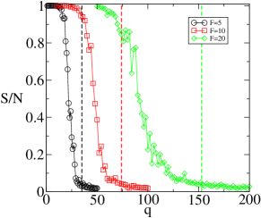
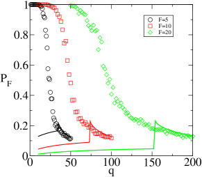
For completeness we re-iterate the behaviour of the baseline Axelrod model ($\theta=\gamma=\delta=0$) in Fig. 1. For any given number $F>2$ of features a discontinuous transition between an ordered state at $q<q_{c}(F)$ and a disordered phase at larger values of $q$ is observed. At $q<q_{c}$ the coarsening dynamics of the model persists until a fully ordered state is reached. For any feature $f=1,\dots,F$ all agents then agree on one opinion, i.e. $\sigma_{if}=\sigma_{jf}$ for all $i,j$. In finite systems such a state is reached after a finite time. Fig. 1 depicts the relative size $S/N$ of the largest culturally homogeneous region of spins as a function of $q$. A homogeneous region $R$ is here defined as a subset of the $L\times L$ agents, so that within $R$ all agents agree on all features comment . As seen in the figure, one finds only one region at convergence for $q<q_{c}$, and has $S/N=1$. At values of $q$ larger than $q_{c}(F)$ dynamic arrest occurs before the system can reach a fully ordered phase. After the arrest no further ordering is possible due to the kinetic constraints imposed on the otherwise attractive spin-dynamics. The system remains in a disordered state, marked by a large number of small cultural regions and a vanishing number of active bonds. $S/N$ remains small at convergence in this regime. As seen in Fig. 1 the fraction $P_{F}$ of fully saturated bonds behaves similarly to $S/N$ at convergence, and can be well captured by the Master equation in the disordered regime. The ordering at low values of $q$ can not be obtained from an approach based on the Master equation Castellano .

Figure 1: (Colour on-line) Relative size $S/N$ of the largest cultural region in the standard Axelrod model with $F$ nominal features, initial conditions drawn from $\sigma_{if}\in\{1,\dots,q\}$ with flat distribution. Symbols show data from simulations run until convergence, system size $N=400$, averaged over $10$ samples, $F=5,10,20$. The vertical dashed lines mark the location of the phase transition as predicted by a numerical integration of the Master equation. The right panel shows $P_{F}$ from simulations (symbols) compared to results predicted by the Master equation (solid lines).

IV.2 Effects of interaction threshold

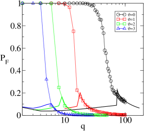
We now turn to the noise-free model with general interaction threshold $\vartheta$. As shown in Fig. 2 the qualitative behaviour of the model is not affected by the introduction of a confidence threshold. As before an ordered phase is found at low values of $q$, and a disordered one at $q$ larger than some critical value $q_{c}(\vartheta,F)$. One finds that an increased confidence threshold suppresses interaction and hence reduces the range of $q$ in which order can be reached. $q_{c}$ is a decreasing function of $\vartheta$ at fixed $F$. Fig. 2 also demonstrates that the Master equation given above describes the qualitative behaviour of the system and dependence on the interaction threshold appropriately. In the disordered phase even a reasonable quantitative agreement between numerical measurements of the fraction of fully saturated bonds and the corresponding theoretical predictions can be observed. We attribute remaining discrepancies to the mean field approximation, inaccuracies in capturing the $2$-dimensional geometry and to finite-size effects.

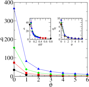
Fig. 3 depicts the phase diagram of the model in the $(\vartheta,q)$ plane for different values of $F$, as obtained from the Master equation pgnum . The disordered phase is found at large values of $\vartheta$ and $q$ respectively, order is reached at low $q$ and/or $\vartheta$. It may here be interesting to ask whether the relevant variable is the absolute interaction threshold $\vartheta\in\{0,\dots,F\}$, or the relative one $\vartheta/F$. In Flache1 ; Flache2 results are for example reported in terms of relative thresholds. The left inset of Fig. 3 confirms that the phase boundaries for different values of $F$ as shown in the main panel do indeed show a reasonable collapse if plotted as a function of $\vartheta/F$. At small values of $\vartheta$ systematic deviations are however observed. A different rescaling was suggested in Maxi2 , where results for the one-dimensional Axelrod model where shown to depend mostly on $q/F$. As demonstrated in the right inset of Fig. 3 equally good collapse is observed in the $(\vartheta/F,q)$ plane, so that we can here not reach a definitive conclusion as to whether there are any independent scaling parameters, and if so which ones they are comment2 .

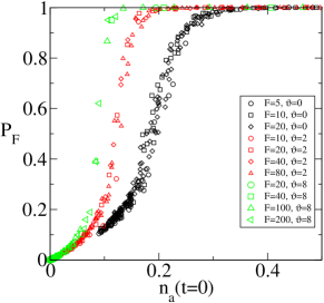
Some indications regarding the relevance of absolute as opposed to relative thresholds can be found in Fig. 4, where we show the density of fully saturated bonds $P_{F}$ as a function of the density of initially active bonds $n_{a}(0)=\sum_{k=\vartheta+1}^{F-1}P_{k}(t=0)$. Simulations are here performed by fixing $\vartheta$ and $F$ and by subsequently varying $q$. $n_{a}(0)$ then decreases with increasing $q$. The data shown in the figure suggest a potential collapse on three different curves, one for each of the tested values $\vartheta=0,2,8$. While these findings might indicate some potential universality as $F$ and $q$ are varied at fixed $\vartheta$, reaching a final conclusion as to whether absolute or relative thresholds are the relevant ones still remains an open question.

Figure 2: (Colour on-line) Fraction of fully saturated bonds $P_{F}$ in the Axelrod model with $F=10$ nominal features and with confidence threshold $\vartheta=3,2,1,0$ (from left to right), initial conditions drawn from $\sigma_{if}\in\{1,\dots,q\}$ with flat distribution. Connected markers are from simulations with $N=400$ agents, run until convergence, averaged over $10$ samples. Thick solid lines show theoretical predictions by the Master equation.

Figure 3: (Colour on-line) Phase diagram of the model with general confidence threshold in the mean-field approximation. Locations of the transitions are obtained from the Master equation. The curves show $F=40,20,10,5$ from top to bottom. The system is in the disordered phase above the respective lines. Ordered states can be expected below. The insets show a rescaling in terms of the relative threshold $\vartheta/F$ (left) and of the relative number of opinion states per feature $q/F$ (right).

Figure 4: (Colour on-line) $P_{F}$ versus fraction of active links $n_{a}(0)$ in initial configuration for nominal Axelrod dynamics at different $\vartheta$ and $F$. Data are from simulations (system size $N=20\times 20$, run until convergence, averages over $10$ samples are taken).

IV.3 Effects of external noise

We now turn to a discussion of the effects of noise on nominal Axelrod dynamics. We will first focus on external noise as introduced above. This type of stochasticity describes random fluctuations which are triggered by an external event, and which result in individual spin components being flipped randomly at a given rate. External noise was introduced in the context of the Axelrod model in Klemmnoise , and the resulting random mutations describe what Axelrod refers to as ‘cultural drift’ Axelrod in the population of agents. Klemm et al. Klemmnoise have studied the effects of external noise as a function of the noise rate and system size in fully equilibrated systems. We here extend this analysis, and consider different cases according to whether the thermodynamic limit or long-time limit is taken first. Results from an integration of the Master equation are discussed in order to provide a semi-analytical description of the system in the limit of infinite size.

IV.3.1 Finite system, equilibrated dynamics

In finite systems a continuous transition between an ordered state at low noise rates $\gamma$ and a disordered state at large $\gamma$ has been identified in Klemmnoise . This transition relates to a characteristic relaxation time $T={\cal O}(N\log N)$ in finite systems. When the noise rate is sufficiently large (larger than $T^{-1}$) stochastic perturbations build up in time, and lead to a disordered state. For $\gamma T<<1$ the system drifts from one ordered state to another in time, time-averaging effectively yields global order. Since at $q>q_{c}$ disorder is observed in the absence of noise ($\gamma=0$), the behaviour of the model in the limit $\gamma\to 0^{+}$ is discontinuous at $q>q_{c}$. As discussed in the next point the finiteness of the system is crucial here, so that the described behaviour cannot be captured by the Master equation.

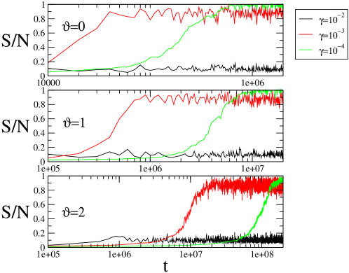
The effects of external noise on finite Axelrod systems with general threshold is depicted in Fig. 5. The behaviour of the model with confidence threshold is here found to be very similar to the one identified in Klemmnoise for conventional Axelrod dynamics. We here focus on $F=10$, $q=100$ as an example, but similar behaviour can be expected for other model parameters in the disordered phase of the noise-free model. For small values of $\gamma$ the system orders after an initial transient. At large magnitude of the applied noise, no ordering is found, consistently with the results of Klemmnoise . This general qualitative picture appears to be independent of the applied threshold. The duration of the equilibration period in cases where the system orders, however, shows a significant dependence on the noise strength and on the chosen threshold. Generally, the time required to reach equilibration increases as $\gamma$ is lowered or as $\vartheta$ is increased, see Fig. 5. The value of $S/N$ at equilibrium is a decreasing function of $\gamma$. In the examples of Fig. 5 equilibration to a value of $S/N\approx 0.1$ occurs fast at $\gamma=10^{-2}$. At lower noise rates, $S/N$ reaches values in the range of $0.8$ to $1$, but only after a substantial equilibration period, which increases as $\gamma$ is lowered. Only models with low or moderate threshold and/or sufficiently large noise strength can hence be equilibrated in reasonable computing time. While analogy suggests that an ordered phase sets also at higher thresholds $\vartheta$ and small enough noise strengths if the dynamics is run long enough, we have not been able to confirm this explicitly due to computational limitations. Approaches based on continuous-time Monte Carlo methods might here potentially be more appropriate than direct simulation of the Axelrod dynamics newman .

Figure 5: (Colour on-line) $S/N$ versus time for $F=10,q=100$. $\vartheta=0,1,2$ in top, middle and lower panel. Curves shown for $\gamma=10^{-2},10^{-3},10^{-4}$ (bottom to top at large times). From simulations, $N=10\times 10$, averages over $10$ runs. The $x$-axes show time in multiples of $N$ microscopic updates, i.e. after $t$ every agent has on average been selected $t$-times for potential update.

IV.3.2 Thermodynamic limit for equilibrated systems

Due to the divergence of the relaxation time $T$ with $N$, the transition just discussed disappears in infinite systems. If, at $q>q_{c}$, the system size is taken to infinity after equilibration, i.e. if equilibrated systems are considered at increasing $N$ while keeping all other parameters fixed, the population always ends up in a disordered state for all $\gamma\geq 0$, as demonstrated in Klemmnoise . The discontinuity at $\gamma\to 0^{+}$ is removed. Equilibrated systems of infinite size cannot be captured by the Master equation, as the latter implies the thermodynamic limit to have been taken first.

IV.3.3 Thermodynamic limit at finite $t$

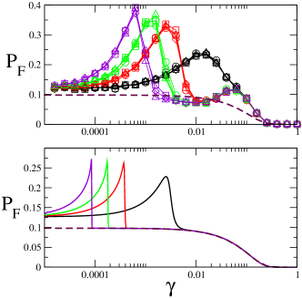
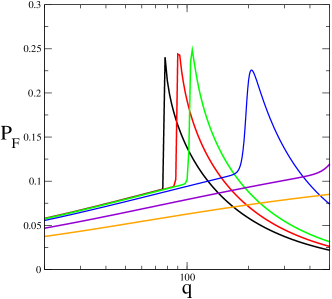
Taking the thermodynamic limit $N\to\infty$ at a fixed number of macroscopic time steps $t$ results in non-trivial behaviour. As displayed in Fig. 6 one finds a disordered state with $P_{F}\approx 0$ at sufficiently large $\gamma$. Partial ordering sets in as $\gamma$ is lowered, with non-monotonous behaviour and a peak of $P_{F}$ at intermediate noise-strengths. As $\gamma$ is reduced further, $P_{F}$ takes small but non-zero values, mostly independent of the noise strength, provided the latter is small enough. Integration of the Master equation confirms this behaviour qualitatively. The non-monotonic behaviour of $P_{F}$ as a function of $\gamma$ at fixed time-scale $t$ is here potentially related to the non-monotonic temporal behaviour of the Axelrod system as observed for example in Castellano ; Redner . Under suitable conditions order parameters such as $P_{F}(t)$ or $S(t)/N$ might become non-monotonic functions of time at fixed values of $q,F,\gamma$. These non-monotonicities are then reflected as peaks in $P_{F}$ when other cuts through parameter space are considered, as in Fig. 6 where $\{t,F,q\}$ are fixed and $\gamma$ is varied, or in Fig. 7 where $q$ is varied at fixed $\{F,t,\gamma\}$.

IV.3.4 Large time limit after taking thermodynamic limit

As the time-scale on which the systems is studied is increased, the peak in $P_{F}$ appears to move further to the left in Fig. 6, i.e. to smaller values of the noise strength $\gamma$. Hence for any fixed $\gamma_{0}$ there is a time-scale $t(\gamma_{0})$ so that $P(F)$ is monotonically decreasing as a function of $\gamma>\gamma_{0}$ on this time-scale. The system is hence disordered at large $\gamma$, and partially ordered at low $\gamma$. This behaviour can successfully be described by the Master equation.

Figure 6: (Colour on-line) $P_{F}$ versus $\gamma$ in a nominal Axelrod system, $F=10,q=100$. Upper panel: results from simulations, run for $t$ macroscopic time-steps, where $t=20000,10000,5000,1000$ from left to right. Circles are for $N=20\times 20$, squares for $N=30\times 30$, diamonds $N=40\times 40$, triangle $N=50\times 50$. Data are averages over $10$ samples. Lower panel: $P_{F}$ from numerical integration of the Master equation, $t=20000,10000,5000,1000$ as above. An Euler-forward scheme with time-step $dt=0.1$ is here used. Dashed line in both panels marks result from Master equation after even longer times ($t=2\cdot 10^{5}$).

Figure 7: (Colour on-line) $P(F)$ versus $q$ in a nominal Axelrod system, $F=10$. Results are from numerical integration of the Master equation up to $t=5000$. Curves show $\gamma=0.0001,0.0005,0.001,0.005,0.025,0.05$ from left to right at the maximum. Curves for $\gamma=0.025$ and $\gamma=0.05$ still display a maximum, but to the right of the plotted range of $q$.

IV.4 Effects of interaction noise

We next turn to a discussion of the effects of interaction noise, as parametrised by its amplitude $\delta$. This type of stochasticity facilitates interaction, as it removes kinetic constraints and allows agents sharing $\vartheta$ or less opinions to interact (at rate $\delta$), while in standard Axelrod dynamics they would not be able to align spin components. While the external noise of amplitude $\gamma$ has an ambiguous role of inducing order at low amplitudes and of driving the system to disorder at large $\gamma$, interaction noise can generally be expected to favour order. It his hence interesting to study the system in presence of both types of randomness, and to identify re-inforced ordering behaviour or (at small $\gamma$) potential competition between the ordering and disordering stochasticity (at large $\gamma$)

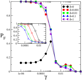
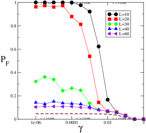
Results for a nominal Axelrod system with both types of noise are reported in Fig. 8. The data indicate that the effects of interaction noise are mostly to facilitate order for large ranges of fixed external noise $\gamma$. More specifically, the effects of interaction noise is to reduce the time-scale on which finite systems order in the presence of external noise. The left panel of Fig. 8 shows the concentration $P_{F}$ of bonds with full overlap in an Axelrod system run for a time which is not long enough for the system without interaction noise (circles, $\delta=0$) to develop order at the studied magnitudes $\gamma$. Order at $\gamma\lesssim 0.001$ would develop only if the system were run for longer times, and had fully equilibrated. The curves for non-vanishing amplitude $\delta$ demonstrate the effect of interaction noise, the system now orders at small noise strengths $\gamma$ . While the qualitative behaviour of the equilibrated system is not altered, the facilitation of the kinetic constraints drastically reduces equilibration times, and the system orders at sufficiently low $\gamma$ even after moderate running times. Interestingly the noise strength $\gamma_{0}$ separating the ordered from the disordered regime of the fully equilibrated system appears not to be affected much by the interaction noise. The curves displayed in the left panel of Fig. 8 are indeed mostly independent of $\delta$, as long as $\delta>0$. It might potentially be interesting to study even lower $\delta$, although probably unrealistic from the sociological point of view comment3 .

We conclude that the effect of interaction noise is to reduce relaxation times, but that it does not alter the phase behaviour of the model, with an ordered phase at low $\gamma$, and a disordered one at large $\gamma$. As in the absence of interaction noise ($\delta=0$) this transition is present only in finite systems, seen in the inset of the left panel of Fig. 8 and in the right panel. As the system size is increased at equilibrium the order-disorder crossover moves to smaller values of the noise strength $\gamma$, and can be expected to be absent in the thermodynamic limit, where only the disordered region prevails. Indeed rescaling of the data in the inset of the left panel demonstrates that $\gamma N\ln N$ is the relevant scaling variable, similar to the observations of Klemmnoise . At finite running times $t$ the order at low $\gamma$ is gradually reduced with increased system size and in the thermodynamic limit the system is qualitatively well described by the Master equation.

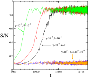
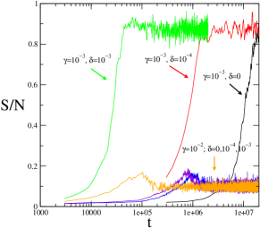
Fig. 9 finally confirms that this behaviour is not limited to the standard Axelrod dynamics with vanishing interaction threshold ($\vartheta=0$). Interaction noise reduces the time-scale on which the system orders at small $\gamma$ also in the model with moderate non-zero thresholds, and that the system at $\vartheta>0$ behaves very much like the one at $\vartheta=0$.

Figure 8: (Colour on-line) Effects of interaction noise. Left: $P_{F}$ versus $\gamma$ for Axelrod model ($F=10,q=100,\vartheta=0$), $N=20\times 20$, run for $20000$ steps (averages over $10-20$ samples) The inset shows results for systems of size $N=10\times 10,20\times 20,40\times 40,60\times 60$ at $\delta=0.1$ from right to left. Right: $P_{F}$ for different system sizes at fixed $\delta=0.1$ at $t=5000$. Dashed line in right panel is from numerical integration of the Master equation.

Figure 9: (Colour on-line) Effects of interaction noise. $S/N$ versus time $t$ at different levels of external and interaction noise. Data is from simulations of systems with $N=10\times 10$ agents. The left part shows $\vartheta=0$ (averages over $50$ samples), the right one $\vartheta=2$ ($10$ runs, data smoothened by running averages). $F=10,q=100$ in both panels. At large $\gamma$ no order is reached, independently of $\delta$. For small enough $\gamma$ the system orders, the time-scale on which this occurs is largely reduced by the introduction of interaction noise, and increases as the interaction threshold is raised (note the different scaling on the time axes on the left and right).

V Euclidean Axelrod dynamics

We now turn to a modification of the Axelrod dynamics in which a metric allowing for gradual notions of agreement between agents is introduced. As before, opinions take discrete values $\sigma_{if}\in\{1,\dots,q\}$. However, the ‘distance’ between two spins $\vec{\sigma}_{i}$ and $\vec{\sigma}_{j}$ is no longer measured in terms of the number of features on which the corresponding agents agree, but based on the following Euclidean distance between the spin-vectors $\vec{\sigma}_{i}$ and $\vec{\sigma}_{j}$:

$$d=\sqrt{\frac{1}{F(q-1)^{2}}\sum_{f=1}^{F}(\sigma_{if}-\sigma_{jf})^{2}}.$$ (3)

Thus the distance between two agents ranges between $0$ and $1$. It takes the maximal value $d=1$ if and only if the opinions of the two agents are diametrically opposed, i.e of for any feature $f$ one has $\sigma_{if}=1,\sigma_{jf}=q$ or $\sigma_{if}=q,\sigma_{jf}=1$. Distances different from zero or one thus indicate partial agreement between the two agents.

In the following we will take the potential of two neighbouring agents to interact to be given by the following logit-rule logit :

$$p(d)=\frac{1}{1+e^{\beta(d-d_{0})}}.$$ (4)

$\beta$ is a control parameter allowing for the introduction of interaction noise. The case $\beta=\infty$ here corresponds to the noise-free (zero temperature) case. If $\beta=\infty$, agents with distance $d>d_{0}$ are unable to interact, $p(d>d_{0})=0$, whereas interaction always occurs for pairs of agents with distance $d<d_{0}$. $d_{0}$ is thus a threshold parameter, with large $d_{0}$ corresponding to a regime of strong confidence of agents in other people’s opinions, and small $d_{0}$ to cases in which interaction is rare. In order to avoid confusion let us at this point stress that the role of the threshold $d_{0}$ is inverse to the one of $\vartheta$ in the nominal Axelrod model: large $\vartheta$ make interaction rare, whereas large $d_{0}$ facilitate spin updates.

Choosing finite values of $\beta$ turns the hard threshold into a soft one. Interaction rates decrease smoothly with increasing distance. Crucially, at finite $\beta$, interaction is always possible in principle, even if $d>d_{0}$. For $\beta=0$ finally, interaction is fully stochastic and independent of $d$. At any iteration, any chosen pair of neighbouring agents interacts with probability $1/2$.

Let us summarise the resulting dynamics:

1. Select one spin $i\in\{1,\dots,N\}$ at random. Subsequently select one of its four nearest neighbours at random. Call this second spin $j$.

2. Compute the Euclidean distance $d(i,j)$ between $i$ and $j$.

3. If $d(i,j)=0$ both agents agree on all features. Interaction has no effect. If $d\equiv d(i,j)>0$ then with probability $p(d)$ as defined above spins $i$ and $j$ interact as in the nominal Axelrod model: one feature $f$ is chosen at random so that $\sigma_{if}\neq\sigma_{jf}$. Then set $\sigma_{if}=\sigma_{jf}$.

4. External noise. With probability $\gamma$ perform the following: choose one spin $i$ and one feature $f$ at random. Set $\sigma_{if}$ to a value chosen randomly from $\{1,\dots,q\}$.

5. Resume at (i).

V.1 Noise-free dynamics

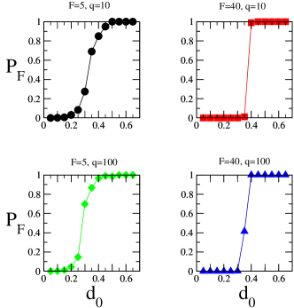
The behaviour of the noise-free system with Euclidean metric is described in Fig. 10. A transition between a disordered phase at low thresholds $d_{0}$ and an ordered state at larger values of $d_{0}$ is observed. The behaviour in these two phases is as follows: at low $d_{0}$ only neighbouring agents with small differences in opinion can interact, so that the fraction of active bonds initially contained in the system is small. Dynamic arrest occurs quickly, and the system remains disordered. At large enough thresholds $d_{0}$ the coarsening dynamics can persist until a fully ordered state is reached. Interestingly, as shown in Fig. 10, the critical value of the threshold $d_{0c}$ does not depend much on the choice of $F$ and $q$, and takes values $d_{0c}\approx 0.4$. The transition appears to become sharper at larger values of $F$ (see Fig. 10).

Plotting $P_{F}$ versus $q$ at fixed $F$ suggests that $q$ plays no significant role in the Euclidean model. Only for small values of $q$ can a dependence of $P_{F}$ on $q$ be detected. This invariance is intuitively to be expected as $d$ is normalised to range between $0$ and $1$ in the setup chosen here, so that $q$ is merely a measure for how many discrete values can occur inbetween. Simulations with continuous opinions ranging in the interval $[0,1]$ (not shown here) reveal a behaviour very similar to the one depicted in Fig. 10. We have also tested models with continuous opinions, in which both interacting agents agree on the average opinion of a given feature in case of interaction (with the same metric and kinetic constraints as before), and find similar behaviour as a function of $d_{0}$. Similar models are discussed in Redner2 ; Redner3 , mostly focussing on the case of one feature.

Figure 10: (Colour on-line) $P_{F}$ versus interaction threshold $d_{0}$ for the Euclidean model. Data is from simulations at different values of $F$ and $q$ ($N=20\times 20$, averaged over $10$ samples). Simulations are run until each bond has distance $d=0$ or $d>d_{0}$, i.e. until no active bonds are left in the system.

V.2 Effects of external and interaction noise

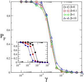
The behaviour of the Euclidean system under the influence of external and interaction noise is shown in Fig. 11. As seen in the main panel, a crossover between an ordered regime at low magnitudes $\gamma$ of the external noise and a disordered state at higher noise-amplitudes is found, very much like in the nominal Axelrod model. Interaction noise (finite $\beta$) appears to have only little effect on this crossover for all values tested. Due to long equilibration times we have not performed a full analysis of the impact of external noise ($\gamma>0$) in the large-$N$ limit of the model zero-temperature ($\beta=\infty$). The inset of Fig. 11 however demonstrates that at finite $\beta$ the range of $\gamma$ in which the system orders is reduced as the system size is increased, similarly to what is found in the nominal Axelrod model. The ordering behaviour at small values of the external noise strength hence again appears to be present only in finite systems.

Figure 11: (Colour on-line) Effects of noise on the Euclidean model. Main panel shows $P_{F}$ versus $\gamma$ from simulations of a system of size $N=20\times 20$, run for $200000$ macroscopic steps, averages over $10$ samples ($F=10,q=100$). The interaction threshold is $d_{0}=0.3$, i.e. the system is in the disordered phase if $\beta=\infty$. Inset: $P_{F}$ versus $\gamma$ at fixed $\beta=1$ for system sizes $N=40^{2},20^{2},10^{2}$ from left to right (same simulation parameters as in main panel, $5$ samples only for $N=40^{2}$).

V.3 Extremism and polarisation

One particular potential application of metric Axelrod models is to study extremism, and the effects of a small number of highly polarised agents, e.g. with opinions at the extreme ends of the political spectrum. Having studied the effects of uniform confidence thresholds on the opinion dynamics, we here extend the model to the case of heterogeneous, i.e. agent-specific thresholds. Here any agent $i\in\{1,\dots,N\}$ holds an individual threshold $d_{0,i}$. In an interaction with a neighouring agent $j$ he adjusts his opinion vector $\sigma_{i}$ only if $d(i,j)<d_{i}$, i.e. $d_{0}$ in Eq. (4) is replaced by $d_{0,i}$. Agents with large $d_{0,i}$ are thus likely to interact with others, and have a large tolerance against opinions in their surroundings. Agents who are unlikely to modify their own opinion vector are described by small interaction thresholds. Related work on other opinion dynamics models, mostly with continuous opinions and focusing on one feature or on nominal features, can be found in Weisbuch1 ; Weisbuch1a ; Weisbuch2 ; Fanelli , see however also Stauffer . Our simulations here focus on the effects of extremists in the context of a multi-variate opinion dynamics model ($F>1$) with discrete opinions and metric features.

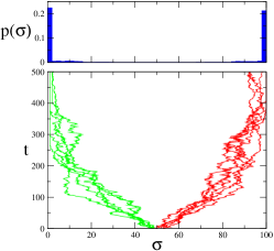
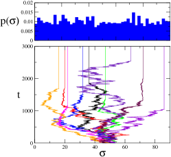
In this section we assume that the population of agents contains a fraction $\varepsilon$ of what we will call extremists. These are agents whose opinion vectors take extreme values $\sigma_{if}=1$ or $\sigma_{if}=q$ at the beginning of the dynamics, and who are intolerant against other agents’ opinion. In particular we assume an interaction threshold small $d_{e}$ for such agents. All other agents are taken to have a uniform threshold $d_{0}$ as before and are initialised at random opinion vectors. The choices in the simulations presented in Fig. 12 are $\varepsilon=0.05$, $d_{e}=0.05$ and $d_{0}=0.6$ (the latter threshold is chosen to ensure the system is in the ‘active’ ordered phase where dynamics persists long enough to prevent the system from remaining stuck in a configuration similar to the initial condition). The figure shows the time evolution of the average opinion of the population on a given feature, along with the distribution of opinions at convergence. Apart from the initial conditions no stochasticity is present in the simulations shown in Fig. 12, i.e. we have $\beta=\infty$, $\delta=0$. As shown in the left panel a small group of extremists can polarise the population, provided they are inert enough against adapting their own opinions. The figure shows $10$ runs of the Axelrod dynamics. In each run extremists are chosen either to correspond to opinion states $1$ or $q$. Extensions to two groups of extremists at either end of the political spectrum, or to cases in which extremists have polarised opinions only on some but not all features, are straightforward. The right panel shows the behaviour of the system in absence of extremists. Here the average opinion on each feature converges to a random value between $1$ and $q$ depending on the stochastic initial conditions, and the resulting histogram of final opinions is flat.

Figure 12: (Colour on-line) Metric model with (left) and without extremists (right). In the left panel a fraction of $\varepsilon=0.05$ of extremists was used, with $d_{e}=0.05$. $d_{0}=0.6$ as well as $F=10,q=100$ in both panels. Each panel shows the average opinion $N^{-1}\sum_{i}\sigma_{if}$ on a given feature $f$ as function of time for $10$ individual runs of a system with $N=20\times 20$ individuals, started from random initial conditions. Histograms of opinions at convergence are shown in the top part (data for $200$ samples and from all $F$ features used to generate histograms). .

VI Summary and conclusions

We have extended Axelrod model for social influence to include varying interaction threshold, noise and metric features. In the basic model, which is two-dimensional, individuals are represented as multi-component spins and interact to become culturally closer, starting from a disordered random initial state. In our extensions some external and interaction noises are introduced, a confidence threshold limits the interaction, and a notion of distance between opinion is considered. We find that the confidence threshold does not influence the qualitative behaviour of the model, and that the typical transition, separating an ordered and a disordered equilibrium state, is preserved and determined basically by the initial probability of interaction between two individuals. The threshold limits the probability of interaction, and hence favors disorder. The introduction of an external noise brings in finite systems a continuous transition between an order-favoring and a disorder-favoring role of the noise, according to whether the noise is small or large respectively, independently of the threshold. This implies a discontinuity, in the region where the final state would be disordered in the absence of external noise. Such a discontinuity is removed in the thermodynamic limit. An interaction noise instead always favors order by reducing relaxation times, and does not alter the phase structure of the model. The other variant we study is the one with a notion of distance between opinions. We find that the model exhibits an order-disorder transition as the distance threshold is varied, consistently with the idea that the transition is the result of the competition between an ordering dynamics (the relative importance of which is determined by the distance threshold) and an initial disorder (as measured by size of the space from which the starting configuration is drawn at random). Moreover, the introduction of heterogeneous confidence thresholds in the context of metric Axelrod systems allows one to study e.g. the question of whether extremism can prevail in such models. We find that the presence of a small fraction of individuals with a sufficiently rooted opinion can drive the whole population to the extreme ends of the opinion spectrum. Further application of heterogeneous interaction thresholds and metric features might include extensions addressing immigration or geographic barriers. Immigrants can for example be assumed to be more likely to interact with other immigrants than with members of the original population, and geographical barriers can be modelled by suppressing interaction at certain locations in space. This would lead to different interaction thresholds and tolerance levels, modulated either in space or dependent on the two agents picked for potential interaction.