X-ray scattering from stepped and kinked surfaces: an approach with the paracrystal model

Abstract

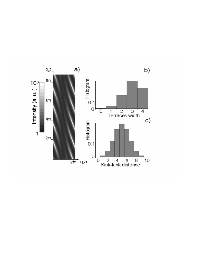
A general formalism of X-ray scattering from different kinds of surface morphologies is described. Based on a description of the surface morphology at the atomic scale through the use of the paracrystal model and discrete distributions of distances, the scattered intensity by non-periodic surfaces is calculated over the whole reciprocal space. In one dimension, the scattered intensity by a vicinal surface, the two-level model, the N-level model, the faceted surface and the rough surface are addressed. In two dimensions, the previous results are generalized to the kinked vicinal surface, the two-level vicinal surface and the step meandering on a vicinal surface. The concept of Crystal Truncation Rod is generalized considering also the truncation of a terrace by a step (yielding a Terrace Truncation Rod) and a step by a kink (yielding a Step Truncation Rod).

I Introduction

The control of the morphology and structure of surfaces is one key point to elaborate high quality devices, since defects such as steps, kinks or more generally surface roughness may drastically influence their physical properties. Defects may also be used to promote catalytic reactions or as preferential nucleation sites for the self-assembling of nanostructures Brune et al. (1998); Leroy et al. (2005), e. g. in view of ultra-high density recording. In this context, the development of surface characterization tools is highly appreciated. If scanning probe microscopy is the technique of choice to get local real space information, statistical averages and in situ experiments are advantageously performed with diffraction techniques. Numerous real time studies of thin films growth, coarsening or roughening have been performed, for instance with X-ray Renaud et al. (2003); Braun et al. (2004); Renaud et al. (1992), Spot Profile Analysis Low Energy Electron Diffraction (SPA-LEED) Tegenkamp et al. (2002); Sotto and Croset (2000), Helium Atom Scattering (HAS) Farias and Rieder ; Crottini et al. (1997); Ernst et al. (1992) or Reflection High Energy Electron Diffraction (RHEED) Dulot et al. (2003) techniques.
In particular X-ray scattering have the advantage over the other techniques of a weak scattering cross section which makes possible the quantitative analysis of the diffraction patterns in the framework of the kinematic approximation. The purpose of this paper is to revisit the scattering theory by disordered stepped and kinked surfaces in the context of the development of grazing incidence X-ray studies in surface science. It extends elder works which essentially dealt with Helium and electron diffraction.

The main problem in the calculation of the diffraction by disordered surfaces is to have a statistical description of the morphology and to be able to calculate the scattered intensity. If the morphology is perfectly periodic, the scattered intensity is calculated in a straightforward way. The structure factor of the unit cell which repeats from the surface to the bulk, i.e. the Fourier transform of its electronic density, has to be evaluated. Then the scattered intensity is the modulus square of the sum of the amplitude scattered by all the unit cells. In the special case of surface diffraction, a semi-infinite sum has to be done in the direction perpendicular to the surface. If one considers the simple case of a cubic lattice, the intensity reads:

$$I(q_{x},q_{y},q_{z}) = \mid\widetilde{F}_{cell}(q_{x},q_{y},q_{z})\mid^{2}\sum_{n_{1}=-\infty}^{+\infty}\sum_{n_{2}=-\infty}^{+\infty}\sum_{n_{3}=0}^{+\infty}e^{in_{1}q_{x}a}e^{in_{2}q_{y}b}e^{in_{3}q_{z}c}$$ (1)

$$= \frac{\mid\widetilde{F}_{cell}(q_{x},q_{y},q_{z})\mid^{2}}{(2\sin(q_{z}c/2))^{2}}\sum_{n_{1}=-\infty}^{+\infty}\sum_{n_{2}=-\infty}^{+\infty}\delta\left(q_{x}-n_{1}\frac{2\pi}{a}\right)\delta\left(q_{y}-n_{2}\frac{2\pi}{b}\right)$$

Where $a$, $b$ and $c$ are the lattice parameters along the coordinates $x$, $y$ and $z$. $q_{x}$, $q_{y}$ and $q_{z}$ are the reciprocal space coordinates and $\delta$ is the Dirac distribution.

This well known result tells us that the intensity is not zero in between Bragg peaks in the direction perpendicular to the surface. Such scattering rods are called Crystal Truncation Rods (CTR) Robinson (1986) and arise because the crystal is truncated. However, in general, the surface morphology deviates from this ideal perfectly ordered case. The introduction of disorder may lead to significant changes of the scattered intensity, particularly in anti-Bragg condition where the intensity is proportional of that scattered by half a lattice plane, and to an increase of calculation complexity. It is necessary to consider the scattered intensity by objects for which sizes and distances from one to another are correlated. For instance in the case of a vicinal surface, the distance separating two nearest neighbor terraces from their respective centers is completely determined by their widths. Therefore it is impossible to describe the scattered intensity as the multiplication of the square modulus of the form factor of the terrace width (averaged over the widths distribution) by an interference function. Several authors have addressed this problem and some analytical results have been obtained assuming generic distributions of terrace widths Houston and Park (1971); Lent and Cohen (1984); Pukite et al. (1985); Croset and de Beauvais (1997); Uimin and Lindgård (1997); Wollschläger (1997). We propose here a method based on the paracrystal model Hosemann and Bagchi (1962); Guinier and Fournet (1955); Welberry (1985) and an appropriate choice of the elementary scattering object at the atomic scale to evaluate the scattered intensity from stepped or kinked surfaces. Previous results of HAS and electron diffraction, i.e. the two-level model, the N-level model, the vicinal surface and the randomly stepped surface are extended to X-ray scattering. In comparison with these elder results the contribution of deep layers gives rise to a CTR prefactor. This one-dimensional approach is further expanded to two dimensions for some specific surface morphologies. All calculations are performed assuming the atomic structure of matter (discrete values of the terrace size and the kink-kink distance) which allows evaluating the scattered intensity in the whole reciprocal space and not only around Bragg peaks. This point is of importance since surface structure characterization is usually performed measuring the CTR or during growth by measuring the scattered intensity in anti-Bragg conditions. Therefore Small and Wide-Angle scattering data may be analyzed with the same model. The concept of CTR is extended to the truncation of a terrace by a step (Terrace Truncation Rod) and to the truncation of a step edge by a kink (Step Truncation Rod) thanks to the terrace-step-kink model used for the description of the surface morphology.

This paper is organized as follow. The method is first presented for a classical one-dimensional analysis of surfaces. Different surface morphologies are successively treated: (i) the vicinal surface, (ii) the two-level model, (iii) the N-level model and (iv) the randomly stepped surface ($\infty$-level model), illustrating the choice of the elementary scattering object as well as that of paracrystals. The cases of faceted surfaces are next treated, demonstrating the generality of the formalism. Follows a generalization to two-dimensions for some specific cases: (i) the kinked vicinal surface, (ii) the two-level vicinal surface and (iii) the $\infty$-level vicinal surface (or step meandering on a vicinal surface). In a last part, a method is briefly proposed to take into account in the calculation the intensity scattered by the elastic distortions induced by periodic steps and kinks below the surface.

II One dimensional analysis of scattering from surfaces

II.1 The vicinal surface

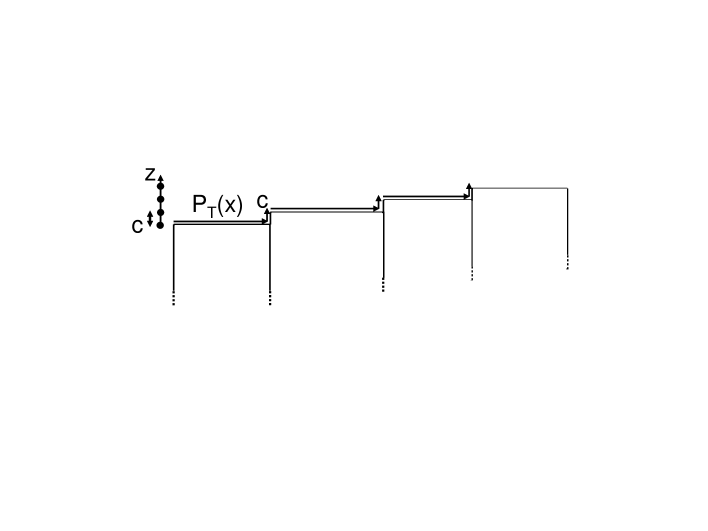
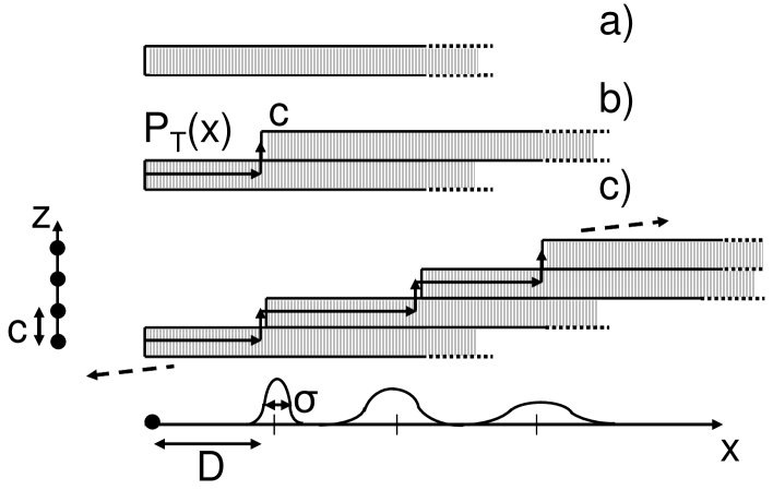
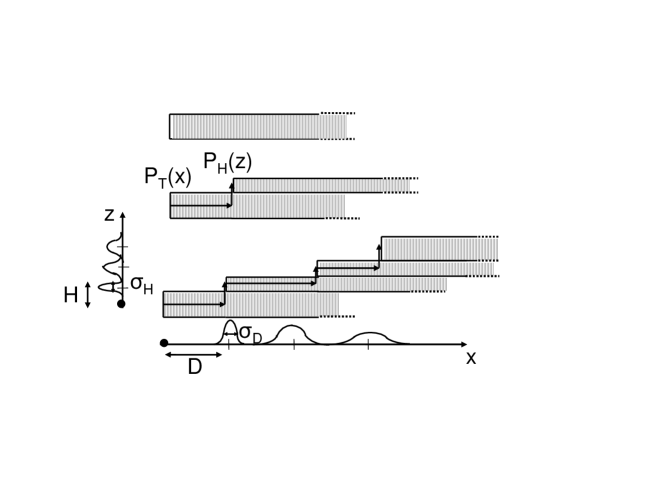
The usual approach for the calculation Pflanz and Moritz ; Croset and de Beauvais (1998) of the X-ray diffraction by a vicinal surface with constant step height is based on a description of the surface as a stacking of terraces along the x-axis (Fig 1). Then the scattered intensity is averaged over all possible configurations of the step positions. Despite its simplicity from a formal point of view, it is necessary to take into account the correlations between the terrace widths and the distances that separate them. However a precise analysis of vicinal surfaces shows that an elementary object without any size distribution can be extracted from the surface morphology. This object consists of a semi-infinite plane parallel to the terraces (along the x-axis), starting at the step edge (Fig 2) and penetrating into the bulk. Concerning the terrace width distribution and the average over all the configurations, the use of the auto-correlation function of the step positions in the framework of the paracrystal model is straightforward. Therefore this method allows separating in a simple way the role played by the step structure from that played by the terrace width distribution. In the framework of this model, the scattered intensity is the product of the square modulus of the form factor of the elementary object $\widetilde{F}_{vicinal}(q_{x},q_{z})$ by an interference function $S(q_{x},q_{z})$.

$$I(q_{x},q_{z})=\mid\widetilde{F}_{vicinal}(q_{x},q_{z})\mid^{2}\times S(q_{x},q_{z})$$ (2)

The form factor of the elementary object is a semi-infinite sum, which yields the usual Crystal Truncation Rod behavior parallel to the terrace width:

$$\widetilde{F}_{vicinal}(q_{x},q_{z}) = \widetilde{F}_{cell}(q_{x},q_{z})\sum_{n=0}^{\infty}e^{inq_{x}a-n\mu a}$$ (3)

$$= \widetilde{F}_{cell}(q_{x},q_{z})\frac{e^{-iq_{x}a/2}}{-2i\sin(q_{x}a/2)}$$

where $\widetilde{F}_{cell}(q_{x},q_{z})$ is the structure factor of the unit cell, $a$ is the lattice parameter along the x axis and $\mu$ is the projected absorption coefficient along the x axis. One must remember that the above formula is not correct near Bragg peaks of perfect crystals due to multiple diffraction effects. The second part of the calculation concerns the interference function, i.e. the Fourier transform of the auto-correlation function of all the step positions. The autocorrelation function, $g(x,z)$, is obtained as an infinite summation over $n$ of the probabilities $P_{n}(x,z)$ of having a $n^{th}$ neighbor step ($A_{n}$) at a distance (x,z) from a step $A_{0}$ arbitrary located at the origin $(P_{0}(x,z)=\delta(x)\times\delta(z))$.

$$g(x,z)=\sum_{n=-\infty}^{\infty}P_{n}(x,z)$$ (4)

To calculate each $P_{n}(x,z)$ term, we assume that the distance between nearest neighbor steps is described by a probability law, the terrace widths distribution $P_{T}(x)$, and that there is no correlation between the sizes of neighboring terraces. Within this assumption, $P_{n}(x,z)$ can be obtained step by step building the vicinal surface. The probability for the first neighbor step $A_{1}$ to be located at the (x,z) coordinate is $P_{1}(x,z)=P_{T}(x)\times\delta(z-c)$, where c is the step height. The probability of having a second neighbor step $A_{2}$ at (x’,z’) results from the multiplication of the probability of having a first neighbor step $A_{1}$ located at (x,z) by the probability of having $A_{2}$ and $A_{1}$ separated by the vector (x’-x,z’-z) integrated over all intermediate $A_{1}$ positions. This probability is simply the convolution product of two probability laws : $P_{1}(x,z)\otimes P_{1}(x,z)=P_{1}(x,z)^{\otimes 2}$. This result can be generalized for the $n^{th}$ neighbor step :

$$P_{n}(x,z)=[P_{1}(x,z)]^{\otimes n}=[P_{T}(x)\times\delta(z-c)]^{\otimes n}$$ (5)

After adding the contribution of steps located on the negative x axis, the interference function is obtained by Fourier transform of the auto-correlation function of the step positions :

$$S(q_{x},q_{z}) = FT\left\{g(x,z)\right\}$$

$$= FT\left\{\delta(x)\times\delta(z)+\sum_{n=1}^{\infty}\left([P_{T}(x)\times\delta(z-c)]^{\otimes^{n}}+[P_{T}(-x)\times\delta(z+c)]^{\otimes^{n}}\right)\right\}$$

$$S(q_{x},q_{z}) = 1+(\widetilde{P}_{T}(q_{x})e^{iq_{z}c}+(\widetilde{P}_{T}(q_{x})e^{iq_{z}c})^{2}...+c.c.)$$ (6)

where $\widetilde{P}_{T}(q_{x})=\int_{-\infty}^{+\infty}P_{T}(x)e^{iq_{x}x}dx$ is the characteristic function of the terrace widths distribution and c.c. is the complex conjugate part resulting from the contribution of steps located on the negative x axis. The geometric summation converges as $\mid\widetilde{P}_{T}(q_{x})\mid<1$ and one gets :

$$S(q_{x},q_{z}) = Re\left\{\frac{1+e^{iq_{z}c}\widetilde{P}_{T}(q_{x})}{1-e^{iq_{z}c}\widetilde{P}_{T}(q_{x})}\right\}$$ (7)

Where $Re$ stands for the real part. Therefore the scattered intensity is :

$$I(q_{x},q_{z}) = \left[\frac{\mid\widetilde{F}_{cell}(q_{x},q_{z})\mid}{2\sin{(q_{x}a/2)}}\right]^{2}Re\left\{\frac{1+e^{iq_{z}c}\widetilde{P}_{T}(q_{x})}{1-e^{iq_{z}c}\widetilde{P}_{T}(q_{x})}\right\}$$ (8)

$$= \left[\frac{\mid\widetilde{F}_{cell}(q_{x},q_{z})\mid}{(2\sin{(q_{x}a/2)}2\sin{(q_{z}c/2)})}\right]^{2}Re\left\{2\frac{(1-e^{iq_{z}c})(1-\widetilde{P}_{T}(q_{x}))}{1-e^{iq_{z}c}\widetilde{P}_{T}(q_{x})}\right\}$$

This expression has been obtained by Pukite et al. (see Eq. 18-19 of Ref Pukite et al. (1985)) or for instance by Rao et al. in the special case of the geometric distribution (see Eq. 16 of Ref Rao and Hibma (1991)). Now an additional prefactor $\frac{1}{2\sin(q_{z}c/2)^{2}}$ (the CTR term) corresponding to the contribution of deep layers has to be included. Moreover the usual prefactor $\frac{1}{q_{z}^{2}}$ is replaced by $\frac{1}{\sin(q_{z}c/2)^{2}}$ to account for the discontinuous structure of the lattice. Equation 8 highlights the symmetric roles played by steps and terraces as $e^{iq_{z}c}$ and $\widetilde{P}_{T}(q_{x})$ are respectively the characteristic functions of the step height and the terrace widths distribution. As shown in Appendix A, this result can be generalized for an arbitrary distribution of step heights $P_{S}(z)$.

$$I(q_{x},q_{z})=\left[\frac{\mid\widetilde{F}_{cell}(q_{x},q_{z})\mid}{(2\sin{(q_{x}a/2)}2\sin{(q_{z}c/2)})}\right]^{2}Re\left\{2\frac{(1-\widetilde{P}_{S}(q_{z}))(1-\widetilde{P}_{T}(q_{x}))}{1-\widetilde{P}_{S}(q_{z})\widetilde{P}_{T}(q_{x})}\right\}$$ (9)

where $\widetilde{P}_{S}(q_{z})$ is the characteristic function of the step height distribution. The pre-factors $\frac{1}{2\sin{(q_{z}c/2)}}$ and $\frac{1}{2\sin{(q_{x}a/2)}}$ can be assigned respectively to the ideal truncation of an infinite crystal by a flat surface, the so called CTR (see Eq. 1), and to the truncation of an infinitely large terrace by a step. In analogy to the CTR terminology, the $\frac{1}{2\sin{(q_{x}a/2)}}$ term can be called Terrace Truncation Rod (TTR). Therefore, there is no intensity extinction at $q_{x}a=(2n+1)\pi$, i.e. in anti-bragg condition perpendicular to the step edges. Going further, a high sensitivity to the step edges roughness is expected by the combination of anti-bragg conditions both in $q_{x}$ and $q_{z}$ directions. This point will be discussed in more details within the two-level vicinal surface model. We have to add however that the scattered intensity may only be measurable for large enough miscut angles as the integrated intensity (i.e. in case of long range order) in these experimental conditions is proportional to the number of atoms located at step edges.

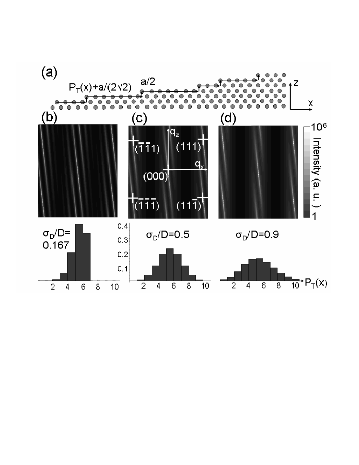
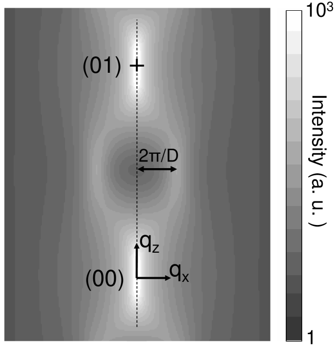
To highlight the result given by Eq. 8, let’s consider the intensity scattered by a vicinal surface $(11n)$ of a fcc crystal (Fig 3). The intensity is calculated in the plane of the reciprocal space perpendicular to the step edge direction ($q_{x}0q_{z}$). The atoms not located on the side view section (at $y\neq 0$) are included into the calculation thanks to the structure factor of the unit cell. Monoatomic steps are assumed with different terrace widths distributions. The distributions are chosen discrete by hypothesis to perform quantitative calculations in the whole reciprocal space (Appendix B). Of course if the atomic resolution is not required continuous distributions are enough. The additional shift in the $x$ direction for adjacent terraces ($\frac{a}{2\sqrt{2}}$) is mandatory to keep the fcc lattice structure. It is taken into account in the calculation adding a phase shift, $e^{iq_{x}\frac{a}{2\sqrt{2}}}$, to the characteristic function of the terrace width distribution. As the FWHM of the terrace size distribution gets larger, the scattering rod gets broader and second and third order satellites disappear in agreement with the increase of disorder. Of course depending on the miscut angle, the scattering rods are more or less tilted as they follow the direction perpendicular to the macroscopic surface plane. This remark is absolutely true close to a Bragg peak, however nonlinear rods may exist in some cases at larger wavevector transfer. For instance it will be shown at the end (Fig 15) that a non integer value of the mean terrace size yields a S shape of the scattering rods.

II.2 The two-level model

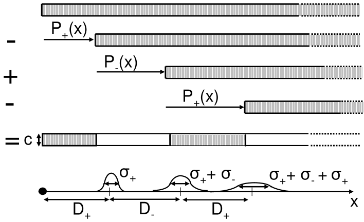
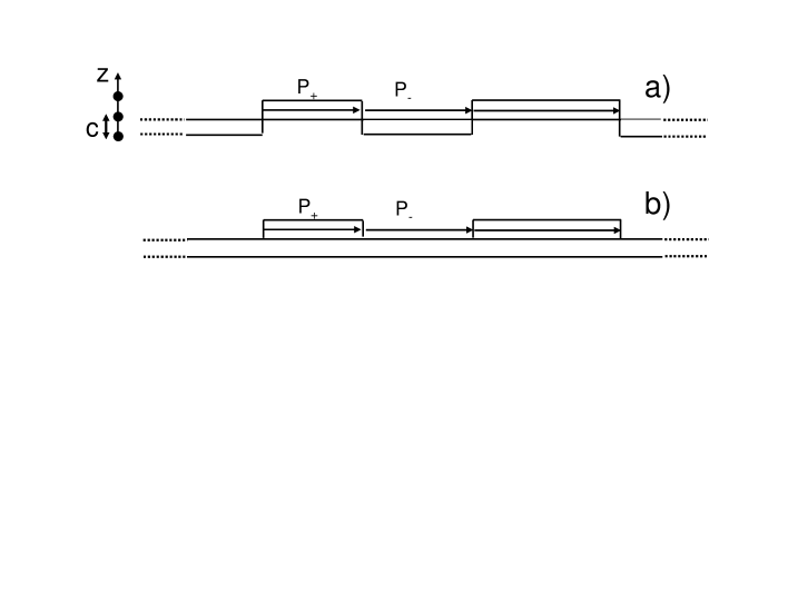
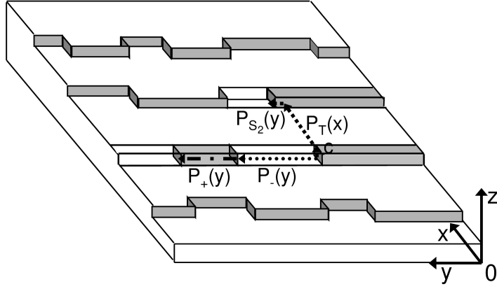
The two-level model has been widely used in the literature to describe the intensity scattered by a surface during the homo-epitaxial growth in the sub-monolayer regime. The two level model allows evaluating the intensity scattered by a surface with a small roughness. The first models developed (e.g. $\beta$ model Robinson (1986); Vlieg et al. (1988)) do not provide any information on the line shape of the diffuse scattering parallel to the surface except a so called correlation length. Improvements have allowed analyzing the line shape assuming a terrace widths distribution Lent and Cohen (1984); Pflanz and Moritz ; Croset and de Beauvais (1997). In this section, we revisit the previous calculations. The two-level model consists in alternating upward and downward steps (Fig 4). As for the vicinal surface, we consider the same elementary object, i.e. a semi-infinite sum of unit cells parallel to the terrace plane. That way we can built step by step a two-level model folding nodes alternatively with this elementary object and its exact opposite (opposite electronic density). Their form factors are opposite of each other and reads:

$$\widetilde{F}_{\pm}(q_{x},q_{z})=\pm\widetilde{F}_{cell}(q_{x},q_{z})\sum_{n=0}^{\infty}e^{inq_{x}a}=\pm\widetilde{F}_{cell}(q_{x},q_{z})\frac{e^{-iq_{x}a/2}}{-2i\sin{(q_{x}a/2)}}$$ (10)

Assuming that $P_{+}(x)$ and $P_{-}(x)$ are respectively the upper and lower terrace widths distributions, the auto-correlation function of the electronic density reads for an upward step $F_{+}(x,z)$ as starting object and for $x>0$:

$$g_{+}(x,z) = \frac{1}{2}\Big{[}F_{+}(x,z)\otimes F_{+}(x,z)\otimes\delta(x)+$$ (11)

$$+ F_{+}(x,z)\otimes F_{-}(x,z)\otimes P_{+}(x)+$$

$$+ F_{+}(x,z)\otimes F_{+}(x,z)\otimes P_{+}(x)\otimes P_{-}(x)+$$

$$+ F_{+}(x,z)\otimes F_{-}(x,z)\otimes P_{+}(x)\otimes P_{-}(x)\otimes P_{+}(x)+...\Big{]}$$

$$= \frac{1}{2}\Bigg{[}F_{+}(x,z)\otimes F_{+}(x,z)\otimes\left(\sum_{n=0}^{\infty}\left[P_{+}(x)\otimes P_{-}(x)\right]^{\otimes^{n}}\right)+$$

$$+ F_{+}(x,z)\otimes F_{-}(x,z)\otimes P_{+}(x)\otimes\left(\sum_{n=0}^{\infty}\left[P_{+}(x)\otimes P_{-}(x)\right]^{\otimes^{n}}\right)\Bigg{]}$$

The prefactor $1/2$ is used because the upward step contribution to the auto-correlation function as starting object has to be shared exactly with the downward step contribution. Therefore a similar $g_{-}(x,z)$ term is added considering a downward step $F_{-}(x,z)$ as starting object. Adding also the contribution of the steps located at $x<0$, then the scattered intensity reads :

$$I(q_{x},q_{z})=2Re\Bigg{\{}\frac{1}{2}\Bigg{[} \mid \widetilde{F}_{+}(q_{x},q_{z})\mid^{2}\left(\sum_{n=0}^{\infty}\left[\widetilde{P}_{+}(q_{x})\widetilde{P}_{-}(q_{x})\right]^{{}^{n}}-\frac{1}{2}\right)+$$

$$+ \mid\widetilde{F}_{-}(q_{x},q_{z})\mid^{2}\left(\sum_{n=0}^{\infty}\left[\widetilde{P}_{-}(q_{x})\widetilde{P}_{+}(q_{x})\right]^{{}^{n}}-\frac{1}{2}\right)+$$

$$+ \widetilde{F}^{*}_{+}(q_{x},q_{z})\widetilde{F}_{-}(q_{x},q_{z})\widetilde{P}_{+}(q_{x})\left(\sum_{n=0}^{\infty}\left[\widetilde{P}_{+}(q_{x})\widetilde{P}_{-}(q_{x})\right]^{{n}}\right)+$$

$$+ \widetilde{F}^{*}_{-}(q_{x},q_{z})\widetilde{F}_{+}(q_{x},q_{z})\widetilde{P}_{-}(q_{x})\left(\sum_{n=0}^{\infty}\left[\widetilde{P}_{-}(q_{x})\widetilde{P}_{+}(q_{x})\right]^{{n}}\right)\Bigg{]}\Bigg{\}}$$

$$I(q_{x},q_{z}) = \left[\frac{\mid\widetilde{F}_{cell}(q_{x},q_{z})\mid}{2\sin(q_{x}a/2)}\right]^{2}Re\left\{\frac{(1-\widetilde{P}_{+}(q_{x}))(1-\widetilde{P}_{-}(q_{x}))}{1-\widetilde{P}_{+}(q_{x})\widetilde{P}_{-}(q_{x})}\right\}$$ (12)

A similar result has been obtained in the case of the stacking of layers Hermans (1944); Hosemann and Bagchi (1962), and the exact result has already been found for instance by Pukite et al. (see Eq. 35 of Ref Pukite et al. (1985)), as well as by Croset and de Beauvais (see Eq. 20 of Ref Croset and de Beauvais (1997)). In these elder results, an additional $\left[1-\cos(q_{z}c)\right]$ dependence of the scattered intensity was obtained which originated from the hard-wall model hypothesis used for Helium scattering. For X-ray scattering it is exactly canceled by the CTR prefactor, $\frac{1}{2\sin(q_{z}c/2)^{2}}$, i.e. the structure factor of the semi-infinite column perpendicular to the surface plane (Fig 5). LEED patterns should be described as an intermediate case because a penetration length of a few atomic layers must be considered in the calculation. One can also see from Eq. 12 that the X-ray intensity is not zero at $q_{z}=0$. This is always the case for Helium or electron diffraction. Qualitatively one can understand the difference that way: for X-rays at $q_{z}=0$ , i.e. in constructive interference conditions, one has to sum the electronic density of the atomic planes at different $z$ coordinates deep into the bulk. As they have different coverage (for instance in case of a multi-level surface) each atomic plane contributes differently and the final sum does not give rise to a homogeneous atomic plane $a$ $priori$. Therefore some intensity is expected in $q_{z}=0$. For LEED or Helium scattering as only the last atomic layer contributes, the sum over $z$ of the electronic density of each atomic plane gives a perfectly homogeneous atomic plane and therefore no off-specular intensity in $q_{x}$.

The above calculation for X-rays is restricted to the off-specular intensity ($q_{x}\neq 0$). The specular intensity reads :

$$I(0,q_{z})=\mid\widetilde{F}_{cell}(0,q_{z})\mid^{2}\left|\frac{e^{iq_{z}c/2}}{2i\sin{(q_{z}c/2)}}+\theta e^{iq_{z}c}\right|^{2}$$ (13)

where $\theta$ is the coverage. It only depends on the upper and lower terraces mean widths, which can be expressed in terms of the derivative at $q=0$ of the characteristic functions of the terraces widths distributions : $\theta=\widetilde{P}^{\prime}_{+}(0)/(\widetilde{P}^{\prime}_{+}(0)+\widetilde{P}^{\prime}_{-}(0))$. Due to finite instrumental resolution and finite size effects, the separation of specular and off-specular contributions may be difficult to achieve. Measurements closed to anti-bragg conditions provide a powerful tool to solve this problem as the intensity is alternatively maximum off-specular and on the specular rod depending on the coverage. We refer to the work of Croset and de Beauvais Croset and de Beauvais (1997) for a detailed study of this case.

II.3 The N-level model

The previous analysis is extended further with the N-level model. The N-level model or multi-level model is an extension of the two-level model for an arbitrary number of levels. Despite the simplicity of the present approach, the calculation of the scattered intensity for any N value remains difficult to obtain explicitly. For the sake of simplicity, only the final result for N=3 is given (Fig 6):

$$I(q_{x},q_{z}) = \left[\frac{\mid\widetilde{F}_{cell}(q_{x},q_{z})\mid}{2\sin(q_{x}a/2)2\sin(q_{z}c/2)}\right]^{2}\times$$ (14)

$$\times \Bigg{[}2Re\left\{\frac{(1-\cos(q_{z}c))(1-\widetilde{P}_{2}(q_{x}))(1-\frac{\widetilde{P}_{1}(q_{x})+\widetilde{P}_{3}(q_{x})}{2})}{1-\widetilde{P}_{2}(q_{x})(\frac{\widetilde{P}_{1}(q_{x})+\widetilde{P}_{3}(q_{x})}{2})}\right\}+$$

$$+2Re\left\{\frac{\frac{1}{4}(1-\cos(2q_{z}c))\widetilde{P}_{2}(q_{x})(1-\widetilde{P}_{1}(q_{x}))(1-\widetilde{P}_{3}(q_{x}))}{1-\widetilde{P}_{2}(q_{x})(\frac{\widetilde{P}_{1}(q_{x})+\widetilde{P}_{3}(q_{x})}{2})}\right\}\Bigg{]}$$

where $\widetilde{P}_{1}(q_{x})$, $\widetilde{P}_{2}(q_{x})$ and $\widetilde{P}_{3}(q_{x})$ are the characteristic functions of the terrace widths distributions of the first, second and third height levels. They are separated by monoatomic steps of height $c$ and the probabilities for an upward or a downward step at the intermediate level are identical and equal to $1/2$. This result has been obtained by Pukite et al. (see Eq. 40-44-45 of ref Pukite et al. (1985)) without the usual prefactor for X-rays $\frac{1}{\sin(q_{z}c/2)^{2}}$ for the deep layers contribution and with the prefactor $\frac{1}{(q_{x}a)^{2}}$ instead of $\frac{1}{\sin(q_{x}a)^{2}}$ which now fully accounts for the atomic structure of the crystal. The analysis of Eq.  14 clearly shows two distinct contributions respectively with pre-factors $(1-\cos(q_{z}c))$ and $(1-\cos(2q_{z}c))$, which can be assigned to the interferences between the waves scattered by terraces separated by respectively one and two height levels. As for the two-level model, an additional calculation yields the specular intensity.

$$I(0,q_{z})=\mid\widetilde{F}_{cell}(0,q_{z})\mid^{2}\left|\frac{e^{iq_{z}c/2}}{2i\sin{(q_{z}c/2)}}+\theta_{2}e^{iq_{z}c}+\theta_{3}e^{2iq_{z}c}\right|^{2}$$ (15)

with

$$\theta_{2} = \frac{2\widetilde{P}^{\prime}_{2}(0)+\widetilde{P}^{\prime}_{3}(0)}{\widetilde{P}^{\prime}_{1}(0)+2\widetilde{P}^{\prime}_{2}(0)+\widetilde{P}^{\prime}_{3}(0)}\qquad\theta_{3}=\frac{\widetilde{P}^{\prime}_{3}(0)}{\widetilde{P}^{\prime}_{1}(0)+2\widetilde{P}^{\prime}_{2}(0)+\widetilde{P}^{\prime}_{3}(0)}$$ (16)

$\theta_{2}$ and $\theta_{3}$ are the coverage of the second and third levels written in terms of the characteristic functions of the terrace width distributions for $q_{x}=0$. For larger N values the increase of complexity of the calculation makes the Phase Matrix Method Croset and de Beauvais (1998) more appropriate.

II.4 The randomly stepped surface : the $\infty$-level model

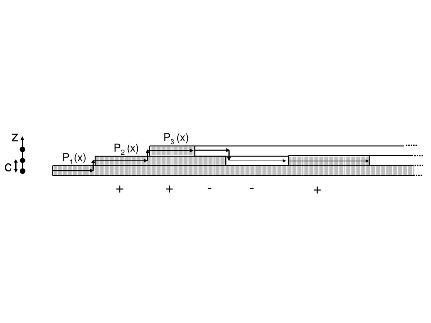
The above models (2 and N-level models) are limited to the analysis of a small roughness i.e. bounded to a few atomic layers. They are not suitable to describe the intensity scattered by a rough surface with a divergent height correlation function. An analytic method is proposed here (Fig 7) to calculate the scattered intensity assuming a random distribution of monoatomic upward and downward steps (height c) separated by terraces having a width distribution $P_{T}(x)$ Lapujoulade (1981); Pukite et al. (1985). Due to the divergence of the height correlation function, the whole scattered intensity is diffuse and no specular component has to be considered.

Similarly to the 2-level model, downward and upward steps are two complementary objects, which in this case do not alternate regularly but randomly with a probability $1/2$. The auto-correlation of the electronic density calculated for an upward step as starting object and for $x>0$ reads :

$$g_{+}(x,z) = \frac{1}{2}F_{+}(x,z)\otimes F_{+}(x,z)\otimes\Big{[}\delta(z)\times\delta(x)+\left(\frac{-\delta(z)+\delta(z-c)}{2}\right)\times P_{T}(x)+$$

$$+ \left(\frac{-\delta(z+c)+\delta(z)-\delta(z-c)+\delta(z-2c)}{4}\right)\times P_{T}(x)\otimes P_{T}(x)+...$$

$$...+ \frac{1}{2^{n+1}}\left(\sum_{k=0}^{n}\binom{n}{k}\Big{(}-\delta(z+(n-2k)c)+\delta(z+(n-1-2k)c)\Big{)}\right)\times P_{T}(x)^{\otimes n}+...\Big{]}$$

$$= \frac{1}{2}F(x,z)\otimes F(x,z)\otimes\Big{[}\delta(z)\times\delta(x)+$$

$$+ \sum_{n=0}^{\infty}\frac{\sum_{k=0}^{n}\binom{n}{k}\left(-\delta(z+(n-2k)c)+\delta(z+(n-1-2k)c)\right)}{2^{n+1}}\times P_{T}(x)^{\otimes n}\Big{]}$$

where $F_{+}(x,z)$ is the shape factor of an upward step, i.e. a semi-infinite row of atoms parallel to the terrace plane with positive electronic density. As for the two level model the downward steps is the opposite object, i.e. a semi-infinite row of atoms parallel to the terrace plane with negative electronic density $F_{-}(x,z)=-F_{+}(x,z)$. Therefore downward steps contribute in the above expression of the autocorrelation function of the electronic density as negative terms. The expression of the auto-correlation function is not very intuitive but the advantage of this approach is to get ride of the terrace width distribution. $\binom{n}{k}$ is a binomial coefficient which accounts for the all the possible combinations to reach a given height assuming random upward or downward steps.

The expression of the intensity is obtained by Fourier Transform of the auto-correlation function of the electronic density after adding the contribution of downward steps as starting object (replacing $\delta(z\pm nc)$ by $\delta(z\mp nc)$) in the above expression and then including the terms for $x<0$, i. e. the complex conjugate:

$$I(q_{x},q_{z}) = \mid\widetilde{F}(q_{x},q_{z})\mid^{2}\times$$ (18)

$$\times \left(1+\left[i\sin{(\frac{q_{z}c}{2})}e^{i\frac{q_{z}c}{2}}\widetilde{P}_{T}(q_{x})\sum_{n=0}^{\infty}\left[\widetilde{P}_{T}(q_{x})\cos{(q_{z}c)}\right]^{n}+c.c.\right]\right)$$

$$= \mid\widetilde{F}(q_{x},q_{z})\mid^{2}\left(1+\left[\frac{i\sin{(\frac{q_{z}c}{2})}e^{i\frac{q_{z}c}{2}}\widetilde{P}_{T}(q_{x})}{1-\widetilde{P}_{T}(q_{x})\cos{(q_{z}c)}}+c.c.\right]\right)$$

In a more compact way:

$$I(q_{x},q_{z})=\left[\frac{\mid\widetilde{F}_{cell}(q_{x},q_{z})\mid}{2\sin{(q_{x}a/2)}2\sin{(q_{z}c/2)}}\right]^{2}Re\left\{2\frac{(1-\cos{(q_{z}c)})(1-\widetilde{P}_{T}(q_{x}))}{1-\cos{(q_{z}c)}\widetilde{P}_{T}(q_{x})}\right\}$$ (19)

This result is in agreement with the generalized equation of the scattered intensity by a vicinal surface given in Eq. 9. The $\cos{(q_{z}c)}$ term in Eq. 19 is the characteristic function of the step heights distribution, which is simply in this case the sum of two delta functions in $-c$ and $+c$ weighted by $1/2$. Therefore Eq. 9, which is given for a vicinal surface, can, in fact, be applied for any step height distributions including negative height, i.e. downward steps. This equation but without the $\frac{1}{\sin(q_{z}c/2)^{2}}$ prefactor has been first obtained by Lu and Lagally (see Eq. $13$ of Ref Lu and Lagally (1982)) and then by Presicci and Lu in the special case of a geometric terrace width distribution (see Eq. $5$ of Ref Presicci and Lu (1984)). Note that the scattered intensity in anti-Bragg condition ($q_{z}c=\pi$) is the same for the randomly stepped surface and for the two-level model at half coverage as already mentioned by Henzler Henzler (1988). This ambiguity puts in evidence the necessity to measure the scattered intensity at different reciprocal space positions to fully characterize the surface roughness. For instance, in Fig 8, the $q_{x}$ position of the maxima corresponding to preferential terrace-terrace distances is a function of $q_{z}$. This result can be compared successfully to Fig. $5$ of Pimbley and Lu Pimbley and Lu (1985) calculated for a truncated geometric terrace size distribution. This can be understood through the interferences between the waves scattered by the terrace at different heights. This behavior does not occur for the two-level model for which the scattered intensity (off-specular) does not depend on $q_{z}$.

To characterize a rough surface, small angle scattering techniques are a common probe as they are preferentially sensitive to large length scales of the surface topography. In the small momentum transfer limit the intensity decreases as:

$$I(q_{x}\rightarrow 0,q_{z}\rightarrow 0)=\frac{\mid\widetilde{F}_{cell}(q_{x},q_{z})\mid^{2}}{(q_{x}D)^{2}+\frac{(q_{z}c)^{4}}{4}}$$ (20)

where D is the mean distance between nearest neighbor terraces. This result can be compared with a more general approach based on the use of the height correlation function Villain et al. (1985); Sinha et al. (1988); Robinson and Tweet (1992); Salanon and Lapujoulade (1994); Le Goff et al. (2003), $<(h(x)-h(0))^{2}>$, and in the special case of a 1D system.

$$I(q_{x},q_{z})=\left[\frac{\mid\widetilde{F}_{cell}(q_{x},q_{z})\mid}{2\sin{(q_{z}c/2)}}\right]^{2}\int_{-\infty}^{+\infty}e^{-(1-\cos(q_{z}c))<(h(x)-h(0))^{2}>}dx$$ (21)

To obtain an explicit expression the height correlation function has to be known. In the case of the paracrystal model, the asymptotic behavior of the height correlation function is a linear function of the distance if the first moments of the terrace width distribution exist (the distribution decays fast enough): $<(h(x)-h(0))^{2}>=x\frac{c^{2}}{D}$ where c and D are respectively the mean step height and the mean distance between adjacent steps. In this case the calculation of the intensity from Eq. 21 reads exactly as Eq. 20. Of course the main drawback of the paracrystal model is its one-dimensional character contrary to the calculation based on the height correlation function that holds naturally to two dimensions and is more appropriate for instance to describe roughening Villain et al. (1985); Le Goff et al. (2003). However for some cases as proposed in paragraph 3, the paracrystal approach can be used to describe 2D systems. The present calculation has also the advantage to evaluate the scattered intensity in the whole reciprocal space (not only in the small angle regime) and for any terrace width distributions.

II.5 The faceted surface

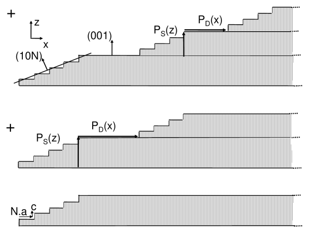
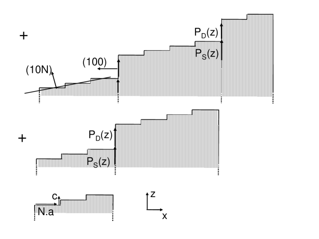
Surface instabilities towards faceting or step bunching have been widely studied for instance in the case of the electromigration-induced faceting of silicon vicinal surfaces Song et al. (1995) or under adsorption of foreign species Coati et al. (2005). A model is developed here to calculate the intensity scattered by a faceted surface exposing two types of facets with two sets of size distribution. As an example, one of the facet type is a dense crystallographic plane and the other one is a vicinal face. To make simple calculations, the angle between the terrace plane of the vicinal facet and the low index crystallographic plane of the other facet is either 0° (Fig 9) or 90°(Fig 10) and respectively referred to small-angle and large-angle faceting. Similar calculations can be performed for any other angle. The principle of the calculation is to consider an elementary object which is a vicinal facet semi-infinitely extended in the x-direction (resp. z-direction) for the small-angle (resp. large-angle) faceting. For a vicinal (10N) facet with S steps, in the small-angle faceting case, the form factor reads:

$$\widetilde{F}_{facet}(q_{x},q_{z}) = \widetilde{F}_{cell}(q_{x},q_{z})\left[\sum_{n=0}^{\infty}e^{inq_{x}a}\right]\left[\sum_{m=0}^{S-1}e^{im(q_{x}Na+q_{z}c)}\right]$$

$$= \widetilde{F}_{cell}(q_{x},q_{z})\left[\frac{e^{-iq_{x}a/2}}{-2i\sin(q_{x}a/2)}\right]\left[e^{-i\frac{(q_{x}Na+q_{z}c)(S-1)}{2}}\frac{\sin(\frac{(q_{x}Na+q_{z}c)S}{2})}{\sin(\frac{(q_{x}Na+q_{z}c)}{2})}\right]$$

And the interference function is (See Eq. 7):

$$S(q_{x},q_{z}) = Re\left\{\frac{1+e^{i(q_{x}Na+q_{z}c)S}\widetilde{P}_{D}(q_{x})}{1-e^{i(q_{x}Na+q_{z}c)S}\widetilde{P}_{D}(q_{x})}\right\}$$ (23)

Therefore the scattered intensity reads :

$$I(q_{x},q_{z}) = \left[\frac{\mid\widetilde{F}_{cell}(q_{x},q_{z})\mid}{(2\sin{(q_{x}a/2)}2\sin(\frac{(q_{x}Na+q_{z}c)}{2}))}\right]^{2}Re\left\{2\frac{(1-e^{i(q_{x}Na+q_{z}c)S})(1-\widetilde{P}_{D}(q_{x}))}{1-e^{i(q_{x}Na+q_{z}c)S}\widetilde{P}_{D}(q_{x})}\right\}$$

The previous result can be easily checked assuming that $S=1$ and $N=0$ which gives exactly the intensity scattered by the vicinal surface (Eq. 8). A more general expression of Eq. LABEL:facetedsmallangle1 can be obtained putting instead of $e^{i(q_{x}Na+q_{z}c)S}$, the characteristic function of the distribution of the number of steps, $\widetilde{P}_{S}$, per vicinal facet. It results in the following expression of the intensity :

$$I(q_{x},q_{z})=\left[\frac{\mid\widetilde{F}_{cell}(q_{x},q_{z})\mid}{(2\sin{(q_{x}a/2)}2\sin(\frac{(q_{x}Na+q_{z}c)}{2}))}\right]^{2}Re\left\{2\frac{(1-\widetilde{P}_{S}(q_{x}Na+q_{z}c))(1-\widetilde{P}_{D}(q_{x}))}{1-\widetilde{P}_{S}(q_{x}Na+q_{z}c)\widetilde{P}_{D}(q_{x})}\right\}$$ (25)

For the large-angle faceting a very similar expression is obtained :

$$I(q_{x},q_{z})=\left[\frac{\mid\widetilde{F}_{cell}(q_{x},q_{z})\mid 2\sin{(q_{x}Na/2)}}{(2\sin{(q_{x}a/2)}2\sin{(q_{z}c/2)}2\sin(\frac{(q_{x}Na+q_{z}c)}{2}))}\right]^{2}Re\left\{2\frac{(1-\widetilde{P}_{S}(q_{x}Na+q_{z}c))(1-\widetilde{P}_{D}(q_{z}))}{1-\widetilde{P}_{S}(q_{x}Na+q_{z}c)\widetilde{P}_{D}(q_{z})}\right\}$$ (26)

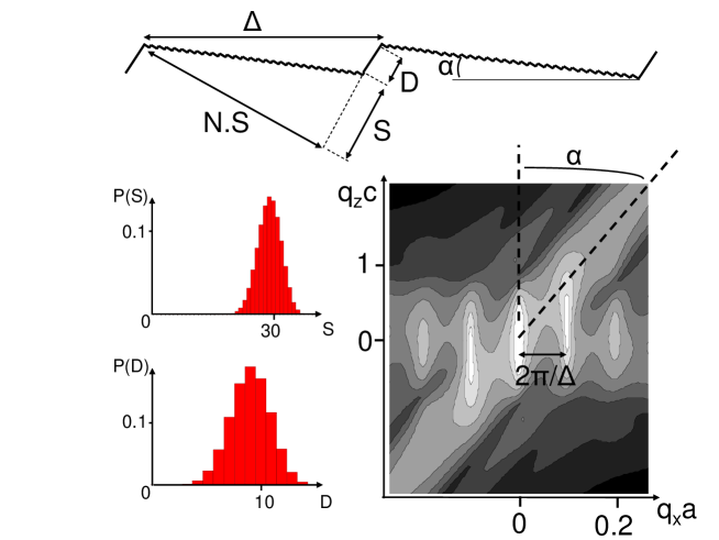
In Fig 11, a simulation of the scattered intensity close to a Bragg peak shows the main features of the diffuse scattering by a faceted surface. The regularity of the faceting gives rise to satellite peaks nearby the Bragg peak whereas at larger wavevector transfer, scattering rods perpendicular to facets are clearly visible.

III Towards two-dimensional analysis of scattering from surfaces

The simplicity of the previous calculations arises because of the one-dimensional character of the surface morphology. However, this is also its limitation since in general surface topography should be described in two dimensions. The appropriate generalization of this method to two dimensions is the Markov Random Field theory as pointed out by Lent and Cohen Lent and Cohen (1984). Without answering this question in the general case, a method is presented below to calculate the intensity scattered by 2D surfaces in few important cases : the kinked vicinal surface, the two-level vicinal surface and the step meandering on a vicinal surface.

III.1 The kinked vicinal surface

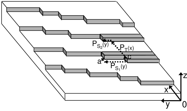
Analogously to the model of the vicinal surface the first step of the method is to find an elementary object that repeats regularly on the kinked vicinal surface. This object is a semi-infinite row parallel to the step (along the y-axis), starting at the kink (Fig 12). For instance, in the case of a monoatomic kink, the form factor of the elementary object is :

$$F_{\text{kinked vicinal}} = \widetilde{F}_{cell}(q_{x},q_{y},q_{z})\sum_{n=-\infty}^{0}e^{inq_{y}b+n\mu b}$$ (27)

$$= \frac{\widetilde{F}_{cell}(q_{x},q_{y},q_{z})e^{iq_{y}b/2}}{2i\sin(q_{y}b/2)}$$

In order to build the whole kinked vicinal surface, an infinite assembly of these objects are arranged along two main directions : the step edges (by definition) and perpendicularly to the steps to take into account any spatial correlations between kinks of neighboring steps. Both directions are decoupled by hypothesis and the kinks positions are given by the ideal 2D-paracrystal model Hosemann and Bagchi (1962); Eads and Millane (2001), assuming distance distributions between nearest neighbor kinks. However kinks (and steps) interact with each other via long range interactions (elastic, electrostatic) that yield a well defined separation between neighboring kinks. To solve this problem it would be necessary to take into account correlations with far neighbors which would make the calculation much more difficult. Our purpose is to give a simple and analytical calculation of the intensity scattered by a kinked vicinal surface assuming generic distributions of distances between nearest neighbors kinks. Of course a relevant choice of the distribution laws may allow partially taking into account the kink interaction.

In the direction parallel to the step edges the interference function is :

$$S_{\parallel}(q_{x},q_{y})=Re\left\{\frac{1+e^{iq_{x}a}\widetilde{P}_{{S_{1}}}(q_{y})}{1-e^{iq_{x}a}\widetilde{P}_{{S_{1}}}(q_{y})}\right\}$$ (28)

where $\widetilde{P}_{{S_{1}}}(q_{y})$ is the characteristic function of the distance separating two nearest neighbor kinks along the step edge and ${a}$ is the kink width (monoatomic in this case). This calculation is identical to the one for the vicinal surface model (see Eq. 7).

Similarly in the direction perpendicular to the steps, the interference function is given by:

$$S_{\perp}(q_{x},q_{y},q_{z})=Re\left\{\frac{1+e^{iq_{z}c}\widetilde{P}_{T}(q_{x})\widetilde{P}_{{S_{2}}}(q_{y})}{1-e^{iq_{z}c}\widetilde{P}_{T}(q_{x})\widetilde{P}_{{S_{2}}}(q_{y})}\right\}$$ (29)

where $\widetilde{P}_{T}(q_{x})$ and $\widetilde{P}_{{S_{2}}}(q_{y})$ are respectively the characteristic functions of the terrace widths distribution and kink positions along the upper (lower) step edges. $\widetilde{P}_{{S_{2}}}(q_{y})$ denotes the variations of the kink positions along adjacent step edges.

The expression of the intensity reads :

$$I(q_{x},q_{y},q_{z}) = \mid\widetilde{F}_{\textrm{kinked vicinal}}\mid^{2}\times S_{\parallel}(q_{x},q_{y})\times S_{\perp}(q_{x},q_{y},q_{z})$$ (30)

$$= \left[\frac{\mid\widetilde{F}_{cell}(q_{x},q_{y},q_{z})\mid}{2\sin(q_{y}b/2)}\right]^{2}\times$$

$$\times Re\left\{\frac{1+e^{iq_{x}a}\widetilde{P}_{S_{1}}(q_{y})}{1-e^{iq_{x}a}\widetilde{P}_{S_{1}}(q_{y})}\right\}\times$$

$$\times Re\left\{\frac{1+e^{iq_{z}c}\widetilde{P}_{T}(q_{x})\widetilde{P}_{S_{2}}(q_{y})}{1-e^{iq_{z}c}\widetilde{P}_{T}(q_{x})\widetilde{P}_{S_{2}}(q_{y})}\right\}$$

$$= \left[\frac{\mid\widetilde{F}_{cell}(q_{x},q_{y},q_{z})\mid}{2\sin(q_{x}a/2)2\sin(q_{y}b/2)2\sin(q_{z}c/2)}\right]^{2}\times$$

$$\times Re\left\{2\frac{(1-e^{iq_{x}a})(1-\widetilde{P}_{S_{1}}(q_{y}))}{1-e^{iq_{x}a}\widetilde{P}_{S_{1}}(q_{y})}\right\}\times$$

$$\times Re\left\{2\frac{(1-e^{iq_{z}c})(1-\widetilde{P}_{T}(q_{x})\widetilde{P}_{S_{2}}(q_{y}))}{1-e^{iq_{z}c}\widetilde{P}_{T}(q_{x})\widetilde{P}_{S_{2}}(q_{y})}\right\}$$

The first term in Eq. 30 consists of the multiplication of four terms : the form factor of the unit cell; the CTR, $1/2\sin{(q_{z}c/2)}$; the Terrace Truncation Rod, $1/2\sin{(q_{y}b/2)}$, which has already been highlighted in the case of the vicinal surface model and a new term, $1/2\sin{(q_{x}a/2)}$, which can be assigned to the truncation of an infinite step edge by a kink. Following previous terminology, it can be called Step Truncation Rod (STR). One should also notice that the scattered intensity is calculated in the whole reciprocal space (no specular scattering) as the whole sample volume (not only the surface) is taken into account in the calculation. As expected the intensity calculation shows two sets of scattering rods that are not perpendicular to each other and which correspond to the steps and kinks networks (Fig 13). Due to the miscut angle of the surface, the scattering rods shift along $q_{z}$, in the $q_{x}$ direction (steps) as well as in $q_{y}$ direction (kinks) in order to be perpendicular to the average surface plane. The $q_{y}$ shift is hardly visible as the orientation of the normal to the macroscopic surface plane depends slowly on the kinks density. For completeness about Eq.  30, a kink distribution can be considered (e.g. for non monoatomic kinks) replacing $e^{iq_{x}a}$ by the characteristic function of the kink width distribution. The same can be performed for the step height ($e^{iq_{z}c}$). In addition to the topographic characterization of a kinked vicinal surface, this model can be applied to calculate the scattered intensity during epitaxial growth at kink edges. The form factor of the elementary object has to be modified according to :

$$\widetilde{F}_{\text{kinked vicinal}} = \widetilde{F}_{cell}(q_{x},q_{y},q_{z})\sum_{n=-\infty}^{0}e^{inq_{y}b+n\mu b}+\widetilde{F}_{a}e^{i\vec{q}\vec{r}}$$ (31)

$$= \frac{\widetilde{F}_{cell}(q_{x},q_{y},q_{z})e^{iq_{y}b/2}}{2i\sin(q_{y}b/2)}+\widetilde{F}_{a}e^{i\vec{q}\vec{r}}$$

where $\widetilde{F}_{a}$ is the structure factor of the additional atom located at a vector $\vec{r}$ from the kink edges. Therefore intensity variations might be observed at anti-Bragg conditions, i.e. in the center of the reciprocal lattice nodes ($q_{x}a=q_{y}b=q_{z}c=\pi$). However this may be hardly measurable due to the very small number of atoms involved in the scattering process resulting from destructive interferences between the waves scattered by all the atoms. Indeed without foreign atoms the intensity results from only half of the atoms localized at the kinks positions. This is similar to X-ray scattering by a flat surface in anti-Bragg conditions where only half of the atoms of the last surface plane give a contribution (cubic case, Robinson and Tweet (1992)). In homoepitaxy, no intensity change is expected (the kinks cannot be rough). However in heteroepitaxy, the intensity can vary significantly depending on the structure factor of the foreign atom at its position with respect to the kink site.

III.2 The two-level vicinal surface

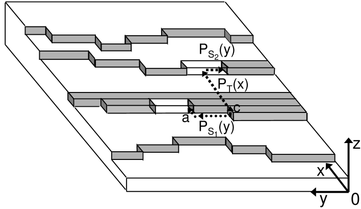
The aim of this part is to calculate the intensity scattered by a vicinal surface which has rough step edges Wollschläger and Larsson (1998); Tegenkamp et al. (2002). For that purpose we consider that the step edges can be described by a two-level model (Fig 14). Making use of previous results for the two-level model and for the vicinal surface the scattered intensity reads :

$$I(q_{x},q_{y}\neq 0,q_{z}) = \left[\frac{\mid\widetilde{F}_{cell}(q_{x},q_{y},q_{z})\mid}{2\sin(q_{y}b/2)}\right]^{2}\times$$ (32)

$$\times Re\left\{\frac{(1-\widetilde{P}_{+}(q_{y}))(1-\widetilde{P}_{-}(q_{y}))}{1-\widetilde{P}_{+}(q_{y})\widetilde{P}_{-}(q_{y})}\right\}\times$$

$$\times Re\left\{\frac{1+e^{iq_{z}c}\widetilde{P}_{T}(q_{x})\widetilde{P}_{S_{2}}(q_{y})}{1-e^{iq_{z}c}\widetilde{P}_{T}(q_{x})\widetilde{P}_{S_{2}}(q_{y})}\right\}$$

Where the first two terms at the right hand side of the equation has already been given in the case of the two-level model (see Eq. 12). Indeed a two-level model for step edges is equivalent to a one dimensional two-level model for a surface. The third term deals with the interference function for adjacent steps (see for instance Eq. 7 of the vicinal surface) with an additional term $\widetilde{P}_{S_{2}}(q_{y})$ which accounts for correlations between the positions of kinks at adjacent steps.

In this case the calculation of the scattered intensity is restricted to $q_{y}\neq 0$. Similarly to the two-level model one has to make an additional calculation for this case :

$$I(q_{x},0,q_{z})=\mid\widetilde{F}_{cell}(q_{x},0,q_{z})\mid^{2}\left|\frac{e^{-iq_{x}a/2}}{-2i\sin(q_{x}a/2)}+\theta e^{-iq_{x}a}\right|^{2}Re\left\{\frac{1+e^{iq_{z}c}\widetilde{P}_{T}(q_{x})}{1-e^{iq_{z}c}\widetilde{P}_{T}(q_{x})}\right\}$$ (33)

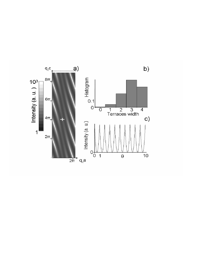
Where $\theta$ is the analogue of the coverage applied to a step edge. As already mentioned in the part dedicated to the one-dimensional analysis of vicinal surfaces, the roughness on step edges modifies the Terrace Truncation Rod in a way similar to the roughness on a flat surface for the CTR (Eq. 33). This remark calls for additional comments. For instance in the case of homoepitaxial growth on a vicinal surface, intensity oscillations may be observed in anti-Bragg conditions if the step edges are alternatively rough and smooth (Fig 15). To maximize the sensitivity to the roughness one has to be in anti-Bragg condition on the scattering rod of the step network ($q_{x}a=\pi$, $q_{y}b=0$, $q_{z}c=\pi$). Fig 15 reveals also that the scattering rods have a S shape. This can be assigned to the non integer value of the mean terrace size. Indeed, close to a Bragg peak, the scattering rods are perpendicular to the average surface plane. As the mean terrace size is not an integer, the scattering rods do not point towards a Bragg peak. Therefore there is a slight orientation change close to anti-Bragg conditions to connect two head-to-tail scattering rods Pimbley and Lu (1985). In addition shoulders in $q_{y}$ direction originating from a preferential distance between kinks are expected in the diffuse scattering (Eq. 32) as pointed out by Wollschläger et al. Wollschläger and Larsson (1998) and revealed experimentally by Tegenkamp et al. Tegenkamp et al. (2002) with SPA-LEED. This effect should be enhanced at half coverage of the step edges (maximum roughness) exactly in the same way as the two-level model for a surface (see Ref Croset and de Beauvais (1997)). In the case of heteroepitaxial growth at step edges on vicinal surfaces (e.g. Co/Pt(997) Gambardella et al. (2001)) complex interference effects are expected arising from the different scattering power between the substrate atoms and the adatoms. This model can be extended to the N-level vicinal surface. One has to add that the correlation between the morphologies of neighboring step edges may be adjusted thanks to the $\widetilde{P}_{{S_{2}}}(q_{y})$ function. It is related to the kink-kink relative displacement along two adjacent step edges. If the kinks positions are fully correlated, e.g. at identical $y$ position from step to step, $\widetilde{P}_{{S_{2}}}(q_{y})=1$. If the morphologies are independent $\widetilde{P}_{{S_{2}}}(q_{y})=\delta(q_{y})$. In this latter case, for $q_{y}\neq 0$ the scattered intensity is the incoherent sum of the contributions of independent step edges. For a detailed study of this case we refer to the work of Wollschläger et al. Wollschläger and Larsson (1998). Any intermediate case can be considered.

III.3 Step meandering on vicinal surfaces : the $\infty$-level vicinal surface model

The last example deals with step meandering on vicinal surfaces Villain et al. (1985). Instabilities on vicinal surfaces induced by specific growth conditions or an external stress may lead to step meandering Müller and Saùl (2004). Making use of previous results on randomly stepped surfaces and vicinal surfaces, the generalization to step meandering on vicinal surfaces is straightforward (Fig 16). The scattered intensity for a kink size $a$ and a step height $c$ is :

$$I(q_{x},q_{y},q_{z}) = \left[\frac{\mid\widetilde{F}_{cell}(q_{x},q_{y},q_{z})\mid}{2\sin(q_{x}a/2)2\sin(q_{y}b/2)}\right]^{2}\times$$ (34)

$$\times Re\left\{2\frac{(1-\cos{(q_{x}a)})(1-\widetilde{P}_{S_{1}}(q_{y}))}{1-\cos{(q_{x}a)}\widetilde{P}_{S_{1}}(q_{y})}\right\}\times$$

$$\times Re\left\{\frac{(1-e^{iq_{z}c})(1-\widetilde{P}_{T}(q_{x})\widetilde{P}_{S_{2}}(q_{y}))}{1-e^{iq_{z}c}\widetilde{P}_{T}(q_{x})\widetilde{P}_{S_{2}}(q_{y})}\right\}$$

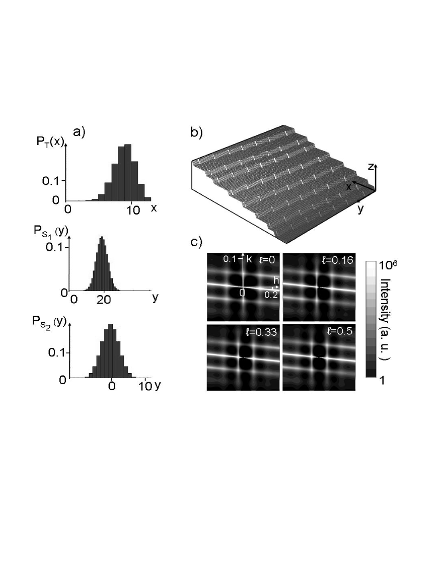
Where the first two terms on the right hand side of the equation are directly extracted from Eq. 19 of the randomly stepped surface. Indeed a step edge with random kinks is equivalent to the one dimensional randomly stepped surface model. The last term is the interference function of adjacent steps as seen previously for instance in the case of the kinked vicinal surface. A simulation of the intensity scattered by the step meandering model is shown in Fig 17. The intensity decreases much faster in the $q_{x}$ direction compared to the two-level vicinal surface model ($q_{x}^{-4}$ instead of $q_{x}^{-2}$) due to very rough step edges.

For this model one may wonder if steps may collide which is a non physical situation due to step-step repulsion. Even if the step distance distribution, i.e. $P_{T}(x)$, takes only positive values, steps may collide due to the $P_{S_{2}}(y)$ probability distribution for the kink-kink distance of adjacent steps. The effect of $P_{S_{2}}(y)$ is to decorrelate the kink positions of two neighbor steps. If one choose a very broad $P_{S_{2}}(y)$ probability distribution, a step may collide with an adjacent step. However this can be avoided by choosing a $P_{S_{2}}(y)$ probability distribution with a maximum $\mid y\mid$ displacement much smaller than the product of the kink-kink distance on a step edge times the number of kinks to fill the terrace width. This condition is not very restrictive but one can see that the limit case $P_{S_{2}}(y)=1$ does not fulfill this requirement. It leads to the diffraction by decorrelated steps as pointed out by Wollschläger et al. Wollschläger and Larsson (1998), but of course uncorrelated steps with random kinks on the step edges may collide. This remark on $P_{S_{2}}(y)$ applies also for the kinked vicinal surface model but not for the two-level vicinal surface model as the step-step fluctuations are confined in $\pm 1$ atomic distance and the non crossing condition for steps is easily fulfilled.

As for the kinked vicinal surface, the calculation provides the whole scattered intensity as their is no specular scattering. Of course the above expression can be generalized for any kink size and step height distributions. For instance it is straightforward to combine the randomly stepped model with a random distribution of kinks along the step edges just changing $e^{iq_{z}c}$ by $\cos{(q_{z}c)}$ in Eq. 34.

IV Lattice distortion

Until now no lattice distortion have been introduced and the crystallographic structure is the same at the surface and in the bulk. This assumption may be the most limiting one to quantitatively characterize surfaces with X-rays Prevot et al. (2003); Prévot and Croset (2004); Croset and Prevot (2006) as steps and kinks are intrinsic surface defects which stress the sample. To solve this problem, we suggest an approximate calculation of the scattered intensity which takes into account the strain field induced by steps and kinks assuming that the surface morphology is not perfectly periodic. To illustrate this point, let’s consider the case of a vicinal surface. For a perfectly periodic network of steps the strain field along only one atomic plane parallel to the terrace and starting at a step edge allows describing the strain field inside the whole sample volume Prévot and Croset . This aforementioned atomic plane is nothing else than the semi-infinite elementary object used to build the vicinal surface model (see Fig  2). Consequently the strain field calculation (e.g. in the framework of the linear elasticity theory) obtained for a perfect network of steps, may be applied to a slightly disordered one by simply using the form factor of the strained elementary object. Of course for highly disordered vicinal surfaces this calculation will not be appropriate. One has to be aware that a variation of the terrace size modifies not only the amplitude of the strain field but also the positions of the accidents of the displacement field which are located below the nearest neighbor steps. Therefore much caution is necessary to use this approximation. A similar result can be obtained for the kinked vicinal surface. The strain field induced by kinks on an ideal kinked vicinal surface (bi-periodic kinks network) can be obtained through the strain field calculation along only one atomic row parallel to a step edge and starting at a kink. Therefore an approximate calculation of the scattered intensity by a strained kinked vicinal surface can be obtained transferring this latter result to the elementary object. However contrary to the vicinal surface case, the strain field induced by an ideal kinked vicinal surface has not been calculated yet.

V Conclusion

We have developed a general simple method to calculate the intensity scattered by different kinds of surface morphologies that are not perfectly ordered. The model based on the paracrystal framework allows to recover previously published results on the scattering from vicinal surfaces, two-level models and randomly stepped surfaces. The most important result is the ability to characterize two dimensional surface structures from nearest neighbor distance distribution between steps or between kinks. The main hypothesis of the model consists in neglecting the long-range correlations between neighboring steps (or kinks) and, for the two dimensional models, in assuming that the step edge shape and the terrace width are independent. In the future, additional correlations should be considered, e.g. in the field of thin film growth between the size of neighboring terraces as highlighted first by M. C. Bartelt and J. W. Evans Bartelt et al. (1993). A step in this direction has been proposed in the case of the two-level model (see Ref Leroy et al. (2004)) which should be extended to more complicated surface morphologies.

Appendix A: Intensity scattered by a vicinal surface with a step height distribution

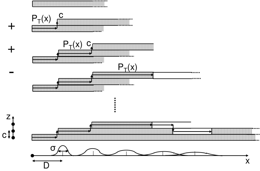
In this section, the intensity scattered by a vicinal surface with both step height $P_{H}$ and terrace width $P_{D}$ distributions is calculated (Fig  18).

The considered scattering object is a packing of H crystallographic planes, semi-infinite and parallel to the terrace. H is distributed according to the probability law $P_{H}$.

The auto-correlation function of the vicinal surface is (only the contribution of steps at $x>0$ is given):

$$g_{+}(x,z) = \iiiint_{-\infty}^{\infty}[F_{0}(x,z)\otimes F_{0}(x,z)\otimes\delta(z)\otimes\delta(x)+$$ (35)

$$+ F_{0}(x,z)\otimes F_{1}(x,z)\otimes\delta(z-\frac{H_{0}+H_{1}}{2})\otimes P_{D_{0}}(x)+$$

$$+ F_{0}(x,z)\otimes F_{2}(x,z)\otimes\delta(z-\frac{H_{0}+H_{2}}{2})\otimes P_{D_{0}}(x)\otimes[P_{H_{1}}(x)\otimes P_{D_{1}}(x)]+...$$

$$+ F_{0}(x,z)\otimes F_{n}(x,z)\otimes\delta(z-\frac{H_{0}+H_{n}}{2})\otimes P_{D_{0}}(x)\otimes[P_{H}(x)\otimes P_{D}(x)]^{\otimes^{n-1}}+...$$

$$+... ]\,\mathrm{d}P_{D_{0}}...\,\mathrm{d}P_{D_{n-1}}\,\mathrm{d}P_{H_{0}}...\,\mathrm{d}P_{H_{n}}...$$

where $F_{n}(x,z)$ is the shape of the $n^{th}$ object, i.e. $F_{n}(x,z)=1$ at the positions of the unit cells otherwise it is zero.

The intensity is obtained by Fourier transform of the auto-correlation function :

$$I(q_{x},q_{z})=FT\left\{g(x,z)\right\}$$ (36)

$$= \int_{H_{0}}\mid\widetilde{F}_{0}\mid^{2}+$$

$$+ \Big{[}\iiint_{H_{0},H_{1},D_{0}}\widetilde{F}_{0}(q_{x},q_{z})\widetilde{F}_{1}^{*}(q_{x},q_{z})e^{i(q_{z}\frac{(H_{0}+H_{1})c}{2})}e^{iq_{x}D_{0}a}+$$

$$+ \iiiint_{H_{0},H_{1},H_{2},D_{0},D_{1}}\widetilde{F}_{0}(q_{x},q_{z})\widetilde{F}_{2}^{*}(q_{x},q_{z})e^{i(q_{z}\frac{(H_{0}+H_{2})c}{2})}e^{iq_{z}D_{0}a}e^{i(q_{x}D_{1}a+q_{z}H_{1}c)}+...$$

$$...+ \iiiint_{H_{0},...,H_{n},D_{0},...,D_{n-1}}\widetilde{F}_{0}(q_{x},q_{z})\widetilde{F}_{n}^{*}(q_{x},q_{z})e^{i(q_{z}\frac{(H_{0}+H_{n})c}{2})}e^{iq_{z}D_{0}a}e^{i(q_{x}(D_{1}+...+D_{n-1})a+q_{z}(H_{1}+...+H_{n-1})c)}+...$$

$$...+ c.c.\Big{]}\,\mathrm{d}P_{D_{0}}...\,\mathrm{d}P_{D_{n-1}}\,\mathrm{d}P_{H_{0}}...\,\mathrm{d}P_{H_{n}}...$$

As the structure factor of the object is:

$$\widetilde{F}_{n}(q_{x},q_{z}) = \widetilde{F}_{cell}(q_{x},q_{z})\frac{e^{-iq_{x}a/2}}{-2i\sin{(q_{x}a/2)}}\frac{\sin{(q_{z}H_{n}c/2)}}{\sin{(q_{z}c/2)}}$$

$$= \widetilde{F}_{cell}(q_{x},q_{z})\frac{e^{-iq_{x}a/2}}{-2i\sin{(q_{x}a/2)}}\frac{e^{i(q_{z}H_{n}c/2)}-e^{-i(q_{z}H_{n}c/2)}}{2i\sin{(q_{z}c/2)}}$$

Therefore the scattered intensity reads:

$$I(q_{x},q_{z}) = \left[\frac{\mid\widetilde{F}_{cell}(q_{x},q_{z})\mid}{(2\sin{(q_{x}a/2)}2\sin{(q_{z}c/2)})}\right]^{2}\times$$

$$\times 2Re\left\{1-\widetilde{P}_{H}(q_{z}c)+\frac{(\widetilde{P}_{H}(q_{z}c)-1)(1-\widetilde{P}_{H}(q_{z}c))\widetilde{P}_{D}(q_{x}a)}{1-\widetilde{P}_{H}(q_{z}c)\widetilde{P}_{D}(q_{x}a)}\right\}$$

$$= \left[\frac{\mid\widetilde{F}_{cell}(q_{x},q_{z})\mid}{(2\sin{(q_{x}a/2)}2\sin{(q_{z}c/2)})}\right]^{2}Re\left\{2\frac{(1-\widetilde{P}_{H}(q_{z}c))(1-\widetilde{P}_{D}(q_{x}a))}{1-\widetilde{P}_{H}(q_{z}c)\widetilde{P}_{D}(q_{x}a)}\right\}$$

which is the expected result.

Appendix B: Discrete distributions and characteristic functions

Some examples of discrete distributions are given as well as their characteristic functions :

The Binomial distribution :

$$P_{p,N}(n) = \mathrm{C}_{N}^{n}p^{n}(1-p)^{N-n}$$

$$\widetilde{P}_{p,N}(q) = (1-p+pe^{iq})^{N}$$

The Poisson distribution :

$$P_{\nu}(n) = \frac{\nu^{n}}{n!}$$

$$\widetilde{P}_{\nu}(q) = e^{\nu(e^{iq}-1)}$$

The Geometric distribution :

$$P_{p}(n) = p(1-p)^{n}$$

$$\widetilde{P}_{p}(q) = \frac{p}{1-(1-p)e^{iq}}$$

For completeness, more complex distributions can be considered such as the hypergeometric distribution or the negative binomial distribution.

Figure 1: The vicinal surface described as a stacking of terraces. $P_{T}(x)$ is the terrace width distribution and $c$ is the step height.

Figure 2: The vicinal surface model. a) The elementary object is a semi-infinite plane starting at the step edge. b) and c), the vicinal surface is built step by step assuming a terrace width distribution $P_{T}(x)$. D is the average terrace width and $\sigma$ is the FWHM. The probability laws of having a distance separating the first, second and third neighbor steps are schematically drawn on the x axis. Due to an increase of disorder the probability laws broaden with the distance.

Figure 3: (a) Side view of a $(115)$ vicinal surface of a fcc crystal and scattered intensity (logarithmic scale) in the ($q_{x}0q_{z}$) plane for different terrace width distributions. From (b) to (d) the terrace width distribution gets larger and larger, making the scattering rods less and less narrow. $a$ is the lattice parameter, $a/2$ is the step height and $a/(2\sqrt{2})$ is the shift in $x$ of the lattice parameters of two adjacent terraces.

Figure 4: The two-level model is built step by step assuming alternating upward and downward steps. Terrace width distributions are respectively $P_{+}(x)$ and $P_{-}(x)$ for the high and the low levels. $D_{\pm}$ and $\sigma_{\pm}$ are respectively the average terrace width and the FWHM for both distributions. The probabilities of finding a distance $x$ separating a step up from a step down (or up) are schematically drawn on the x-axis.

Figure 5: a) Hard-Wall model (e.g. used for Helium Atom Scattering) for which only the last atomic layer is taken into account in the calculation of the scattered intensity. It results in an additional ($1-\cos(q_{z}c)$) term in the calculation of the scattered intensity. b) Model for X-ray scattering for which the whole sample volume has to be considered due to the very weak cross section. The difference in the off-specular scattering calculation consists in considering the atomic layer below the upper terraces.

Figure 6: The 3-level model is built assuming that from level 1 and level 3, the neighboring steps must be respectively upward and downward. From level 2, both upward and downward steps are equally probable. The terrace width distributions are $P_{1}(x)$, $P_{2}(x)$ and $P_{3}(x)$ for each level.

Figure 7: The rough surface can be seen as an infinite level model. The terrace width distribution is $P_{T}(x)$ $D$ is the mean distance and $\sigma$ is the FWHM, and c is the step height. Upward and downward steps are equally probable. As for the vicinal surface and the two-level model, the distributions of distances separating a $n^{th}$ neighbor step from an arbitrary step are schematically drawn on the x-axis. The FWHM of the distributions increases with the distance.

Figure 8: Reciprocal space map ($q_{x},q_{z}$) of a rough surface. D is the average distance between terraces. $\sigma/D=0.3$ (binomial distribution, see Appendix B)

Figure 9: Model of a faceted surface (small-angle faceting) showing two types of facets, a vicinal one of (10N) type and a low index one of (001) type. Two sets of size distributions are included: the number of steps $P_{S}$ of the vicinal facet and the number of unit cells $P_{D}$ of the low index facet.

Figure 10: Surface model for a large-angle faceting. Same as before but the low index facet is a (100) type.

Figure 11: Scattered intensity map ($q_{x},q_{z}$) in logarithmic scale (a decade of intensity separates each color change) of a faceted surface (large-angle faceting type). $q_{x}$ is parallel to the macroscopic surface plane and $q_{z}$ is perpendicular. The vicinal facet is of type (102). A schematic drawing of the surface morphology and the size distributions of $P(S)$ and $P(D)$ are given. $\Delta$ is the average periodicity of the faceting and $\alpha$ is the angle between the macroscopic surface plane and the most extended facet (vicinal facet).

Figure 12: The kinked vicinal surface model is built assuming that the elementary object is a semi-infinite row starting at the kink edge. Then the step edge is built from the kink-kink distance distribution, $P_{S_{1}}(y)$, and the terrace width is controlled by $P_{T}(x)$. $P_{S_{2}}(y)$ is an additional distribution to control the correlations of kinks positions of neighboring steps. a and c are respectively the kink size and the step height.

Figure 13: a) Step distance distribution $P_{T}(x)$, kink-kink distance distribution along the step edge $P_{S_{1}}(y)$, and kink-kink distance distribution along nearest neighbor steps $P_{S_{2}}(y)$. b) Simulation of the corresponding surface morphology. c) Intensity map scattered by this kinked vicinal surface at $q_{z}=0$.

Figure 14: The two-level vicinal surface model allows describing the step-edge of a vicinal surface as a two-level model. $P_{+}(y)$ and $P_{-}(y)$ are the width distributions of the higher and lower levels. As for the kinked vicinal surface model, the terrace width is controlled by $P_{T}(x)$ and the kink-kink distance along the y-direction for neighboring steps by $P_{S_{2}}(y)$.

Figure 15: a) Intensity map (logarithmic scale) of the two-level vicinal surface model in the $(q_{x}0q_{z})$ plane. b) Histogram of the terrace width used for the calculation. c) Intensity oscillations calculated in anti-Bragg condition (white cross on a). $\theta$ is the coverage rate of the step edge. One can notice the S shape of the scattering rods arising from the non integer value of the mean terrace size.

Figure 16: The step meandering model on a vicinal surface is built assuming that the step edge can be described by the infinite level model (kink-kink distance distribution: $P_{S_{1}}(y)$). The terrace width is controlled by $P_{T}(x)$ and the kink-kink distance along the neighboring step edge in the y-direction by $P_{S_{2}}(y)$.

Figure 17: a) Intensity map (logarithmic scale) of the step meandering vicinal surface model in the $(q_{x}0q_{z})$ plane. b) Histogram of the terrace width distribution. c) Histogram of the kink-kink distance distribution : $P_{S_{1}}(y)$. $P_{S_{2}}(y)$ is identical to $P_{S_{1}}(y)$ but centered around $y=0$. Compared to the two-level vicinal surface, the intensity decreases much faster in $q_{x}$ because the step edges are much more rough.

Figure 18: Vicinal surface model assuming a terrace width distribution ($P_{T}$) as well as a step height distribution ($P_{H}$). D and H are the mean terrace width and the mean step height and $\sigma_{T}$ and $\sigma_{H}$ are the FWHM of the probability laws. The FWHM of the probability to find two steps separated by a certain distance increases with this distance as schematically illustrated on the $x$-axis (same for the height, $z$-axis).

References

- Brune et al. (1998) H. Brune, M. Giovanni, K. Bromann, and K. Kern, Nature 394, 451 (1998).
- Leroy et al. (2005) F. Leroy, G. Renaud, A. Letoublon, R. Lazzari, C. Mottet, and J. Goniakowski, Phys. Rev. Lett. 95, 185501 (2005).
- Renaud et al. (2003) G. Renaud, R. Lazzari, C. Revenant-Brizard, A. Barbier, M. Noblet, O. Ulrich, F. leroy, J. Jupille, Y. Borenstzein, C. R. Henry, et al., Science 300, 1416 (2003).
- Braun et al. (2004) W. Braun, V. M. Kaganer, B. Jenichen, and K. H. Ploog, Phys. Rev. B (2004).
- Renaud et al. (1992) G. Renaud, P. H. Fuoss, J. Bevk, and B. S. Freer, Phys. Rev. B 45, 9192 (1992).
- Tegenkamp et al. (2002) J. Tegenkamp, J. Wollschläger, H. Pfnür, F.-J. Meyer zu Heringdorf, and M. Horn-von Hoegen, Phys. Rev. B 65, 235316 (2002).
- Sotto and Croset (2000) M. Sotto and B. Croset, Surf. Sci. 461, 78 (2000).
- (8) D. Farias and K.-H. Rieder, Rep. Prog. Phys. (????).
- Crottini et al. (1997) A. Crottini, D. Cvetko, L. Floreano, R. Gotter, A. Morgante, and F. Tommasini, Phys. Rev. Lett. 79, 1527 (1997).
- Ernst et al. (1992) H.-J. Ernst, F. Fabre, and J. Lapujoulade, Phys. Rev. B 46, 1929 (1992).
- Dulot et al. (2003) F. Dulot, B. Kierren, and D. Malterre, Thin Solid Films 428, 72 (2003).
- Robinson (1986) I. K. Robinson, Phys. Rev. B 33, 3830 (1986).
- Houston and Park (1971) J. E. Houston and R. L. Park, Surf. Sci. 29, 269 (1971).
- Lent and Cohen (1984) C. S. Lent and P. I. Cohen, Surf. Sci. 139, 121 (1984).
- Pukite et al. (1985) P. R. Pukite, C. S. Lent, and P. I. Cohen, Surf. Sci. 161, 39 (1985).
- Croset and de Beauvais (1997) B. Croset and C. de Beauvais, Surf. Sci. 384, 15 (1997).
- Uimin and Lindgård (1997) G. Uimin and P.-A. Lindgård, Acta Cryst. A 53, 15 (1997).
- Wollschläger (1997) J. Wollschläger, Surf. Sci. 383, 103 (1997).
- Hosemann and Bagchi (1962) R. Hosemann and S. N. Bagchi, Direct analysis of diffraction by matter (North-Holland Publishing Company, Amsterdam, 1962).
- Guinier and Fournet (1955) A. Guinier and G. Fournet, Small-angle scattering of X-rays (Jonh Wiley & Sons, New York, 1955).
- Welberry (1985) T. R. Welberry, Rep. Prog. Phys. 48, 1543 (1985).
- (22) S. Pflanz and W. Moritz, Acta Cryst. A (????).
- Croset and de Beauvais (1998) B. Croset and C. de Beauvais, Surf. Sci. 409, 403 (1998).
- Rao and Hibma (1991) G. H. Rao and T. Hibma, Surf. Sci. 250, 207 (1991).
- Vlieg et al. (1988) E. Vlieg, A. W. Denier van der Gon, J. F. Van der Veen, J. E. Macdonald, and C. Norris, Phys. Rev. Lett. 61, 2241 (1988).
- Hermans (1944) J. J. Hermans, Rec. Trav. Chim. 63, 211 (1944).
- Lapujoulade (1981) J. Lapujoulade, Surf. Sci. 108, 526 (1981).
- Lu and Lagally (1982) T. M. Lu and M. G. Lagally, Surf. Sci. 120, 47 (1982).
- Presicci and Lu (1984) M. Presicci and T. M. Lu, Surf. Sci. 141, 233 (1984).
- Henzler (1988) M. Henzler, The study of Epitaxy with Spot Profile Analysis of LEED (SPA-LEED) (Springer, 1988).
- Pimbley and Lu (1985) J. M. Pimbley and T. M. Lu, Surf. Sci. 159, 169 (1985).
- Villain et al. (1985) J. Villain, D. R. Grempel, and J. Lapujoulade, J. Phys. F: Met. Phys. 15, 809 (1985).
- Sinha et al. (1988) S. K. Sinha, E. B. Sirota, S. Garoff, and H. B. Stanley, Phys. Rev. B 38, 2297 (1988).
- Robinson and Tweet (1992) I. K. Robinson and D. J. Tweet, Rep. Prog. Phys. 55, 599 (1992).
- Salanon and Lapujoulade (1994) B. Salanon and J. Lapujoulade, Comput. Phys. Commun. 80, 32 (1994).
- Le Goff et al. (2003) E. Le Goff, L. Barbier, Y. Garreau, and M. Sauvage, Surf. Sci. 522, 143 (2003).
- Song et al. (1995) S. Song, S. G. J. Mochrie, and G. B. Stephenson, Phys. Rev. Lett. 74, 5240 (1995).
- Coati et al. (2005) A. Coati, J. Creuze, and Y. Garreau, Phys. Rev. B 72, 115424 (pages 10) (2005).
- Eads and Millane (2001) J. Eads and R. Millane, Acta. Cryst. A 57, 507 (2001).
- Wollschläger and Larsson (1998) J. Wollschläger and M. Larsson, Phys. Rev. B 57, 14937 (1998).
- Gambardella et al. (2001) P. Gambardella, A. Dallmeyer, K. Maiti, M. C. Malagoli, W. Eberhardt, K. Kern, and C. Carbone, Nature 416, 301 (2001).
- Müller and Saùl (2004) P. Müller and A. Saùl, Surf. Sci. Rep. 54, 157 (2004).
- Prevot et al. (2003) G. Prevot, P. Steadman, and S. Ferrer, Phys. Rev. B 67, 245409 (pages 6) (2003).
- Prévot and Croset (2004) G. Prévot and B. Croset, Phys. Rev. Lett. 92, 256104 (pages 4) (2004).
- Croset and Prevot (2006) B. Croset and G. Prevot, Phys. Rev. B 73, 045434 (pages 13) (2006).
- (46) G. Prévot and B. Croset, Submitted to Phys. Rev. B (????).
- Bartelt et al. (1993) N. C. Bartelt, T. L. Einstein, and E. D. Williams, Surf. Sci. 298, 421 (1993).
- Leroy et al. (2004) F. Leroy, R. Lazzari, and G. Renaud, Acta Cryst. A 60, 565 (2004).