The Pion-Photon Transition Distribution Amplitudes in the Nambu-Jona Lasinio Model

Abstract

We define the pion-photon Transition Distribution Amplitudes (TDA) in a field theoretic formalism from a covariant Bethe-Salpeter approach for the determination of the bound state. We apply our formalism to the Nambu - Jona Lasinio model, as a realistic theory of the pion. The obtained vector and axial TDAs satisfy all features required by general considerations. In particular, sum rules and polynomiality condition are explicitly verified. We have numerically proved that the odd coefficients in the polynomiality expansion of the vector TDA vanish in the chiral limit. The role of PCAC and the presence of a pion pole are explicitly shown.

I Introduction

Hard reactions provide important information for unveiling the structure of hadrons. The large virtuality, $Q^{2}$, involved in the processes allows the factorization of the hard (perturbative) and soft (non-perturbative) contributions in their amplitudes. Therefore these reactions are receiving great attention by the hadronic physics community. In the past, only total cross sections of inclusive processes or longitudinal asymmetries, that have simple parton model interpretations, were studied. The basic theoretical ingredients to be understood are diagonal Parton Distribution Functions (PDF) Jaffe:1996zw , governing the deep inclusive processes. In the recent years a new variety of processes, like the Deeply Virtual Compton Scattering, has been considered. These processes are governed by the Generalized Parton Distributions (GPD) Mueller:1998fv ; Radyushkin:1996nd ; Ji:1996ek ; Diehl:2003ny . From a theoretical point of view, PDFs are related to diagonal matrix elements of a bilocal operator from the initial hadron state to the same final hadron state (the same particle with the same momentum). The GPDs are related to the matrix elements of the same bilocal operator as in the previous case, where the initial and final hadron are the same particle, but have different momentum. The GPDs describe non-forward matrix elements of light-cone operators and therefore measure the response of the internal structure of the hadrons to the probes.

The generalization of parton distributions to the case where the initial and final states correspond to different particles has recently been proposed in Pire:2004ie ; Lansberg:2006fv . Such distributions are called Transition Distribution Amplitudes (TDA) since they have been introduced through hadron-photon transitions. In particular, the easiest case is to consider pion-photon TDA, governing processes like $\pi^{+}\pi^{-}\rightarrow\gamma^{\ast}\gamma$ or $\gamma^{\ast}\pi^{+}\rightarrow\gamma\pi^{+}$ in the kinematical regime where the virtual photon is highly virtual but with small momentum transfer.

The aim of this work is to calculate the pion-photon TDAs in a field theoretic scheme treating the pion as a bound state in a fully covariant manner using the Bethe-Salpeter equation. In this way we preserve all invariances of the problem. In order to perform a numerical study we will use the Nambu - Jona Lasinio (NJL) model to describe the pion structure. The NJL model is the most realistic model for the pion based on a local quantum field theory built with quarks. It respects the realizations of chiral symmetry and gives a good description of the low energy physics of the pion Klevansky:1992qe .

The NJL model is a non-renormalizable field theory and therefore a cut-off procedure has to be defined. We have chosen the Pauli-Villars regularization procedure because it respects all the symmetries of the problem. The NJL model together with its regularization procedure is regarded as an effective theory of QCD. Moreover, it has been used to tune coefficients of Chiral Perturbation Theory Bijnens:1995ww .

The NJL model has been used to describe the soft (non perturbative) part of the deep processes, while for the hard part conventional perturbative QCD must be used. It has been applied to the study of pion PDF Davidson:1994uv ; Davidson:2001cc ; Ruiz Arriola:2002bp and to the pion GPD Theussl:2002xp . In the chiral limit, its quark valence distribution is as simple as $q(x)=\theta\left(x\right)~{}\theta(1-x)$. Once evolution is taken into account, a good agreement is reached between the calculated PDF and the experimental one Davidson:1994uv . A more elaborated study of pion PDF is done in Ref. Noguera:2005cc using non local lagrangians Noguera:2005ej , which confirms that the result obtained in the NJL model for the PDF is a good approximation.

As GPDs, TDAs must satisfy sum rules. The vector and axial TDA are connected to the vector and axial form factors, $F_{V}$ and $F_{A},$ appearing in the $\pi^{+}\rightarrow\gamma e^{+}\nu$ process. In order to have a proper understanding of the axial TDA we will make the difference between two contributions to the axial current coming from the analysis of the amplitude for the pion radiative decay. The first one is originated from the internal structure of the hadron, in our case a pion. This contribution is the proper axial TDA. A second contribution is present and it can be understood as a manifestation of PCAC. The axial current can be coupled to a pion. This pion is a virtual one and its contribution will be present independently of the external hadron.

The polynomiality condition is also satisfied. We observe that, in the polynomial expansion of the moments of the vector TDA, the odd powers of $\xi$ are chirally suppressed and that they vanish in the chiral limit.

Previous studies of the axial and vector pion-photon TDA have been done using different quark models Tiburzi:2005nj ; Broniowski:2007fs . Both works parametrize the TDAs by means of Double Distributions.

This paper is organized as follows. In section II we establish the connection between the TDA and the vector and axial pion form factors, $F_{V}$ and $F_{A}$. In section III we define our approach for the TDA and we calculate them in the NJL model. In section IV we study the sum rules and the polynomiality condition of the TDAs. In section V we discuss our results and we finally give our conclusions in section VI.

II The pion-photon Transition Distribution Amplitudes

The pion-photon TDAs are connected, through sum rules, to the vector and axial-vector pion form factors, $F_{V}$ and $F_{A}$. Before giving a proper definition of the TDAs let us recall the definition of these form factors. They appear in the vector and axial vector hadronic currents contributing to the decay amplitude of the process $\pi^{+}\rightarrow\gamma e^{+}\nu$. The precise definitions of these currents are Moreno:1977kx ; Bryman:1982et :

$$\left\langle\gamma\left(p^{\prime}\right)\right|\bar{q}\left(0\right)\gamma_{\mu}\tau^{-}q\left(0\right)\left|\pi\left(p\right)\right\rangle=-i\,e\,\varepsilon^{\nu}\,\epsilon_{\mu\nu\rho\sigma}\,p^{\prime\rho}\,p^{\sigma}\,\frac{F_{V}\left(t\right)}{m_{\pi}}~{},$$ (1)

$$\left\langle\gamma\left(p^{\prime}\right)\right|\bar{q}\left(0\right)\gamma_{\mu}\gamma_{5}\tau^{-}q\left(0\right)\left|\pi\left(p\right)\right\rangle =e\,\varepsilon^{\nu}\left(p_{\mu}^{\prime}\,p_{\nu}-g_{\mu\nu}\,p^{\prime}.p\right)\frac{F_{A}\left(t\right)}{m_{\pi}}$$

$$+e\,\varepsilon^{\nu}\left(\left(p^{\prime}-p\right)_{\mu}\,p_{\nu}\frac{2\sqrt{2}f_{\pi}}{m_{\pi}^{2}-t}-\sqrt{2}f_{\pi}\,g_{\mu\nu}\right)~{},$$ (2)

with $f_{\pi}=93\operatorname{MeV},$ $\varepsilon^{0123}=1$ and $\tau^{-}=\left(\tau_{1}-i\,\tau_{2}\right)/2.$ All the structure of the decaying pion is included in the form factors $F_{V}$ and $F_{A}$. We observe that the vector current only contains a Lorentz structure associated with the $F_{V}$ form factor. The axial current is composed of two terms. The first one, defining $F_{A}$, gives the structure of the pion. The second one corresponds to the axial current for a point-like pion. It has two different contributions. The first one corresponds to a point-like coupling between the incoming pion, the outcoming photon and a virtual pion which is coupled to the axial current. It is depicted in the diagram of Fig. 1 and can be seen as a result of PCAC, because the axial current must be coupled to the pion. It isolates the pion pole contribution of the axial current in a model independent way. The second contribution of this term, proportional to $f_{\pi}\,g_{\mu\nu}$, corresponds to a pion-photon-axial current contact term. With these definitions, all the structure of the pion remains in the form factor $F_{A}$.

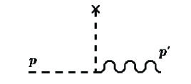
Figure 1: Pion pole contribution between the axial current (represented by a cross) and the photon-external pion vertex associated to the last contribution of equation (2).

Let us go now to TDAs. For their definition we introduce the light-cone coordinates $v^{\pm}=\left(v^{0}\pm v^{3}\right)/\sqrt{2}$ and the transverse components $\vec{v}^{\bot}=\left(v^{1},v^{2}\right)$ for any four-vector $v^{\mu}$. We define $P=\left(p+p^{\prime}\right)/2$ and the momentum transfer, $\Delta=p^{\prime}-p,$ therefore $P^{2}=m_{\pi}^{2}/2-t/4$ and $t=\Delta^{2}$. The skewness variable describes the loss of plus momentum of the incident pion, i.e. $\xi=\left(p-p^{\prime}\right)^{+}/2P^{+},$ and its value ranges between $t/\left(2m_{\pi}^{2}-t\right)<\xi<1$. Actually there is no symmetry relating the distributions for negative and positive $\xi$ which could have constrained the values of the skewness variable to be positive, like for GPDs. The vector and axial TDAs are the Fourier transform of the matrix element of the bilocal currents, $\bar{q}\left(-z/2\right)\gamma_{\mu}\left[\gamma_{5}\right]q\left(z/2\right)$, separated by a light-like distance. Then, they are directly related to the currents defined in Eqs. (1-2) through the sum rules:

$$\int_{-1}^{1}dx\int\frac{dz^{-}}{2\pi}e^{ixP^{+}z^{-}}\left.\left\langle\gamma\left(p^{\prime}\right)\right|\bar{q}\left(-\frac{z}{2}\right)\gamma_{\mu}\left[\gamma_{5}\right]\tau^{-}q\left(\frac{z}{2}\right)\left|\pi\left(p\right)\right\rangle\right|_{z^{+}=z^{\bot}=0}=\frac{1}{P^{+}}\left\langle\gamma\left(p^{\prime}\right)\right|\bar{q}\left(0\right)\gamma_{\mu}\left[\gamma_{5}\right]\tau^{-}q\left(0\right)\left|\pi\left(p\right)\right\rangle~{}.$$ (3)

With this connection we can introduce the leading twist decomposition of the bilocal currents. For that we introduce the light-front vectors $\bar{p}^{\mu}=P^{+}\left(1,0,0,1\right)/\sqrt{2}$ and $n^{\mu}=\left(1,0,0,-1\right)/\left(\sqrt{2}P^{+}\right).$ The explicit expressions for the pion and photon momenta in terms of their light-cone components are given by Eqs. (34) and (35). Then we have

$$\int\frac{dz^{-}}{2\pi}e^{ixP^{+}z^{-}}\left.\left\langle\gamma\left(p^{\prime}\right)\right|\bar{q}\left(-\frac{z}{2}\right)\hbox to0.0pt{$/$\hss}n\tau^{-}q\left(\frac{z}{2}\right)\left|\pi\left(p\right)\right\rangle\right|_{z^{+}=z^{\bot}=0}=\frac{i}{P^{+}}\,e\,\varepsilon^{\nu}\,\epsilon_{\mu\nu\rho\sigma}\,n^{\mu}\,P^{\rho}\,\Delta^{\sigma}\,\frac{V^{\pi^{+}}\left(x,\xi,t\right)}{\sqrt{2}f_{\pi}}~{},$$ (4)

$$\int\frac{dz^{-}}{2\pi}e^{ixP^{+}z^{-}}\left.\left\langle\gamma\left(p^{\prime}\right)\right|\bar{q}\left(-\frac{z}{2}\right)\hbox to0.0pt{$/$\hss}n\gamma_{5}\tau^{-}q\left(\frac{z}{2}\right)\left|\pi\left(p\right)\right\rangle\right|_{z^{+}=z^{\bot}=0} =\frac{1}{P^{+}}e\,\left(\vec{\varepsilon}^{\bot}\cdot\vec{\Delta}^{\bot}\right)\frac{A^{\pi^{+}}\left(x,\xi,t\right)}{\sqrt{2}f_{\pi}}$$

$$+\frac{1}{P^{+}}e\,\left(\varepsilon\cdot\Delta\right)\frac{2\sqrt{2}f_{\pi}}{m_{\pi}^{2}-t}~{}\epsilon\left(\xi\right)~{}\phi\left(\frac{x+\xi}{2\xi}\right)\quad,$$ (5)

where $\epsilon\left(\xi\right)$ is equal to $1$ for $\xi>0,$ and equal to $-1$ for $\xi<0$. Here $V\left(x,\xi,t\right)$ and $A\left(x,\xi,t\right)$ are respectively the vector and axial TDAs. They are defined as dimensionless quantities. From the condition (3) we observe that they obey the following sum rules:

$$\int_{-1}^{1}dx~{}V^{\pi^{+}}\left(x,\xi,t\right)=\frac{\sqrt{2}f_{\pi}}{m_{\pi}}F_{V}\left(t\right)~{},$$ (6)

$$\int_{-1}^{1}dx~{}A^{\pi^{+}}\left(x,\xi,t\right)=\frac{\sqrt{2}f_{\pi}}{m_{\pi}}F_{A}\left(t\right)~{},$$ (7)

which were firstly introduced in Refs. Pire:2004ie ; Lansberg:2006fv .

In the second term of Eq. (5), we have introduced the Pion Distribution Amplitude (PDA) $\phi\left(x\right).$ By definition the PDA is

$$\int\frac{dz^{-}}{2\pi}e^{i\left(x-\frac{1}{2}\right)p^{+}z^{-}}\left.\left\langle 0\right|\bar{q}\left(-\frac{z}{2}\right)\hbox to0.0pt{$/$\hss}n\gamma_{5}\tau^{-}q\left(\frac{z}{2}\right)\left|\pi\left(p\right)\right\rangle\right|_{z^{+}=z^{\bot}=0}=\frac{1}{p^{+}}i\sqrt{2}f_{\pi}\phi\left(x\right)\quad,$$ (8)

The PDA vanishes outside the region $x\in\left[0,1\right]$ and satisfies the normalization condition

$$\int_{0}^{1}dx~{}\phi\left(x\right)=1~{}.$$ (9)

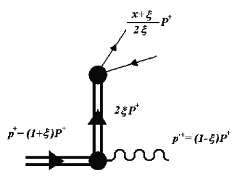
Figure 2: Pion pole contribution to the axial bilocal current corresponding to the last term of equation (5).

This second term has been introduced in order to isolate the pion pole contribution of the axial current in a model independent way, as we have done in Eq. (2) for the $\pi^{+}\rightarrow\gamma e^{+}\nu$ process. Therefore, all the structure of the pion remains in the TDA $A\left(x,\xi,t\right)$. It can be seen as a result of PCAC, because the axial current must be coupled to the pion. Therefore, this term is not a peculiarity of the pion-photon TDAs. A similar pion term will be present in the Lorentz decomposition in terms of distribution amplitudes of the axial current for any pair of external particles. A pion exchange contribution has already been analyzed in Mankiewicz:1998kg ; Penttinen:1999th for the axial helicity-flip GPD and, in Tiburzi:2005nj , a similar structure for the axial current has been obtained using different arguments. This term we have represented in Fig. 2 is only non-vanishing in the ERBL region, i.e. the $x\in\left[-\xi,\xi\right]$ region. The kinematics of this region allow the emission or absorption of a pion from the initial state, which is described through the PDA. And it can be seen from Fig. 2 that positive values of $\xi$ corresponds to an outcoming virtual pion, whereas negative values of $\xi$ describe an incoming virtual pion. The latter is related to the matrix element $\left\langle\pi\left(p\right)\right|\bar{q}\hbox to0.0pt{$/$\hss}n\gamma_{5}\tau^{-}q\left|0\right\rangle,$ instead of the one present in Eq. (8), what gives rise to the minus sign included in $\epsilon\left(\xi\right).$

III A field theoretic approach to the pion-photon TDA.

In Ref. Theussl:2002xp we have defined a method of calculation for the pion GPD in a field theoretical scheme, treating the pion as a bound state of quarks and antiquarks in a fully covariant manner using the Bethe-Salpeter equation. We apply here the same method for evaluating the pion-photon TDAs. This method has enormous advantages because it preserves all the physical invariances of the problem. Therefore, any property as sum rules or polynomiality is preserved.

As usual, we consider that the process is dominated by the hand-bag diagram. Each TDA has two related contributions, depending on which quark ($u$ or $d$) of the pion is scattered off by the deep virtual photon. In Fig. 3 we depicted the diagrams in which the photon scatters off the $u$-quark. We observe that there are two kinds of contributing diagrams. In the first one the $\bar{d}$-antiquark appears as the intermediate state, while in the second the bi-local current couples to a quark-antiquark pair coupled in the pion channel. The latter is present only for the axial current and includes the pion pole contribution.

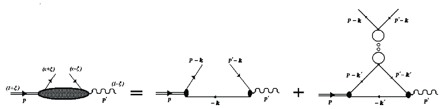
Figure 3: Diagrams contributing to the TDA. We have depicted diagrams in which a quark $u$ is change into a quark $d$ by the bilocal current. There are similar diagrams in which the antiquark $\bar{d}$ is changed into a $\bar{u}$

The details of the method of calculation are given in Ref. Theussl:2002xp . In the present case we obtain, from the first kind of diagram of Fig. 3, the following contributions

$$\int\frac{dz^{-}}{2\pi}e^{ixP^{+}z^{-}}\left.\left\langle\gamma\left(p^{\prime},\varepsilon\right)\left|\bar{q}\left(-\frac{z}{2}\right)\gamma^{\mu}\left[\gamma_{5}\right]\tau^{-}q\left(\frac{z}{2}\right)\right|\pi^{+}\left(p\right)\right\rangle\right|_{z^{+}=z^{\bot}=0}$$

$$=-e\int\frac{d^{4}k}{\left(2\pi\right)^{4}}\varepsilon_{\nu}\left\{-\delta\left(xP^{+}-\frac{1}{2}\left(p^{\prime+}+p^{+}-2k^{+}\right)\right)\right.$$

$$\mathbb{T}\mathrm{r}\left[\frac{1}{2}\left(\frac{1}{3}+\tau_{3}\right)\,\gamma^{\nu}\,iS\left(p^{\prime}-k\right)\,\gamma^{\mu}\left[\gamma_{5}\right]\tau^{-}\,iS\left(p-k\right)\,\phi^{\pi^{+}}\left(k,p\right)\,iS\left(-k\right)\right]$$

$$-\delta\left(xP^{+}-\frac{1}{2}\left(2k^{+}-p^{+}-p^{\prime+}\right)\right)$$

$$\left.\mathbb{T}\mathrm{r}\left[\frac{1}{2}\left(\frac{1}{3}+\tau_{3}\right)\,\gamma^{\nu}\,iS\left(k\right)\,\phi^{\pi^{+}}\left(k,p\right)\,iS\left(k-p\right)\,\gamma^{\mu}\left[\gamma_{5}\right]\tau^{-}\,iS\left(k-p^{\prime}\right)\right]\right\}\quad,$$ (10)

where $S\left(p\right)$ is the Feynman propagator of the quark and $\phi^{\pi^{+}}\left(k,p\right)$ is the Bethe-Salpeter amplitude for the pion. Here $\mathbb{T}\mathrm{r}()$ represents the trace over spinor, color and flavor indices. The first contribution in Eq. (10) is the one depicted in the first diagram of Fig. 3. The second contribution corresponds to a similar diagram but changing quarks $u$ and $d$. In the NJL model, $\phi^{\pi^{+}}\left(k,p\right)$ is as simple as

$$\phi^{\pi^{+}}\left(k,p\right)=-g_{\pi qq}\,\gamma_{5}\,\sqrt{2}\tau^{+}~{},$$ (11)

where $g_{\pi qq}$ is the pion-quark coupling constant defined in Eq.( 38).

The vector TDA has contribution only from this first kind of diagrams. We can express $V\left(x,\xi,t\right)$ as the sum of the active $u$-quark and the active $\bar{d}$-quark distributions. The first contribution will be proportional to the $d$’s charge, and the second contribution to the $u$’s charge. Therefore, we can write

$$V^{\pi^{+}}\left(x,\xi,t\right)=-\frac{1}{3}v_{u\rightarrow d}^{\pi^{+}}\left(x,\xi,t\right)+\frac{2}{3}v_{\bar{d}\rightarrow\bar{u}}^{\pi^{+}}\left(x,\xi,t\right)\quad.$$ (12)

Isospin relates these two contributions, $v_{\bar{d}\rightarrow\bar{u}}^{\pi^{+}}\left(x,\xi,t\right)=v_{u\rightarrow d}^{\pi^{+}}\left(-x,\xi,t\right).$ A direct calculation gives

$$v_{u\rightarrow d}^{\pi^{+}}\left(x,\xi,t\right)=8\,N_{c}\,f_{\pi}\,g_{\pi qq}\,m\,\tilde{I}_{3v}\left(x,\xi,t\right)\quad,$$ (13)

with

$$\tilde{I}_{3v}\left(x,\xi,t\right)=i\int\frac{d^{4}k}{\left(2\pi\right)^{4}}\,\delta\left(x-1+\frac{k^{+}}{P^{+}}\right)\frac{1}{\left(k^{2}-m^{2}+i\epsilon\right)\,\left[\left(p^{\prime}-k\right)^{2}-m^{2}+i\epsilon\right]\,\left[\left(p-k\right)^{2}-m^{2}+i\epsilon\right]}\quad.$$ (14)

In this integral, we first perform the integration over $k^{-}$. The pole structure of the integrand fixes two non-vanishing contributions to $v_{u\rightarrow d}^{\pi^{+}}\left(x,\xi,t\right)$, the first one in the region $\xi<x<1$, corresponding to the quark contribution, and the second in the region $-\xi<x<\xi,$ corresponding to a quark-antiquark contribution. Given the relation (12), the support of the entire vectorial TDA, $V^{\pi^{+}}\left(x,\xi,t\right)$, is therefore $x\in[-1,1]$. The analytical expression for (14) is given by Eq. (44). For the $\pi^{0}$, the contributions of the first type of diagram (Fig. 3) can be related to $v_{u\rightarrow d}^{\pi^{+}}\left(x,\xi,t\right)$

$$V_{u}^{\pi^{0}} =\frac{Q_{u}}{\sqrt{2}}\left(v_{u\rightarrow d}^{\pi^{+}}\left(x,\xi,t\right)+v_{u\rightarrow d}^{\pi^{+}}\left(-x,\xi,t\right)\right)\quad,$$

$$V_{d}^{\pi^{0}} =\frac{Q_{d}}{\sqrt{2}}\left(v_{u\rightarrow d}^{\pi^{+}}\left(x,\xi,t\right)+v_{u\rightarrow d}^{\pi^{+}}\left(-x,\xi,t\right)\right)\quad.$$ (15)

Turning our attention to the axial TDA, we find a new contribution arising from the second diagram of Fig. 3. This second contribution comes from the re-scattering of a $q\bar{q}$ pair in the pion channel. Therefore

$$\int\frac{dz^{-}}{2\pi}e^{ixP^{+}z^{-}}\left.\left\langle\gamma\left(p^{\prime},\varepsilon\right)\left|\bar{q}\left(-\frac{z}{2}\right)\gamma^{\mu}\gamma_{5}\tau^{-}q\left(\frac{z}{2}\right)\right|\pi^{+}\left(p\right)\right\rangle\right|_{z^{+}=z^{\bot}=0}$$

$$=(\text{\ref{3.01}})+\sum_{i}M^{i}\frac{2ig}{1-2g\Pi_{ps}\left(t\right)}N^{i}\quad,$$ (16)

where $i$ is an isospin index,

$$M^{i} =-e\int\frac{d^{4}k^{\prime}}{\left(2\pi\right)^{4}}\varepsilon_{\nu}\left\{-\mathbb{T}\mathrm{r}\left[\phi^{\pi^{+}}\left(k^{\prime},p\right)\,iS\left(-k^{\prime}\right)\frac{1}{2}\left(\frac{1}{3}+\tau_{3}\right)\,\gamma^{\nu}\,iS\left(p^{\prime}-k^{\prime}\right)\,i\gamma_{5}\tau^{i}\,iS\left(p-k^{\prime}\right)\,\right]\right.$$

$$\left.-\mathbb{T}\mathrm{r}\left[\,\phi^{\pi^{+}}\left(k^{\prime},p\right)\,iS\left(k^{\prime}-p\right)\,i\gamma_{5}\tau^{i}\,iS\left(k^{\prime}-p^{\prime}\right)\frac{1}{2}\left(\frac{1}{3}+\tau_{3}\right)\,\gamma^{\nu}\,iS\left(k^{\prime}\right)\right]\right\}~{},$$ (17)

$$N^{i}=-\int\frac{d^{4}k}{\left(2\pi\right)^{4}}\delta\left(xP^{+}-\frac{1}{2}\left(p^{\prime+}+p^{+}-2k^{+}\right)\right)\mathbb{T}\mathrm{r}\left[iS\left(p^{\prime}-k\right)\,\gamma^{\mu}\gamma_{5}\tau^{-}\,iS\left(p-k\right)\,i\gamma_{5}\tau^{i}\right]\quad,$$ (18)

and $\Pi_{ps}$ is the pseudoscalar polarization,

$$\Pi_{ps}\left(\Delta^{2}\right)=-i\int\frac{d^{4}k}{\left(2\pi\right)^{4}}\left\{\mathbb{T}\mathrm{r}\left[i\gamma_{5}\,iS\left(k\right)\,i\gamma_{5}\,iS\left(\Delta-k\right)\right]\right.\quad.$$ (19)

We can now evaluate the axial current in a straightforward way. Nevertheless, in order to extract the axial TDA we must subtract the pion pole contribution. We need for that the pion amplitude which, in the NJL model, is

$$\phi\left(x\right)=\frac{m\,g_{\pi qq}\,N_{c}}{4\pi^{2}\,f_{\pi}}\,\sum_{i=1}^{2}c_{i}\log\frac{\left[m^{2}-m_{\pi}^{2}x\left(1-x\right)\right]}{\left[m_{i}^{2}-m_{\pi}^{2}x\left(1-x\right)\right]}\quad~{}~{}~{}~{}~{}~{}0\leq x\leq 1~{}\quad,$$ (20)

where $c_{i}$ and $m_{i}$ are defined in the Appendix. Now, after a long but direct calculation, we obtain the expression for $A\left(x,\xi,t\right).$ As the vector TDA, $A\left(x,\xi,t\right)$ can be expressed as a sum of the contributions coming from the active $u$-quark and the active $\bar{d}$-quark. The first one will be proportional to the $d$’s charge and the second to the $u$’s charge.

$$A^{\pi^{+}}\left(x,\xi,t\right)=-\frac{1}{3}a_{u\rightarrow d}^{\pi^{+}}\left(x,\xi,t\right)+\frac{2}{3}a_{\bar{d}\rightarrow\bar{u}}^{\pi^{+}}\left(x,\xi,t\right)\quad.$$ (21)

Isospin relates these two contributions, $a_{\bar{d}\rightarrow\bar{u}}^{\pi^{+}}\left(x,\xi,t\right)=-a_{u\rightarrow d}^{\pi^{+}}\left(-x,\xi,t\right),$ where the minus sign is originated in the change in helicity produced by the $\gamma_{5}$ operator. The expression for $a_{u\rightarrow d}^{\pi^{+}}\left(x,\xi,t\right)$ depends on the sign of $\xi.$ In the $\left|\xi\right|<x<1$ region we have

$$a_{u\rightarrow d}^{\pi^{+}}\left(x,\xi,t\right) =-8\,N_{c}\,f_{\pi}\,g_{\pi qq}\,m\left\{\left(1+\frac{m_{\pi}^{2}\left(x-\xi\right)+\left(1-x\right)t}{2\xi m_{\pi}^{2}-t\left(1+\xi\right)}\frac{1+\xi}{1-\xi}\right)\tilde{I}_{3v}\left(x,\xi,t\right)\right.$$

$$+\frac{1}{2\xi m_{\pi}^{2}-t\left(1+\xi\right)}\left.\frac{1+\xi}{1-\xi}\frac{1}{16\pi^{2}}\sum_{i=1}^{2}c_{i}\left[\log\frac{m^{2}\left(m_{i}^{2}-\bar{z}\,m_{\pi}^{2}\right)}{m_{i}^{2}\left(m^{2}-\bar{z}\,m_{\pi}^{2}\right)}\right]\right\}\quad,$$ (22)

with the abbreviations $\bar{z}=\left(1-x\right)\left(\xi+x\right)/\left(1+\xi\right)^{2}$. And in the $-\left|\xi\right|<x<\left|\xi\right|$ region we have

$$a_{u\rightarrow d}^{\pi^{+}}\left(x,\xi,t\right) =-8\,N_{c}\,f_{\pi}\,g_{\pi qq}\,m\left\{\left(1+\frac{m_{\pi}^{2}\left(x-\xi\right)+\left(1-x\right)t}{2\xi m_{\pi}^{2}-t\left(1+\xi\right)}\frac{1+\xi}{1-\xi}\right)\tilde{I}_{3v}\left(x,\xi,t\right)\right.$$

$$+\frac{\epsilon\left(\xi\right)}{1-\xi}\frac{1}{16\pi^{2}}\sum_{i=1}^{2}c_{i}\left[\frac{1+\xi}{2\xi m_{\pi}^{2}-t\left(1+\xi\right)}\log\frac{\left(4\xi^{2}m^{2}-\bar{x}\,t\right)\left(m_{i}^{2}-\bar{y}\,m_{\pi}^{2}\right)}{\left(4\xi^{2}m_{i}^{2}-\bar{x}\,t\right)\left(m^{2}-\bar{y}\,m_{\pi}^{2}\right)}\right.$$

$$+\left.\frac{2}{t-m_{\pi}^{2}}\left.\log\frac{\left(4\xi^{2}m^{2}-\bar{x}\,t\right)\left(4\xi^{2}m_{i}^{2}-\bar{x}\,m_{\pi}^{2}\right)}{\left(4\xi^{2}m_{i}^{2}-\bar{x}\,t\right)\left(4\xi^{2}m^{2}-\bar{x}\,m_{\pi}^{2}\right)}\right]\right\}\quad,$$ (23)

where $\bar{x}=\left(\xi^{2}-x^{2}\right)$ and $\bar{y}=\bar{z}$ for $\xi>0$ and $\bar{y}=0$ for $\xi<0$.

The expressions for both the vector and axial TDAs in the chiral limit, i.e. $m_{\pi}=0$, are well defined. In particular, for $t=0$, we find the following simple expression for $v_{u\rightarrow d}^{\pi^{+}}(x,\xi,t)$

$$v_{u\rightarrow d}^{\pi^{+}}(x,\xi,0)=\sqrt{2}\,f_{\pi}\,6\,F_{V}^{\pi^{+}\chi}(0)\,\left[\theta(\xi^{2}-x^{2})\,\,\frac{x+\left|\xi\right|}{2\left|\xi\right|(1+\left|\xi\right|)}\,+\,\theta(x-\left|\xi\right|)\theta(1-x)\frac{1-x}{1-\xi^{2}}\right]\quad,$$ (24)

where $F_{V}^{\pi^{+}\chi}(0)$ is the chiral limit of the vector pion form factor at zero momentum transfer $F_{V}^{\pi^{+}\chi}(0)=\lim_{m_{\pi}\rightarrow 0}F_{V}^{\pi^{+}}(0)/m_{\pi}=0.17\operatorname{GeV}^{-1}$.

A similar expression is obtained for $a_{u\rightarrow d}^{\pi^{+}}(x,\xi,t)$ in the chiral limit for $t=0$

$$a_{u\rightarrow d}^{\pi^{+}}(x,\xi,0) =-\sqrt{2}\,f_{\pi}\,6\,F_{A}^{\pi^{+}\chi}(0)\,\left[\theta(\xi^{2}-x^{2})\,\epsilon\left(\xi\right)\,\frac{\left(\xi-x\right)}{4\xi^{2}(1+\left|\xi\right|)}\left(x+\xi+\left(x-\xi\right)\frac{\left|\xi\right|-\xi}{(1+\left|\xi\right|)}\right)\right.\,\,$$

$$+\,\left.\theta(x-\left|\xi\right|)\theta(1-x)\frac{(1-x)(x-\xi)}{(1-\xi^{2})(1-\xi)}\right]\quad,$$ (25)

with $F_{A}^{\pi^{+}\chi}(0)$ the axial form factor at $t=0$ in the chiral limit $F_{A}^{\pi^{+}\chi}(0)=\lim_{m_{\pi}\rightarrow 0}F_{A}^{\pi^{+}}(0)/m_{\pi}=F_{V}^{\pi^{+}\chi}(0)$.

IV Sum rules and polynomiality

The vector TDA of the $\pi^{+}$ must obey the sum rule given in Eq. (6) with the expression of the vector pion form factor in the NJL model given by Eq. (40). We have numerically recovered the sum rule for different $t$ values. In particular we obtain the value $F_{V}^{\pi^{+}}(0)=0.0242$ for the vector form factor at $t=0$, which is in agreement with the experimental value $F_{V}(0)=0.017\pm 0.008$ given in Yao:2006px .

The $\pi^{0}$ distribution must satisfy the following sum rule Pire:2004ie

$$\int_{-1}^{1}dx\,\left(Q_{u}\,V_{u}^{\pi^{0}}(x,\xi,t)-Q_{d}\,V_{d}^{\pi^{0}}(x,\xi,t)\right)=\sqrt{2}\,f_{\pi}\,F_{\pi\gamma^{\ast}\gamma}(t)\qquad.$$ (26)

A theoretical prediction of the $\pi^{0}$ form factor value is given in Brodsky:1981rp . In particular, at $t=0$, the value $F_{\pi\gamma^{\ast}\gamma}(0)=0.272$ GeV^-1 is found. The neutral pion form factor is directly related to the $\pi^{+}$ vector form factor so that the sum rule is satisfied. We obtain the value $F_{\pi\gamma^{\ast}\gamma}(0)=0.244~{}$GeV^-1. In Gronberg:1997fj , a dipole parametrization based on experimental data is proposed for the $t$-dependence of $F_{\pi\gamma^{\ast}\gamma}\left(t\right)$, obtaining for the dipole mass $\Lambda=0.77$ GeV. We have found that, for small values of $t,$ the NJL neutral pion form factor can be parametrized in a dipole form with $\Lambda=0.81$ GeV.

The axial TDA obeys the sum rules given by Eq. (7) with the axial form factor given in the NJL model by Eq. (42). This sum rule is satisfied for different $t$ values. The numerical results also coincide. In particular we obtain $F_{A}^{\pi^{+}}(0)=0.0239$ for the axial form factor at $t=0$, which is about twice the value $F_{A}^{\pi^{+}}(0)=0.0115\pm 0.0005$ given by the PDG Yao:2006px .

We expect TDAs to obey the polynomiality condition. However no time reversal invariance enforces the polynomials to be even in the $\Delta$-momenta like for GPDs. That means that the polynomials should be “complete”, i.e. they should include all powers in $\xi$,

$$\int_{-1}^{1}dx\,x^{n-1}\,V(x,\xi,t)=\sum_{i=0}^{n-1}\,C_{n,i}(t)\,\xi^{i}\quad.$$ (27)

$n$	1	2	3	4
	$C_{1,0}\left(t\right)$	$\begin{array}[c]{rr}C_{2,0}\left(t\right)&C_{2,1}\left(t\right)\end{array}$	$\begin{array}[c]{rrr}C_{3,0}\left(t\right)&C_{3,1}\left(t\right)&C_{3,2}\left(t\right)\end{array}$	$\begin{array}[c]{rrrr}C_{4,0}\left(t\right)&C_{4,1}\left(t\right)&C_{4,2}\left(t\right)&C_{4,3}\left(t\right)\end{array}$
$\begin{array}[c]{c}m_{\pi}=0\end{array}$
$\begin{array}[c]{l}t=0\\ t=-0.5\\ t=-1.0\end{array}$	$\begin{array}[c]{l}22.6\\ 13.7\\ \lx@intercol\hfil 10.4\lx@intercol\end{array}$	$\begin{array}[c]{ll}-22.6&\hskip 2.84544pt0.0\\ -16.3&\hskip 2.84544pt0.0\\ \lx@intercol\hfil-13.4\lx@intercol&\lx@intercol\hfil 0.0\lx@intercol\end{array}$	$\begin{array}[c]{lll}3.77&\hskip 8.5359pt0.0&\hskip 8.5359pt3.77\\ \lx@intercol\hfil 3.00\lx@intercol&\hskip 8.5359pt0.0&\lx@intercol\hfil 2.43\lx@intercol\\ \lx@intercol\hfil 2.57\lx@intercol&\lx@intercol\hfil 0.0\lx@intercol&\lx@intercol\hfil 1.90\lx@intercol\end{array}$	$\begin{array}[c]{llll}-6.7&\hskip 8.5359pt0.0&\hskip 8.5359pt-6.7&\hskip 8.5359pt0.0\\ -5.7&\hskip 8.5359pt0.0&\hskip 8.5359pt-4.9&\hskip 8.5359pt0.0\\ -5.0&\lx@intercol\hfil 0.0\lx@intercol&\lx@intercol\hfil-4.0\lx@intercol&\lx@intercol\hfil 0.0\lx@intercol\end{array}$
$\begin{array}[c]{c}m_{\pi}=140\end{array}$
$\begin{array}[c]{l}t=0\\ t=-0.5\\ t=-1.0\end{array}$	$\begin{array}[c]{l}22.7\\ \lx@intercol\hfil 13.7\lx@intercol\\ \lx@intercol\hfil 10.3\lx@intercol\end{array}$	$\begin{array}[c]{ll}-22.9&\hskip 8.5359pt0.44\\ \lx@intercol\hfil-16.4\lx@intercol&\lx@intercol\hfil 0.25\lx@intercol\\ \lx@intercol\hfil-13.4\lx@intercol&\lx@intercol\hfil 0.19\lx@intercol\end{array}$	$\begin{array}[c]{lll}3.80&\hskip 8.5359pt-0.10&\hskip 8.5359pt3.67\\ \lx@intercol\hfil 3.00\lx@intercol&\lx@intercol\hfil-0.06\lx@intercol&\lx@intercol\hfil 2.43\lx@intercol\\ \lx@intercol\hfil 2.57\lx@intercol&\lx@intercol\hfil-0.05\lx@intercol&\lx@intercol\hfil 1.87\lx@intercol\end{array}$	$\begin{array}[c]{llll}-6.8&\hskip 5.69046pt0.19&\hskip 8.5359pt-6.8&\hskip 5.69046pt0.12\\ -5.7&\hskip 5.69046pt0.13&\hskip 8.5359pt-4.9&\hskip 5.69046pt0.08\\ -5.0&\hskip 5.69046pt0.11&\hskip 8.5359pt-4.0&\lx@intercol\hfil 0.06\lx@intercol\end{array}$

Table 1: Coefficients of the polynomial expansion for the vector TDA. The pion mass is expressed in MeV and $t$ is expressed in GeV². Notice that the coefficients have to be multiplied by $10^{-3}$.

However, in the chiral limit and for $t=0$, we have analytically found that the odd powers in $\xi$ go to zero for the polynomial expansion of the vector TDA. A study of the polynomiality in the limit given in Eq. (24) leads to the following analytical expression for the coefficients $C_{n,2i}^{\chi}(t)$

$$C_{n,2i}^{\chi}(0)=\sqrt{2}\,f_{\pi}\,\,2\,F_{V}^{\pi^{+}\chi}(0)\,\left(-1+2(-1)^{n-1}\right)\,\left(\frac{1}{n}-\frac{1}{n+1}\right)\quad.$$ (28)

Notice they do not depend on $i$. We have numerically tested the polynomiality and obtained it. We observe that the coefficients for the odd powers in $\xi$ are of one order of magnitude smaller than those for the even powers in $\xi$. In particular we have numerically proved that, in the chiral limit, the polynomials only contain even powers in $\xi$ for any value of $t,$

$$\int_{-1}^{1}dx\,x^{n-1}\,[\lim_{m_{\pi}\rightarrow 0}V(x,\xi,t)]=\sum_{i=0}^{[\frac{n-1}{2}]}\,C_{n,2i}^{\chi}(t)\,\xi^{2i}\quad.$$ (29)

The coefficients in the chiral limit, Eq. (29), as well as the coefficients for $m_{\pi}=140$ MeV, Eq. (27), we numerically obtained are given in Table 1.

The $\xi$-dependence of the moments of the axial TDA $A(x,\xi,t)$ also has a polynomial form. Those polynomials contain all the powers in $\xi$, i.e. even and odd,

$$\int_{-1}^{1}dx\,x^{n-1}\,A(x,\xi,t)=\sum_{i=0}^{n-1}\,C_{n,i}^{\prime}(t)\,\xi^{i}\quad.$$ (30)

An analytic study of the polynomiality in the limit given in Eq. (25) confirms that all the powers in $\xi$ have to be present. The analytic values for the coefficients in this specific limit are

$$C_{n,2i}^{\prime\chi}(0) =\sqrt{2}\,f_{\pi}\,\,2\,F_{A}^{\pi^{+}\chi}(0)\,\left(1+2(-1)^{n-1}\right)\,\frac{n-2i}{n(n+1)(n+2)}\quad,$$

$$C_{n,2i+1}^{\prime\chi}(0) =\sqrt{2}\,f_{\pi}\,\,2\,F_{A}^{\pi^{+}\chi}(0)\,\left(1+2(-1)^{n-1}\right)\,\frac{-2(i+1)}{n(n+1)(n+2)}\quad,$$ (31)

which is in agreement with those numerically obtained. The coefficients of the polynomial expansions in the chiral limit are very close to those obtained for the physical values of the pion mass. In Table 2, the coefficients $C_{n,i}^{\prime}(t)$ are therefore shown only for $m_{\pi}=140\operatorname{MeV}$. The polynomiality property of the term containing the pion DA can also be studied. The $t$-dependence only comes from the pion pole. We can therefore write a general relation about the polynomiality property of the whole axial bilocal matrix element

$$\int_{-1}^{1}dx\,x^{n-1}\,\int\frac{dz^{-}}{2\pi}\,e^{ixp^{+}z^{-}}\,\langle\gamma(P^{\prime})|\bar{q}\left(-\frac{z}{2}\right)\,\gamma_{\mu}n^{\mu}\gamma_{5}\,\tau^{-}q\left(\frac{z}{2}\right)|\pi(P)\rangle\,\,|_{z^{+}=z^{\perp}=0}=\frac{1}{p^{+}}\,e\,(\varepsilon.\Delta)\,\frac{1}{\sqrt{2}f_{\pi}}\,\sum_{i=0}^{n}\,C_{n,i}^{{}^{\prime\prime}}(t)\,\xi^{i}\quad.$$ (32)

$n$	1	2	3
	$C^{\prime}_{1,0}\left(t\right)$	$\begin{array}[c]{rr}C^{\prime}_{2,0}\left(t\right)&C^{\prime}_{2,1}\left(t\right)\end{array}$	$\begin{array}[c]{rrr}C^{\prime}_{3,0}\left(t\right)&C^{\prime}_{3,1}\left(t\right)&C^{\prime}_{3,2}\left(t\right)\end{array}$
$\begin{array}[c]{c}m_{\pi}=140\end{array}$
$\begin{array}[c]{l}t=0\\ t=-0.5\\ t=-1.0\end{array}$	$\begin{array}[c]{l}22.4\\ \lx@intercol\hfil 16.1\lx@intercol\\ \lx@intercol\hfil 13.2\lx@intercol\end{array}$	$\begin{array}[c]{ll}-3.77&\hskip 5.69046pt4.00\\ \lx@intercol\hfil-2.97\lx@intercol&\lx@intercol\hfil 2.57\lx@intercol\\ \lx@intercol\hfil-2.53\lx@intercol&\lx@intercol\hfil 1.97\lx@intercol\end{array}$	$\begin{array}[c]{lll}6.8&\hskip 5.69046pt-4.9&\hskip 5.69046pt2.3\\ \lx@intercol\hfil 5.7\lx@intercol&\lx@intercol\hfil-3.5\lx@intercol&\lx@intercol\hfil 1.7\lx@intercol\\ \lx@intercol\hfil 5.0\lx@intercol&\lx@intercol\hfil-2.8\lx@intercol&\lx@intercol\hfil 1.3\lx@intercol\end{array}$

Table 2: Coefficients of the polynomial expansion for the axial TDA. The pion mass is expressed in MeV and $t$ is expressed in GeV². Notice that the coefficients have to be multiplied by $10^{-3}$.

V Discussion.

In Figs. 4 and 5, the vector and axial TDAs are plotted in function of $x$ for several values of $\xi$ and $t$. In these figures, the $u$-quark contributes to the TDAs in the region of $x$ going from $-\left|\xi\right|$ to $1$ and the $d$-antiquark going from $-1$ to $\left|\xi\right|.$ Therefore, for $x\in\left[\left|\xi\right|,1\right]$ ($x\in\left[-1,-\left|\xi\right|\right]$) only $u$-valence quarks ($d$-valence antiquarks) are present (DGLAP regions). Besides, TDAs in the $-\left|\xi\right|<x<\left|\xi\right|$ region (ERBL region) receive contributions from both type of quarks. For the vector TDA, we observe in figure 4 that the position of the maxima is given by the $\xi$ value, separating explicitly the ERBL region from the DGLAP regions. The vector TDA is positive (negative) for negative (positive) values of $x$ with the change of sign occurring around $x=0$. This change in the sign of the vector TDA is originated in the presence of the electric charge of the quarks in Eq.(12).

The process involved in the calculation of the TDAs allows negative values of the skewness variable. In the chiral limit, the skewness variable goes from $\xi=-1$ to $\xi=1,$ for any value of $t$. In the chiral limit, the vector TDA for a negative value of $\xi$ is equal to the vector TDA for $\left|\xi\right|$. This can be seen from the polynomiality expansion in this limit, Eq. (29), which has only even powers of $\xi.$ For the physical value of the pion mass, negative values of $\xi$ are bounded by $t/\left(2m_{\pi}^{2}-t\right)<\xi.$ For each allowed value of $\xi$, we found that the numerical value of $V\left(x,-\left|\xi\right|,t\right)$ is close to $V\left(x,\left|\xi\right|,t\right),$ due to the smallness of the coefficients of the odd powers of $\xi$ in the polynomial expansion (27).

Analyzing the axial TDAs, plotted in Fig. 5, we observe two different behaviours depending on the sign of $\xi$. For positive $\xi,$ the position of the minima is given by the value of the skewness variable while the position of the maxima is always $x\simeq 0$ in the ERBL region and $x\simeq\pm(1+\xi)/2$ in the DGLAP regions. For negative $\xi,$ the value of the axial TDA at $x=\pm\xi$ is important and in some cases is a maximum and, in the ERBL region, $A\left(x,\xi,t\right)$ presents a minimum near $x=0.$ As we have previously shown, the axial TDA in the ERBL region receives contributions from two different diagrams, depicted in Fig. 3. In the second of these diagrams, a virtual quark-antiquark interacting pair in the pion channel appears. The pion pole, contained in this diagram, has been subtracted but the remaining non-resonant part contributes to the axial TDA. We observe that the latter contribution is the dominant one and produces the maxima around $x=0$ for positives $\xi$ (Fig. 6). Now, the axial TDA does not change the sign when we go from negative to positive values of $x$. In the axial TDA the change of sign originated in the presence of the electric charge of the quarks in equation (21) is compensated by the change of sign between quark and antiquark contributions generated by the $\gamma_{5}$ operator present in the axial current.

By comparing the plots for different values of the momentum transfer, it is observed that the amplitudes are lower for higher $(-t)$ values, as it can be inferred from the decreasing of the form factors with $\left(-t\right)$, connected to the TDAs through the sum rules. By increasing the $(-t)$ value, not only the width and the curvature of the TDAs are changed but we also observe that higher values of $\xi$ are preferred, i.e. the sign of the derivative of the collection of maxima changes passing from a zero momentum transfer to a non-zero one.

Isospin relates the value of the vector and axial TDAs in the DGLAP regions,

$$V\left(x,\xi,t\right)=-\frac{1}{2}V\left(-x,\xi,t\right),~{}~{}~{}~{}A\left(x,\xi,t\right)=\frac{1}{2}A\left(-x,\xi,t\right),~{}~{}~{}~{}~{}~{}~{}~{}~{}~{}~{}\left|\xi\right|<x<1~{}~{},$$ (33)

being the factor $1/2$ the ratio between the charge of the $u$ and $d$ quarks. We observe in Figs. 4 and 5 that our TDAs satisfy these relations. It must be realize that the relation (33) cannot be changed by evolution.

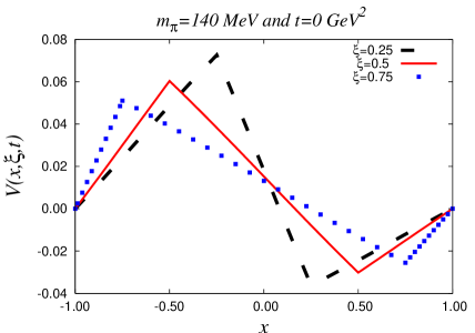
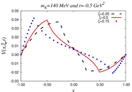
Figure 4: The vector TDA in the case $m_{\pi}=140$ MeV and, respectively, $t=0$ and $t=-0.5$ GeV².

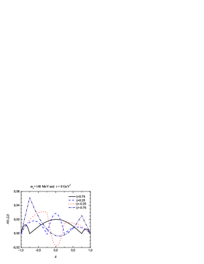
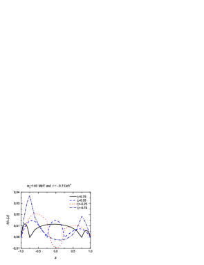
Figure 5: The axial TDA in the case $m_{\pi}=140$ MeV and, respectively, $t=0$ and $t=-0.5$ GeV².

Regarding the chiral limit, we observe that both the vector and axial TDAs do not significantly change going from a non-zero pion mass to the physical mass, except for the change in the lower bound of $\xi$.

Previous studies of pion-photon TDAs have already been done Tiburzi:2005nj ; Broniowski:2007fs . In both works, double distributions have been used. Even if our model is different, a comparison of the results is still possible. The aim of the author of the first paper Tiburzi:2005nj is to provide some estimates of the vector and axial TDAs on the basis of the positivity bounds. The order of magnitude of the obtained amplitudes are similar to ours, but the former are constrained by the $F_{V}$ and $F_{A}$ form factors, through the sum rules. The sum rules are an input imposed in Ref. Tiburzi:2005nj while it is a result in our calculation. The vector TDA obtained in this paper has some similarities with ours. Nevertheless, it does not satisfy the isospin relation (33) due to the different choice of the $u$-quark and $d$-antiquark distributions, the first one related to the pion and the second to the photon, used in the saturation of the positivity bounds. We have also studied the positivity bounds for GPDs and noticed that it is actually an upper bound that is sometimes very higher than the value of the GPD itself. The vector TDA obtained in Tiburzi:2005nj is rather peaked at $x=\pm\xi$, whereas we have a smoother behaviour.

A detailed comparison with the results of Ref. Broniowski:2007fs is not easy, due to the choice of the asymmetric notation. Nevertheless the vector TDA seems to be consistent with our results and some limits, in particular when $m_{\pi}=0$ and $t=0,$ can be recovered going from one notation to the other.

Regarding our axial TDA, it differs from the two previous calculations Tiburzi:2005nj ; Broniowski:2007fs due to the effect of the non-resonant part of the second diagram of Fig. 3. This contribution, corresponding to the last term of Eq. (23), is proportional to $\left(t-m_{\pi}^{2}\right)^{-1}$ but with zero value for the residue. The presence of this term is crucial in order to obtain the axial form factor using the sum rule. In fact, its contribution in Eq. (42) can be easily recognized. Furthermore this term is dominant in the ERBL region as we can infer from Fig. 6.

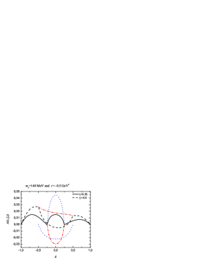
Figure 6: Contributions to the axial TDA for both positive ($\xi=0.25,$ plain line) and negative ($\xi=-0.5,$ dashed line) values of the skewness variable and for $m_{\pi}=140$ MeV and $t=-0.5$ GeV². In each case, and in the ERBL region, the contribution coming from the first diagram of Fig. 3 is represented by the dashed-dotted lines and the non-resonant part of the second diagram of Fig. 3 is represented by the dotted lines.

VI Conclusions.

In this paper we have defined the pion-photon vector and axial Transition Distribution Amplitudes using the Bethe-Salpeter amplitude for the pion. In order to make numerical predictions we have used the Nambu-Jona Lasinio model. The Pauli-Villars regularization procedure is applied in order to preserve gauge invariance.

We know from PCAC that the axial current couples to the pion. Therefore, in order to properly define the axial TDA (all the structure of the incoming hadron being included in $A\left(x,\xi,t\right)$), we need to extract the pion pole contribution. In so doing, we found that the axial TDA had two different contributions, the first one related to a direct coupling of the axial current to a quark of the incoming pion and to a quark coupled to the outcoming photon and a second related to the non-resonant part of a quark-antiquark pair coupled with the quantum numbers of the pion.

The use of a fully covariant and gauge invariant approach guaranties that we will recover all fundamental properties of the TDAs. In this way, we have the right support, $x\in\left[-1,1\right]$, and the sum rules and the polynomiality expansions are recovered. We want to stress that these three properties are not inputs, but results in our calculation. The value we found for the vector form factor in the NJL model is in agreement with the experimental result Yao:2006px whereas the value found for the axial form factor is two times larger than in Yao:2006px . This discrepancy is a common feature of quark models Broniowski:2007fs . Also the neutral pion vector form factor $F_{\pi\gamma^{\ast}\gamma}(t)$ is well described. These results allow us to assume that the NJL model gives a reasonable description of the physics of those processes at this energy regime.

Turning our attention to the polynomial expansion of the TDAs, we have seen that, in the chiral limit, only the coefficients of even powers in $\xi$ were non-null for the vector TDA. No constrain is obtained for the axial TDA. Nevertheless, the NJL model provides simple expressions for the coefficients of the polynomial expansions in the chiral limit, Eqs. (28) and (31).

We have obtained quite different shapes for the vector and axial TDAs. This is in part, at least for the DGLAP regions, imposed by the isopin relation (33). We have pointed out the importance of the non-resonant part of the qq interacting pair diagram for the axial TDA in the ERBL region.

It is interesting to inquire about the domain of validity of the relations (33). These relations are obtained from the isospin trace calculation involved in the central diagram of Fig. 3. Due to the simplicity of the isospin wave function of the pion these results are more general than the NJL model and could be considered as a result of the diagrams under consideration. These diagrams are the simplest contribution of handbag type.

The Transition Distribution Amplitudes proposed by the authors of Pire:2004ie open the possibility of enlarging the present knowledge of hadron structure for they generalize the concept of GPDs for non-diagonal transitions. Calculated here, as a first step, for pion-to-photon transitions, these new observables should lead to interesting estimates of cross section for exclusive meson pair production in $\gamma^{\ast}\gamma$ scattering Lansberg:2006fv .

Appendix A Appendix.

In Section II we have introduced the minimal kinematics definitions. The explicit expressions for the pion and photon momenta in terms of the light-front vectors are:

$$p^{\mu} =\left(1+\xi\right)\,\bar{p}^{\mu}-\frac{1}{2}\,\Delta^{\bot\mu}+\frac{1}{2}\left[P^{2}\,\left(1-\xi\right)+\frac{1}{2}\,m_{\pi}^{2}\right]\,n^{\mu}~{}~{},$$ (34)

$$p^{\prime\mu} =\left(1-\xi\right)\,\bar{p}^{\mu}+\frac{1}{2}\,\Delta^{\bot\mu}+\frac{1}{2}\left[P^{2}\,\left(1+\xi\right)-\frac{1}{2}\,m_{\pi}^{2}\right]\,n^{\mu}~{}~{}.$$ (35)

Here we have $P^{2}=\left[(p+p^{\prime})/2\right]^{2}=m_{\pi}^{2}/2-t/4,$ $\Delta^{\mu}=\left(p^{\prime}-p\right)^{\mu},$ $\Delta^{\bot\mu}=\left(0,\Delta^{1},\Delta^{2},0\right)=\left(0,\vec{\Delta}^{\bot},0\right)$ and $\Delta^{2}=t.$ The polarization vector of the real photon, $\varepsilon,$ must satisfy the transverse condition, $\varepsilon.p^{\prime}=0,$ and an additional gauge fixing condition. When deriving Eq. (5), we need $\varepsilon.n=\varepsilon^{+}/P^{+}$ to kinematically become higher-twist, i.e. $\varepsilon.n\rightarrow 0$ when $P^{+}\rightarrow\infty$. The standard gauge fixing conditions, $\varepsilon^{0}=0$ or $\varepsilon^{+}=0,$ satisfy the previous requirement. In fact, all what we need is that the components of the polarization vector remain finite when $P^{+}$ goes to infinity.

In Section III we use the NJL model. We follow the notation of Ref. Theussl:2002xp and we refer the reader to this paper for more details. The NJL model considers the lagrangian

$$\mathcal{L}=\bar{q}\left(x\right)\left(i\hbox to0.0pt{$/$\hss}\partial-\mu_{0}\right)q\left(x\right)+g\left[\left(\bar{q}q\right)^{2}+\left(\bar{q}i\gamma_{5}\vec{\tau}q\right)^{2}\right]\quad,$$ (36)

where $\mu_{0}$ is the current quark mass. As it is well known, the first consequence of the scalar interacting term is to provide a constituent quark mass, $m,$ different from the current mass. Due to the point-like character of the interaction, this lagrangian is not renormalizable. We shall use the Pauli-Villars regularization in order to render the occurring integrals finite. This means that for integrals like the ones defined in Eq. (14), we make the replacement

$$\int\frac{d^{4}p}{(2\pi)^{4}}f(p;m^{2})\longrightarrow\int\frac{d^{4}p}{(2\pi)^{4}}\sum_{j=0}^{2}c_{j}f(p;m_{j}^{2})\quad,$$ (37)

with $m_{j}^{2}=m^{2}+j\Lambda^{2}$, $c_{0}=c_{2}=1,$ $c_{1}=-2$. Following Ref. Klevansky:1992qe the regularization parameters $\Lambda$ and $m$ are determined by fitting the pion decay constant and the quark condensate (in the chiral limit). With the conventional values $\left\langle\bar{u}u\right\rangle=-(250\,\operatorname{MeV})^{3}$ and $f_{\pi}=93$ MeV, we get $m=241$ MeV and $\Lambda=859$ MeV.

The pion-quark coupling constant is given by

$$g_{\pi qq}^{2}=\frac{-1}{12\left(I_{2}\left(m_{\pi}^{2}\right)+m_{\pi}^{2}\left(\partial I_{2}\left(p\right)/\partial p^{2}\right)_{p^{2}=m_{\pi}^{2}}\right)}\quad,$$ (38)

with

$$I_{2}\left(p^{2}\right) =i\int\frac{d^{4}k}{\left(2\pi\right)^{4}}\frac{1}{\left(k^{2}-m^{2}+i\epsilon\right)\left(\left(k+p\right)^{2}-m^{2}+i\epsilon\right)}$$

$$=\frac{1}{16\pi^{2}}\sum_{j=0}^{2}c_{j}\left\{\log\frac{m_{j}^{2}}{m^{2}}+2\sqrt{\frac{4m_{j}^{2}}{p^{2}}-1}\arctan\frac{1}{\sqrt{\frac{4m_{j}^{2}}{p^{2}}-1}}\right\}.$$ (39)

The numerical value of the pion quark coupling constant is $g_{\pi qq}^{2}=6.36$ for the physical value of the mass of the $\pi^{+}$ pion, and $g_{\pi qq}^{2}=6.71$ in the chiral limit.

In the NJL model, the vector form factor is

$$F_{V}^{\pi^{+}}(t)=\frac{8\,N_{c}}{3}\,m\,m_{\pi}\,\frac{g_{\pi qq}}{\sqrt{2}}\,I_{3}(p,p^{\prime})\qquad.$$ (40)

In order to calculate the form factors we need the expression for the three-propagator integral. In the particular case where $p^{2}=m_{\pi}^{2}$ and $p^{\prime}{}^{2}=0$, the expression for $I_{3}(p,p^{\prime})$ is

$$I_{3}(p,p^{\prime}) =i\,\int\,\,\frac{d^{4}k}{(2\pi)^{4}}\,\,\frac{1}{\left(k^{2}-m^{2}+i\epsilon\right)\left((p+k)^{2}-m^{2}+i\epsilon\right)\left((p^{\prime}+k)^{2}-m^{2}+i\epsilon\right)}\qquad,$$

$$=\frac{1}{(4\pi)^{2}}\,\sum_{j=0}^{2}c_{j}\,\int_{0}^{1}dx\,\frac{x}{\sqrt{\rho}}\,\mbox{log}\,\frac{x^{2}t+x(1-x)m_{\pi}^{2}-2m_{j}^{2}-\sqrt{\rho}}{x^{2}t+x(1-x)m_{\pi}^{2}-2m_{j}^{2}+\sqrt{\rho}}\qquad,$$ (41)

with $\rho=t^{2}x^{4}+x^{2}(1-x)^{2}m_{\pi}^{4}+2\,t\,x^{2}(m_{\pi}^{2}x(1-x)-2m_{j}^{2}),~{}t=\left(p^{\prime}-p\right)^{2}$.

The axial form factor involves the three-propagator integral as well, but also the two-propagator integral given by Eq. 39

$$F_{A}^{\pi^{+}}(t)=4N_{c}\,m\,m_{\pi}\,g_{\pi qq}\sqrt{2}\,\left(I_{3}(p,p^{\prime})+\frac{2}{m_{\pi}^{2}-t}\left[I_{2}(m_{\pi}^{2})-I_{2}(t)\right]\right)\qquad,$$ (42)

The $\pi^{0}\rightarrow\gamma^{\ast}\gamma$ form factor can be obtained from the vector form factor through a isospin rotation: $F_{\pi\gamma^{\ast}\gamma}\left(t\right)=\sqrt{2}F_{V}^{\pi^{+}}\left(t\right)/m_{\pi}.$ In the chiral limit and for $t=0$ all the considered form factors have the simple expression:

$$\left.\frac{F_{\pi\gamma^{\ast}\gamma}\left(0\right)}{\sqrt{2}}\right|_{m_{\pi}\rightarrow 0} =\left.\frac{F_{V}^{\pi^{+}}\left(0\right)}{m_{\pi}}\right|_{m_{\pi}\rightarrow 0}=\left.\frac{F_{A}^{\pi^{+}}\left(0\right)}{m_{\pi}}\right|_{m_{\pi}\rightarrow 0}=\frac{1}{\sqrt{2}4\pi^{2}f_{\pi}}\left[1-\frac{2m^{2}}{m^{2}+\Lambda^{2}}+\frac{m^{2}}{m^{2}+2\Lambda^{2}}\right]$$

$$=0.192\times\left(1-0.108\right)\operatorname{GeV}^{-1}=0.171\operatorname{GeV}^{-1}$$ (43)

The first coefficient of the right hand side is what is expected from the axial anomaly contribution to $\pi\rightarrow\gamma\gamma$ decay. The term between brackets has a small correction to the expected value of 1 due to the finiteness of the regularization masses. In the NJL model not only the quarks, but also the counter-terms run in the triangle diagram of the axial anomaly.In a proper renormalizable theory this correction disappears in the limit $\Lambda\rightarrow\infty.$

In the light-front calculations we need two kind of integrals. The first one is

$$\tilde{I}_{2}\left(x,\xi,t\right) =i\int\frac{d^{4}k}{(2\pi)^{4}}\,\,\frac{\delta\left(x-1+\frac{k^{+}}{P^{+}}\right)}{[(k-p_{1})^{2}-m^{2}+i\epsilon][(k-p_{2})^{2}-m^{2}+i\epsilon]}\quad,$$

$$=\theta(b-x)\theta(x-a)\,\frac{1}{(4\pi)^{2}}\,\frac{1}{a-b}\,\sum_{j=1}^{2}c_{j}\,\mbox{log}\,\frac{m^{2}(b-a)^{2}-(b-x)(x-a)(p_{2}-p_{1})^{2}}{m_{j}^{2}(b-a)^{2}-(b-x)(x-a)(p_{2}-p_{1})^{2}}\qquad,$$ (44)

with $b=$max$\left(1-p_{1}^{+}/P^{+},1-p_{2}^{+}/P^{+}\right)$ and $a=$min$\left(1-p_{1}^{+}/P^{+},1-p_{2}^{+}/P^{+}\right)$. The second light-front integral needed in our calculations is the one defined by Eq. (14). This integral can be performed by standard methods, obtaining

$$\tilde{I}_{3v}\left(x,\xi,t\right)=\frac{1}{32\,\pi^{2}}\,\sum_{j=0}^{2}c_{j}\,\frac{1}{\sqrt{D}}\,\mbox{log}\,\frac{-\frac{t}{2}(1-x)+C+\sqrt{D}}{-\frac{t}{2}(1-x)+C-\sqrt{D}}\qquad,$$ (45)

with

$$D =\left(\frac{m_{\pi}^{2}}{2}(\xi-x)-\frac{t}{2}(1-x)\right)^{2}+m_{j}^{2}(1-\xi)\left(2m_{\pi}^{2}\xi-t(1+\xi)\right)\qquad,$$

$$C =\left\{\begin{array}[c]{ccl}\frac{m_{\pi}^{2}}{2}(\xi-x)+m_{j}^{2}\frac{(1-\xi^{2})}{(1-x)}\quad,&&|\xi|<x<1,\\ &&\\ -\frac{m_{\pi}^{2}}{2}(\xi-x)+m_{j}^{2}\frac{2\xi(1+\xi)}{(x+\xi)}\quad,&&-|\xi|<x<|\xi|~{}~{}~{}~{}~{}~{}~{}\xi>0\\ &&\\ -\frac{m_{\pi}^{2}}{2}(\xi+x)-m_{j}^{2}\frac{2\xi(1-\xi)}{(x-\xi)}\quad,&&-|\xi|<x<|\xi|~{}~{}~{}~{}~{}~{}~{}\xi<0\quad.\end{array}\right.$$ (48)

As an aplication of the expression (44) we can evaluate the PDA. From its definition in Eq. (8) we have

$$\phi\left(x\right)=-\frac{4\,N_{c}\,m\,g_{\pi qq}}{f_{\pi}}i\int\frac{d^{4}k}{(2\pi)^{4}}\,\,\frac{\delta\left(x-1+\frac{k^{+}}{p^{+}}\right)}{[k^{2}-m^{2}+i\epsilon][(k-p)^{2}-m^{2}+i\epsilon]}~{}~{}.$$ (49)

This integral is of the type of (44) with $a=0$ and $b=1.$ Therefore

$$\phi\left(x\right)=\frac{N_{c}\,m\,g_{\pi qq}}{4\,\pi^{2}\,f_{\pi}}\,\theta\left(x\right)\,\theta\left(1-x\right)\sum_{j=1}^{2}c_{j}\,\log\,\frac{m^{2}-m_{\pi}^{2}\,(1-x)\,x}{m_{j}^{2}-m_{\pi}^{2}\,(1-x)\,x}~{}~{}.$$ (50)

As it is expected for the PDA, $x$ runs from 0 to 1. We can test our result verifying that in the chiral limit $\phi\left(x\right)=\theta\left(x\right)\,\theta\left(1-x\right),$ as it is well known for the NJL model. This peculiarity of the NJL model in this limit is present also in the quark valence distribution, which becomes as simple as $q(x)=\theta\left(x\right)~{}\theta(1-x)$. In Ref. Noguera:2005cc is discussed how this is, in fact, a quite reasonable approximation of realistic models.

References

(1)R. L. Jaffe,
arXiv:hep-ph/9602236.
(2)D. Mueller, D. Robaschik, B. Geyer, F. M. Dittes and
J. Horejsi,
Fortsch. Phys. 42 (1994) 101 [arXiv:hep-ph/9812448].
(3)A. V. Radyushkin,
Phys. Lett. B 380 (1996) 417 [arXiv:hep-ph/9604317],
Phys. Lett. B 385 (1996) 333 [arXiv:hep-ph/9605431].
(4)X. D. Ji,
Phys. Rev. Lett. 78 (1997) 610
[arXiv:hep-ph/9603249],Phys. Rev. D 55 (1997) 7114
[arXiv:hep-ph/9609381].