Inverse scattering in multimode structures

Abstract

We consider the inverse scattering problem associated with any number of interacting modes in one-dimensional structures. The coupling between the modes is contradirectional in addition to codirectional, and may be distributed continuously or in discrete points. The local coupling as a function of position is obtained from reflection data using a layer-stripping type method, and the separate identification of the contradirectional and codirectional coupling is obtained using matrix factorization. Ambiguities are discussed in detail, and different a priori information that can resolve the ambiguities is suggested. The method is exemplified by applications to multimode optical waveguides with quasi-periodical perturbations.

1 Introduction

In waveguides that support several modes, scattering, or coupling between the different modes, may appear due to different kinds of perturbations. Possible perturbations are reflectors, gratings, bends, tapering, and other kind of geometrical or material modulation along the waveguide. The coupling may be both codirectional (coupling between modes that propagate in the same direction) or contradirectional (coupling between modes that propagate in opposite directions). The direct scattering problem of computing the scattered field when the probing waves and the scattering structure are known has been extensively discussed in the literature [24, 38, 21]. The inverse scattering problem associated with two interacting modes is also well understood, and has been treated in several contexts since the pioneering work by Gel’fand and Levitan [13], Marchenko [3], and Krein [22]. In geophysics the so-called dynamic deconvolution or layer-stripping (layer-peeling) methods emerged, for the identification of layered-earth models from acoustic scattering data [28, 31, 2, 6, 5]. More recently the inverse scattering methods have been applied to the design and characterization of optical devices involving two interacting modes. Both contradirectional coupling and codirectional coupling have been treated. Optical components based on contradirectional coupling include thin-film filters and fiber Bragg gratings [40, 10, 37, 30, 36, 34], while codirectional coupling is present in e.g. grating-assisted codirectional couplers and long-period gratings [19, 39, 9, 42, 4]. While the inverse-scattering problem associated with two interacting modes is well-known, the inverse-scattering problem of several, possibly non-degenerate modes (i.e., with different propagation constants) seems unsolved so far. Some work has been done in the case of 4 degenerate modes, that is, two polarization modes in each direction [35, 41], and several degenerate modes with only contradirectional coupling [1].

On the other hand, several methods for the inverse scattering of acoustic or electromagnetic waves in two or three dimensions have been reported. In particular, Yagle et al. have developed layer-stripping methods for the multidimensional case [45, 43, 44]. By Fourier transforming the problem with respect to the transversal coordinates, the multidimensional problem may be regarded as one-dimensional with several interacting modes.

In this paper we will extend these lines of thought to cover the general inverse scattering problem associated with any number of interacting modes in one-dimensional, reciprocal structures. In the model (Section 2) both codirectional and contradirectional coupling may be present simultaneously. We limit ourselves to the case where the known probing waves and the scattered waves propagate in opposite directions. In other words the scattered wave is considered as a reflection from the unknown structure. A layer-stripping inverse scattering algorithm is presented in Section 3. Ambiguities related to the simultaneous presence of co- and contradirectional coupling are discussed in detail. Possible a priori information that can resolve these ambiguities will be suggested. The formalism is particularly useful for the quasi-periodical case (Section 4), since only the slowly varying envelope needs to be represented rather than the structure itself, yielding an efficient algorithm. In Section 5, the method is applied for the numerical reconstruction of a quasi-periodical waveguide structure. Sections 4 and 5 are exemplified by a multimode fiber Bragg grating; an optical fiber with quasi-periodic refractive index perturbation along the fiber axis, giving rise to both co- and contradirectional coupling. Finally, analogies to the multidimensional case are discussed in Section 6.

2 Continuous and discrete coupling model

Consider a structure with $P$ modes propagating in each direction along the $x$-axis. We visualize the $x$-axis as being directed to the right, and say that the $+x$-direction is the forward direction. The propagation constant of the $p$th mode is $\pm\beta_{p}$, i.e., the $x$-dependence of the complex field associated with mode $p$ is described by the factor $\exp(\pm i\beta_{p}x)$, where the upper (lower) sign applies to forward (backward) propagating modes. Note that the propagation constants of different modes may or may not be different. The propagation constants are related to frequency through the dispersion relation of the structure. The propagation constants may be expressed $\beta_{p}=n_{p}\omega/c$, where $\omega$ is the angular frequency, $c$ is some fixed reference velocity (common for all modes), and $n_{p}$ accounts for the actual phase velocity. (However, in some cases it may rather be convenient to express the propagation constants in the form $n_{p}\omega/c-\pi/\Lambda$, where $\Lambda$ is a constant, see Section 4.) For electromagnetic waves, it is natural to set $c$ equal to the vacuum velocity, and consequently we will refer to $n_{p}$ as the effective index associated with mode $p$. In principle, the effective indices may be complex and dependent on frequency, meaning that modal loss and dispersion are permitted in the model. However, the dispersion must be limited by relativistic causality in the sense that any signal carried by the modes travels no faster than the vacuum light velocity. Also, the modal field profiles are assumed to have uniform phases such that they can be written real.

Coupling may occur due to a continuous or discrete scattering structure. In the first case, the field is assumed to be governed by the coupled-mode equation

$$\frac{\text{d}\mathbf{E}}{\text{d}x}=i\mathbf{C}\mathbf{E},$$ (1)

where $\mathbf{E}$ is a column vector containing the $2P$ mode amplitudes. In the absence of the scattering structure ($\mathbf{C}_{\boldsymbol{\sigma}}=\mathbf{C}_{\boldsymbol{\kappa}}=0$, see below), the first $P$ elements are the mode amplitudes of the forward propagating modes (propagating in the $+x$ direction) and the last $P$ elements are those of the backward propagating modes. The coupling matrix $\mathbf{C}$ can be decomposed into three contributions:

$$\mathbf{C}=\mathbf{D}+\mathbf{C}_{\boldsymbol{\sigma}}+\mathbf{C}_{\boldsymbol{\kappa}}.$$ (2)

The contributions can be expressed as $2\times 2$ block matrices consisting of $P\times P$ blocks:

$$\mathbf{D} =\begin{bmatrix}\boldsymbol{\beta}&\boldsymbol{0}\\ \boldsymbol{0}&-\boldsymbol{\beta}\end{bmatrix},$$ (3a)

$$\mathbf{C}_{\boldsymbol{\kappa}} =\begin{bmatrix}\boldsymbol{0}&\boldsymbol{\kappa}\\ -\boldsymbol{\kappa}^{*}&\boldsymbol{0}\end{bmatrix},$$ (3b)

$$\mathbf{C}_{\boldsymbol{\sigma}} =\begin{bmatrix}\boldsymbol{\sigma}&\boldsymbol{0}\\ \boldsymbol{0}&-\boldsymbol{\sigma}^{*}\end{bmatrix},$$ (3c)

where * denotes complex conjugate. The first term $\mathbf{D}$ describes the frequency dependence due to the propagation of the different modes (“self-coupling”), and is independent on $x$; and $\boldsymbol{\beta}=\mathop{\operator@font diag}\nolimits\{\beta_{1},\beta_{2},\ldots,\beta_{P}\}$. Only this term is permitted to be lossy in the model ($\boldsymbol{\beta}$ may be complex). In practice, we should require $\text{Im}\>\beta_{p}L\lesssim 1$, where $L$ is the total length of the structure; otherwise the field at the far end of the structure may be close to zero (i.e., the mode will be bound at the left interface to the structure, and very little reflection will originate from the far end.). The second term $\mathbf{C}_{\boldsymbol{\kappa}}$ describes the coupling between counterpropagating modes, whereas the last term $\mathbf{C}_{\boldsymbol{\sigma}}$ accounts for the coupling between copropagating modes. The coupling coefficients $\boldsymbol{\kappa}$ and $\boldsymbol{\sigma}$ are dependent on $x$ but assumed independent on frequency. As will become clear shortly, the above forms of $\mathbf{C}_{\boldsymbol{\kappa}}$ and $\mathbf{C}_{\boldsymbol{\sigma}}$ are consequences of reciprocity and losslessness. It should be noted that in structures such as long-period gratings, where the coupling is purely codirectional, the coupling is described by $\boldsymbol{\kappa}=\boldsymbol{0}$ and a $\boldsymbol{\sigma}$ with non-zero off-diagonal elements. The conventional way of describing such structures would be only to consider the upper-left $P\times P$ block of $\mathbf{C}$. The layer-stripping method in Sec. 3 cannot be used to reconstruct such structures since the reflection response is zero.

The coupling region in the waveguide is discretized into $N$ layers, each of thickness $\Delta x=L/N$. If $N$ is sufficiently large so that the matrices in (3) can be treated as constants in each layer, we can solve (1):

$$\mathbf{E}(x_{j}+\Delta x)=\exp{(i\mathbf{C}\Delta x)}\mathbf{E}(x_{j}),\quad x_{j}=j\Delta x.$$ (4)

This transfer matrix relation can be used to propagate the fields through the piecewise uniform structure. With the help of the connection between the transfer matrix and the scattering matrix (Appendix B) we can find the reflection and transmission response from the total transfer matrix, obtained as a product of the transfer matrices $\exp{(i\mathbf{C}\Delta x)}$ of each layer (direct scattering).

While direct scattering is achieved straightforwardly using the piecewise-uniform discretization, for inverse scattering it is convenient to push the discretization further, to identify the different contributions to the transfer matrix $\exp{(i\mathbf{C}\Delta x)}$. To first order in $\Delta x$, we have $\exp(i\mathbf{C}\Delta x)=\exp(i\mathbf{D}\Delta x)\exp(i\mathbf{C}_{\boldsymbol{\kappa}}\Delta x)\exp(i\mathbf{C}_{\boldsymbol{\sigma}}\Delta x)$. For a continuous structure of finite thickness, the bandwidth where the reflection spectrum is significantly different from zero is finite. Thus we need only be concerned with frequencies satisfying $|\omega|\leq\omega_{\text{b}}$ for some positive constant $\omega_{\text{b}}$. Note that this model may give entirely incorrect results for $|\omega|>\omega_{\text{b}}$. For instance, if $P=1$ the reflection spectrum calculated with the discrete model will be periodic with period $\pi c/(n_{1}\Delta x)$, while the spectrum associated with a continuous structure tends to zero for large frequencies. For inverse scattering, the reflection spectrum and therefore $\omega_{\text{b}}$ are known. Therefore, provided $\Delta x$ is chosen sufficiently small we can approximate each layer by a cascade of three sections: a section with codirectional coupling, a section with contradirectional coupling, and time-delay section. The physical implication of this factorization is that the mode-coupling appears in a discrete point within the layer rather than distributed along the whole layer. The contradirectional section may therefore be pictured as a discrete reflector. The transfer matrix of the $j$th layer becomes

$$\mathbf{T}_{j}=\mathbf{T}_{\boldsymbol{Z}}\mathbf{T}_{\boldsymbol{\rho}_{j}}\mathbf{T}_{\boldsymbol{\Phi}_{j}},$$ (5)

where

$$\mathbf{T}_{\boldsymbol{Z}} \equiv\exp(i\mathbf{D}\Delta x)=\begin{bmatrix}\boldsymbol{Z}^{-1}&\boldsymbol{0}\\ \boldsymbol{0}&\boldsymbol{Z}\end{bmatrix},\quad\boldsymbol{Z}^{-1}=\exp(i\boldsymbol{\beta}\Delta x),$$ (6a)

$$\mathbf{T}_{\boldsymbol{\rho}_{j}} \equiv\exp(i\mathbf{C}_{\boldsymbol{\kappa}}\Delta x)=\begin{bmatrix}\boldsymbol{t}_{j}^{-1*}&-\boldsymbol{t}_{j}^{-1*}\boldsymbol{\rho}_{j}^{*}\\ -\boldsymbol{t}_{j}^{-1}\boldsymbol{\rho}_{j}&\boldsymbol{t}_{j}^{-1}\end{bmatrix},\quad\begin{array}[]{l}\boldsymbol{\rho}_{j}=i\tanh[(\boldsymbol{\kappa}^{*}\boldsymbol{\kappa})^{1/2}\Delta x](\boldsymbol{\kappa}^{*}\boldsymbol{\kappa})^{-1/2}\boldsymbol{\kappa}^{*},\\ \boldsymbol{t}_{j}=\cosh[(\boldsymbol{\kappa}^{*}\boldsymbol{\kappa})^{1/2}\Delta x]^{-1},\end{array}$$ (6d)

$$\mathbf{T}_{\boldsymbol{\Phi}_{j}} \equiv\exp(i\mathbf{C}_{\boldsymbol{\sigma}}\Delta x)=\begin{bmatrix}\boldsymbol{\Phi}_{j}&\boldsymbol{0}\\ \boldsymbol{0}&\boldsymbol{\Phi}_{j}^{*}\end{bmatrix},\quad\boldsymbol{\Phi}_{j}=\exp(i\boldsymbol{\sigma}\Delta x).$$ (6e)

The form of the matrix in (6d) may for example be verified by evaluating the power series expansion of the matrix exponential. In principle, it suffices to express (6) to first order in $\Delta x$; however, the exact form is kept to emphasize the properties of each of the three sections, to ensure that each section is lossless regardless of the value of $\Delta x$, and to retain the correspondence to the discrete case (below).

We are now in the position that we can argue for the forms of the coupling matrices (3). Note that while we have permitted loss in the propagation section $\boldsymbol{Z}^{-1}$, the coupling sections are assumed lossless. Since the coupling sections also are assumed to be reciprocal, their transfer matrices satisfy (61) and (62) (Appendix B). Allowing a more general $\mathbf{C}_{\boldsymbol{\kappa}}$ by substituting $\boldsymbol{\kappa}^{*}\to\boldsymbol{\kappa}_{21}$ in the (2,1) block, and expanding $\exp(i\mathbf{C}_{\boldsymbol{\kappa}}\Delta x)$ to first order in $\Delta x$, the lossless and reciprocity conditions give $\boldsymbol{\kappa}_{12}=-\boldsymbol{\kappa}^{*}$ and dictate $\boldsymbol{\kappa}$ to be symmetric. Similarly, we can derive the form of $\mathbf{C}_{\boldsymbol{\sigma}}$ and establish that $\boldsymbol{\Phi}_{j}$ must be unitary, i.e., $\boldsymbol{\sigma}$ is hermitian.

From the discussion above, each layer is characterized by a unitary codirectional coupling matrix $\boldsymbol{\Phi}_{j}$ and a discrete reflector. Let superscript T denote transpose and let $\|\cdot\|$ be the usual matrix 2-norm. The discrete reflector satisfies $\boldsymbol{\rho}_{j}=\boldsymbol{\rho}_{j}^{\text{T}}$ and $\|\boldsymbol{\rho}_{j}\|<1$, and has an associated, positive definite transmission matrix $\boldsymbol{t}_{j}$ with $\boldsymbol{t}_{j}^{2}=\boldsymbol{I}-\boldsymbol{\rho}_{j}\boldsymbol{\rho}_{j}^{*}$.

So far we have considered a continuous scattering structure, and discretized it into a cascade of codirectional coupling, reflection, and pure propagation. Obviously, we can also describe discrete coupling directly. The most general, lossless, reciprocal coupling element can be described as a discrete reflector sandwiched between two codirectional coupling sections (Appendix B). Compared to our discrete model above, there is an extra codirectional coupling section on the right-hand side of the reflector. In the special case where all modes have equal effective index, $\boldsymbol{Z}^{-1}\propto\boldsymbol{I}$, this coupling section commutes with the delay section, and as a result it can be absorbed into the next, adjacent layer on the right-hand side. However, in the general case this extra coupling section does not commute with the delay section and cannot be ignored. For inverse scattering, this coupling section should therefore not be present since otherwise, it would not be possible to determine the transmission through the layer uniquely from the reflection. Under this assumption, $\boldsymbol{t}_{j}$ is positive semidefinite, and uniquely determined by $\boldsymbol{t}_{j}^{2}=\boldsymbol{I}-\boldsymbol{\rho}_{j}\boldsymbol{\rho}_{j}^{*}$. We restrict ourselves to reflectors that satisfy $\|\boldsymbol{\rho}_{j}\|<1$; otherwise the reflector will mask the later part of the structure such that the inverse scattering procedure will not be possible. Also, with two or more layers with $\|\boldsymbol{\rho}_{j}\|=1$, the structure may behave as an ideal resonator with bound modes.

Writing out the transfer matrix (5) of each layer, we obtain

$$\mathbf{T}_{j}=\begin{bmatrix}\boldsymbol{Z}^{-1}\boldsymbol{t}_{j}^{-1*}\boldsymbol{\Phi}_{j}&-\boldsymbol{Z}^{-1}\boldsymbol{t}_{j}^{-1*}\boldsymbol{\rho}_{j}^{*}\boldsymbol{\Phi}_{j}^{*}\\ -\boldsymbol{Z}\boldsymbol{t}_{j}^{-1}\boldsymbol{\rho}_{j}\boldsymbol{\Phi}_{j}&\boldsymbol{Z}\boldsymbol{t}_{j}^{-1}\boldsymbol{\Phi}_{j}^{*}\end{bmatrix}=\begin{bmatrix}\boldsymbol{Z}^{-1}\boldsymbol{K}_{j}&\boldsymbol{0}\\ \boldsymbol{0}&\boldsymbol{Z}\boldsymbol{K}_{j}^{*}\end{bmatrix}\begin{bmatrix}\boldsymbol{I}&-\boldsymbol{\Upsilon}_{j}^{*}\\ -\boldsymbol{\Upsilon}_{j}&\boldsymbol{I}\end{bmatrix},$$ (7)

where $\boldsymbol{\Upsilon}_{j}=\boldsymbol{\Phi}_{j}^{\text{T}}\boldsymbol{\rho}_{j}\boldsymbol{\Phi}_{j}$ and $\boldsymbol{K}_{j}=\boldsymbol{t}_{j}^{-1*}\boldsymbol{\Phi}_{j}$. The transfer matrix can be converted into a scattering matrix (Appendix B):

$$\mathbf{S}_{j}=\begin{bmatrix}\boldsymbol{\Phi}_{j}^{\text{T}}\boldsymbol{\rho}_{j}\boldsymbol{\Phi}_{j}&\boldsymbol{\Phi}_{j}^{\text{T}}\boldsymbol{t}_{j}\boldsymbol{Z}^{-1}\\ \boldsymbol{Z}^{-1}\boldsymbol{t}_{j}^{*}\boldsymbol{\Phi}_{j}&-\boldsymbol{Z}^{-1}\boldsymbol{t}_{j}^{-1*}\boldsymbol{\rho}_{j}^{*}\boldsymbol{t}_{j}\boldsymbol{Z}^{-1}\end{bmatrix}.$$ (8)

Thus, $\boldsymbol{\Upsilon}_{j}$ represents the reflection response from the left of layer $j$.

The combined transfer matrix describing the total structure with $N$ layers is given by

$${\mathbf{T}}={\mathbf{T}}_{N-1}{\mathbf{T}}_{N-2}\cdots{\mathbf{T}}_{1}{\mathbf{T}}_{0}.$$ (9)

From this matrix we can determine the reflection and transmission response using (54). For example, the reflection response from the left is

$$\boldsymbol{R}(\omega)\equiv\boldsymbol{S}_{11}=-\boldsymbol{T}_{22}^{-1}\boldsymbol{T}_{21},$$ (10)

where $\boldsymbol{T}_{kl}$ are the $P\times P$ blocks in $\mathbf{T}$. Assuming $\|\boldsymbol{\rho}_{j}\|<1$ for all $j$, it can be proven by induction that $\boldsymbol{T}_{22}$ is invertible on and above the real frequency axis in the complex $\omega$-plane, for any number of layers. Physically this is obvious since $\boldsymbol{T}_{22}^{-1}$ is the transmission response from the right, and therefore it must exist and be causal and stable.

Reciprocity (55a) gives $\boldsymbol{R}(\omega)=\boldsymbol{R}(\omega)^{\text{T}}$. Using $\|\boldsymbol{\rho}_{j}\|<1$ for all $j$, it can be shown by induction that $\|\boldsymbol{R}(\omega)\|<1$ for a passive structure (a passive structure is characterized by $\text{Im}\,\beta_{p}\geq 0$ for all $p$). By causality the reflection response can be written in the form

$$\boldsymbol{R}(\omega)=\int_{0}^{\infty}\boldsymbol{h}(t)\exp(i\omega t)\text{d}t,$$ (11)

where $\boldsymbol{h}(t)$ is called the time-domain impulse response.

When the modes are nondispersive, i.e., $\boldsymbol{\beta}$ is linearly related to frequency, $\boldsymbol{h}(t)$ equals a train of non-equally spaced, weighted delta pulses:

$$\boldsymbol{h}(t)=\sum_{k=0}^{\infty}\boldsymbol{h}^{k}\delta(t-t^{k}).$$ (12)

Here $\boldsymbol{h}^{k}$ and $t^{k}$ are the weight and arrival time of the $k$th pulse, respectively. Substituting (12) into (11) gives

$$\boldsymbol{R}(\omega)=\sum_{k=0}^{\infty}\boldsymbol{h}^{k}\exp(i\omega t^{k}).$$ (13)

The weights $\boldsymbol{h}^{k}$ can in principle be calculated from $\boldsymbol{R}(\omega)$ using an inverse transform of the form

$$\boldsymbol{h}^{k}=\lim_{\omega_{\max}\to\infty}\frac{1}{2\omega_{\max}}\int_{-\omega_{\max}}^{\omega_{\max}}\boldsymbol{R}(\omega)\exp(-i\omega t^{k})\text{d}\omega.$$ (14)

The arrival times are determined by the delay from a layer to the next of each mode. Let $\Delta t_{p}$ be the delay of mode $p$ through a single layer. A delta pulse at $t=0$ is incident to the structure on the left-hand side. Consider the reflection from the different layers, as seen from left-hand side of the structure. From layer 0, the arrival times in all modes will be zero. An impulse in mode $p$ reflected from layer 1 into mode $q$, will arrive at $\Delta t_{p}+\Delta t_{q}$. Thus, considering layer 1, the arrival times are any combinations of two unit delays $\Delta t_{p}$. Considering layer 2, the arrival times are any combinations of four unit delays, and so forth.

When the modes are dispersive, the impulse response is no longer a train of delta functions. Nevertheless, for $t=0$ it can still be written as $\boldsymbol{h}^{0}\delta(t)$, and the weight $\boldsymbol{h}^{0}$ can be found from (14).

Eq. (13) clearly demonstrate that, in principle, for a discrete structure the reflection response $\boldsymbol{R}(\omega)$ does not approach zero for large frequencies. Only in the special case where the modal effective indices are rational numbers with common denominator, the reflection spectrum is periodic. Fortunately, in practice, it is not necessary to represent the entire bandwidth to enable inverse scattering for a discrete structure. As shown in the next section, what is needed in the layer-stripping algorithm is the zeroth point of the impulse response, at time $t=0$. Since the next nonzero value is for $t=2\min_{p}\Delta t_{p}$ , the zeroth point is computed accurately provided the represented bandwidth $\omega_{\max}$ satisfies $\omega_{\max}\gg 1/\min_{p}\Delta t_{p}$. Then, if the true reflection spectrum is multiplied by a smooth window function $W(\omega)$ that goes to zero at $\omega=\pm\omega_{\max}$, the inverse Fourier transform evaluated around zero is approximately $w(t)\boldsymbol{h}^{0}$, where $w(t)$ is the inverse Fourier transform of $W(\omega)$. Since $w(0)\boldsymbol{h}^{0}\approx\frac{1}{2\pi}\int_{-\omega_{\max}}^{\omega_{\max}}W(\omega)\boldsymbol{R}(\omega)\text{d}\omega$, we can find $\boldsymbol{h}^{0}$ from a measurement of $\boldsymbol{R}(\omega)$ in the bandwidth $(-\omega_{\max},\omega_{\max})$:

$$\boldsymbol{h}^{0}\approx\frac{\int_{-\omega_{\max}}^{\omega_{\max}}W(\omega)\boldsymbol{R}(\omega)\text{d}\omega}{\int_{-\omega_{\max}}^{\omega_{\max}}W(\omega)\text{d}\omega}.$$ (15)

In many practical cases, the structure to be reconstructed is quasi-sinusoidal. More generally, the structure is often quasi-periodic, and e.g. the first “Fourier component” is to be reconstructed. In such cases, one can define modal field envelopes which vary slowly with respect to $x$ (compared to a wavelength). Similarly, one can extract slowly varying coupling coefficient envelopes. As a result, all quantities in (1) vary slowly with $x$. The relevant bandwidth in (15) will then be centered about a chosen “design frequency” rather than zero. The main advantage of this procedure is that it leads to considerably less requirements on the spatial resolution, and as a result efficient inverse scattering. This modification to the model is detailed in Section 4.

3 Layer-stripping method

The inverse scattering problem can now be stated as follows: Given a structure consisting of $N+1$ layers. Each layer consists of three sections (sublayers), the first ($\boldsymbol{\Phi}_{j}$) responsible for coupling between copropagating modes, the second ($\boldsymbol{\rho}_{j}$) responsible for coupling between counterpropagating modes, and the third a pure propagating section ($\boldsymbol{Z}^{-1}$). The propagation constants of the involved modes are known and specified in terms of $\boldsymbol{Z}^{-1}$. From a set of excitation-response pairs (that is, $\boldsymbol{R}(\omega)$), we want to reconstruct $\boldsymbol{\rho}_{j}$ and $\boldsymbol{\Phi}_{j}$ for all $j$.

The structure itself and the medium to the right are assumed to be at rest at time $t=0$. For incident waves from the left, the reflection response from the structure is described by the matrix $\boldsymbol{R}(\omega)$ of dimension $P\times P$. This matrix can be viewed as the operator which takes the excitation field vector to the reflected field vector. Its columns can be interpreted as the responses for orthonormal excitation basis vectors $\boldsymbol{e}_{1},\boldsymbol{e}_{2},\dotsc,\boldsymbol{e}_{P}$, respectively. Here $\boldsymbol{e}_{p}$ has only one nonzero element (equal to unity) at position $p$. Similarly, we can define the forward ($\boldsymbol{u}_{j}(\omega)$) and backward ($\boldsymbol{v}_{j}(\omega)$) propagating field matrices as $P\times P$ matrices where the columns are the fields for orthonormal excitations $\boldsymbol{e}_{1},\boldsymbol{e}_{2},\dotsc,\boldsymbol{e}_{P}$. A subscript $j$ is specified to emphasize that $\boldsymbol{u}_{j}(\omega)$ and $\boldsymbol{v}_{j}(\omega)$ are the fields at the beginning (left-hand side) of layer $j$. The field matrices of layer $j+1$ are related to the field matrices of layer $j$ by

$$\begin{bmatrix}\boldsymbol{u}_{j+1}(\omega)\\ \boldsymbol{v}_{j+1}(\omega)\end{bmatrix}=\mathbf{T}_{j}\begin{bmatrix}\boldsymbol{u}_{j}(\omega)\\ \boldsymbol{v}_{j}(\omega)\end{bmatrix},$$ (16)

where $\mathbf{T}_{j}$ is given by (7).

The layer-stripping algorithm is based on the simple fact that the leading edge of the impulse response is independent on later parts of the structure due to causality. Hence, one can identify the first layer of the structure, and subsequently remove its effect using the associated transfer matrix.

For layer 0, we initialize $\boldsymbol{u}_{0}(\omega)=\boldsymbol{I}$ and $\boldsymbol{v}_{0}(\omega)=\boldsymbol{R}(\omega)$. We define a local reflection spectrum $\boldsymbol{R}_{j}(\omega)=\boldsymbol{v}_{j}(\omega)\boldsymbol{u}_{j}(\omega)^{-1}$ and the associated impulse response $\boldsymbol{h}_{j}(t)$ as the response of the structure after removing the first $j-1$ layers. Similarly to the impulse response of the entire structure, $\boldsymbol{h}_{j}(t)$ contains an isolated delta function at $t=0$. Due to causality, this pulse is equal to the reflection from the zeroth layer alone. Denoting the weight of this pulse $\boldsymbol{h}^{0}_{j}$, we find from (8) that

$$\boldsymbol{h}^{0}_{j}=\boldsymbol{\Upsilon}_{j}\equiv\boldsymbol{\Phi}_{j}^{\text{T}}\boldsymbol{\rho}_{j}\boldsymbol{\Phi}_{j}.$$ (17)

Note that $\boldsymbol{R}_{j}(\omega)$ is symmetric for all $\omega$ as a result of reciprocity; thus $\boldsymbol{h}^{0}_{j}$ is symmetric as well. Writing out (16) and (7), and substituting $\boldsymbol{v}_{j}(\omega)=\boldsymbol{R}_{j}(\omega)\boldsymbol{u}_{j}(\omega)$, we obtain

$$\boldsymbol{u}_{j+1}(\omega) =\boldsymbol{Z}^{-1}\boldsymbol{K}_{j}\left[\boldsymbol{I}-\boldsymbol{\Upsilon}_{j}^{*}\boldsymbol{R}_{j}(\omega)\right]\boldsymbol{u}_{j}(\omega),$$ (18a)

$$\boldsymbol{v}_{j+1}(\omega) =\boldsymbol{Z}\boldsymbol{K}^{*}_{j}\left[\boldsymbol{R}_{j}(\omega)-\boldsymbol{\Upsilon}_{j}\right]\boldsymbol{u}_{j}(\omega),$$ (18b)

and therefore

$$\boldsymbol{R}_{j+1}(\omega)=\boldsymbol{Z}\boldsymbol{K}^{*}_{j}\left[\boldsymbol{R}_{j}(\omega)-\boldsymbol{\Upsilon}_{j}\right]\left[\boldsymbol{I}-\boldsymbol{\Upsilon}_{j}^{*}\boldsymbol{R}_{j}(\omega)\right]^{-1}\boldsymbol{K}_{j}^{-1}\boldsymbol{Z}.$$ (19)

Provided $\boldsymbol{\Upsilon}_{j}$ and $\boldsymbol{K}_{j}$ are known, (19) shows that the local reflection spectrum of layer $j+1$ can be calculated directly from the local reflection spectrum of layer $j$ without calculating the fields $\boldsymbol{u}_{j+1}$ and $\boldsymbol{v}_{j+1}$. Note the similarity to the Schur formula used in scalar layer-stripping [6].

To characterize layer $j$ completely, and to identify $\boldsymbol{K}_{j}$, we must determine $\boldsymbol{\rho}_{j}$ and $\boldsymbol{\Phi}_{j}$. By counting the available degrees of freedom (in $\boldsymbol{\Upsilon}_{j}$), we immediately find that this cannot be done uniquely. It is therefore necessary to use a priori information on $\boldsymbol{\rho}_{j}$ and/or $\boldsymbol{\Phi}_{j}$. The available information may vary from situation to situation. Here we will consider the following situations, where $\boldsymbol{\rho}_{j}$ and $\boldsymbol{\Phi}_{j}$ can be found using the methods in the Appendices A.1 and A.2.

1. $\boldsymbol{\Phi}_{j}=\boldsymbol{I}$. In this case there is no codirectional coupling. The identification of the layer is now particularly simple, as $\boldsymbol{\rho}_{j}=\boldsymbol{\Upsilon}_{j}$ uniquely. Note that while there is no codirectional coupling, $\boldsymbol{\rho}_{j}$ describes reflection from all modes into all modes. Thus the different modes may still interact.

2. $\boldsymbol{\rho}_{j}$ is diagonal and nonnegative. Now $\boldsymbol{\rho}_{j}$ is a simple partial reflector which only reflects light into the same mode as the incident field (no reflection into other modes). The coupling between different modes is instead described by $\boldsymbol{\Phi}_{j}$. Since $\boldsymbol{\Upsilon}_{j}=\boldsymbol{\Phi}_{j}^{\text{T}}\boldsymbol{\rho}_{j}\boldsymbol{\Phi}_{j}$, $\boldsymbol{\rho}_{j}$ is found uniquely as the singular value matrix associated with $\boldsymbol{\Upsilon}_{j}$, up to reordering of the singular values. Once the order of the singular values has been established, the unitary $\boldsymbol{\Phi}_{j}$ is found uniquely up to the sign of its rows, provided all singular values are distinct and nonzero (see Appendix A.1). When one or more singular values of $\boldsymbol{\Upsilon}_{j}$ are zero, the corresponding row(s) of $\boldsymbol{\Phi}_{j}$ cannot be determined uniquely. More precisely, $\boldsymbol{\Phi}_{j}$ is determined up to a premultiplicative unitary matrix $\boldsymbol{J}$ operating on the associated mode(s). Physically, this is obvious since when a singular value is zero, the associated mode is not reflected from the layer. When two or more nonvanishing singular values are equal, $\boldsymbol{\Phi}_{j}$ is determined up to a premultiplicative, real unitary $\boldsymbol{J}$ operating on the associated modes. Physically, this means that these modes experience the same reflection and thus an arbitrary (real) “rotation” of the modes is not detected. In such cases, the unitary section $\boldsymbol{\Phi}_{j}$, as determined by the method in Appendix A.1, does not necessarily correspond to the physical section. This error will propagate to the next layers according to (19).

3. $\boldsymbol{\Phi}_{j}$ is symmetric and $\boldsymbol{\rho}_{j}$ is real and positive semidefinite. A special case in which there are only two degenerate modes in each direction is treated in [41]. The reflector matrix $\boldsymbol{\rho}_{j}$ can be written $\boldsymbol{P}_{j}^{\text{T}}\boldsymbol{\Sigma}_{j}\boldsymbol{P}_{j}$, where $\boldsymbol{P}_{j}$ is a real, special unitary matrix and $\boldsymbol{\Sigma}_{j}$ is diagonal and nonnegative. Since $\boldsymbol{\Upsilon}_{j}=\boldsymbol{\Phi}_{j}^{\text{T}}\boldsymbol{\rho}_{j}\boldsymbol{\Phi}_{j}=\boldsymbol{\Phi}_{j}^{\text{T}}\boldsymbol{P}_{j}^{\text{T}}\boldsymbol{\Sigma}_{j}\boldsymbol{P}_{j}\boldsymbol{\Phi}_{j}$, we find $\boldsymbol{\Sigma}_{j}$ and $\boldsymbol{P}_{j}\boldsymbol{\Phi}_{j}$ as in the previous case, with the identical ambiguity issues. The separate identification of $\boldsymbol{P}_{j}$ and $\boldsymbol{\Phi}_{j}$ is accomplished using the factorization method in Appendix A.2, with certain ambiguities related to the sign of the eigenvalues of $\boldsymbol{\Phi}_{j}$.

The ambiguities when determining $\boldsymbol{\Phi}_{j}$ in situation b) are in fact very similar to the well-known ambiguities in the scalar case with a single mode in each direction. In the scalar case any $\pi$ phase-shift sections between the reflectors cannot be identified since the associated round-trip phase accumulated to and from a reflector becomes $2\pi$. In our multimode case, the sign of the rows of the “phase-delay” section ($\boldsymbol{\Phi}_{j}$) between two reflectors cannot be identified. Similarly, in the scalar case, any phase-shift section preceeding a zero reflector cannot be determined uniquely. Instead it is chosen arbitrarily (e.g. removed), and attributed to the next layer with a nonzero reflector.

When the structure to be reconstructed is a discretized version of a smooth structure, the smoothness can be used to resolve ambiguites. First we consider situation b). For small $\Delta x$, $\boldsymbol{\Phi}_{j}$ is close to identity; thus the sign of the rows of $\boldsymbol{\Phi}_{j}$ can be determined uniquely. If $\boldsymbol{\rho}_{j}$ has distinct eigenvalues, valid for all $j$, the order of the eigenvalues of $\boldsymbol{\rho}_{j}$ can be determined from the order of the eigenvalues of $\boldsymbol{\rho}_{j-1}$ using the smoothness of $\boldsymbol{\kappa}=\boldsymbol{\kappa}(x)$. If there are equal eigenvalues for a certain reflector $\boldsymbol{\rho}_{j}$, or if $\boldsymbol{\rho}_{j}$ is singular, the ambiguities of $\boldsymbol{\Phi}_{j}$ are characterized by the premultiplicative $\boldsymbol{J}$ matrix (Appendix A.1). In other words, the chosen $\boldsymbol{\Phi}_{j}$ is related to the corresponding true matrix ($\boldsymbol{\Phi}_{j,\text{true}}$) by $\boldsymbol{\Phi}_{j}=\boldsymbol{J}\boldsymbol{\Phi}_{j,\text{true}}$. By choosing $\boldsymbol{J}$ such that $\|\boldsymbol{\Phi}_{j}-\boldsymbol{\Phi}_{j-1}\|$ is minimum, the resulting $\boldsymbol{J}$ is close to identity (that is, $\|\boldsymbol{J}-\boldsymbol{I}\|\leq 2\|\boldsymbol{\Phi}_{j,\text{true}}-\boldsymbol{\Phi}_{j-1}\|$). Since $\boldsymbol{t}_{j}$ and $\boldsymbol{Z}^{-1}$ are close to identity as well, the order of three sections $\boldsymbol{J}$, $\boldsymbol{t}_{j}$, and $\boldsymbol{Z}^{-1}$ can be interchanged (see Section 2). Thus the error due to wrong choice of $\boldsymbol{\Phi}_{j}$ can be absorbed into $\boldsymbol{\Phi}_{j+1}$. More generally, provided only a few neighboring layers have singular or degenerate $\boldsymbol{\rho}_{j}$’s, only the corresponding and following $\boldsymbol{\Phi}_{j}$ sections may be determined erroneously, and the determination of the later part of the structure is (approximately) unaffected.

In situation c), the order of eigenvalues of $\boldsymbol{\rho}_{j}$ can be determined as in situation b). However, $\boldsymbol{P}_{j}\boldsymbol{\Phi}_{j}$ is not necessarily close to identity. Nevertheless, the sign of its rows can be determined from $\boldsymbol{P}_{j-1}\boldsymbol{\Phi}_{j-1}$ if $\boldsymbol{\kappa}=\boldsymbol{\kappa}(x)$ is sufficiently smooth. (Recall that $\boldsymbol{P}_{j}\boldsymbol{\Phi}_{j}$ is unitary, which means that in each row there exists at least one element of magnitude $\geq 1/\sqrt{P}$.) Finally, since $\boldsymbol{\Phi}_{j}$ is close to identity, its eigenvalues are close to unity. It follows that the factorization of $\boldsymbol{P}_{j}\boldsymbol{\Phi}_{j}$ into $\boldsymbol{P}_{j}$ and $\boldsymbol{\Phi}_{j}$ is unique (Appendix A.2).

From the discussion above, we summarize the layer-stripping algorithm, analogously to the scalar version described in ref. [6, 5], that can be applied to identify a structure supporting multiple modes:

1. Initialize $j=0$. Set $\boldsymbol{R}_{j}(\omega)=\boldsymbol{R}(\omega)$.

2. Compute the zeroth weight $\boldsymbol{h}_{j}^{0}$ of the impulse response. In practice this is achieved by the substitutions $\boldsymbol{h}^{0}\to\boldsymbol{h}^{0}_{j}$ and $\boldsymbol{R}(\omega)\to\boldsymbol{R}_{j}(\omega)$ in (15).

3. Use a model-specific factorization of $\boldsymbol{h}_{j}^{0}=\boldsymbol{\Phi}_{j}^{\text{T}}\boldsymbol{\rho}_{j}\boldsymbol{\Phi}_{j}$ to find $\boldsymbol{\Phi}_{j}$ and $\boldsymbol{\rho}_{j}$.

4. Calculate $\boldsymbol{t}_{j}=(\boldsymbol{I}-\boldsymbol{\rho}_{j}\boldsymbol{\rho}_{j}^{*})^{1/2}$ such that the associated eigenvalues are positive, and set $\boldsymbol{K}_{j}=\boldsymbol{t}_{j}^{-1}\boldsymbol{\Phi}_{j}$.

5. Calculate the next, local reflection response $\boldsymbol{R}_{j+1}(\omega)$ using (19).

6. If $j<N-1$, increase $j$ and return to 2.

When the scattering structure is continuous, one can use the true reflection spectrum as input to the layer-stripping algorithm, even though the structure is modelled discrete. This can be justified as follows: The layer thickness $\Delta x$ is chosen small such that the first order approximations of $\exp(i\mathbf{C}_{\boldsymbol{\kappa}}\Delta x)$ and $\exp(i\mathbf{C}_{\boldsymbol{\sigma}}\Delta x)$ are accurate. (Thus an upper bound on $\|\mathbf{C}_{\boldsymbol{\kappa}}\|$ and $\|\mathbf{C}_{\boldsymbol{\sigma}}\|$ should be known a priori.) Let $\omega\leq\omega_{\text{b}}$ be the bandwidth where the true reflection spectrum is significantly different from zero. For sufficiently small $\Delta x$, the first order approximation of $\exp(i\mathbf{D}\Delta x)$ is valid, and the true reflection spectrum is approximately equal to that of the corresponding discrete model in the bandwidth $\omega\leq\omega_{\text{b}}$. In the limit $t\to 0^{+}$, the $(p,q)$ element of the impulse response of the continuous structure can be calculated exactly from (1) using the Born approximation, yielding

$$h_{pq}(t=0^{+})\equiv\frac{1}{2\pi}\lim_{t\to 0^{+}}\int_{-\infty}^{\infty}R_{pq}(\omega)\exp(-i\omega t)\text{d}\omega=i\kappa_{pq}^{*}(x=0^{+})c/(n_{p}+n_{q}).$$ (20)

Here $\kappa_{pq}(x=0^{+})$ is the $(p,q)$ element of $\boldsymbol{\kappa}(x)$ at $x=0^{+}$. For practical computations, the integral in Eq. (20) must be truncated at $\pm\omega_{\text{b}}$; thus, to find the leading edge of $h_{pq}(t)$, one can take $t=0$ in the integral, and multiply the result by a factor of two. (Recall that by causality $\lim_{t\to 0^{-}}h_{pq}(t)=0$.) Once $\boldsymbol{\kappa}$ for the zeroth layer is found, one can propagate the fields using (19). Since we have not identified the codirectional coupling $\boldsymbol{\Phi}_{0}$ of the zeroth layer, $\boldsymbol{\Phi}_{0}$ is associated with the next layer. Thus, after the zeroth layer has been stripped off, the leading edge of the impulse response of the remaining structure becomes

$$\boldsymbol{\Phi}_{0}^{\text{T}}\left[i\kappa_{pq}^{*}(x=\Delta x^{+})c/(n_{p}+n_{q})\right]\boldsymbol{\Phi}_{0},$$ (21)

where the square bracket denotes a matrix formed by the elements inside. The identification of $\boldsymbol{\Phi}_{0}$ and $\left[i\kappa_{pq}^{*}/(n_{p}+n_{q})\right]$ can now be accomplished using the factorization methods described above. The algorithm continues in the same way, until finally the bandwidth of the reflection spectrum of the remaining structure exceeds $\omega_{\text{b}}$. This remaining part of the structure can be made arbitrarily thin by choosing a sufficiently small $\Delta x$.

The difference between the latter “quasi-continuous” formulation and the discrete algorithm is essentially the factor $n_{p}+n_{q}$, and the method for evaluating the leading edge or first point of the impulse response. When the effective indices can be approximated by some number $n_{0}$ for all $p$, $n_{p}\approx n_{0}$, one can in fact use the discrete algorithm directly: A periodic extension of the true reflection spectrum outside a principal bandwidth $[-\omega_{\text{max}},\omega_{\text{max}}]$ corresponds then to a discrete model with $\Delta x=\pi c/(2n_{0}\omega_{\text{max}})$. The first point of the impulse response is calculated by (15) using a rectangular window function $W(\omega)$. For a broad class of waveguides of practical interest, the effective indices are similar (see Section 4). While the phase relation between the modes, as described by $\boldsymbol{Z}^{-1}$, may still result in a nontrivial multimode coupling, the discrete algorithm gives accurate results. The errors due to this periodic spectrum approximation can be corrected to some extent by including the factor $(n_{p}+n_{q})/(2n_{0})$ in the elements on the right-hand side of (15). This can be justified e.g. using the Born approximation.

4 Quasi-sinusoidal coupling structures

Continuous coupling in acoustical, radio frequency, or optical waveguides may be obtained by perturbation of the effective indices $n_{p}$ associated with each mode. This can be achieved by modulation of the wall profile or waveguide medium properties. As a concrete example, we will discuss fiber Bragg gratings [17], which have attracted large interest recently due to their applications in fiber optical communications and sensors. A fiber grating is formed in an optical fiber by modulating the refractive index of the core periodically or quasi-periodically. The main peak of the reflection spectrum appears for the frequency where the reflection from a crest in the index modulation is in phase with the next reflection. Permanent gratings are fabricated by UV-illumination. In fibers doped with certain dopants such as germanium, the UV-illumination will permanently rise the refractive index of the core. Advanced fabrication methods have made it possible to manufacture complex gratings with varying index modulation amplitude and period. The layer-stripping algorithm is the most widely used method for designing the index profile to obtain a given reflection spectrum [10, 37, 36].

In most cases, the fiber grating is formed in a single-mode fiber, and coupling is only considered between the forward-propagating and backward-propagating fundamental mode. The field matrices $\boldsymbol{u}_{j}(\omega)$ and $\boldsymbol{v}_{j}(\omega)$ are then scalar functions. However, in some cases it is not sufficient to consider only one forward-propagating mode and one backward-propagating mode. For instance, a single mode fiber is always slightly birefringent, and the photosensitivity can be polarization-dependent [16]. In this case, two forward-propagating and two backward-propagating polarization modes must be considered. An inverse scattering algorithm that takes into account polarization mode coupling is described in [41]. The coupling between the two polarization modes are described by Jones matrices [20]. Both polarization modes have approximately the same effective index, so $\boldsymbol{Z}^{-1}=\exp(i\beta\Delta x)\boldsymbol{I}$, where the common propagation constant $\beta$ is scalar.

In a multi-mode fiber, the modulation of the refractive index may result in coupling between the fundamental mode and other modes. Each mode has a transversal field profile $\Psi_{p}(r,\phi)$ which is a solution to the scalar wave equation in polar coordinates $r$ and $\phi$ [38]:

$$\left\{\nabla_{\text{t}}^{2}+k^{2}(\bar{n}^{2}(r)-n_{p}^{2})\right\}\Psi_{p}(r,\phi)=0.$$ (22)

Here $\bar{n}(r)$ is the unperturbed, refractive index profile of the fiber, which is assumed to be real, $\nabla_{\text{t}}$ is the transversal nabla operator, and $k=\omega/c$. The field $\Psi_{p}(r,\phi)$ and its first derivatives are continuous. For bound modes, the fields are real and orthonormal such that $\int_{A_{\infty}}\Psi_{p}(r,\phi)\Psi_{q}(r,\phi)\text{d}A=\delta(p-q)$, where $\delta(p-q)$ denotes the Kronecker delta, and $A_{\infty}$ is the entire transversal plane. The effective indices $n_{p}$ are eigenvalue solutions to (22). A mode $p$ is bound when $n_{\text{cl}}<n_{p}\leq n_{\text{co}}$, where $n_{\text{co}}$ and $n_{\text{cl}}$ are the refractive indices of the fiber core and cladding, respectively. Ignoring radiation modes, which in the vicinity of the core decay rapidly away from the excitation source, the total electric field $E(r,\phi,x)$ can be written as a superposition of forward- and backward-propagating bound modes:

$$E(r,\phi,x)=\sum_{p=1}^{P}(b_{p}^{+}(x)+b_{p}^{-}(x))\Psi_{p}(r,\phi).$$ (23)

Here $b_{p}^{\pm}(x)$ contain all $x$-dependence including the harmonic propagation factor $\exp(\pm i\beta_{p}x)$, where $\beta_{p}=kn_{p}$.

Coupling between the modes originates from longitudinal modulation of the refractive index. Let the refractive index be perturbed quasi-periodically with a spatial period $\Lambda$,

$$n(r,\phi,x)=\bar{n}(r)+\Delta n_{\text{ac}}(r,\phi,x)\cos\left(\frac{2\pi}{\Lambda}x+\theta(x)\right)+\Delta n_{\text{dc}}(r,\phi,x),$$ (24)

where $\Delta n_{\text{ac}}(r,\phi,x)$, $\Delta n_{\text{dc}}(r,\phi,x)$, and $\theta(x)$ are slowly varying with $x$ over a distance $\Lambda$. We assume that $\Delta n_{\text{ac}}(r,\phi,x)\ll\bar{n}$, and $\Delta n_{\text{dc}}(r,\phi,x)\ll\bar{n}$, which is the case for practical fiber gratings. The total electric field must satisfy the scalar wave-equation for the perturbed fiber, i.e.,

$$\left\{\nabla_{\text{t}}^{2}+\frac{\partial^{2}}{\partial x^{2}}+k^{2}n^{2}(r,\phi,x)\right\}E(r,\phi,x)=0.$$ (25)

We now substitute (23) into (25), take (22) into account, and multiply the resulting equation by $\Psi_{q}(r,\phi)$. By integration over the entire transversal plane, and recalling that the modes are orthonormal, the resulting set of second order differential equations can be decomposed into first order coupled mode equations [38],

$$\frac{\text{d}b_{p}^{+}(x)}{\text{d}x}-i\beta_{p}b_{p}^{+}(x) =i\sum_{q=1}^{P}\mathcal{C}_{pq}(x)(b_{q}^{+}(x)+b_{q}^{-}(x)),$$ (26a)

$$\frac{\text{d}b_{p}^{-}(x)}{\text{d}x}+i\beta_{p}b_{p}^{-}(x) =-i\sum_{q=1}^{P}\mathcal{C}_{pq}(x)(b_{q}^{+}(x)+b_{q}^{-}(x)),$$ (26b)

where

$$\mathcal{C}_{pq}(x)=\frac{k}{2n_{p}}\int_{A_{\infty}}(n^{2}(r,\phi,x)-\bar{n}^{2}(r))\Psi_{p}(r,\phi)\Psi_{q}(r,\phi)\text{d}A.$$ (27)

Note that the frequency-dependence of (27) can be ignored in practice, since the normalized bandwidth of interest is usually much less than unity, and the field profiles and effective indices are approximately constant in this bandwidth. Also note that since the fiber is assumed to be weakly guiding, $n_{p}$ can be set equal to $n_{\text{co}}$; thus $\mathcal{C}_{pq}=\mathcal{C}_{qp}$.

In the case of a quasi-periodic structure it is natural to write the coupling coefficient as a quasi-Fourier series:

$$\begin{split}\mathcal{C}_{pq}(x)&=\sigma_{pq}(x)+\kappa_{pq}(x)\exp\left(i\frac{2\pi}{\Lambda}x\right)+\kappa^{*}_{pq}(x)\exp\left(-i\frac{2\pi}{\Lambda}x\right)\\ &+\sum_{|m|\geq 2}\kappa^{(m)}_{pq}(x)\exp\left(i\frac{2\pi m}{\Lambda}x\right),\end{split}$$ (28)

where the “Fourier coefficients” $\kappa_{pq}(x)$, $\sigma_{pq}(x)$, and $\kappa^{(m)}_{pq}(x)$ are slowly varying over a period $\Lambda$. For a fiber grating the index modulation $n(r,\phi,x)-\bar{n}(r)$ is given by (24) and is small compared to $\bar{n}(r)$, so the zeroth and first order Fourier components dominate. Note that $\arg\{\kappa_{pq}(x)\}=\theta(x)$.

The field amplitudes $b_{p}^{\pm}(x)$ vary rapidly; it is therefore convenient to introduce the slowly varying field envelopes $u_{p}(x)$ and $v_{p}(x)$ by setting

$$b_{p}^{+}(x) =i^{1/2}u_{p}(x)\exp\left(i\frac{\pi}{\Lambda}x\right)\exp\left(i\frac{\theta(x)}{2}\right),$$ (29a)

$$b_{p}^{-}(x) =i^{-1/2}v_{p}(x)\exp\left(-i\frac{\pi}{\Lambda}x\right)\exp\left(-i\frac{\theta(x)}{2}\right).$$ (29b)

Since an identical phase factor is removed from all modes, the reflection response as calculated from $b_{p}^{+}$ and $b_{q}^{-}$ will only differ from that calculated from $u_{p}$ and $v_{q}$ by a constant phase factor not dependent on $p$ and $q$. Inserting (28) and (29) into (26), and ignoring rapidly oscillating terms (since they contribute little to $\text{d}u_{p}/\text{d}x$ and $\text{d}v_{p}/\text{d}x$), we obtain an alternative set of coupled-mode equations

$$\frac{\text{d}u_{p}(x)}{\text{d}x} =i\delta_{p}u_{p}(x)-\frac{i}{2}\frac{\text{d}\theta(x)}{\text{d}x}u_{p}(x)+i\sum_{q=1}^{P}\sigma_{pq}(x)u_{q}(x)+\sum_{q=1}^{P}|\kappa_{pq}(x)|v_{q}(x),$$ (30a)

$$\frac{\text{d}v_{p}(x)}{\text{d}x} =-i\delta_{p}v_{p}(x)+\frac{i}{2}\frac{\text{d}\theta(x)}{\text{d}x}v_{p}(x)-i\sum_{q=1}^{P}\sigma_{pq}(x)v_{q}(x)+\sum_{q=1}^{P}|\kappa_{pq}(x)|u_{q}(x),$$ (30b)

where $\delta_{p}=\beta_{p}-\pi/\Lambda=n_{p}\omega/c-\pi/\Lambda$ is the wavenumber detuning of mode $p$. Thus, $-i|\kappa_{pq}(x)|$ is the coupling coefficient between modes $p$ and $q$ propagating in opposite directions, while $\sigma_{pq}(x)-\delta(p-q)(\text{d}\theta(x)/\text{d}x)/2$ is the coupling coefficient between modes $p$ and $q$ in the same direction. With $\boldsymbol{E}=[u_{1},u_{2},\ldots,u_{P},v_{1},v_{2},\ldots,v_{P}]^{\text{T}}$ we find that (30) coincides with (1), where $\sigma_{pq}(x)-\delta(p-q)(\text{d}\theta(x)/\text{d}x)/2$ and $-i|\kappa_{pq}(x)|$ are the $(p,q)$ elements of $\boldsymbol{\sigma}$ and $\boldsymbol{\kappa}$, respectively, and $\delta_{p}$ are the diagonal elements of $\boldsymbol{\beta}$. Note that $\delta_{p}$ do not correspond to the actual propagation constants but rather their detuning from $\pi/\Lambda$. Approximating the effective indices by $n_{\text{co}}$, this means that the bandwidth of interest is not centered about zero but rather about the “design frequency” $\omega_{0}\equiv\pi c/(n_{\text{co}}\Lambda)$. The frequency interval of integration in (15) should be centered about $\omega_{0}$. As in the scalar case [36], we also note that in general, the geometrical phase variation $\theta(x)$ cannot be distinguished from the phase variation associated with the dc index term $\Delta n_{\text{dc}}(r,\phi,x)$.

We observe that $\boldsymbol{\sigma}$ is real and symmetric, and $\boldsymbol{\kappa}$ is imaginary and symmetric. Moreover, it is not difficult to realize that $i\boldsymbol{\kappa}$ is positive semidefinite. Thus $\boldsymbol{\Phi}_{j}$ defined in (6) is unitary and symmetric, and $-\boldsymbol{\rho}_{j}$ is real and positive semidefinite. It follows that we can use the layer-stripping method together with the factorization approach c), as given in Section 3, to identify the coupling sections $\boldsymbol{\rho}_{j}$ and $\boldsymbol{\Phi}_{j}$ (and therefore the coupling matrices $\boldsymbol{\kappa}$ and $\boldsymbol{\sigma}$ as a function of position $x$). Since $(i\boldsymbol{\Phi}_{j})^{\text{T}}(-\boldsymbol{\rho}_{j})(i\boldsymbol{\Phi}_{j})=\boldsymbol{\Phi}_{j}^{\text{T}}\boldsymbol{\rho}_{j}\boldsymbol{\Phi}_{j}$, the factorization approach gives $-\boldsymbol{\rho}_{j}$ and $i\boldsymbol{\Phi}_{j}$.

For a fiber grating it is usually reasonable to assume that the ac and dc index modulations can be written in the forms $\Delta n_{\text{ac}}(r,\phi,x)=\Delta n(r,\phi)\Delta n_{\text{ac}}(x)$ and $\Delta n_{\text{dc}}(r,\phi,x)=\Delta n(r,\phi)\Delta n_{\text{dc}}(x)$, respectively. Here $\Delta n(r,\phi)$ accounts for the transversal variation of the index modulation profile, and $\Delta n_{\text{ac}}(x)$ and $\Delta n_{\text{dc}}(x)$ are the ac and dc modulations as a function of $x$. As before, we assume that the index modulation and $n_{\text{co}}-n_{\text{cl}}$ are small, yielding

$$\boldsymbol{\kappa}(x) =-i\frac{\Delta n_{\text{ac}}(x)}{2}\boldsymbol{\eta},$$ (31a)

$$\boldsymbol{\sigma}(x) =\Delta n_{\text{dc}}(x)\boldsymbol{\eta}-\frac{1}{2}\frac{\text{d}\theta(x)}{\text{d}x}\boldsymbol{I},$$ (31b)

where $\boldsymbol{\eta}$ is independent on $x$. The elements of $\boldsymbol{\eta}$ are

$$\eta_{pq}=k\int_{A_{\infty}}\Delta n(r,\phi)\Psi_{p}\Psi_{q}\text{d}A.$$ (32)

When the mode profiles and $\Delta n(r,\phi)$ are known, this means that the entire coupling matrix $\boldsymbol{\kappa}(x)$ is determined from only a single nonvanishing element. For $\boldsymbol{\sigma}$, two elements are needed (including at least one diagonal element). Note that in this case, it is indeed possible to distinguish between the dc index modulation $\Delta n_{\text{dc}}(x)$ and the geometrical phase variation $\text{d}\theta(x)/\text{d}x$ using information contained in $\boldsymbol{\sigma}$.

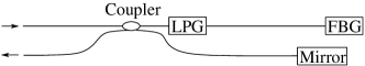
For characterization of multimode gratings, measurements of the reflection from every mode to every mode are required. Performing such measurements is not trivial. In Ref. [33], an auxiliary long-period grating (LPG), i.e, a grating with purely codirectional coupling, is used to characterize another interrogated LPG. Fig. 1 shows how this method can be adopted to characterization of multimode fiber Bragg gratings (FBGs) using optical frequency domain reflectometry [12], provided there are no degenerated modes. Light is coupled into the fundamental mode of the input fiber and the frequency of the highly coherent source is swept. The coupler splits the light equally into two fibers. The LPG couples light from the fundamental modes into the other modes so that the total optical power is distributed between all modes. The light returned by the FBG will again propagate through the LPG, and some light from each mode will be coupled back into the fundamental mode. The mirror reflects only the fundamental mode, and at the coupler the reflected light from the mirror interferes with the light in the fundamental mode out of the LPG. If the fiber between the LPG and FBG is sufficiently long such that the difference in delay between the modes is larger than the length of the impulse response of the FBG, the individual elements of the reflection matrix will be separable in the time-domain.

Fig. 1: Measurement setup for characterization of multimode gratings.

5 Numerical example

A potential application of the multimode layer-stripping method is to characterize coupling from the core mode to cladding modes in a single mode fiber. Cladding modes are not bound within the core of the fiber, but by the cladding/air boundary [8]. A single mode fiber may support as many as 100 cladding modes. The power in these modes will eventually be lost to the environment. The core-cladding mode coupling can be seen clearly in the transmission spectra of strong gratings. For chirped gratings [26] and chirped, sampled gratings [27], the bandwidth may become larger than the separation in resonant wavelength between the core-core mode coupling and the core-cladding mode coupling. Then the core-cladding mode coupling will interfere with the reflection spectrum associated with the core mode [11]. This unwanted coupling is often handled by writing the grating in fibers with depressed cladding modes [7]. There has also been some attempts of taking into account the core-cladding mode coupling in the design of the grating [23, 14]. Here, direct scattering is treated with multiple mode coupling, but the inverse scattering has so far been purely single-mode. The layer-stripping algorithm described in Section 3 can be used for characterization of such coupling and possibly for design. In contrast to the methods in [23, 14], multiple modes can be taken into account in the inverse scattering part of an iterative design process.

A simpler, but nevertheless interesting problem is to characterize coupling in an optical fiber with a few bound modes. Here, we will present a numerical experiment simulating a grating in a fiber with $n_{\text{co}}=1.452$, $n_{\text{cl}}=1.437$, and core radius $r_{\text{co}}=5\>\mu$m. By solving the eigenvalue equation for a circular fiber [38], we find that this fiber supports four modes: LP₀₁, LP₁₁, LP₂₁, and LP₀₂ at the design wavelength $\lambda_{0}=$ 1.55 $\mu$m. Here, the index $l$ in LP_lm means that the transversal field profile can be written in the form $f_{lm}(r)\cos(l\phi)$. In the further discussion, these modes are denoted 1 to 4 in the order indicated above. The eigenvalue equation gives the modal indices $n_{1}$=1.449, $n_{2}$=1.444, $n_{3}$=1.439, and $n_{4}$=1.437. We assume that the refractive index is modulated uniformly in the core of the fiber, but not at all in the cladding. This is quite realistic since, during fabrication, the fiber usually is made sensitive to UV exposure only in the core. By evaluating (32), we find that there will be no coupling between modes with different azimuthal indices $l$:

$$\boldsymbol{\eta}=\frac{2\pi}{\lambda_{0}}\begin{bmatrix}0.957&0&0&-0.116\\ 0&0.874&0&0\\ 0&0&0.707&0\\ -0.116&0&0&0.491\end{bmatrix}.$$ (33)

There is no coupling to or from modes 2 and 3; thus the grating profile can be found by applying a scalar layer-stripping method separately to the responses associated with these modes. On the other hand, modes 1 and 4 are coupled, so that the multimode layer-stripping method must be applied when using the associated responses as a starting point.

Defining the nominal mode index $n_{0}=(n_{1}+n_{4})/2$, the grating period is set to $\Lambda=\lambda_{0}/(2n_{0})$. The length of the grating is $L=20$ mm, and $\Delta n_{\text{ac}}(x)$ has the form of a raised cosine window with maximum value $1\cdot 10^{-3}$. Furthermore, $\Delta n_{\text{dc}}(x)$ is chosen as a sine-modulated Gaussian window with full-width-at-half-maximum of 7 mm and a maximum value $5\cdot 10^{-4}$; the period of the sine-modulation is 4 mm. The grating is chirped by varying the grating phase according to

$$\frac{\text{d}\theta}{\text{d}x}=\frac{\pi}{8}\cdot 10^{4}\left(x-\frac{L}{2}\right)~{}\text{m}^{-1}.$$ (34)

The reflection matrix as a function of frequency detuning is generated using the piecewise uniform approximation (Section 2) with $\Delta x=10\>\mu$m, which gives $N$=2000. Zero detuning is taken to be the frequency $f_{0}=c/\lambda_{0}$. Figure 2a) shows the resulting reflection matrix spectrum. The maximum values are $[|R_{11}|,|R_{22}|,|R_{33}|,|R_{44}|,|R_{14}|]_{\text{max}}=[99.6,\>99.6,\>97.0,\>83.0,\>28.3\>]$%. Note that the large chirp has resulted in significant spectral overlap between the different elements.

Fig. 2: a) Magnitude of the reflection spectrum $|R_{11}|$ (solid curve), $|R_{22}|$ (dashed curve), $|R_{33}|$ (dashed-dotted curve), $|R_{44}|$ (solid point-marked curve), $|R_{14}|=|R_{41}|$ (dotted curve). b) Reconstructed longitudinal ac modulation $\Delta n_{\text{ac}}(x)$ (solid curve), actual ac modulation (solid point-marked curve) and ac modulation calculated using scalar layer-stripping on $R_{11}$ (dashed-dotted curve). c) Reconstructed longitudinal dc modulation $\Delta n_{\text{dc}}(x)$ (solid curve), actual dc modulation (solid point-marked curve) d) Reconstructed grating phase gradient $\text{d}\theta/\text{d}x$ (solid curve) and actual grating phase gradient (solid point-marked curve).

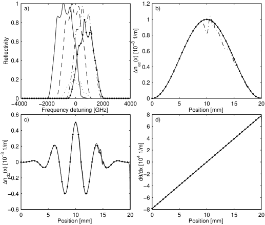
The reflection matrix is applied as input to the layer-stripping method. As the modal indices are similar in magnitude, we use the discrete algorithm directly, and $\boldsymbol{\Upsilon}_{j}$ is calculated by taking into account the factor $(n_{p}+n_{q})/(2n_{0})$ as discussed in Section 3. Moreover, $\boldsymbol{\kappa}(x)$ and $\boldsymbol{\sigma}(x)$ is calculated by inverting the expressions for $\boldsymbol{\rho}_{j}$ and $\boldsymbol{\Phi}_{j}$ in (6d) and (6e), respectively. Figure 2b) shows $\Delta n_{\text{ac}}(x)$ along with its reconstructed version. The reconstructed $\Delta n_{\text{ac}}(x)$ is calculated by a least square fit to (31a) using the diagonal elements of the reconstructed $\boldsymbol{\kappa}(x)$. We find that the error in reconstructed profile is less that $4\cdot 10^{-6}~{}\text{m}^{-1}$. Also shown is the ac modulation profile calculated using scalar layer-stripping on $R_{11}$. Due to the strong coupling between mode 1 and 4, the scalar layer-stripping method does not reconstruct the profile accurately. Figure 2c) and 2d) show that it is possible to separate the dc index variations $\Delta n_{\text{dc}}(x)$ from the grating phase gradient $\text{d}\theta(x)/\text{d}x$. The separation is based on a least square fit to (31b) using the diagonal elements of $\boldsymbol{\sigma}(x)$. The error in reconstructed $\Delta n_{\text{dc}}(x)$ is less than $6\cdot 10^{-5}~{}\text{m}^{-1}$, while the error in reconstructed $\text{d}\theta(x)/\text{d}x$ is less than $300~{}\text{m}^{-1}$. Errors are mainly due to the finite $\Delta x$ in addition to the fact that the reflection matrix spectrum of the discretized structure is strictly nonperiodic (see last paragraph of Section 3).

6 Analogies to 3D inverse scattering

An important inverse scattering problem is the three-dimensional problem associated with the Schrödinger equation [25],

$$\left\{\nabla^{2}+k^{2}-V(x,y,z)\right\}\psi(x,y,z;k)=0,$$ (35)

where $\psi(x,y,z,k)$ is the wave function and $V(x,y,z)$ is a smooth and nonnegative potential with compact support. In particular, solutions to this problem is applicable to inverse seismic scattering. This problem has been solved using a generalized Marchenko method in [25] and [32], while layer-stripping solutions are suggested in [45] and [43]. Note the close resemblance between (35) and (25), indicating that a similar method as that in Section 4 can be used.

We express the solution as a superposition of the eigenmodes of the Schrödinger equation with $V(x,y,z)=0$. Writing $\psi(x,y,z;k)=\Psi(y,z;k_{y},k_{z})\exp(ik_{x}x)$, these eigenmodes are given by

$$\Psi(y,z;k_{y},k_{z})=\exp(i(k_{y}y+k_{z}z)),$$ (36)

where $k_{y}$ and $k_{z}$ are the wave numbers in $y$-direction and $z$-direction, respectively, and $k^{2}=k_{x}^{2}+k_{y}^{2}+k_{z}^{2}$.

In a discrete model, the wavenumbers $k_{y}$ and $k_{z}$ can for example be discretized in equal intervals $\Delta k$, such that $k_{y}=p\Delta k$ and $k_{z}=q\Delta k$. In the $yz$-plane, this means that only a principal range $(-\pi/\Delta k,\pi/\Delta k)$ is considered, and the fields are extended periodically outside this range. The integers $p$ and $q$ are the modal indices satisfying $p^{2}+q^{2}\leq(k/\Delta k)^{2}$ for propagating (not evanescent) modes. The modal field profiles are written in normalized form $\Psi_{pq}(y,z)=(\Delta k/2\pi)\Psi(y,z;p\Delta k,q\Delta k)$. The total field $\psi(x,y,z;k)$ is expressed as the superposition

$$\psi(x,y,z;k)=\sum_{p,q}(b^{+}_{pq}(x)+b^{-}_{pq}(x))\Psi_{pq}(y,z),$$ (37)

where $b^{\pm}_{pq}(x)$ includes all $x$-dependence of the fields, and $\pm$ indicate the sign of $k_{x}$, i.e, the propagation direction of the mode.

As in Section 4, we insert (37) into (35), multiply by $\Psi^{*}_{pq}(y,z)$ and integrate over the principal range of the $yz$-plane. This leads to the coupled mode equations

$$\frac{\text{d}b^{+}_{pq}(x)}{\text{d}x}-ik_{x,pq}b^{+}_{pq}(x) =i\sum_{r,s}\mathcal{C}_{pq,rs}(x)(b^{+}_{rs}(x)+b^{-}_{rs}(x)),$$ (38a)

$$\frac{\text{d}b^{-}_{pq}(x)}{\text{d}x}+ik_{x,pq}b^{-}_{pq}(x) =-i\sum_{r,s}\mathcal{C}_{pq,rs}(x)(b^{+}_{rs}(x)+b^{-}_{rs}(x)),$$ (38b)

where the coupling coefficients are given by

$$\begin{split}\mathcal{C}_{pq,rs}(x)&=-\frac{1}{2k_{x}}\int\Psi^{*}_{pq}(y,z)V(x,y,z)\Psi_{rs}(y,z)\text{d}y\text{d}z\\ &=-\frac{1}{2k_{x}}\left(\frac{\Delta k}{2\pi}\right)^{2}\int V(x,y,z)\exp\left[i\Delta k((r-p)y+(s-q)z)\right]\text{d}y\text{d}z,\end{split}$$ (39)

and $k_{x,pq}=[k^{2}-(\Delta k)^{2}(p^{2}+q^{2})]^{1/2}$. We restrict ourselves to the situation where $V(x,y,z)$ is known to be quasi-periodic along the $x$-direction. Then an expansion of $\mathcal{C}_{pq,rs}(x)$ as in (28) together with the transformation (29) can be used, resulting in the exact same problem as that described in Section 4. Thus the layer-stripping method in Section 3 can be applied. The required input data is the reflection into all plane waves upon excitation of the different plane waves onto the plane $x=0$. The scattering potential $V(x,y,z)$ is found from the inverse of (39).

There are two complications. First, in order to use the factorization methods developed in Section 3, we must ensure that reciprocity implies symmetric scattering matrices. This is guaranteed when the mode profiles can be written real. Thus we define real mode fields by the transformation

$$\begin{bmatrix}{\boldsymbol{\Psi}}_{++}\\ {\boldsymbol{\Psi}}_{-+}\\ {\boldsymbol{\Psi}}_{+-}\\ {\boldsymbol{\Psi}}_{--}\end{bmatrix}\to\mathbf{M}\begin{bmatrix}{\boldsymbol{\Psi}}_{++}\\ {\boldsymbol{\Psi}}_{-+}\\ {\boldsymbol{\Psi}}_{+-}\\ {\boldsymbol{\Psi}}_{--}\end{bmatrix},\quad\mathbf{M}=\frac{1}{2}\begin{bmatrix}\boldsymbol{I}&\boldsymbol{I}&\boldsymbol{I}&\boldsymbol{I}\\ -i\boldsymbol{I}&+i\boldsymbol{I}&-i\boldsymbol{I}&+i\boldsymbol{I}\\ i\boldsymbol{I}&-i\boldsymbol{I}&+i\boldsymbol{I}&+i\boldsymbol{I}-\\ \boldsymbol{I}&\boldsymbol{I}&\boldsymbol{I}&-\boldsymbol{I}\end{bmatrix}.$$ (40)

Here, ${\boldsymbol{\Psi}}_{++}$ denotes a column vector containing the modal field amplitudes $\Psi_{pq}$ with positive $p$ and $q$; ${\boldsymbol{\Psi}}_{-+}$ denotes a column vector containing the modal field amplitudes with negative $p$ and positive $q$, and so forth. The dimension of the identity matrices in the blocks of $\mathbf{M}$ corresponds to the dimension of ${\boldsymbol{\Psi}}_{++}$. If $\mathbf{\mathcal{C}}$ denotes the matrix formed by the elements $\mathcal{C}_{pq,rs}$, the coupling matrix transforms $\mathbf{\mathcal{C}}\to\mathbf{M}^{*}\mathbf{\mathcal{C}}\mathbf{M}^{\text{T}}$. Inspection of (39) shows that the transformed $-\mathbf{\mathcal{C}}$ is real and positive semidefinite (recall that $V(x,y,z)\geq 0$); thus enabling the factorization method in Section 3.

Second, the causality argument of the layer-stripping method does only work when the coupling matrix $\mathbf{\mathcal{C}}$ is independent on frequency. Eq. (39) shows that this condition can only be justified when the relevant frequency band is narrow. Therefore the structure must, in addition to be quasi-periodic along the $x$-direction, vary slowly along the transversal direction. The variation must be sufficiently slow such that the modes with $(p^{2}+q^{2})\Delta k^{2}\ll k^{2}$ contain sufficient information about the transversal dependence, and the other modes may be neglected.

7 Conclusion

A layer-stripping method for the inverse scattering of multi-mode structures has been proposed. Ambiguities related to factorization of each layer’s response into codirectional and contradirectional coupling have been discussed. When there are no codirectional coupling, the ambiguities disappear. Also, when the structure to be reconstructed is smooth, there are important cases with simultaneous co- and contradirectional coupling that can be reconstructed uniquely, provided the reflector eigenvalues are nonzero and nondegenerate. Applications to quasi-periodical structures, and analogies to multidimensional inverse scattering have been discussed.

Appendix A Matrix factorizations

A.1 Takagi factorization of complex symmetric matrices

Any complex symmtric matrix $\boldsymbol{\Upsilon}$ can be written

$$\boldsymbol{\Upsilon}=\boldsymbol{U}^{\text{T}}\boldsymbol{\Sigma}\boldsymbol{U},$$ (41)

where $\boldsymbol{U}$ is unitary and $\boldsymbol{\Sigma}$ is diagonal and nonnegative (See e.g. [18], Chapter 4.4). Eq. (41) is called Takagi factorization.

A constructive proof, suitable for implementation, can be given as follows: Singular value decomposition yields

$$\boldsymbol{\Upsilon}=\boldsymbol{V}_{1}\boldsymbol{\Sigma}\boldsymbol{V}_{2},$$ (42)

where $\boldsymbol{V}_{1,2}$ are unitary, and $\boldsymbol{\Sigma}$ is diagonal and nonnegative. Using $\boldsymbol{\Upsilon}=\boldsymbol{\Upsilon}^{\text{T}}$ and $(\boldsymbol{\Upsilon}\boldsymbol{\Upsilon}^{\dagger})^{\text{T}}=\boldsymbol{\Upsilon}^{\dagger}\boldsymbol{\Upsilon}$ we find that $\boldsymbol{W}\boldsymbol{\Sigma}=\boldsymbol{\Sigma}\boldsymbol{W}^{\text{T}}=\boldsymbol{\Sigma}\boldsymbol{W}$, where $\boldsymbol{W}\equiv\boldsymbol{V}_{2}^{*}\boldsymbol{V}_{1}$. Thus, provided $\boldsymbol{\Upsilon}$ is nonsingular, $\boldsymbol{W}$ is symmetric. Then $\sqrt{\boldsymbol{W}}$ can be chosen such that it commutes with $\boldsymbol{\Sigma}$ and is symmetric, and we obtain $\boldsymbol{\Upsilon}=\boldsymbol{V}_{2}^{\text{T}}\boldsymbol{W}\boldsymbol{\Sigma}\boldsymbol{V}_{2}=(\sqrt{\boldsymbol{W}}\boldsymbol{V}_{2})^{\text{T}}\boldsymbol{\Sigma}\sqrt{\boldsymbol{W}}\boldsymbol{V}_{2}$, or

$$\boldsymbol{\Upsilon}=\boldsymbol{U}^{\text{T}}\boldsymbol{\Sigma}\boldsymbol{U},$$ (43)

where $\boldsymbol{U}\equiv\sqrt{\boldsymbol{W}}\boldsymbol{V}_{2}$ is unitary and $\boldsymbol{\Sigma}$ is diagonal and positive.

If $\boldsymbol{\Upsilon}$ is singular, we write

$$\boldsymbol{\Sigma}=\begin{bmatrix}\boldsymbol{\Sigma}^{\prime}&\boldsymbol{0}\\ \boldsymbol{0}&\boldsymbol{0}\end{bmatrix}\qquad\text{and}\qquad\boldsymbol{W}=\begin{bmatrix}\boldsymbol{W}_{11}&\boldsymbol{W}_{12}\\ \boldsymbol{W}_{21}&\boldsymbol{W}_{22}\end{bmatrix},$$ (44)

where we have arranged $\boldsymbol{\Sigma}$ so that the zero singular values are the last ones, $\boldsymbol{\Sigma}^{\prime}$ is a diagonal matrix with the nonzero singular values, and $\boldsymbol{W}_{11}$ has the same dimension as $\boldsymbol{\Sigma}^{\prime}$. We now find $\boldsymbol{\Sigma}^{\prime}\boldsymbol{W}_{11}=\boldsymbol{W}_{11}\boldsymbol{\Sigma}^{\prime}$, $\boldsymbol{W}_{12}=\boldsymbol{W}_{21}=\boldsymbol{0}$, and $\boldsymbol{W}_{11}=\boldsymbol{W}_{11}^{\text{T}}$. The commutation relations do not provide any information on $\boldsymbol{W}_{22}$. Choose $\sqrt{\boldsymbol{W}}$ such that

$$\sqrt{\boldsymbol{W}}=\begin{bmatrix}\sqrt{\boldsymbol{W}_{11}}&\boldsymbol{0}\\ \boldsymbol{0}&\sqrt{\boldsymbol{W}_{22}}\end{bmatrix},$$ (45)

where $\sqrt{\boldsymbol{W}_{11}}$ is symmetric and $\sqrt{\boldsymbol{W}_{11}}$ and $\boldsymbol{\Sigma}^{\prime}$ commute. Write $\boldsymbol{\Upsilon}=\boldsymbol{U}_{1}^{\text{T}}\boldsymbol{\Sigma}\boldsymbol{U}_{2}$, with

$$\boldsymbol{U}_{1} =\sqrt{\boldsymbol{W}}^{\text{T}}\boldsymbol{V}_{2}=\begin{bmatrix}\boldsymbol{U}^{\prime}\\ \boldsymbol{U}^{\prime\prime}_{1}\end{bmatrix}$$ (46)

$$\boldsymbol{U}_{2} =\sqrt{\boldsymbol{W}}\boldsymbol{V}_{2}=\begin{bmatrix}\boldsymbol{U}^{\prime}\\ \boldsymbol{U}^{\prime\prime}_{2}\end{bmatrix}.$$ (47)

The matrices $\boldsymbol{U}^{\prime\prime}_{1}$ and $\boldsymbol{U}^{\prime\prime}_{2}$ are the rows of $\boldsymbol{U}_{1}$ and $\boldsymbol{U}_{2}$ that correspond to the zero singular values, and they do not give any contribution to $\boldsymbol{\Upsilon}$. We may therefore replace the rows $\boldsymbol{U}^{\prime\prime}_{1}$ by $\boldsymbol{U}^{\prime\prime}_{2}$, which gives $\boldsymbol{U}_{1}=\boldsymbol{U}_{2}=\boldsymbol{U}$.

The matrix $\boldsymbol{\Sigma}$ is unique up to reordering of the singular values. When the order of the singular values is established, $\boldsymbol{U}$ is unique up to the replacement $\boldsymbol{J}\boldsymbol{U}\to\boldsymbol{U}$, where $\boldsymbol{J}$ is a unitary matrix satisfying $(\boldsymbol{J}\boldsymbol{U})^{\text{T}}\boldsymbol{\Sigma}\boldsymbol{J}\boldsymbol{U}=\boldsymbol{U}^{\text{T}}\boldsymbol{\Sigma}\boldsymbol{U}$. This leads to $\boldsymbol{J}^{\text{T}}\boldsymbol{\Sigma}\boldsymbol{J}=\boldsymbol{\Sigma}$. Assuming the singular values are sorted in, say, descending order, we find that $\boldsymbol{J}$ is a unitary block-diagonal matrix, where each block has a dimension equal to the number of corresponding repeated singular values. For zero singular values, the corresponding block in $\boldsymbol{J}$ is an arbitrary unitary matrix. For repeated non-zero singular values, the corresponding block in $\boldsymbol{J}$ is real. For a distinct, non-zero singular value, the corresponding block of $\boldsymbol{J}$ is either 1 or $-1$.

A.2 Factorization of a unitary matrix into a symmetric matrix and an orthogonal matrix

A unitary matrix $\boldsymbol{U}$ can be factorized into $\boldsymbol{U}=\boldsymbol{P}\boldsymbol{\Phi}$, where $\boldsymbol{P}$ is a real unitary matrix (orthogonal matrix) and $\boldsymbol{\Phi}$ is a symmetric unitary matrix (See e.g. [18], Chapter 3.4). A constructive proof, suitable for implementation, can be given as follows. First we note that the symmetric unitary matrix $\boldsymbol{\Phi}$ can be factorized into $\boldsymbol{\Phi}=\boldsymbol{P}_{1}\boldsymbol{D}\boldsymbol{P}_{1}^{\text{T}}$, where $\boldsymbol{D}$ is a diagonal unitary matrix and $\boldsymbol{P}_{1}$ is a real unitary matrix (a simple, constructive proof for this particular spectral decomposition is given in [18], Chapter 4.4). Thus, an equivalent problem is to show that

$$\boldsymbol{U}=\boldsymbol{P}_{2}\boldsymbol{D}\boldsymbol{P}_{1}^{\text{T}},$$ (48)

where $\boldsymbol{P}_{2}=\boldsymbol{P}\boldsymbol{P}_{1}$. The decomposition in (48) is very similar to singular value decomposition of real matrices, except that $\boldsymbol{D}$ may have complex elements.

The matrix $\boldsymbol{U}^{\text{T}}\boldsymbol{U}$ is unitary and symmetric; thus we can write

$$\boldsymbol{U}^{\text{T}}\boldsymbol{U}=\boldsymbol{P}_{1}\boldsymbol{\Lambda}\boldsymbol{P}_{1}^{\text{T}},$$ (49)

where $\boldsymbol{P}_{1}$ is a real unitary matrix and $\boldsymbol{\Lambda}$ is a diagonal unitary matrix. Define

$$\boldsymbol{P}_{2}=\boldsymbol{U}\boldsymbol{P}_{1}\boldsymbol{D}^{*},$$ (50)

where the diagonal matrix $\boldsymbol{D}$ is a solution to $\boldsymbol{D}^{2}=\boldsymbol{\Lambda}$. The matrix $\boldsymbol{P}_{2}$ is unitary since it is produced by multiplication of unitary matrices, thus $\boldsymbol{P}_{2}^{*}\boldsymbol{P}_{2}^{\text{T}}=\boldsymbol{I}$. The matrix is also real since

$$\boldsymbol{P}_{2}^{\text{T}}\boldsymbol{P}_{2}=\boldsymbol{D}^{*}\boldsymbol{P}_{1}^{\text{T}}\boldsymbol{U}^{\text{T}}\boldsymbol{U}\boldsymbol{P}_{1}\boldsymbol{D}^{*}=\boldsymbol{D}^{*}\boldsymbol{P}_{1}^{\text{T}}\boldsymbol{P}_{1}\boldsymbol{D}^{2}\boldsymbol{P}_{1}^{\text{T}}\boldsymbol{P}_{1}\boldsymbol{D}^{*}=\boldsymbol{I},$$ (51)

which gives $\boldsymbol{P}_{2}=(\boldsymbol{P}_{2}^{*}\boldsymbol{P}_{2}^{\text{T}})\boldsymbol{P}_{2}=\boldsymbol{P}_{2}^{*}(\boldsymbol{P}_{2}^{\text{T}}\boldsymbol{P}_{2})=\boldsymbol{P}_{2}^{*}$.

From (50) we therefore conclude that the decomposition (48), with real unitary $\boldsymbol{P}_{1}$ and $\boldsymbol{P}_{2}$ and diagonal $\boldsymbol{D}$, is always possible. It follows that any unitary matrix can be written $\boldsymbol{U}=\boldsymbol{P}\boldsymbol{\Phi}$, where $\boldsymbol{P}$ is real and unitary, and $\boldsymbol{\Phi}$ is symmetric and unitary. Note that any global phase of $\boldsymbol{P}$ can instead be assigned to $\boldsymbol{\Phi}$, so without loss of generality we can assume that $\boldsymbol{P}$ is special ($\det\boldsymbol{P}=1$ and $\det\boldsymbol{\Phi}=\det\boldsymbol{U}$).

Since $\boldsymbol{D}$ is calculated from $\boldsymbol{D}^{2}=\boldsymbol{\Lambda}$, the sign of its elements are arbitrary. The ambiguities when determining $\boldsymbol{P}_{1}$ in (49) give rise to ambiguities in $\boldsymbol{P}$ and $\boldsymbol{\Phi}$. The possible $\boldsymbol{P}$ and $\boldsymbol{\Phi}$ can be expressed as $\boldsymbol{P}=\boldsymbol{U}\boldsymbol{P}_{1}\boldsymbol{J}\boldsymbol{D}^{*}\boldsymbol{J}^{\text{T}}\boldsymbol{P}_{1}^{\text{T}}$ and $\boldsymbol{\Phi}=\boldsymbol{P}_{1}\boldsymbol{J}\boldsymbol{D}\boldsymbol{J}^{T}\boldsymbol{P}_{1}^{\text{T}}$ for a real unitary $\boldsymbol{J}$ that commutes with $\boldsymbol{D}^{2}$. Here $\boldsymbol{P}_{1}$ is fixed. If the signs of the elements of $\boldsymbol{D}$ are known to be such that any equal elements of $\boldsymbol{D}^{2}$ correspond to equal elements of $\boldsymbol{D}$, then $\boldsymbol{J}$ commutes with $\boldsymbol{D}$ and can be ignored.

Appendix B Linear, reciprocal and lossless components

Consider a linear component with $P$ input and $P$ output modes on the left-hand side, and also $P$ input and $P$ output modes on the right-hand side, see Fig. 3.

Fig. 3: A linear component with $P$ input and $P$ output modes on each side.

The component is completely characterized by the $2P\times 2P$ dimensional scattering matrix $\mathbf{S}$ which relates the input and output fields:

$$\begin{bmatrix}\boldsymbol{v}_{1}\\ \boldsymbol{u}_{2}\end{bmatrix}=\mathbf{S}\begin{bmatrix}\boldsymbol{u}_{1}\\ \boldsymbol{v}_{2}\end{bmatrix}=\begin{bmatrix}\boldsymbol{S}_{11}&\boldsymbol{S}_{12}\\ \boldsymbol{S}_{21}&\boldsymbol{S}_{22}\end{bmatrix}\begin{bmatrix}\boldsymbol{u}_{1}\\ \boldsymbol{v}_{2}\end{bmatrix}.$$ (52)

The field vectors that propagate to the right and left are denoted $\boldsymbol{u}$ and $\boldsymbol{v}$, respectively, and the subscripts 1 and 2 indicate the left- and right-hand side of the component. The scattering matrix is a block matrix; the blocks $\boldsymbol{S}_{11}$ and $\boldsymbol{S}_{22}$ being the reflection from the left and right side of the device, respectively, and $\boldsymbol{S}_{21}$ and $\boldsymbol{S}_{12}$ the transmission through the device from the left and right, respectively. These blocks have the dimension $P\times P$.

There exists a similar relation, a transfer matrix relation, that connects the fields on the left-hand side to the fields on the right-hand side:

$$\begin{bmatrix}\boldsymbol{u}_{2}\\ \boldsymbol{v}_{2}\end{bmatrix}=\mathbf{T}\begin{bmatrix}\boldsymbol{u}_{1}\\ \boldsymbol{v}_{1}\end{bmatrix}.$$ (53)

Comparing (52) and (53) we find the blocks of $\mathbf{T}$:

$$\mathbf{T}=\begin{bmatrix}\boldsymbol{S}_{21}-\boldsymbol{S}_{22}\boldsymbol{S}_{12}^{-1}\boldsymbol{S}_{11}&\boldsymbol{S}_{22}\boldsymbol{S}_{12}^{-1}\\ -\boldsymbol{S}_{12}^{-1}\boldsymbol{S}_{11}&\boldsymbol{S}_{12}^{-1}\end{bmatrix}.$$ (54)

To describe a device with a transfer matrix, $\boldsymbol{S}_{12}$ must be invertible, that is the transmission from the right cannot be zero for any input field vector. Thus, ideal mirrors, for example, cannot be described by a transfer matrix.

Provided the mode profiles can be written real, reciprocity means that the scattering matrix is symmetric [29, 15], i.e.,

$$\boldsymbol{S}_{11} =\boldsymbol{S}_{11}^{\text{T}}$$ (55a)

$$\boldsymbol{S}_{22} =\boldsymbol{S}_{22}^{\text{T}}$$ (55b)

$$\boldsymbol{S}_{21} =\boldsymbol{S}_{12}^{\text{T}}.$$ (55c)

Moreover, the lossless condition is expressed as the unitarity condition $\mathbf{S}^{\dagger}\mathbf{S}=\mathbf{I}$:

$$\boldsymbol{S}_{11}^{\dagger}\boldsymbol{S}_{11}+\boldsymbol{S}_{21}^{\dagger}\boldsymbol{S}_{21} =\boldsymbol{I}$$ (56a)

$$\boldsymbol{S}_{12}^{\dagger}\boldsymbol{S}_{12}+\boldsymbol{S}_{22}^{\dagger}\boldsymbol{S}_{22} =\boldsymbol{I}$$ (56b)

$$\boldsymbol{S}_{12}^{\dagger}\boldsymbol{S}_{11}+\boldsymbol{S}_{22}^{\dagger}\boldsymbol{S}_{21} =\boldsymbol{0}.$$ (56c)

With (55) in mind, we introduce Takagi factorization of $\boldsymbol{S}_{11}$ and $-\boldsymbol{S}_{22}$ (see Appendix A.1):

$$\boldsymbol{S}_{11} =\boldsymbol{\Phi}_{\text{l}}^{\text{T}}\boldsymbol{\rho}\boldsymbol{\Phi}_{\text{l}}$$ (57a)

$$\boldsymbol{S}_{22} =\boldsymbol{\Phi}_{\text{r}}(-\boldsymbol{\rho}^{\prime})\boldsymbol{\Phi}_{\text{r}}^{\text{T}}$$ (57b)

$$\boldsymbol{S}_{21} =\boldsymbol{\Phi}_{\text{r}}\boldsymbol{t}^{\prime}\boldsymbol{\Phi}_{\text{l}}.$$ (57c)

Here, $\boldsymbol{\Phi}_{\text{l}}$ and $\boldsymbol{\Phi}_{\text{r}}$ are unitary matrices, $\boldsymbol{\rho}$ and $\boldsymbol{\rho}^{\prime}$ are diagonal and nonnegative, and $\boldsymbol{t}^{\prime}=\boldsymbol{\Phi}_{\text{r}}^{\dagger}\boldsymbol{S}_{21}\boldsymbol{\Phi}_{\text{l}}^{\dagger}$. By substituting into (56) and using (55) we obtain

$$\boldsymbol{t}^{\prime\dagger}\boldsymbol{t}^{\prime}=\boldsymbol{I}-\boldsymbol{\rho}^{2}$$ (58a)

$$\boldsymbol{t}^{\prime}\boldsymbol{t}^{\prime\dagger}=\boldsymbol{I}-\boldsymbol{\rho}^{\prime 2}$$ (58b)

$$\boldsymbol{\rho}^{\prime}=\boldsymbol{t}^{\prime}\boldsymbol{\rho}\boldsymbol{t}^{\prime*-1}.$$ (58c)

Introducing the singular value decomposition $\boldsymbol{t}^{\prime}=\boldsymbol{U}^{\prime}\boldsymbol{t}\boldsymbol{V}^{\prime}$, we obtain from (58a) that $\boldsymbol{t}^{2}=\boldsymbol{V}^{\prime}(\boldsymbol{I}-\boldsymbol{\rho}^{2})\boldsymbol{V}^{\prime\dagger}$, which means $\boldsymbol{t}=\boldsymbol{V}^{\prime}\sqrt{\boldsymbol{I}-\boldsymbol{\rho}^{2}}\boldsymbol{V}^{\prime\dagger}$. Backsubstitution shows that $\boldsymbol{t}^{\prime}$ can be written $\boldsymbol{t}^{\prime}=\boldsymbol{U}\sqrt{\boldsymbol{I}-\boldsymbol{\rho}^{2}}$ for a unitary $\boldsymbol{U}$; thus (58c) reduces to $\boldsymbol{\rho}^{\prime}=\boldsymbol{U}\boldsymbol{\rho}\boldsymbol{U}^{\text{T}}$. With these properties, it is straightforward to show that (57) can be written

$$\boldsymbol{S}_{11} =\boldsymbol{\Phi}_{\text{l}}^{\text{T}}\boldsymbol{\rho}\boldsymbol{\Phi}_{\text{l}}$$ (59a)

$$\boldsymbol{S}_{22} =\boldsymbol{\Phi}_{\text{r}}(-\boldsymbol{\rho})\boldsymbol{\Phi}_{\text{r}}^{\text{T}}$$ (59b)

$$\boldsymbol{S}_{21} =\boldsymbol{S}_{12}^{\text{T}}=\boldsymbol{\Phi}_{\text{r}}\boldsymbol{t}\boldsymbol{\Phi}_{\text{l}},$$ (59c)

where $\boldsymbol{U}$ has been absorbed into $\boldsymbol{\Phi}_{\text{r}}$, $\boldsymbol{\Phi}_{\text{r}}\boldsymbol{U}\rightarrow\boldsymbol{\Phi}_{\text{r}}$, and

$$\boldsymbol{t}=\sqrt{\boldsymbol{I}-\boldsymbol{\rho}^{2}}.$$ (60)

Note that (58) implies that $\|\boldsymbol{\rho}\|\leq 1$.

Eq. (59) and (60) can be interpreted as follows: The component can be viewed as a discrete reflector sandwiched between two unitary transmission sections. The discrete reflector provides coupling between equal modes that propagate in opposite directions, and the unitary sections provide coupling between different modes in the same direction. For the discrete reflector, the reflection response from the left and right is $\boldsymbol{\rho}$ and $-\boldsymbol{\rho}$, respectively, and the transmission is $\boldsymbol{t}$. For the two unitary sections, there are no reflections, and the transmission responses from the left are $\boldsymbol{\Phi}_{\text{l}}$ and $\boldsymbol{\Phi}_{\text{r}}$, while the transmission responses from the right are $\boldsymbol{\Phi}_{\text{l}}^{\text{T}}$ and $\boldsymbol{\Phi}_{\text{r}}^{\text{T}}$. Note that this interpretation is consistent with the reciprocity and lossless conditions (55) and (56), for each of the three sections separately. By inspection, we find that (59) is invariant if $\boldsymbol{P}\boldsymbol{\rho}\boldsymbol{P}^{\text{T}}\rightarrow\boldsymbol{\rho}$, $\boldsymbol{P}\boldsymbol{t}\boldsymbol{P}^{\text{T}}\rightarrow\boldsymbol{t}$, $\boldsymbol{P}\boldsymbol{\Phi}_{\text{l}}\rightarrow\boldsymbol{\Phi}_{\text{l}}$, and $\boldsymbol{\Phi}_{\text{r}}\boldsymbol{P}^{\text{T}}\rightarrow\boldsymbol{\Phi}_{\text{r}}$ where $\boldsymbol{P}$ is a real unitary matrix. Here $\boldsymbol{P}$ represents an arbitrary rotation of the eigenaxes of the reflector ($\boldsymbol{\rho}$ and $\boldsymbol{t}$ are now real and positive semidefinite).

Using (59), the transfer matrix (54) can be written

$$\mathbf{T}=\begin{bmatrix}\boldsymbol{A}^{*}&\boldsymbol{B}^{*}\\ \boldsymbol{B}&\boldsymbol{A}\end{bmatrix},$$ (61)

where the blocks $\boldsymbol{A}=\boldsymbol{\Phi}_{r}^{*}\boldsymbol{t}^{-1}\boldsymbol{\Phi}_{l}^{*}$ and $\boldsymbol{B}=-\boldsymbol{\Phi}_{r}^{*}\boldsymbol{t}^{-1}\boldsymbol{\rho}\boldsymbol{\Phi}_{l}$ satisfy

$$\boldsymbol{A}^{\dagger}\boldsymbol{A}-\boldsymbol{B}^{\text{T}}\boldsymbol{B}^{*} =\boldsymbol{I}$$ (62a)

$$\boldsymbol{A}\boldsymbol{B}^{\text{T}}-\boldsymbol{B}\boldsymbol{A}^{\text{T}} =\boldsymbol{0}$$ (62b)

$$\boldsymbol{A}^{\text{T}}\boldsymbol{B}^{*}-\boldsymbol{B}^{\dagger}\boldsymbol{A} =\boldsymbol{0}.$$ (62c)

References

- [1] T. Aktosun, M. Klaus, and C van der Mee, Direct and inverse scattering for selfadjoint Hamiltonian systems on the line, Integr. Equ. Oper. Theory, 38 (2000), pp. 129–171.
- [2] V. Bardan, Comments on dynamic predictive deconvolution, Geophys. Prosp., 25 (1977), pp. 569–572.
- [3] A. Boutet de Monvel and V. Marchenko, New inverse spectral problem and its application, in Inverse and algebraic quantum scattering theory (Lake Balaton, 1996), vol. 488 of Lecture Notes in Phys., Springer, Berlin, 1997, pp. 1–12.
- [4] J. K. Brenne and J. Skaar, Design of grating-assisted codirectional couplers with discrete inverse-scattering algorithms, J. Lightwave Technol., 21 (2003), pp. 254–263.
- [5] A. M. Bruckstein and T. Kailath, Inverse scattering for discrete transmission-line models, SIAM Rev., 29 (1987), pp. 359–389.
- [6] A. M. Bruckstein, B. C. Levy, and T. Kailath, Differential methods in inverse scattering, SIAM J. Appl. Math., 45 (1985), pp. 312–335.
- [7] L. Dong, L. Reekie, J. L. Cruz, J. E. Caplen, J. P. deSandro, and D. N. Payne, Optical fibers with depressed claddings for suppression of coupling into cladding modes in fiber Bragg gratings, IEEE Photonics Technology Letters, 9 (1997), pp. 64–66.
- [8] T. Erdogan, Cladding-mode resonances in short- and long-period fiber grating filters, Journal Of The Optical Society Of America A-Optics Image Science And Vision, 14 (1997), pp. 1760–1773.
- [9] R. Feced and M. N. Zervas, Efficient inverse scattering algorithm for the design of grating-assisted codirectional mode couplers, J. Opt. Soc. Am. A, 17 (2000), pp. 1573–1582.
- [10] R. Feced, M. N. Zervas, and M. A. Muriel, An efficient inverse scattering algorithm for the design of nonuniform fiber Bragg gratings, IEEE J. Quantum Electron., 35 (1999), pp. 1105–1115.
- [11] V. Finazzi and M. Zervas, Cladding mode losses in chirped Bragg gratings, in Bragg Gratings, Photosensitivity, and Poling in glass waveguides (BGPP), OSA Technical Digest, Washington, D.C., 2001, Optical Society of America, p. BMG16.
- [12] M. Foggatt, Distributed measurement of the complex modulation of a photoinduced bragg grating in an optical fiber, Applied Optics, 35 (1996), pp. 5162–5164.
- [13] I. M. Gel’fand and B. M. Levitan, On the determination of a differential equation from its spectral function, Amer. Math. Soc. Transl. (2), 1 (1955), pp. 253–304.
- [14] F. Ghiringhelli and M. Zervas, Inverse scattering design of fiber Bragg gratings with cladding mode losses compensation, in Bragg Gratings, Photosensitivity, and Poling in glass waveguides (BGPP), vol. 94 of OSA Topic in Optics and Photonics Series, Washington, D.C., 2003, Optical Society of America, p. TuD2.
- [15] H. A. Haus, Electromagnetic noise and quantum optical measurements, Springer, 2000.
- [16] K. O. Hill, F. Bilodeau, B. Malo, and D. C. Johnson, Birefringent photosensitivity in monomode optical fibre: application to external writing of rocking filters, J. Opt. Soc. Am. B, 27 (1991), pp. 1548–1550.
- [17] K. O. Hill and G. Meltz, Fiber Bragg grating technology: Fundamentals and overview, J. Lightwave Technol., 15 (1997), pp. 1263–1276.
- [18] R. A. Horn and C. A. Johnson, Matrix analysis, Cambridge, 1985.
- [19] K. Jinguji and M. Kawachi, Synthesis of coherent two-port lattice-form optical delay-line circuit, J. Lightwave Tech., 13 (1995), pp. 73–82.
- [20] R. C. Jones, A new calculus for the treatment of optical systems, J. Opt. Soc. Am., 31 (1941), pp. 488–503.
- [21] H. Kogelnik, Theory of Optical Waveguides, Guided-Wave Optoelectronics, New York: Springer-Verlag, 1990.
- [22] M. Kreĭn, On a method of effective solution of an inverse boundary problem, Doklady Akad. Nauk SSSR (N.S.), 94 (1954), pp. 987–990.
- [23] H. P. Li, Y. Nakamura, K. Ogusu, Y. L. Sheng, and J. E. Rothenberg, Influence of cladding-mode coupling losses on the spectrum of a linearly chirped multi-channel fiber Bragg grating, Optics Express, 13 (2005), pp. 1281–1290.
- [24] D. Marcuse, Theory of Dielectric Optical Waveguides, New York: Academic, 1991.
- [25] R.G. Newton, Inverse scattering. II. Three dimensions, Journal of Mathematical Physics, 21 (1980), pp. 1698–1715.
- [26] F. Ouellette, Dispersion cancellation using linearly chirped Bragg grating filters in optical wave-guides, Optics Letters, 12 (1987), pp. 847–849.
- [27] F. Ouellette, P. A. Krug, T. Stephens, G. Dhosi, and B. Eggleton, Broad-band and WDM dispersion compensation using chirped sampled fiber Bragg gratings, Electronics Letters, 31 (1995), pp. 899–901.
- [28] C. L. Pekeris, Direct method of interpretation in resistivity prospecting, Geophysics, 5 (1940), pp. 31–42.
- [29] D. M. Pozar, Microwave engineering, Addison-Wesley, 1993.
- [30] Rakesh, A one-dimensional inverse problem for a hyperbolic system with complex coefficients, Inv. Prob., 17 (2001), pp. 1401–1417.
- [31] E. A. Robinson, Dynamic predictive deconvolution, Geophys. Prosp., 23 (1975), pp. 779–797.
- [32] J.H. Rose, The connection between time- and frequency-domain three-dimensional inverse scattering methods, Journal of Mathematical Physics, 25 (1984), pp. 2995–3000.
- [33] A. Rosenhal, M. Horowitz, S. Lange, and C. Shäffer, Experimental reconstruction of a long-period grating from its core-to-core spectrum, Optics Letters, 30 (2005), pp. 3272–3274.
- [34] A. Rosenthal and M. Horowitz, Inverse scattering algorithm for reconstructing strongly reflecting fiber Bragg gratings, IEEE J. Quantum Electron., 39 (2003), pp. 1018–1026.
- [35] D. Sandel, R. Noé, G. Heise, and B. Borchert, Optical network analysis and longitudinal structure characterization of fiber Bragg grating, J. Lightwave Technol., 16 (1998), pp. 2435–2442.
- [36] J. Skaar and O. H. Waagaard, Design and characterization of finite length fiber gratings, IEEE J. Quantum Electron., 39 (2003), pp. 1238–1245.
- [37] J. Skaar, L. Wang, and T. Erdogan, On the synthesis of fiber Bragg gratings by layer peeling, IEEE J. Quantum Electron., 37 (2001), pp. 165–173.
- [38] A. W. Snyder and J. D. Love, Optical Waveguide Theory, Chapman & Hall, 1983.
- [39] G.-H Song, Toward the ideal codirectional Bragg filter with an acousto-optic-filter design, J. Lightwave Technol., 13 (1995), pp. 470–480.
- [40] G.-H Song and S.-Y Shin, Design of corrugated waveguide filters by the Gel’fand-Levitan-Marchenko inverse-scattering method, J. Opt. Soc. Am. A, 2 (1985), pp. 1905–1915.
- [41] O. H. Waagaard and J. Skaar, Synthesis of birefringent reflective gratings, J. Opt. Soc. Am. A, 21 (2004), pp. 1207–1220.
- [42] L. Wang and T. Erdogan, Layer peeling algorithm for reconstruction of long-period fibre gratings, Electron. Lett., 37 (2001), pp. 154–156.
- [43] A. E. Yagle, Differential and integral methods for multidimensional inverse scattering problems, Journal of Mathematical Physics, 27 (1986), pp. 2584–2591.
- [44] A. E. Yagle and J. L. Frolik, On the feasibility of impulse reflection response data for the two-dimensional inverse scattering problem, IEEE Transactions on Antennas and Propagation, 44 (1996), pp. 1551–1564.
- [45] A. E. Yagle and B. C. Levy, Layer-stripping solutions of multidimensional inverse scattering problems, Journal of Mathematical Physics, 27 (1986), pp. 1701–1710.