Effect of a fluctuating parameter mismatch in coupled Rössler systems

Abstract

This paper is concerned with the effect of parameter fluctuations with a characteristic waiting time in coupled Rössler oscillators. We show that the averaged error in synchronization that is introduced due to a fluctuating parameter is proportional to the waiting time and the amplitude of the fluctuations. It is also shown that coupling strength beyond a threshold value does not have any significant effect on improving the quality of synchronization when the fluctuations posses considerable waiting time.

Synchronization of coupled chaotic systems has generated a lot of research activities over the last several years [1, 2, 3]. Synchronized chaotic behavior has been studied extensively in physical, chemical and biological systems. One of the frequently employed methods is coupling two identical systems, this coupling may be unidirectional or bidirectional. Complete synchronization of identical chaotic systems is of considerable interest because of its applications in secure communication[4, 6, 5, 7]. By identical systems we mean a set of systems whose parameters are exactly equal. It is found that complete synchronization is not possible when there is a small but finite mismatch of the parameters of the systems. In coupled non autonomous systems effect of a phase mismatch or finite constant frequency detuning is to destroy the synchronization altogether[9].

Coupled Rössler oscillators have been extensively used for studies in synchronization. This is due to their simplicity and results obtained can usually be generalized to other chaotic systems. Kurths. et. al have shown that coupled Rössler systems which possess parameter mismatch attain a state of phase synchronization[10] and on increasing the coupling strength, such systems may synchronize, but lagged in time [11]. It is also found that many systems, both mathematical models and actual physical systems, show similar behavior [12]. There remains a question as to what happen if the parameter mismatch is fluctuating. Such a study is relevant and important since in reality it is difficult, if not impossible, to construct identical systems except in numerical simulations. This can also be due to the fact that the parameters could be fluctuating in time with time scales of their own, either due to internal instabilities or due to some external perturbations. In this paper we discuss the effect of fluctuating parameters and the effect of timescales associated with such fluctuations on the synchronization of coupled Rössler oscillators.

1 Parameter fluctuations

Let us consider the parameters $p_{1}$ and $p_{2}$ of a coupled system of oscillators which fluctuates randomly. The fluctuations are assumed to occur in time as follows

$$p_{1t}=p_{0}+\xi_{1t}$$ (1)

$$p_{2t}=p_{0}+\xi_{2t},$$

where, $\xi_{1t}$ and $\xi_{2t}$ are two delta correlated zero mean random variables and $p_{0}$ be some average value of the parameters. It is also assumed that the the fluctuations have a waiting time $\tau_{0}$. That is $\tau_{0}$ is the time for which the parameter retains its value before it is changed once again. We define the fluctuation rate $\phi$, as the number of times a parameter is perturbed in unit time which is also the inverse of the waiting time . In a case where the parameter fluctuates in this fashion, it can be seen the the parameter is correlated in time as

$$\rho(p(t)p(t+\tau))=\left\{\begin{array}[]{cc}1-\frac{\tau}{\tau_{0}}&\mbox{if }\tau<\phi\\ \mbox{0}&\mbox{otherwise}\end{array}\right.$$

Where $\rho(..)$ denotes the normalized auto correlation. The amplitude of the parameter mismatch is denoted as $\widetilde{\Delta p}$, given by

$$\widetilde{\Delta p}=\langle\mid\delta p(t)\mid\rangle_{t},$$ (2)

where, $\delta p_{t}=p_{1t}-p_{2t}$ and $\langle...\rangle_{t}$ denotes time average. We did not consider the root mean square value because the system is sensitive to the magnitude of parameter mismatch, not to its square, at least in general. This model of fluctuation is, not the typical, but we believe that this is the closest approximation that can be applied an actual system. Also, it is interesting to note that our model of fluctuation is complimentary to the dichotomic noise [13] where amplitude of fluctuation is a constant, but the waiting time fluctuates about an average.

There is one question that may arise at this point. The systems under consideration is continuous but the fluctuations are discrete. Why continuous fluctuations, for example, an Ornstein Uhlenbeck kind, which posses time scales and are continuous were not considered. Our answer is, such fluctuations arise as a result of a stochastic evolution. As far as complete synchronization is considered, we do not expect such untethered stochastic evolution of parameters in the parameter space. Instead, a parameter, if deviated from its desired value is expected to fluctuate around an average as complete synchronization is usually not found in nature but found in fabricated systems, well monitored and well designed. There, we expect if a parameter mismatch occurs, it will have a tendency or it will be forced to cross zero very often. In such a situation the prime consideration shall be the time scales associated with the fluctuations.

2 Effect of Fluctuations on Dynamics

In a case where the parameter fluctuating as described in sec. 1 the effect on the dynamics of coupled chaotic system can be understood in terms of the dynamical equations. Let the evolution of the coupled systems in phase space be given by,

$$\dot{X_{1}} = f_{1}(p_{1},X_{1})+Cf(X_{2}-X_{1})$$ (3)

$$\dot{X_{2}} = f_{1}(p_{2},X_{2})+Cf(X_{1}-X_{2}).$$

Where $X$ represents the phase space variables, $p$ the parameter whose fluctuation is considered, and $C$, the coupling strength. With equation (3) we can write an equation for the rate of separation $X_{1}-X_{2}$ of the trajectories as,

$$\frac{d(X_{1}-X_{2})}{dt}=\dot{X_{1}}-\dot{X_{2}}=M(p_{1},p_{2},X_{1},X_{2}),$$ (4)

$M(p_{1},p_{2},X_{1},X_{2})$ is a function of the dynamical variables, the parameters of the coupled systems and $\Delta p$ the parameter mismatch. This can be expanded int terms of $\Delta p$ and the effect of fluctuations can be separated out.

$$M(p_{1},p_{2},X_{1},X_{2}) = M_{s}(p_{0},X_{1},X_{2})$$

$$+E(X_{1},X_{2},\Delta p_{1},\Delta p_{2}).$$

Here $M_{s}(p_{0},X_{1},X_{2})$ represents the quantity which offers a stable synchronization manifold and $E(X_{1},X_{2},\Delta p_{1},\Delta p_{2})$ represents the effect of the parameter mismatch.

Let us now see the form of $E(X_{1},X_{2},\Delta p_{1},\Delta p_{2})$ in the in case of a system of bidirectionally coupled Rössler oscillators.

$$\dot{x}_{1,2} = -y_{1,2}-z_{1,2}+c(x_{2,1}-x_{1,2})$$ (6)

$$\dot{y}_{1,2} = x_{1,2}+p_{1,2}y_{1,2}$$

$$\dot{z}_{1,2} = 0.2+z_{1,2}(x_{1,2}-10)$$

Here it is assumed that in the absence of fluctuations and for an appropriate value of $c$, the systems get synchronized. Also in the presence of fluctuations an approximate synchrony is maintained due to the negative conditional Lyapunov exponents and the zero mean nature of the fluctuations. With equation (6), we can write the rate of separation of trajectories as,

$$\frac{d(x_{1}-x_{2})}{dt} = -y_{1}+y_{2}-z_{1}+z_{2}+2C(x_{2}-x_{1})$$ (7)

$$\frac{d(y_{1}-y_{2})}{dt} = x_{1}-x_{2}+p_{1}y_{1}-p_{2}y_{2}$$

$$\frac{d(z_{1}-z_{2})}{dt} = x_{1}z_{1}-x_{2}z_{2}-10(z_{1}-z_{2}).$$

Here it can be seen that the fluctuations affect the dynamics through $y$, as the parameter $p$ occur only in the equation for $\dot{y}$ in the coupled set of equations. Thus by Taylors expansion around $p_{0}$, $E(X_{1},X_{2},\Delta p_{1},\Delta p_{2})$ can be written as,

$$E(X_{1},X_{2},\Delta p_{1},\Delta p_{2})=y_{1}\xi_{1}-y_{2}\xi_{2}$$ (8)

The evolution of the system in time can be split into several sub intervals of duration $\tau$. Thus in a approximately synchronized state the error occurred due to the fluctuations in the $k^{th}$ interval can be written as,

$$\epsilon(t,t+\tau) = \int_{t}^{t+\tau_{0}}(y_{1}\xi_{1}-y_{2}\xi_{2})dt$$ (9)

If the parameter fluctuation are fast enough $y_{1}$ and $y_{2}$ can be considered to be a constant between two consecutive fluctuations and is denoted by $\overline{y_{1}}$ and $\overline{y_{2}}$. Also $\xi_{1}$ and $\xi_{1}$ are constants for a given waiting time $\tau$ by definition, and their value in the $k^{th}$ interval is $\xi_{1k}$ and $\xi_{2k}$. Thus equation (9) can be written as,

$$\epsilon_{k}(t,t+\tau_{0}) = \int_{t}^{t+\tau}(\overline{y_{1k}}\xi_{1k}-\overline{y_{2k}}\xi_{2k})dt$$

$$= \tau_{0}(\overline{y_{1k}}\xi_{1k}-\overline{y_{2k}}\xi_{2k})$$

From this equation, $\langle\epsilon_{k}^{2}\rangle$ can be calculated

$$\langle\epsilon_{k}^{2}\rangle = \tau_{0}^{2}\langle\overline{y_{1k}}^{2}\xi_{1k}^{2}+\overline{y_{2k}}^{2}\xi_{2k}^{2}\rangle$$ (11)

In the above relation $\langle\overline{y_{1k}}^{2}\xi_{1k}^{2}+\overline{y_{2k}}^{2}\xi_{2k}^{2}\rangle$ can be considered as a constant as $y$ belong to an attractor which is dense in periodic orbits and the averages of $\xi$ over the waiting time follows some well defined statistical distribution. $\langle\epsilon_{k}^{2}\rangle_{t}$ can be written as

$$\langle\epsilon_{k}^{2}\rangle = \tau_{0}^{2}\times constant$$ (12)

as $t~{}\rightarrow~{}\infty$. Here note that this expression do not contain $C$ which is the coupling strength. This suggest that increasing the coupling strength do not have any significant effect on reducing the fluctuations. Also note that the error introduced by fluctuations is proportional to the amplitude of fluctuations.

3 Effect of Fluctuations on the Quality of Synchronization

In the last section we saw that the the fluctuations affect the dynamics in a multiplicative manner and its effect on the seperation of the trajectories is proportional to the waiting time. In this section we consider how the fluctuations affect the over all dynamics of the coupled system. Consider a system where the dynamics is represented by the dynamical equations $\dot{\nu_{i}}~{}=f_{i}(\nu_{1}...\nu_{n})$. The effect of a perturbation of a variable $\nu_{k}$ on the variable $\nu_{j}$ can be written as $\delta\nu_{j}=~{}\frac{\partial f_{j}(\nu_{1}...\nu_{n})}{\partial\nu_{k}}\delta\nu_{k}$. Thus it can be seen that in a situation where the phase space variables can be considered to be a constant, the effect of the perturbation applied to one variable have proportional effect on other variables also.

Effect of such perturbations on the quality of synchronization can be quantified using any measure of synchronization which is based on the divergence of the trajectories of the coupled system. A well known measure of the quality of synchronization which is the similarity function $S(0)$ defined as,

$$S^{2}(0)=\frac{\langle[x_{1}(t)-x_{2}(t)]^{2}\rangle}{[\langle x_{1}^{2}(t)\rangle\langle x_{2}^{2}(t)\rangle]^{\frac{1}{2}}}.$$ (13)

In an ideally synchronized state this directly corresponds to $\epsilon_{k}$. If an approximate synchrony is maintained during the evolution of the system we can assume that the majority of contribution to the error in synchronization is of the form $\epsilon_{k}$. Thus the analysis that we have presented is valid if $S(0)$ can be fitted with a function which is linear in $\tau_{0}$, or proportional to the inverse of $\phi$, the fluctuation rate in an actual numerical experiment.

3.1 Numerical simulations

In figure 1 it can be seen that the coupling strength greater than the threshold value does not play any significant role in determining the quality of synchronization. But the quality increase as the fluctuation rate is increased. In figure 2 curve fitting is done for the coupling strength $c~{}=~{}0.9$, it can be seen that $S(0)$ varies with $\tau_{0}$ as

$$S(0)=a+b\tau_{0}.$$ (14)

where $a=0.005$ and $b=0.12$ In figure 3 it is shown that for two fluctuation rates, $S(0)$ grows linearly with the amplitude of fluctuations, the growth rate of the error is higher for a larger waiting time. Numerically, the results were similar for the averages of $\xi$ over the waiting time following uniform or Gaussian distribution. Thus for a given amplitude of fluctuations it is the time scales associated with the fluctuations that determine the quality of synchronization. Interestingly there are similar results in biological systems [15] with coloured fluctuations that higher correlation times (time scales) makes the coupled systems less synchronizable.

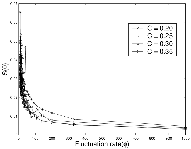
Figure 1: The synchronization error decreases with the increase in the fluctuation rate. It can be seen that high coupling could not stabilize synchronization with lower fluctuation rates. Here $\widetilde{\Delta p}=0.05$.

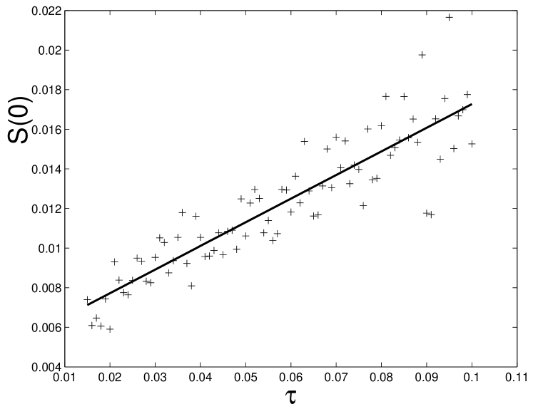
Figure 2: Relation between $\phi$ and $S(0)$ is found to be of the form $S(0)=a+b*\tau_{0}$, a=0.005 and b= 0.12.

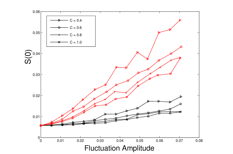
Figure 3: For two fluctuation rates, $\phi~{}=~{}50$ (red) and $\phi~{}=~{}500$(black): the synchronization error grows as the amplitude of fluctuation is increased. Note the less significant role of coupling strengths compared to that of fluctuation rates.

With a low fluctuation rate, the parameter fluctuations can considerably affect synchronization because the phase space evolution time is comparable to the interval where a fixed parameter mismatch persists. Thus, the system always get time to respond to the parameter mismatch before it being canceled out. The error-timescale relations in this regime can be different, which requires further work.

4 Conclusion

In this paper, we show that the synchronization error introduced due to a deviation of the parameter from its desired value, is proportional to the waiting time, the instantaneous value of the variables and the amplitude of perturbation. Asymptotically this leads to a relation between the similarity function and the fluctuation rates which is reciprocal in nature. Also the coupling strength which plays an important role in determining the nature of synchronization in systems with constant parameter mismatch, but do not have any significant role when the mutual parameter mismatch is fluctuating. It is hoped that this investigation will spur further research in this field, from a more fundamental point of view as well as for practical implications where high quality synchronization is required.

5 Acknowledgements

We gratefully acknowledge fruitful discussions of this work with Dr. S.Rajesh. First two authors are supported by the Council for Scientific and Industrial Research (CSIR), New Delhi.

References

- [1] L. M. Pecora and T. L. Carroll 1990 Phys. Rev. Lett 64 821
- [2] T. L. Carroll and L. M. Pecora 1991 IEEE Trans. Circuits Syst. 38 II 453
- [3] T. Yamada and H. Fujisaka 1983 Prog. Theor. Phys. 70 1240
- [4] G. D. Van Wiggeren and R. Roy 1994 Science 279 1198.
- [5] G. D. Van Wiggeren and R. Roy 1998 Phys. Rev. Lett.81 3547
- [6] P. Colet and R. Roy 1994 Opt. Lett. 19 2056
- [7] V. Bindu and V. M. Nandakumaran 2002 J. Opt. A: Pure Appl. Opt. 4 115
- [8] H. W. Yin and J. H. Dai and H. J. Zhang 1998 Phys. Rev. E 58 9683
- [9] H. W. Yin and J. H. Dai and H. J. Zhang, Phys. Rev. E 58 9683
- [10] M. G. Rosenblum and A. S. Pikovsky and J. Kurths 1995 Phys. Rev. Lett. 761804
- [11] M. G. Rosenblum A. S. Pikovsky and J. Kurths 1997 Phys. Rev. Lett. 78 4193
- [12] Synchronization: A universal concept in nonlinear sciences, Cambridge University Press, Cambridge 2001
- [13] The Noisy oscillator, the first hundread years, from Einstein untill Now, World Scientific, Singapore 2005
- [14] L. M. Pecora and T. L. Carroll and G. A. Johnson 1997 and D. J. Mar, Chaos 7 520
- [15] Jacques Rougemont and Felix Naef, Mol. Syst. Biol.3 93