Electron transport in an open mesoscopic metallic ring

Abstract

We study electron transport in a normal-metal ring modeled by the tight binding lattice Hamiltonian, coupled to two electron reservoirs. First, Büttiker’s model of incorporating inelastic scattering, hence decoherence and dissipation, has been extended by connecting each site of the open ring to one-dimensional leads for uniform dephasing in the ring threaded by magnetic flux. We show with this extension conductance remains symmetric under flux reversal, and Aharonov-Bohm oscillations with changing magnetic flux reduce to zero as a function of the decoherence parameter, thus indicating dephasing in the ring. This extension enables us to find local chemical potential profiles of the ring sites with changing magnetic flux and the decoherence parameter analogously to the four probe measurement. The local electrochemical potential oscillates in the ring sites because of quantum-interference effects. It predicts that measured four-point resistance also fluctuates and even can be negative. Then we point out the role of the closed ring’s electronic eigenstates in the persistent current around Fano antiresonances of an asymmetric open ring for both ideal leads and tunnel barriers. Determining the real eigenvalues of the non-Hermitian effective Hamiltonian of the ring, we show that there exist discrete bound states in the continuum of scattering states for the asymmetric ring even in the absence of magnetic flux. Our approach involves quantum Langevin equations and non-equilibrium Green’s functions.

I Introduction

The persistent current in equilibrium and the Aharonov-Bohm (AB) oscillations of conductance with changing magnetic flux, realised in normal metallic ring, are two important achievements of mesoscopic physics. Büttiker, Imry and Landauer Büttiker, Imry and Landauer (1983) predicted the presence of persistent current in a closed normal-metal ring threaded by a magnetic flux $\phi$ in the coherent regime. Magnetic flux breaks down the time reversal symmetry of Schrödinger equation and hence there exists a persistent current whenever the flux $\phi$ is not equal to a multiple of ${\phi}_{0}/2$ where ${\phi}_{0}$ is the universal flux quantum. Gefen, Imry and Azbel Gefen, Imry and Azbel (1984) connected two current leads to such a one-dimensional ring and calculated conductance $G(\phi)$ between the two leads from the Landauer formula. Conductance shows AB like oscillations with changing magnetic flux $\phi$ with period $\phi_{0}$ because of inteference of the electron wave-functions coming through the two branches of the ring at the lead. Another kind of AB effect with principal period $\phi_{0}/2$ is present in the ring because of interference of time reversed paths encircling the ring. These oscillations persist even when strong elastic scattering is present in the ring. Both the persistent current Lévy et al. (1990); Chandrasekhar et al. (1991) in a closed ring and the AB oscillations of conducatance Webb et al. (1985) of an open ring were experimentally realized at a few milli-Kelvin temperature.

In real systems inelastic scatterings are always present because of electron-phonon interactions hod06 above about 1 K, whereas electron-electron interactions are expected to play dominant role at low temperatures in the absence of extrinsic sources of decoherence such as magnetic impurities. Certainly inelastic scattering introduces decoherence and both the above phenomena are diminished. Büttiker Büttiker (1985, 1986); Pilgram (2006); Förster (2007) proposed a phenomenological model of inelastic scattering, hence dissipation and dephasing in the ring. This model is quite similar to self-consistent reservoirs model, introduced before by Bolsterli, Rich and Visscher Bolsterli et al. (1970); Dhar and Roy (2006) in the context of heat transport. In Büttiker’s model, the ring is connected to a reservoir of electrons of chemical potential $\mu$ whose value is determined self-consistently by demanding that the average electron current from the ring to this side reservoir should be zero. This conserves the total number of electrons in the original system. In this model the side reservoir destroys the coherence of conducting electrons by removing them from the transport channel and then re-injecting them in the channel with a different phase and energy; thus dephasing and dissipation can both occur. With a single Büttiker probe, conductance of the open ring enclosing a magnetic flux satisfies the Onsager reciprocity relation i.e., $G(\phi)=G(-\phi)$. But in this model dephasing occurs locally in space whereas in a realistic system it happens uniformly throughout the ring. There is another popular model efetov95 to incorporate dephasing, where a spatially uniform imaginary potential is added in the Hamiltonian of the system which again removes electrons from the phase coherent transport channel. This model suffers from a drawback in that it violates the above stated Onsager reciprocity relation. Brouwer and Beenakker brouwer97 have removed the shortcomings in the imaginary potential model by re-inserting back the carriers in the conducting channel to conserve particles. Then they compare the two above stated models for dephasing in a chaotic quantum dot. We also emphasize that they consider a single but many channels voltage probe. So a more careful formulation of uniform dephasing with voltage probes is clearly desirable.

Here we do a simple extension to get uniform dephasing in the ring with Büttiker probes. All the sites of the ring modeled by the tight-binding Hamiltonian are connected with one dimensional electron reservoirs which are also modeled by the tight-binding Hamiltonian. Two distant side reservoirs with fixed chemical potentials $\mu_{L}$ and $\mu_{R}$, act as source and drain respectively. Chemical potentials of the other reservoirs are fixed self-consistently by imposing the condition of zero current. Now in this extended model decoherence occurs uniformly throughout space. We show that again the conductance $G(\phi)$ is symmetric under flux reversal and the AB oscillations of $G(\phi)$ decay to zero as the strength of coupling, ${\gamma}^{\prime}$ between the side reservoirs and the ring is increased. One nice consequence of this extension is that we can find exact chemical potantial profiles of the ring’s sites with changing magnetic flux by tuning the coupling ${\gamma}^{\prime}$ to almost zero. This is similar to a four-terminal resistance measurement with non-invasive voltage probes de Picciotto et al. (2001).

Persistent current in an open ring is realized even without any magnetic flux in the presence of a transport current arun95 ; swarnali04 . Two electron reservoirs with different chemical potentials are coupled with a mesoscopic ring in such a way that the length of the two arms of the ring between two contacts are different. A circulating current flows through the ring around certain Fermi energy values where the total transmission coefficient between two contacts goes to zero. We show here that at these antiresonance energy values there exist bound states in the continuum of scattering states (BIC) for the case of ideal leads. For single channel transport bound states’ energies are exactly same as those of closed ring’s electronic eigenstates. We also discuss this issue for tunnel barriers.

We use the formalism introduced by Dhar, Shastry and Sen recently in two papers Dhar and Sen (2006); Dhar and Sriram Shastry (2003). They have derived both the Landauer results and more generally the non-equilibrium Green’s function (NEGF) results on transport from the quantum Langevin equations approach. It is numerically easier to deal with the multiple reservoirs and the disorder in this approach.

The outline of the paper is as follows. First we define the general model and describe how we get different current expressions in the linear responce regime using quantum Langevin approach in sec. (II). In sec. (III) we solve the extended Büttiker’s model for uniform dephasing. Next in sec. (IV) we discuss the issues regarding the persistent current in an open asymmetric ring and bound states in continuum. Finally we conclude with a discussion in sec. (V).

II Model and general results

We consider a one-dimensional mesoscopic ring modeled by the tight-binding lattice Hamiltonian. Two distant sites 1 and $M$ of the ring are connected to two infinite reservoirs with specified chemical potentials $\mu_{1}$ and $\mu_{M}$. They are respectively source and drain. Each arm of the open ring between these two contacts has $N_{1}$ and $N_{2}$ sites, each of which is coupled to an infinite reservoir at chemical potential $\mu_{l}$ and small finite temperature $T$. [see Fig. (1)]. All the reservoirs are also modeled by a one-dimensional tight-binding Hamiltonian. The total Hamiltonian of the system consisting of the ring and all the reservoirs is given by

$$\mathcal{H} = \mathcal{H}_{r}+\sum_{l=1}^{N}\mathcal{H}_{R}^{l}+\sum_{l=1}^{N}\mathcal{V}_{rR}^{l}$$

$${\rm where}~{}~{}~{}\mathcal{H}_{r} = -\sum_{l=1}^{N}\gamma~{}(e^{-i\theta}c^{{\dagger}}_{l}c_{l+1}+e^{i\theta}c^{{\dagger}}_{l+1}c_{l})$$

$$\mathcal{H}_{R}^{l} = -\gamma_{l}~{}\sum_{\alpha=1}^{\infty}~{}(c^{l{\dagger}}_{\alpha}c^{l}_{\alpha+1}+c^{l{\dagger}}_{\alpha+1}c^{l}_{\alpha})~{}~{}~{}~{}l=1,2..N$$

$$\mathcal{V}_{rR}^{l} = -\gamma^{\prime}_{l}~{}(c^{l{\dagger}}_{1}c_{l}+c^{{\dagger}}_{l}c^{l}_{1})~{}~{}~{}~{}l=1,2...N~{}.$$ (1)

Here $c_{l}$ and $c_{\alpha}^{l}$ denote respectively electron annihilation operators on the closed ring and on the $l^{th}$ reservoir. Due to periodic geometry of the ring, $c_{l}=c_{l+N}$ and contribution of magnetic flux $\phi$ has been included in $\theta=\frac{2\pi\phi}{N{\phi}_{0}}$. The Hamiltonian of ring is denoted by $\mathcal{H}_{r}$, that of the $l^{\rm th}$ reservoir by $\mathcal{H}^{l}_{R}$ and the coupling between the ring and the $l^{\rm th}$ reservoir is $\mathcal{V}^{l}_{rR}$. The parameters $\gamma^{\prime}_{l}$ control the hopping of electron between reservoirs and ring. Also total number of sites in the ring $N=N_{1}+N_{2}+2$.

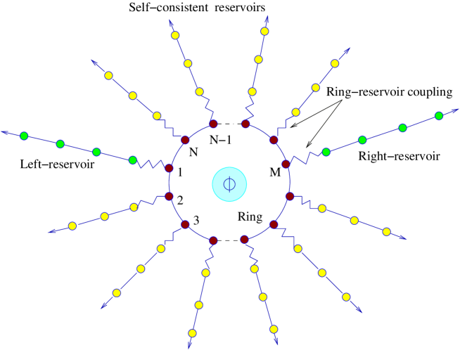
Figure 1: A schematic description of the model.

Following Ref.Dhar and Sen (2006); Roy and Dhar (2007), we get the steady state solution of the ring variables in Fourier domain,

$$\tilde{c}_{l}(\omega) = \sum_{m=1}^{N}~{}G^{+}_{lm}(\omega)~{}\tilde{\eta}_{m}(\omega)$$ (2)

$${\rm where}~{}~{}~{}\tilde{c}_{l}(\omega) = (1/2\pi)\int_{-\infty}^{\infty}dte^{i\omega t}c_{l}(t),~{}~{}~{}G^{+}=\frac{\hbar}{\gamma}Z^{-1},$$

$${\rm and}~{}~{}~{}Z_{lm} = \frac{\hbar}{\gamma}(\omega-\Sigma^{+}_{l})~{}\delta_{lm}+e^{-i\theta}\delta_{l,m-1}+e^{i\theta}\delta_{l,m+1}+e^{i\theta}\delta_{l1}\delta_{mN}+e^{-i\theta}\delta_{lN}\delta_{m1}~{}.$$

$G^{+}(\omega)$ is the Green’s function of the full system (ring and reservoirs) and for points on the ring can be written in the form $G^{+}(\omega)=[\omega-H_{r}/\hbar-\bar{\Sigma}^{+}]^{-1}$ where $\bar{\Sigma}^{+}$, defined by its matrix elements $\bar{\Sigma}^{+}_{lm}=\Sigma^{+}_{l}\delta_{lm}$, is a self-energy term modeling the effect of infinite reservoirs on the isolated single particle ring Hamiltonian $H_{r}$.  $\Sigma^{+}_{l}(t)=(\frac{\gamma_{l}^{\prime}}{\hbar})^{2}~{}g^{l+}_{1,1}(t)$ where $g^{l+}_{1,1}(t)$ is the single particle Green’s function of the lth reservoir at site 1. Here $\tilde{\eta}(\omega)$ is the noise characterising reservoir’s initial distribution. The effective ring Hamiltonian is $H_{r}+\hbar\bar{\Sigma}^{+}$ which can be shown to be non-Hermitian. We will use it to find bound states in a later section. Now one important point to notice is that, for $\theta$ not equal to an integral multiple of $\pi$, $Z_{lm}$ is not symmetric matrix. So the presence of magnetic flux $\phi$ breaks down the symmetric property of the $G^{+}(\omega)$ whenever $\phi$ is not equal to an integral multiple of $N{\phi}_{0}/2$. This is a consequence of the loss of the time reversal symmetry of the problem in the presence of magnetic flux.

In the present work we are interested in electron current from the reservoirs to the ring and also current in the ring. For this purpose we first define electron density operator on the ring sites and then use the continuity equation to get the corresponding current operators. Let us define $j_{l}$ as the electron current between sites $l~{},l+1$ on the ring and $j_{r-l}$ as the electron current from the ring to the $l^{\rm th}$ reservoir. These are given by the following expectation values:

$$j_{l} = \frac{ie\gamma}{\hbar}\langle~{}e^{i\theta}c_{l+1}^{\dagger}c_{l}-e^{-i\theta}c_{l}^{\dagger}c_{l+1}~{}\rangle$$

$$j_{r-l} = \frac{-ie\gamma_{l}^{\prime}}{\hbar}\langle~{}c_{l}^{\dagger}c_{1}^{l}-{c_{1}^{l}}^{{\dagger}}c_{l}~{}\rangle$$

where $e$ is the charge of the electron. Using the general solution in Eq. (2) and the noise-noise correlation Roy and Dhar (2007), we can do the above averaging and find

$$j_{l} = \sum_{m=1}^{N}\frac{-1}{2\pi}\int_{-\infty}^{\infty}d\omega\mathcal{F}_{lm}~{}(f_{l}-f_{m})$$ (3)

$$j_{r-l} = \sum_{m=1}^{N}\frac{1}{2\pi}\int_{-\infty}^{\infty}d\omega\mathcal{T}_{lm}~{}(f_{l}-f_{m})$$ (4)

$${\rm with}~{}~{}\mathcal{F}_{lm} = \frac{2\pi ie\gamma{\gamma^{\prime}_{m}}^{2}}{\hbar^{3}}~{}(~{}e^{i\theta}G^{+}_{lm}G^{-}_{ml+1}-e^{-i\theta}G^{+}_{l+1m}G^{-}_{ml}~{})~{}{\rho}_{m}$$

$${\rm and}~{}~{}\mathcal{T}_{lm} = \frac{4\pi^{2}e{\gamma^{\prime}_{l}}^{2}{\gamma^{\prime}_{m}}^{2}}{\hbar^{4}}~{}|G_{lm}^{+}|^{2}\rho_{l}\rho_{m}~{}~{},$$

where $G^{-}_{lm}={G^{+}_{ml}}^{*}$ and $f_{l}$ is the Fermi function. The chemical potentials of the reservoirs at the sites of the ring 1, M are specified by $\mu_{1}=\mu_{L}$ and $\mu_{M}=\mu_{R}$. Here we restrict ourselves at low temperature and linear response regime where the applied chemical potential difference $\Delta\mu=\mu_{R}-\mu_{L}$ is small i.e. $\Delta\mu\ll\mu_{L,R}$ and $k_{B}T\ll\mu_{L,R}$. For notational simplicity we choose: $\gamma_{l}=\gamma$ for $l=1,2...N$ and $\gamma^{\prime}_{l}=\gamma^{\prime}$ for $l=2,3...M-1,M+1,..N$. With this assumption, the reservoirs including source and drain will have the same Green’s function and density of states and we will use the notation $g^{l+}_{1,1}(\omega)=g^{+}(\omega)$ and $\rho_{l}(\omega)=\rho(\omega)$ Roy and Dhar (2007).

In the linear response regime, taking Taylor expansion of the Fermi functions $f(\omega,\mu_{l},T)$ about the mean value $\mu=(\mu_{L}+\mu_{R})/2$, Eqs. (3) and (4) reduce to the following set of equations:

$$j_{l} = \frac{-1}{2\pi\hbar}\sum_{m=1}^{N}\mathcal{F}_{lm}~{}(\mu_{l}-\mu_{m})$$ (5)

$$j_{r-l} = \frac{1}{2\pi\hbar}\sum_{m=1}^{N}\mathcal{T}_{lm}~{}(\mu_{l}-\mu_{m})~{}~{}~{}{\rm for}~{}~{}~{}l=1,2...N~{},$$ (6)

where $\mathcal{F}_{lm}$ and $\mathcal{T}_{lm}$ are evaluated at $\omega=\mu/\hbar$. These are linear equations in $\{\mu_{l}\}$ and are straightforward to solve numerically. In the next section we will consider the case of an open ring in the presence of uniform dephasing and dissipation. Later, we will study the persistent current in an asymmetric open ring in the absence of both magnetic flux and decoherence by external reservoirs.

III Extended Büttiker’s model for uniform dephasing in open ring enclosing magnetic flux

Before presenting results of uniform dephasing in the open ordered ring threaded by magnetic flux $\phi$, we first try to address the issue of, why we require an extension of Büttiker’s single probe model, apart from the construction of a more realistic microscopic model. In this section we work out all the results for a symmetric open ordered ring, i.e., the number of sites in the two arms of the ring between two contacts at 1 and $M$, are equal, or $N_{1}=N_{2}$. All the results remain unchanged for the asymmetric case from the physics point of view. Also we keep ideal leads at 1 and $M$, i.e., $\gamma_{1}^{\prime}=\gamma_{M}^{\prime}=\gamma$. We take a single Büttiker voltage probe and insert it in two positions of the open ring, once in the bulk of the arms between the two contacts, and then at the boundary of the arms. Next the chemical potential of this voltage probe is determined from the self-consistent condition of zero average electron current from this probe to the ring. We set from Eq. (6), $j_{r-l}=0$ where $l$ is the position of the Büttiker probe. Then the equation is solved numerically for chemical potential of the self-consistent reservoir with local density of states and total Green’s function as given in Appendix A. Finally we calculate the conductance $G(\phi)$ between two contacts at 1 and M from the same Eq. (6) for $j_{r-l}$ but with $l=1~{}{\rm or}~{}M$. In Fig. (2) we plot $G(\phi)$ with changing magnetic flux for two different postions of the Büttiker probe in the bulk or boundary of the open ring’s arms. In both cases coupling ${\gamma}^{\prime}$ of the probe with the ring is the same. Though conductance profiles for the two above stated cases are not much different qualitatively still a single probe dephases almost doubly when in the boundary than in the bulk. So there is distinct non-universality in the results from the context of quantity of dephasing with a single Büttiker probe depending on it’s position in the ring.

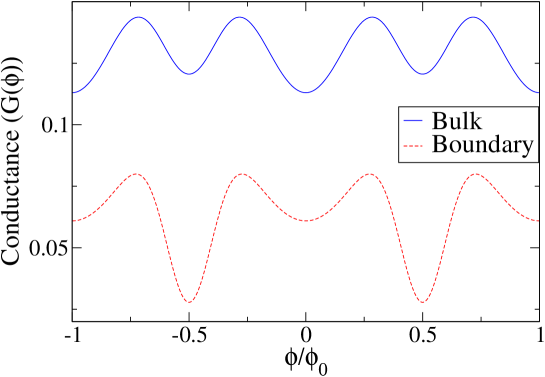
Figure 2: Plot of the conductance G($\phi$) of the open symmetric ring with single Büttiker probe. The total number sites in the ring, $N=20$ and ${\gamma}^{\prime}$=1.5 .

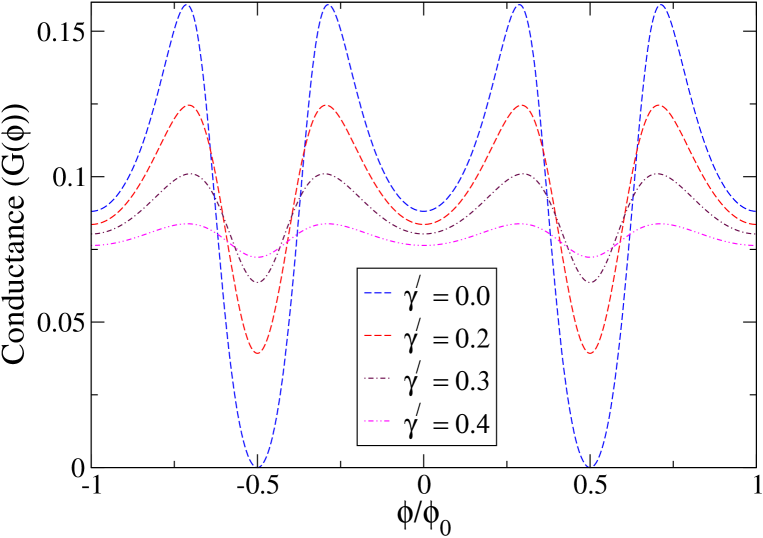
Figure 3: Plot of the Aharonov-Bohm oscillations of conductance G($\phi$) of the open symmetric ring with uniform dephasing for different strengths of coupling ${\gamma}^{\prime}$, with $N=20$ .

Now we work out the extended Büttiker’s model with all the sites between contacts 1 and $M$ being coupled to side reservoirs to simulate other degrees of freedom present in a real ring. Again to obtain the chemical potentials of the side reservoirs we fix the average electron current from these reservoirs to the ring to be zero independently. So we solve the following $N-2$ linear equations for $N-2$ unknown chemical potentials $\{\mu_{l}\}$,

$$j_{r-l}=0~{}~{}~{}{\rm for}~{}~{}~{}l=2,3,...M-1,M+1,...N.$$ (7)

Once the chemical potential profile of the side reservoirs is found, we use Eq. (6) with $l=1~{}{\rm or}~{}M$, to determine the electron current from the source to drain. First, we carry out both the above jobs numerically. In all the numerical results presented in this paper we set electrical charge and Planck constant $\hbar$ as unity. In Fig. (3) we plot conductance G($\phi$) as a function of enclosed magnetic flux for different values of the coupling ${\gamma}^{\prime}$ of the side reservoirs with the ring. Here we define conductance as the total current from the source to the drain divided by chemical potential difference between them, $\Delta\mu=\mu_{R}-\mu_{L}$. Clearly AB oscillations of conductance G($\phi$) decay with increasing decoherence parameter ${\gamma}^{\prime}$ indicating dephasing. Also the introduction of uniform dephasing does not destroy Onsager’s reciprocity relation i.e., $G(\phi)=G(-\phi)$. Using the similarity between different terms of the full Green’s function and $G_{lm}^{+}(\omega)|_{\phi}=G_{ml}^{+}(\omega)|_{-\phi}$, we can verify that under flux reversal the solutions of Eqs. (7) tranform as

$$\mu_{l}(\phi) = \mu_{1}+\mu_{M}-\mu_{l^{\prime}}(-\phi)~{}~{}~{}~{}~{}~{}{\rm for}~{}~{}~{}~{}1<l<M,$$ (8)

$$\mu_{l}(\phi) = \mu_{1}+\mu_{M}-\mu_{N+l^{\prime}}(-\phi)~{}~{}~{}~{}{\rm for}~{}~{}~{}~{}M<l<N,$$ (9)

where $l^{\prime}=M+1-l$. With these transformations and the above mentioned Green’s function properties, we see that the total current, i.e., conductance, remains invariant under $\phi\to-\phi$.

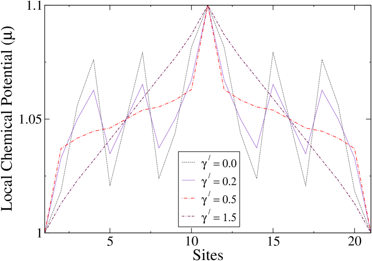
Figure 4: Plot of the local chemical potential profiles of the ring sites for different values of the decoherence parameter ${\gamma}^{\prime}$ with ${\phi}$ tends to zero, $N=20$ and site 21$\equiv$ site 1 .

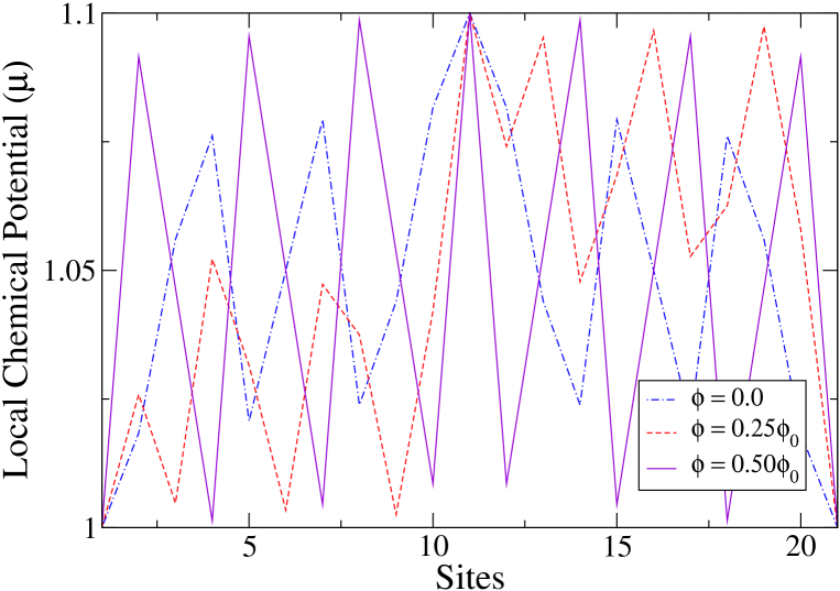
Figure 5: Plot of the local chemical potential profiles of the ring sites for different magnetic flux with ${\gamma}^{\prime}$ tends to zero, $N=20$ and site 21$\equiv$ site 1 .

As discussed earlier in the introduction, one elegant outcome of this extension is that, we can now evaluate local chemical potential profiles of the ring’s sites with changing magnetic flux by tuning ${\gamma}^{\prime}$ tends to zero. This is quite analogous to a four- probe measurement of a voltage drop in a nanoscale system de Picciotto et al. (2001). First we give in Fig. (4) solutions of the chemical potentials from Eqs. (7) with magnetic flux $(\phi)$ tends to zero. It shows large oscillations in the local chemical potential profile for small ${\gamma}^{\prime}$ and that become more and more flat with increasing ${\gamma}^{\prime}$. Finally the profile becomes completely linear for large ${\gamma}^{\prime}$, signalling Ohmic incoherent transport of electrons in this regime, which has been discussed in great detail in our earlier work Roy and Dhar (2007). The oscillations in the local chemical potential profile for tiny decoherence can be argued as due to the periodic geometry of the ring. A electron wave incident from the right lead gives two contributions to the current of the middle voltage probe measuring local chemical potential. One, there is direct transmission into the probe and another, a portion of the carriers which are transmitted past the left lead by travelling through the other arm of the ring and enter the voltage probe. It is the superpostion of these two interfering electron waves which determines transmission in the voltage probe. Following M. Büttiker Buttiker88 ; Buttiker89 we call it $phase$-$sensistive$ voltage measurement. For slightly larger dephasing, the flat behaviour of the chemical potential profile in the bulk of the arms and jumps at the contacts, is a signature of an intermediate regime between ballistic and Ohmic transport. This pattern is quite nicely explained using a simple persistent random walk model in our previous paper Roy and Dhar (2007). In Fig. (5) local chemical potential profiles of the ring with changing magnetic flux $\phi$ are given for the completely coherent case $(\gamma^{\prime}=0)$. For $\phi$ equal to an integer multiple of $\phi_{0}$, the chemical potential profiles are the same. Again for $\phi$ an integer multiple of $\phi_{0}/2$, the chemical potential profiles are similar. In both cases, the profiles are symmetric (mirror) about the contacts for the symmetric ring.

Now we derive an analytic expression for the $phase$-$sensitive$ local chemical potential profile Buttiker02 of the ring sites with changing magnetic flux as in Fig. (5). We couple a single Büttiker probe invasively (though the final result is insensitive to the coupling stregth $\gamma^{\prime}$) with a middle site of the open ring. We then determine the chemical potential ($\mu_{l}$) of the probe, i.e., the corresponding site, from the self consistent Eq. (6). Moving the probe over all middle sites of the ring we can evaluate the full $\{\mu_{l}\}$ profile in a compact form.

$$\mu_{l}=\frac{|G_{l1}^{+}|^{2}\mu_{L}+|G_{lM}^{+}|^{2}\mu_{R}}{|G_{l1}^{+}|^{2}+|G_{lM}^{+}|^{2}}~{}~{}~{}{\rm for}~{}~{}~{}l=2,3,...M-1,M+1,...N,$$ (10)

where $G_{l1}^{+}$ and $G_{lM}^{+}$ are given in Appendix A. This derivation will not work for the $\{\mu_{l}\}$ profile with uniform finite decoherence. The oscillations in the $\{\mu_{l}\}$ profile depends on the Fermi energy and the applied magnetic flux through the dispersion relation.

IV Persistent Current in open asymmetric ring: Role of closed ring’s eigenstates

In this section we investigate currents in a normal-metal ring connected with source and drain asymmetrically i.e. $N_{1}\not=N_{2}$. Asymmetry is very much required to achieve persistent current or current magnification effect in the open ring in the absence of magnetic flux. We find an analytic expression for conductance $G(\phi)$ between two contacts of the ring from Eq. (6) by evaluating the Green’s function as given in Appendix A. To find persistent current or circulating current in the ring, we have to know currents in both arms of the open ring separately. First we modify Eq. (5) to get current expressions $j_{u}~{}{\rm and}~{}j_{d}$ in the up and down arms respectively.

$$j_{u} = \frac{ie\gamma{\gamma^{\prime\prime}}^{2}}{\hbar^{4}}~{}(~{}e^{i\theta}G^{+}_{NM}G^{-}_{M1}-e^{-i\theta}G^{+}_{1M}G^{-}_{MN}~{}){\rho}~{}(\mu_{M}-\mu_{1})$$ (11)

$$j_{d} = \frac{-ie\gamma{\gamma^{\prime\prime}}^{2}}{\hbar^{4}}~{}(~{}e^{i\theta}G^{+}_{1M}G^{-}_{M2}-e^{-i\theta}G^{+}_{2M}G^{-}_{M1}~{}){\rho}~{}(\mu_{M}-\mu_{1})$$ (12)

with $\gamma^{\prime}_{1}=\gamma^{\prime}_{M}=\gamma^{\prime\prime}$ and $\gamma^{\prime}=0$. Whenever current in an arm of the asymmetric ring becomes larger than the total current $j$ between source and drain, there flows a circulating current in the ring exactly equal to the current in the other arm. This can be achieved by tuning the Fermi energy of the ring. The phenomenon of getting a larger current in the arms than the transport current is known as current magnification. The conductance $G(\phi)$ of the normal-metal ring between two contacts in the presence of magnetic flux is,

$$G(\phi)=\frac{2\pi e^{2}{\rho}^{2}{\gamma^{\prime\prime}}^{4}(-1)^{N-p}{|C^{0}_{1M}|}^{2}}{\hbar^{5}{|\Delta^{0}_{N}|}^{2}}$$ (13)

where $p,~{}{|C^{0}_{1M}|}^{2}~{}{\rm and}~{}|\Delta^{0}_{N}|$ are given in Appendix A. $G(\phi)$ is defined as $j=G(\phi)\Delta\mu/e$. Also we find from the expressions in Appendix A that $G(\phi)=G(-\phi)$. Similarly exact expressions of the currents $j_{u}~{}{\rm and}~{}j_{d}$ in the up and down arms of the ring can be evaluated. These expressions are quite long and not included here. In Fig. (6) we plot $j_{u},~{}j_{d}~{}{\rm and}~{}j$ with changing Fermi energy of an asymmetric ring with ideal leads $\gamma^{\prime\prime}=\gamma$ at the two contacts in the absence of magnetic flux. Clearly for some values of Fermi energy the current flows through the one arm of the open ring only whereas other arm is completely in an off condition. There are some special values of Fermi energy where the total transmission from source to drain goes to zero ($<10^{-10}$). Around these Fermi energy values the current magnification phenomenon arises. The asymmetric pattern of total transmission around these anti-resonances is referred to as Fano line shape.

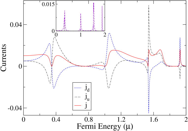
Figure 6: Plot of the currents in the two arms $j_{u}~{},~{}j_{d}$ and the total current $j$ in the asymmetric ring with ideal leads $\gamma^{\prime\prime}=\gamma$ in the absence of magnetic flux $\phi$. The inset shows the total current $j$ for tunnel barriers $\gamma^{\prime\prime}=0.3\gamma$. In both cases $N=18~{}{\rm and}~{}N_{1}:N_{2}=3:1$ .

We now determine the energy eigenvalues of the closed ring from the tight-binding Hamiltonian. Energy eigenvalues are $E_{m}=-2\gamma\cos(2\pi m/N)~{}{\rm with}~{}m=1,2..N$. For $N=18~{}{\rm and}~{}\gamma=1$, there are 8 doubly degenerate eigenvalues, $\pm$1.87939, $\pm$1.53209, $\pm$1, $\pm$0.347296 and two limiting values $\pm$2 . We find zero transmission points are exactly at these doubly degenerate eigen-energies. We suspect there exist bound states of the total Hamiltonian as the transmission goes to zero in the absence of an extended state from source to drain. We will show below using an effective Hamiltonian approach that indeed they are bound states embedded in the continuum of scattering states (BIC). Also different ratios between arms’ length, $N_{1}:N_{2}$, do change the transmission line shape pattern but not the antiresonance positions in the energy spectrum. In the inset of Fig. (6) we plot total current $j$ as a function of Fermi energy in the weak coupling limit $\gamma^{\prime\prime}<\gamma$. The transmission zeros at the doubly degenerate eigenvalues still survive but the two neighbored resonances around it almost merge together and their widths get reduced though the heights remain the same. Also radiation shifts of the positions of the resonant peaks relative to the energy eigenvalues of the closed ring are observed in this regime. In strong coupling limit $\gamma^{\prime\prime}>\gamma$, whereas anti-resonance points remain fixed, the resonance peaks expand.

$Effective~{}Hamiltonian~{}approach:$ Following Ref. Dhar and Sen (2006) the bound states are obtained as real solutions of the equation

$$[H_{r}+\hbar{\Sigma}^{+}_{L}(\omega)+\hbar{\Sigma}^{+}_{R}(\omega)]~{}|\psi\rangle=\lambda|\psi\rangle,$$ (14)

where ${\Sigma}^{+}_{L}(\omega)~{}{\rm and}~{}{\Sigma}^{+}_{R}(\omega)$ are self-energy corrections arising from the interaction of the ring with the left and right reservoirs respectively. Eigenstates of the tight-binding closed ring are given as

$$|\varphi_{m}\rangle=\sqrt{\frac{2}{N}}\sum_{j=1}^{N}\cos(\frac{2\pi mj}{N})|j\rangle.$$ (15)

Let us multiply $\langle\varphi_{m}|$ from the left of both sides of Eq. (14) and then introduce closure relation $\sum_{n=1}^{N}|\varphi_{n}\rangle\langle\varphi_{n}|=1$ for the isolated ring.

$$\langle\varphi_{m}|[H_{r}+\hbar{\Sigma}^{+}_{L}(\omega)+\hbar{\Sigma}^{+}_{R}(\omega)]\sum_{n=1}^{N}|\varphi_{n}\rangle\langle\varphi_{n}|\psi\rangle=\lambda\langle\varphi_{m}|\psi\rangle.$$ (16)

Using the definition of self-energies we get,

$$\sum_{n=1}^{N}\langle\varphi_{m}|\mathcal{H}_{eff}|\varphi_{n}\rangle\langle\varphi_{n}|\psi\rangle=\lambda\langle\varphi_{m}|\psi\rangle~{}~{}~{}{\rm for}~{}m=1,2...N,$$ (17)

$${\rm with} \langle\varphi_{m}|\mathcal{H}_{eff}|\varphi_{n}\rangle=E_{m}\delta_{mn}+g^{+}(\omega)[\frac{{\gamma^{\prime}_{1}}^{2}}{\hbar}\varphi^{\ast}_{m}(1)\varphi_{n}(1)+\frac{{\gamma^{\prime}_{M}}^{2}}{\hbar}\varphi^{\ast}_{m}(M)\varphi_{n}(M)],$$

where $\varphi_{n}(j)=\langle j|\varphi_{n}\rangle$. Eq. (17) ia a matrix eigenvalue equation with $\mathcal{H}_{eff}$ referred to as the non-Hermitian effective Hamiltonian in S-matrix theory for transmission Dittes00 ; Sardeev03 . Restricting the energy of the reservoirs’ electron in the conduction band i.e. $|\hbar\omega|<2\gamma$, we evaluate the eigenvalues of Eq. (17) numerically. The real values of $\lambda$ are precisely the doubly degenerate eigenvalues of the closed ring. So there exist bound states at the energy values of Fano antiresonances. Also a change in the strength or positions of the reservoir-ring couplings does not change the real eigenvalues of $\mathcal{H}_{eff}$. Only the complex eigenvalues get changed. This explains as to why the positions of the antiresonances remain same for the different ratios of the arms’ length, or with weak or strong couplings.

V Discussion

In the present work we have removed the sensitivity of dephasing by the external probe to its position at the bulk and the boundary of the ring’s arm in the Büttiker’s single probe model, by coupling every site of the open ring with self-consistent reservoirs. Of late the mesoscopic AB oscillations have served as a measuring device for different mechanisms of electron decoherence such as electron-electron scattering, and scattering off magnetic impurities wagner06 ; Pierre03 ; Pierre02 . Our extended model will be useful to understand the experiments where the decoherence in the ring occurs uniformly because of the interactions of conducting electrons with the other degrees of freedom present in the system. There are other perfectly valid models for uniform dephasing arun02 ; brouwer97 . Still our extension is closer to experiments as here the coupling between the ring and the environment is direct and easily tunable. Recently the resistance of single-wall carbon nanotubes have been studied Gao05 in a four-probe configuration with noninvasive voltage electrodes. They have found that the four-probe resistance fluctuates and can even become negative at cryogenic temperature due to quantum-interference effects generated by elastic scatterers Buttiker89 in the nanotube. With recent progress in experiments with quantum rings Fuhrer01 we believe that it is possible to detect the local chemical potential oscillations in the open ring as predicted in the present paper. Here we should mention that differences between $phase$-$sensitive$ and $phase$-$insensitive$ measurements are drastic for an effectively single-channel transmission problem compare to multichannel conductor where it depends on the particular arrangement of probe-coupling Buttiker89 . It is also required further attention to investigate effects of static disorder (elastic scatterer) and electron-electron interaction on the local chemical potential oscillations. There is good scope to study the mutual effect of disorder and dissipation in dissipative open quantum systems by introducing disorder in the ring Hamiltonian through our extended model in the quantum Langevin equation approach.

The Fano antiresonance occurs because of the interference of a discrete autoionized state with a continuum. Here we have shown for the single channel transport in the asymmetric open ring, the antiresonances occur exactly at the doubly degenerate energy eigenstates of the closed ring in the absence of evanescent modes. Also by finding the real eigenvalues of the non-Hermitian effective Hamiltonian we predict the existence of the BIC at these Fano antiresonance energy values. Recently some more studies have found the BIC in an AB ring and in a double cavity electron waveguide Bulgakov06 ; Ordonez06 . Here we emphasize that in case of single channel transport the total transmission of an open symmetric ring never goes to zero in the absence of magnetic flux. Finally bound states do not contribute directly in the transport for non-interacting systems. However as suggested by a mean field calculation in Ref.Dhar and Sen (2006), they may affect the current via affecting the local density in the presence of electron-electron interactions. It will be interesting to see that how the interactions between the electrons affect the transmission zeros in the open asymmetric ring.

VI acknowledgments

The author wants to thank Abhishek Dhar and N. Kumar for many discussions on the phenomenon of decoherence, and to R. Srikanth for a critical reading of the manuscript. The author would also like to express his gratitude to M. Büttiker for his critical remarks on the manuscript and K. Ensslin for a helpful discussion on the possibility of experimental realisation of the chemical potential oscillations in quantum rings.

Appendix A Evaluation of Green’s Function

The full Green’s function is given as $G^{+}_{lm}=(\hbar/\gamma)Z^{-1}_{lm}$ where $Z$ is a near circulant matrix with off-diagonal terms $Z_{N1}=Z_{l~{}l+1}=e^{-i\theta}~{}{\rm for}~{}l=1,2...N-1$ and $Z_{1N}=Z_{l-1~{}l}=e^{i\theta}~{}{\rm for}~{}l=2,3...N$. The diagonal terms are given by:

$$Z_{11} = Z^{+}_{MM}=A(\omega)=\frac{\hbar}{\gamma}~{}[\omega-\frac{{\gamma^{\prime\prime}}^{2}}{\hbar^{2}}g^{+}(\omega)]~{}~{}~{}{\rm with}~{}~{}\gamma^{\prime}_{1}=\gamma^{\prime}_{M}=\gamma^{\prime\prime}~{},$$

$$Z_{ll} = B(\omega)=\frac{\hbar}{\gamma}~{}[\omega-\frac{{\gamma^{\prime}}^{2}}{\hbar^{2}}g^{+}(\omega)]~{}~{}~{}{\rm for}~{}~{}l=2,3...M-1,M+1...N~{}.$$ (18)

Now using the method of Ref. Roy and Dhar (2007) to determine inverse and determinant of the tri-diagonal matrix, we can find required inverse and determinant of the near circulant matrix $Z$ through simple but tedious algebra.

$$\Delta_{N} = \left((A-2\cosh\alpha)^{2}(\cosh[N\alpha]-\cosh[p\alpha])-4{\sinh}^{2}\alpha((-1)^{N}\cos[N\theta]-\cosh[N\alpha])\right.$$ (19)

$$+ \left.4\sinh\alpha\sinh[N\alpha](A-2\cosh\alpha)\right)/(2{\sinh}^{2}\alpha)~{}~{}~{}{\rm with}~{}~{}e^{\pm\alpha}=\frac{B}{2}\pm(\frac{B^{2}}{4}-1)^{1/2}.$$

with $p=N_{2}-N_{1}$. Similarly, the co-factor can be evaluated following the above trick. Here we find first $C_{1M}$ and calculate ${|C_{1M}|}^{2}$ which is relevant to determine conductance $G(\phi)$ of the asymmetric ring between the drain and source contacts.

$${|C_{1M}|}^{2} = 2\left[\cosh N\alpha_{R}\cosh p\alpha_{R}-\cos N\alpha_{I}\cos p\alpha_{I}+(-1)^{N}\{\cos N\theta~{}(\cos p\alpha_{I}\cosh N\alpha_{R}-\cos N\alpha_{I}\right.$$ (20)

$$\left.\cosh p\alpha_{R})+\sin N\theta~{}(\sin p\alpha_{I}\sinh N\alpha_{R}-\sin N\alpha_{I}\sinh p\alpha_{R})\}\right]/(\cosh 2\alpha_{R}-\cos 2\alpha_{I}).~{}$$

where $\alpha_{R}~{}{\rm and}~{}\alpha_{I}$ are respectively real and imaginary part of $\alpha$. For $\gamma^{\prime}=0$, the real part of $\alpha$ vanishes and the coefficient of $\sin N\theta$ in ${|C_{1M}|}^{2}$ also disappears. We denote, ${{|C_{1M}|}^{2}}_{\gamma^{\prime}=0}$ by ${|C^{0}_{1M}|}^{2}$ and $|{\Delta_{N}}|_{\gamma^{\prime}=0}$ by $|{\Delta}^{0}_{N}|$.

Finally we evaluate the Green’s function of Eq. (10), where a single Büttiker probe is coupled to a middle site (l) of the open ring. Here again $Z_{11}=Z^{+}_{MM}=A(\omega)$, but all other diagonal terms are $\hbar\omega/\gamma$ except $Z_{ll}=B(\omega)$. The off-diagonal terms remain the same as before. Following the above method we calculate the Green’s function ($l<M$)

$$G^{+}_{l1} = \frac{(-1)^{l+1}\hbar}{2\gamma\Delta^{\prime}_{N}\sinh^{2}\alpha^{\prime}}\left[e^{i(l-1)\theta}\{B(\cosh[(N-l+1)\alpha^{\prime}]-\cosh[(r+1)\alpha^{\prime}])-2\cosh[(N-l)\alpha^{\prime}]\right.$$

$$\left.+\cosh[r\alpha^{\prime}]+\cosh[(r+2)\alpha^{\prime}]\}+(-1)^{N}e^{i(l-N-1)\theta}(\cosh[l\alpha^{\prime}]-\cosh[(l-2)\alpha^{\prime}])\right]$$

$${\rm with}~{}~{}~{}e^{\pm\alpha^{\prime}}=\frac{\hbar\omega}{2\gamma}\pm(\frac{{\hbar}^{2}{\omega}^{2}}{16\gamma^{2}}-1)^{1/2}~{}~{},$$

where $r=N-2M+l$. In this case, we do not require to determine $\Delta^{\prime}_{N}$, the determinant of $Z$, as it gets cancelled in Eq. (10). Similarly $G^{+}_{lM}$ can be evaluated.

References

- Büttiker, Imry and Landauer (1983) M. Büttiker, Y. Imry and R. Landauer, Phys. Lett. 96A, 365 (1983).
- Gefen, Imry and Azbel (1984) Y. Gefen, Y. Imry and M. Ya. Azbel, Phys. Rev. Lett. 52, 139 (1984).
- Lévy et al. (1990) L. P. Lévy, G. Dolan, J. Dunsmuir and H. Bouchiat, Phys. Rev. Lett.64, 2074 (1990).
- Chandrasekhar et al. (1991) V. Chandrasekhar, R. A. Webb, M. J. Brady, M. B. Ketchen, W. J. Gallagher and A. Kleinsasser, Phys. Rev. Lett. 67, 3578 (1991).
- Webb et al. (1985) R. A. Webb, S. Washburn, C. P. Umbach, R. B. and Laibowitz, Phys. Rev. Lett. 54, 2696 (1985).
- (6) O. Hod, R. Baer and E. Rabani., Phys. Rev. Lett. 97, 266803 (2006).
- Büttiker (1985) M. Büttiker, Phys. Rev. B 32, 1846 (1985).
- Büttiker (1986) M. Büttiker, Phys. Rev. B 33, 3020 (1986).
- Pilgram (2006) S. Pilgram, P. Samuelsson, H. Förster and M. Büttiker, Phys. Rev. Lett. 97, 066801 (2006).
- Förster (2007) H. Förster, P. Samuelsson, S. Pilgram and M. Büttiker, Phys. Rev. B75, 035340 (2007).
- Bolsterli et al. (1970) M. Bolsterli, M. Rich and W. M. Visscher, Phys. Rev. A 4, 1086 (1970).
- Dhar and Roy (2006) A. Dhar and D. Roy, J. Stat. Phys. 125, 801 (2006), eprint cond-mat/0606465.
- (13) K. B. Efetov, Phys. Rev. Lett. 74, 2299 (1995).
- (14) P. W. Brouwer and C. W. J. Beenakker, Phys. Rev. B 55, 4695 (1997).
- de Picciotto et al. (2001) R. de Picciotto, H. L. Stormer, L. N. Pfeiffer, K. W. Baldwin and K. W. West, Nature (London) 411, 51 (2001).
- (16) A. M. Jayannavar and P.Singha Deo, Phys. Rev. B 51, 10175 (1995).
- (17) S. Bandopadhyay, P. S. Deo and A. M. Jayannavar, Phys. Rev. B 70, 075315 (2004).
- Dhar and Sriram Shastry (2003) A. Dhar and B. Sriram Shastry, Phys. Rev. B 67, 195405 (2003).
- Dhar and Sen (2006) A. Dhar and D. Sen, Phys. Rev. B 73, 085119 (2006).
- Roy and Dhar (2007) D. Roy and A. Dhar, Phys. Rev. B 75, 195110 (2007), eprint cond-mat/0611274.
- (21) M. Büttiker, IBM J. Res. Dev.32, 317 (1988).
- (22) M. Büttiker, Phys. Rev. B 40, 3409 (1989).
- (23) M. Büttiker, PRAMANA-J.Phys.58, 241 (2002).
- (24) F.-M. Dittes, Phys. Rep. 339, 215 (2000).
- (25) A. F. Sadreev and I. Rotter, J. Physics A Mathematical General, 36, 11413 (2003).
- (26) K. Wagner, D. Neumaier, M. Reinwald, W. Wegscheider and D. Weiss, Phys. Rev. Lett. 97, 206804 (2006).
- (27) F. Pierre, A. B. Gougam, A. Anthore, H. Pothier, D. Esteve and N. Birge, Phys. Rev. B 68, 085413 (2003).
- (28) F. Pierre and N. O.Birge, Phys. Rev. Lett. 89, 206804 (2002).
- (29) C. Benjamin and A. M. Jayannavar, Phys. Rev. B 65, 153309 (2002).
- (30) B. Gao, Y. F. Chen, M. S. Fuhrer, D. C. Glattli and A. Bachtold, Phys. Rev. Lett. 95, 196802 (2005).
- (31) A. Fuhrer, S. Lüscher, T. Ihn, T. Heinzel, K. Ensslin, W. Wegscheider, and M. Bichler, Nature (London)413, 822 (2001).
- (32) E. N. Bulgakov, K. N. Pichugin, A. F. Sadreev and I. Rotter, JETP Letters, 84, 430 (2006).
- (33) G. Ordonez, K. Na and S. Kim, Phys. Rev. A 73, 022113 (2006).