Abstract

In the context of the AdS/CFT correspondence we calculate the induced stress tensor of static dipoles (electric-electric and electric-magnetic) in a strongly coupled ${\cal N}=4$ SYM gauge theory, by solving the linearized Einstein equation with Maldecena string as a source. Analytic expressions are given for the far-field and a near-field close to one charge, and compared to what one has in weak coupling. The result can be compared to lattice results for QCD-like theories in a deconfined but strongly coupled regime.

Department of Physics and Astronomy, SUNY Stony-Brook, NY 11794

1 Introduction

AdS/CFT correspondence [1] relates conformal $\cal N$=4 supersymmetric Yang-Mills theory (CFT) with string theory in $AdS_{5}\times S_{5}$ space-time. Large number of colors $N\rightarrow\infty$ and ’t Hooft coupling $\lambda=g_{YM}^{2}N\rightarrow\infty$ further lead to the classical supergravity regime (weak coupling) for the latter, putting the CFT into a strong coupling regime. In the decade since its invention, this correspondence became an indispensable theoretical tool, providing multiple interesting results about a strongly coupled regime of $\cal N$=4 supersymmetric gauge theory.

Among the earliest were calculation of the energy of a static electric dipole [2], based on a shape of “pending string” held at the AdS boundary at the positions of two static fundamental quarks, separated by distance $L$. For further reference we will need the EOM of the string

$$x_{z}=-\frac{z^{2}}{\sqrt{z_{m}^{4}-z^{4}}}$$ (1)

where $z_{m}$ is the maximal string extension into z direction. We will also use notation $L/2=x_{m}\approx 0.60z_{m}$.

The resulting potential

$$E=-\frac{4\pi^{2}\left(g_{YM}^{2}N\right)^{1\over 2}}{\Gamma\left(1\over{4}\right)^{4}L}$$ (2)

has the famous factor $\sqrt{\lambda}$ (instead of $\lambda$ in the weak coupling Coulomb law. Soon this calculation was extended to include magnetic objects (monopoles and dyons) by Minahan [3], which can be viewed as an endpoints of the appropriate $D_{1}$ branes on the boundary. We will continue to discuss puzzles related with the dipoles in the next subsection.

Naively one may interpret this answer by thinking of a strongly coupled vacuum as a dielectric medium, with a dielectric constant given by the ratio of the strong coupling result to the zero order Coulomb: potential

$$\epsilon={V_{Coulomb}\over V_{Maldacena}}={\sqrt{\lambda}\Gamma(1/4)^{4}\over 8\pi^{3}}\approx.636\sqrt{\lambda}$$ (3)

Although in a very qualitative sense this idea is not wrong, it is certainly not literally true. A proof of that are the calculations to be reported below, which shows that the stress tensor distribution in space is very different from that in weak coupling. Of course, this is to be expected, as the strongly coupled vacuum recieves nonperturbative modification from the fields, leading to a nonlinear response.

Now, a decade later, there is a spike of activity of using AdS/CFT to understand properties of the deconfined phase of QCD, known as Quark-Gluon Plasma (QGP) [4]. A number of phenomenological considerations lead to a conjecture [5] that QGP to be in a ’strongly coupled’ regime (sQGP) at temperatures not too high above the deconfinement temperature $T=(1-2)T_{c}$. It is in this domain where RHIC experiments at Brookhaven found a “perfect liquid” properties of sQGP. Among AdS/CFT-based works devoted to it are calculations of the energy loss [6] and stress tensor imprint [7] of the moving objects in thermal CFT plasma. Those are quite spectacular, providing in particular a compete picture justifying another hydrodynamical phenomenon, a “conical flow” in Mach direction around the jet.

Lattice studies of sQGP have also indicated features indicative of a strong coupling regime. Those most relevant for this work obviously are studies of static charge pairs (electric or magnetic). Large deviation from a perturbative picture of a screened Coulombic potential are observed at $T$ above the deconfinement transition $T_{c}$. More specifically, many features at $T>1.5Tc$ suggest a “quasi-conformal” regime, in which all dimensional quantities (e.g. normalized energy density $\epsilon/T^{4}$) show weak $T$-dependence.

(Even larger deviations from perturbative approach – the Debye-screened charges – are seen for static dipoles at $T_{c}<T<1.5T_{c}$. Here the entropy and potential energy associated with the string has very large part, linearly growing with distance in some range, see e.g. [10]. The question whether flux tubes – remnants of confining strings – can continue to exist in a plasma phase was recently studied in [11].)

More generally, the dynamics of electric and magnetic gauge fields in a strongly coupled plasma remains very poorly understood. In particular, it has been suggested that sQGP contains large component of magnetically charged quasiparticles – monopoles and dyons, see [12, 13]. Studies of the energy distribution in plasma induced by static dipoles have been extensively done at zero temperature, demonstrating existence of quantum confining string: unfortunately similar calculations at $T>T_{c}$ are not yet available. One may wander whether the deconfined QCD-like theories in those regimes are or are not similar to the vacuum of $\cal{N}$=4 Gauge Theory at strong coupling.

These ideas motivated our present calculation, in which we calculate stress tensor “imprint” of static dipoles in AdS/CFT. A simple diagrammatic picture of what is calculated is provide by Fig.2. Apart of the solutions themselves, to be given below in different regimes, there are few particular issues which would like to investigate:
(i) How the dipole is seen at large distances $r\rightarrow\infty$? What is the power of distance and its angular distribution? Can it be related to expected behavior of electric and scalar fields?
(ii) What is the field near one of the charges? Can a non-singular part corresponding to the fields of a second charge and polarization cloud be identified?
(iii) Is there a visible remnant of the Matsubara string, or a picture rather is of two polarization clouds? In particular, what is the r.m.s. transverse size $\sqrt{<y_{\perp}^{2}>}$ at $\lvert y\rvert=0$ (the middle point)?
(iv) We will also consider an electric-magnetic pair: our main interest in that is to see if there is some nontrivial features related with electric-magnetic field interaction.

1.1 Strongly coupled versus weakly coupled dipoles

One issue discussed in literature (after AdS/CFT potentials been calculated) was whether some kind of diagram resummation can get the reduction of the coefficient, from $\sim\lambda$ to $\sim\sqrt{\lambda}$. Semenoff and Zarembo[14] have found that one can do so using ladder diagrams. Shuryak and Zahed [15] have noticed that such ladder diagrams in a strongly coupled regime imply a very short correlation time between colors of both charges

$$\delta t\sim L/\lambda^{1/4}$$ (4)

which will be crucial for understanding of the large-distance field below.

The “imprint” of the pending string on the boundary was first addressed by Callan and Guijosa [16], who had calculated an “image” due to scalar (dilaton) field propagating in the bulk. The boundary operator associated with a dilaton is $trF^{2}$. Our work is very close to theirs, except that we calculate much more cumbersome graviton propagation instead of a scalar one, to get the boundary stress tensor.

Their main results was a distribution of scalar density at large distances from a dipole $r\gg L$ (i) has the form

$$trF^{2}(r)\sim L^{3}/r^{7}$$ (5)

and (ii) is spherically symmetric. Both are very different from what one finds for the shape of the electric field of a weakly coupled electric dipole, which has (i) power 6 and (ii) has a characteristic dipole energy distribution $(3cos^{2}(\theta)+1)$ ($\theta$ is polar angle from a dipole direction). Our calculation to be reported also will show power 7 but will have more complicated angular distribution.

The reason why the power is 7 rather than 6 was explained by Klebanov,Maldacena and Thorn [17]. Imagine Euclidean time and perturbative diagram, in which perturbative field of each charge can be written as a time integral over a propagator, from a world line of a charge to an observation point: it produces power 6. The nontrivial point is that in strongly coupled regime color time correlation [15] mentioned above require both charges to emit quanta at the $same$ time; this changes a double time integral into a single one, adding one more power of the distance.

2 Solving the linearized Einstein equations in $AdS_{5}$

As is clear from Introduction, the source of gravity in our problem are strings extended into the AdS space. Naturally those are considered to be weak sources, so we will linearize the Einstein equations (with $\Lambda=6$)

$$R_{\mu\nu}-{1\over{2}}Rg_{\mu\nu}+\Lambda g_{\mu\nu}=-{\kappa}^{2}T_{\mu\nu}$$ (6)

(6) and solve for small deviations from the unperturbed $AdS_{5}$ metric.

We choose to start with another form of (6):

$$R_{\mu\nu}+\left(\Lambda-\frac{-{\kappa}^{2}T-\Lambda d}{2-d}g_{\mu\nu}\right)=-{\kappa}^{2}T_{\mu\nu}$$ (7)

with $d=5$ Linearizion of the above gives:

$${\delta}R_{\mu\nu}-4{\delta}g_{\mu\nu}={\delta}S_{\mu\nu}$$ (8)

where ${\delta}S_{\mu\nu}=-{\kappa}^{2}\left({\delta}T_{\mu\nu}-\frac{{\delta}T}{3}g_{\mu\nu}\right)$

We denote weak gravity perturbation as ${\delta}g_{\mu\nu}=h_{\mu\nu}$ and use an axial gauge in which the following components vanish $h_{z\mu}=0\;(\mu=z,t,x^{1},x^{2},x^{3})$. We use the usual Poincare coordinates for the AdS metric:

$$ds^{2}=\frac{-dt^{2}+d{\vec{x}}^{2}+dz^{2}}{z^{2}}$$ (9)

and set the AdS radius $L_{ADS}$ to 1.

Expressing the modifications of curvature ${\delta}R_{\mu\nu}$ in terms of $h_{\mu\nu}$, (see Appendix.A for a brief derivation) we get the following equations

$${1\over 2}h_{,z,z}-{1\over{2z}}h_{,z}={\delta}S_{zz}$$ (10)

$${1\over 2}\left(h_{,m}-h_{m}\right)_{,z}={\delta}S_{zm}$$ (11)

$${1\over 2}\square h_{mn}-2h_{mn}+{z\over 2}h_{mn,z}-{1\over 2}\left(h_{m,n}+h_{n,m}\right)+{1\over 2}\left(h_{,m,n}-\Gamma_{mn}^{z}h_{,z}\right)={\delta}S_{mn}$$ (12)

where we have defined $h=g^{{\lambda}\sigma}h_{{\lambda}\sigma}$, $h_{m}=g^{{\lambda}\sigma}h_{{\lambda}m,\sigma}$, $\square=z^{2}\left(-\partial_{t}^{2}+\partial_{{\vec{x}}}^{2}+\partial_{z}^{2}\right)$, and from now on latin indices stand for 4 boundary coordinates $(m,n=t,x^{1},x^{2},x^{3})$.

We could in principle solve for $h$ from (10), the result of which can help to solve for $h_{m}$ from (11). Finally solve for $h_{mn}$ with $h$,$h_{m}$ plugged in (12). However, we choose to do it in a slightly different way: As (11) is first order in $z$, it is only a constraint equation. With the boundary condition: $h_{mn}=0$(thus $h=0$,$h_{m}=0$) at $z=0$, we obtain

$$h_{m}=h_{,m}-2\int_{0}^{z}{\delta}S_{zm}dz$$ (13)

(10) is second order in $z$, but it gives also a constraint when combined with (12): Denoting $\left(m,n\right)$ as the mn component of (12), $-\left(t,t\right)+\Sigma_{i}\left(x^{i},x^{i}\right)$ gives:

$${1\over 2}h_{,z,z}-{7\over{2z}}h_{,z}=-{\delta}S_{tt}+\Sigma_{i}{\delta}S_{x^{i}x^{i}}-2\int\left(-{\delta}S_{zt,t}+\Sigma_{i}{\delta}S_{zx^{i},x^{i}}\right)dz$$ (14)

Combining (10) and (14), we obtain the solution for $h$

$$h={1\over 3}\int_{0}^{z}dz\cdot z\left({\delta}S_{zz}+{\delta}S_{tt}-\Sigma_{i}{\delta}S_{x^{i}x^{i}}+2\int_{0}^{z}dz\left(-{\delta}S_{zt,t}+\Sigma_{i}{\delta}S_{zx^{i},x^{i}}\right)\right)$$ (15)

With $h$ obtained from (15) and $h_{m}$ eliminated, (12) becomes a closed eqn for remaining components:

$${1\over 2}\square h_{mn}-2h_{mn}+{z\over 2}h_{mn,z}=s_{mn}$$ (16)

where a “generalized source” is $s_{mn}={\delta}S_{mn}-\int_{0}^{z}\left({\delta}S_{zm,n}+{\delta}S_{zn,m}\right)dz+{1\over 2}h_{,m,n}+{1\over 2}\Gamma_{mn}^{z}h_{,z}$

The source terms created by the string are obtained from the Nambu-Goto action of the string in a standard way

$$S_{NG}=-\frac{1}{2\pi\alpha^{\prime}}\int d^{2}\sigma\int d^{5}x\sqrt{-detg}{\delta}^{\left(5\right)}\left(x-X\left(\sigma\right)\right)$$

$${\delta}T^{\mu\nu}=\frac{2{\delta}S_{NG}}{\sqrt{-G}{\delta}G_{\mu\nu}}$$

$$=\frac{-1}{\sqrt{-G}2\pi\alpha^{\prime}}\int d^{2}\sigma{\delta}^{\left(5\right)}\left(x-X\left(\sigma\right)\right)\partial_{\alpha}X^{\mu}\partial_{\beta}X^{\nu}g^{\beta\alpha}$$ (17)

here we use $G_{\mu\nu}$ and $g_{\alpha\beta}$ to denote AdS metric and induced metric respectively.

The string world sheet can be described by

$$x^{1}=x\left(t,z\right),\>x^{2}=x^{3}=0$$ (18)

The resulting source is as follows (we use the order of coordinate indices in the following 5-d matrices as $t,z,x^{1},x^{2},x^{3}$ and all absent entries are zeros)

$${\delta}S_{\mu\nu}=\frac{-{\kappa}^{2}z}{2\pi\alpha^{\prime}}{\delta}\left(x^{1}-x\right){\delta}\left(x^{2}\right){\delta}\left(x^{3}\right)\frac{1}{\sqrt{1+x_{z}^{2}-x_{t}^{2}}}$$

$$\begin{pmatrix}{{2x_{t}^{2}+x_{z}^{2}+1}\over 3}&x_{t}x_{z}&-x_{t}&&\\ x_{t}x_{z}&{{x_{t}^{2}+2x_{z}^{2}-1}\over 3}&-x_{z}&&\\ -x_{t}&-x_{z}&{{x_{t}^{2}-x_{z}^{2}+2}\over 3}&&\\ &&&-{2\over 3}\left(x_{t}^{2}-x_{z}^{2}-1\right)&\\ &&&&-{2\over 3}\left(x_{t}^{2}-x_{z}^{2}-1\right)\end{pmatrix}$$ (19)

With (16),(15) and (2), we can solve for $h_{mn}$, provided any explicit profile of the string. We will do this for three different string profiles separately in the following sections, and extract the corresponding stress tensors.

3 The stress tensor of a static quark

As a warm up, we will start with the case of a straight string, which corresponds to a single quark in $\cal N$=4 SYM. The string profile is simply $x\left(t,z\right)=0$. Substitute in (2), we obtain:

$${\delta}S_{\mu\nu}=\frac{-{\kappa}^{2}z}{2\pi\alpha^{\prime}}{\delta}\left(x^{1}\right){\delta}\left(x^{2}\right){\delta}\left(x^{3}\right)\begin{pmatrix}{1\over 3}&&&&\\ &-{1\over 3}&&&\\ &&{2\over 3}&&\\ &&&{2\over 3}&\\ &&&&{2\over 3}\end{pmatrix}$$ (20)

Static source leads to the metric perturbation $h_{mn}$ which is time-independent. Performing a Fourier transform $h_{mn}^{k}=\int h_{mn}e^{i{\vec{k}}{\vec{x}}}d^{3}x$ we convert the PDE (16) to an ODE:

$${1\over 2}z^{2}\left(h_{mn,z,z}^{k}-k^{2}h_{mn}^{k}\right)-2h_{mn}^{k}+{z\over 2}h_{mn,z}^{k}=s_{mn}^{k}$$ (21)

An upper index k will be used below to indicate a Fourier transformed quantity.

$S_{\mu\nu}^{k}$ is just $S_{\mu\nu}$ without delta functions. $h^{k}$ and $s_{\mu\nu}^{k}$ have simple forms displayed as follows:

$$h^{k}=-{2\over 9}\frac{-{\kappa}^{2}}{2\pi\alpha^{\prime}}z^{3}$$ (22)

$$s_{mn}^{k}=\frac{-{\kappa}^{2}}{2\pi\alpha^{\prime}}\left[\begin{pmatrix}{2\over 3}&&&\\ &{1\over 3}&&\\ &&{1\over 3}&\\ &&&{1\over 3}&\end{pmatrix}z+\begin{pmatrix}0&&&\\ &&&\\ &&k_{m}k_{n}&\\ &&&\end{pmatrix}{z^{3}\over 9}\right]$$ (23)

The equation is Bessel type and can be dealt with using a Green function built out of such functions. Instead we consider a more general equation with arbitrary power of $z$ in the source

$${1\over 2}z^{2}\left(h_{mn,z,z}^{k}-k^{2}h_{mn}^{k}\right)-2h_{mn}^{k}+{z\over 2}h_{mn,z}^{k}=c_{n}z^{n}$$ (24)

which is directly solvable in terms of Meijer-G funcion and hypergeometric function:

$$h_{mn}^{k}=I_{2}(kz)\left(C_{2}+G_{1,3}^{2,1}\left(\frac{k^{2}z^{2}}{4}\Big{|}^{1}_{{n\over 2}+1,{n\over 2}-1,0}\right)\frac{2^{n-1}}{k^{n}}\right)$$

$$+K_{2}(kz)\left(C_{1}-_{1}F_{2}\left({}^{{n\over 2}+1}_{{n\over 2}+2,3}\Big{|}\frac{k^{2}z^{2}}{4}\right){\frac{k^{2}z^{n+2}}{4n+8}}\right)$$ (25)

The constants $C_{1}$ and $C_{2}$ are to be fixed by boundary conditions. One of the condition is the metric perturbation vanishes at AdS boundary, i.e. $h_{mn}^{k}=0$ at $z=0$, which fixes $C_{1}=0$. The other boundary condition proposed in [9] for thermal AdS is incoming metric perturbation at the horizon. However in our case, we need a different boundary condition due to the absence of horizon in AdS. Since $h^{k}$ grows as $z^{3}$ in the present case, while $h_{mn}^{k}$ show possible exponential growth at large z. It is natural to propose no exponential growth at $z=\infty$ as the boundary condition.

At large z, only the first term containing $I_{2}(kz)$ is dominant, the boundary condition becomes:

$$C_{2}+\frac{2^{n-1}}{k^{n}}G_{1,3}^{2,1}\left(\frac{k^{2}z^{2}}{4}\Big{|}^{1}_{{n\over 2}+1,{n\over 2}-1,0}\right)=0$$

The asymptotic of Meijer-G function ($z\rightarrow\infty$) gives:

$$G_{1,3}^{2,1}\left(\frac{k^{2}z^{2}}{4}\Big{|}^{1}_{{n\over 2}+1,{n\over 2}-1,0}\right)\rightarrow\Gamma\left({n\over 2}+1\right)\Gamma\left({n\over 2}-1\right)$$

which finally fixes $C_{2}=-\frac{c_{n}2^{n-1}}{k^{n}}\Gamma\left({n\over 2}+1\right)\Gamma\left({n\over 2}-1\right)$. Applying it to our source $s_{mn}=c_{1}z+c_{3}z^{3}$, where $c_{1}$ and $c_{3}$ are matrix-valued (the indices are suppressed here), we have $C_{2}={\pi\over k}c_{1}-{3\pi\over k^{3}}c_{3}$

The stress tensor of the corresponding boundary CFT is proportional to the coefficient of $z^{2}$ term, which we denote as $Q_{mn}$ throughout this paper, in small z expansion of $h_{mn}$. The precise relation can be obtained from (36) of [7], which in our case is simply (with $L_{ADS}=1$):

$$T_{mn}=\frac{2}{{\kappa}^{2}}Q_{mn}$$ (28)

Note $G_{1,3}^{2,1}\left(\frac{k^{2}z^{2}}{4}\Big{|}^{1}_{{n\over 2}+1,{n\over 2}-1,0}\right)$ and ${}_{1}F_{2}\left({}^{{n\over 2}+1}_{{n\over 2}+2,3}\Big{|}\frac{k^{2}z^{2}}{4}\right)z^{n+2}$ contains only odd power of z for odd $n$, thus does not contribute to $Q_{mn}$. We have

$$Q_{mn}={1\over 8}k^{2}C_{2}$$ (29)

Reinstate the factor $L_{ADS}^{2}$, together with the relation $\frac{L_{ADS}^{2}}{\alpha^{\prime}}=\sqrt{{\lambda}}$, we have the final stress tensor:

$$T_{mn}^{k}=\frac{-\sqrt{{\lambda}}}{\pi}\frac{k^{2}}{8}\left[\begin{pmatrix}{2\over 3}&&&\\ &{1\over 3}&&\\ &&{1\over 3}&\\ &&&{1\over 3}\end{pmatrix}{\pi\over k}-\begin{pmatrix}0&&&\\ &&&\\ &&k_{m}k_{n}&\\ &&&\end{pmatrix}{\pi\over{3k^{3}}}\right]$$ (30)

It is easy to verify the stress tensor above is traceless $T_{mn}\eta^{mn}=0$, which is a consequence of conformal invariance. It also satisfies the conservation of energy and momentum $k^{m}T_{mn}=0$. In doing inverse Fourier transform, we find the k-integrals are not well-defined. One trick is to introduce a regulator $e^{-ak}\left(a>0\right)$ to the integral, and take the limit $a\rightarrow 0$ in the final answer. We end up with the following result:

$$T_{mn}=\frac{-\sqrt{{\lambda}}}{\pi}\frac{1}{8\pi}\left[-{2\over{3r^{4}}}\begin{pmatrix}1&&&\\ &1&&\\ &&1&\\ &&&1\end{pmatrix}+\begin{pmatrix}0&&&\\ &&&\\ &&y_{m}y_{n}&\\ &&&\end{pmatrix}{4\over{3r^{6}}}\right]$$ (31)

where r is the distance from the quark. The ${1\over r^{4}}$ power is obvious by dimension. Let us recall the result obtained in [16]

$${\cal O}_{F^{2}}={1\over{4g_{YM}^{2}}}trF^{2}+\cdots={1\over{2g_{YM}^{2}}}tr(-E^{2}+B^{2})+\cdots$$

$$={1\over{32\pi^{2}}}\frac{\sqrt{{\lambda}}}{r^{4}}$$ (32)

While in our case, the $T_{00}$ component gives

$$T_{00}={1\over{2g_{YM}^{2}}}tr(E^{2}+B^{2})+\cdots$$

$$={1\over{12\pi^{2}}}\frac{\sqrt{{\lambda}}}{r^{4}}$$ (33)

In both (3) and (3), the dots represent contributions from scalars and gluinoes. If we assume the magnetic field is not present, the difference in the two operators implies significant contribution are received from the scalars and gluinoes.

4 The stress tensor image of static electric dipole

Now we turn to the Maldacena’s pending string, the ends of which attached to a quark and antiquark, corresponding to a static electric dipole. The string profile $x(z)$ is double-valued. We use $\pm x(z)\>(x(z)>0)$ to denote two halves of the string. The EOM can be integrated to give $x(z)$ in terms of elliptic integrals. We will not refer to explicit form until the end of the calculation.

The source term and its Fourier transformed version are a bit complicated:

$${\delta}S_{\mu\nu}=\frac{-{\kappa}^{2}z}{2\pi\alpha^{\prime}}{\delta}\left(x^{1}-x(z)\right){\delta}\left(x^{2}\right){\delta}\left(x^{3}\right)\frac{1}{\sqrt{1+x_{z}^{2}}}$$

$$\begin{pmatrix}{{x_{z}^{2}+1}\over 3}&&&&\\ &{{2x_{z}^{2}-1}\over 3}&-x_{z}&&\\ &-x_{z}&{{-x_{z}^{2}+2}\over 3}&&\\ &&&{{2x_{z}^{2}+2}\over 3}&\\ &&&&{{2x_{z}^{2}+2}\over 3}\end{pmatrix}+(x\rightarrow-x)$$ (34)

$${\delta}S_{\mu\nu}^{k}=\frac{-{\kappa}^{2}z}{2\pi\alpha^{\prime}}\frac{2}{\sqrt{1+x_{z}^{2}}}\biggl{[}\begin{pmatrix}{{x_{z}^{2}+1}\over 3}&&&&\\ &{{2x_{z}^{2}-1}\over 3}&&&\\ &&{{-x_{z}^{2}+2}\over 3}&&\\ &&&{{2x_{z}^{2}+2}\over 3}&\\ &&&&{{2x_{z}^{2}+2}\over 3}\end{pmatrix}\cos(k_{1}x)$$

$$+\begin{pmatrix}0&0&0&&\\ 0&0&-x_{z}&&\\ 0&-x_{z}&0&&\\ &&&0&0\\ &&&0&0\end{pmatrix}i\sin(k_{1}x)\biggr{]}$$ (35)

It is understood that the source term vanishes for $z>z_{m}$. (15) and (16) gives:

$$h(z<z_{m})={1\over 3}\frac{-{\kappa}^{2}}{2\pi\alpha^{\prime}}F(z)\;$$ (36)

$$h(z>z_{m})={1\over 3}\frac{-{\kappa}^{2}}{2\pi\alpha^{\prime}}\left(F(z_{m})+{1\over 2}(z^{2}-z_{m}^{2})G(z_{m})\right)\;$$

$$s_{mn}^{k}(z<z_{m})=\frac{-{\kappa}^{2}}{2\pi\alpha^{\prime}}\biggl{[}{1\over 3}E_{1}(z)\begin{pmatrix}1&&&\\ &-1&&\\ &&2&\\ &&&2\end{pmatrix}+{1\over 3}E_{2}(z)\begin{pmatrix}1&&&\\ &-1&&\\ &&2&\\ &&&2\end{pmatrix}$$

$$+H(z)\begin{pmatrix}0&&&\\ &2k_{1}&k_{2}&k_{3}\\ &k_{2}&&\\ &k_{3}&&\end{pmatrix}-{1\over 3}F(z)\begin{pmatrix}0&&&\\ &&&\\ &&\frac{k_{m}k_{n}}{2}&\\ &&&\end{pmatrix}+\frac{F^{\prime}(z)}{6z}\begin{pmatrix}-1&&&\\ &1&&\\ &&1&\\ &&&1\end{pmatrix}\biggr{]}\;$$ (37)

$$s_{mn}^{k}(z>z_{m})=\frac{-{\kappa}^{2}}{2\pi\alpha^{\prime}}\biggl{[}H(z_{m})\begin{pmatrix}0&&&\\ &2k_{1}&k_{2}&k_{3}\\ &k_{2}&&\\ &k_{3}&&\end{pmatrix}-{1\over 3}\left(F(z_{m})+{1\over 2}(z^{2}-z_{m}^{2})G(z_{m})\right)$$

$$\begin{pmatrix}0&&&\\ &&&\\ &&\frac{k_{m}k_{n}}{2}&\\ &&&\end{pmatrix}+\frac{G(z_{m})}{6}\begin{pmatrix}-1&&&\\ &1&&\\ &&1&\\ &&&1\end{pmatrix}\biggr{]}\;$$ (38)

with

$$E_{1}(z)=\frac{2z}{\sqrt{1+x_{z}^{2}}}x_{z}^{2}\cos(k_{1}x)$$

$$E_{2}(z)=\frac{2z}{\sqrt{1+x_{z}^{2}}}\cos(k_{1}x)$$

$$F(z)=\int_{0}^{z}\frac{-4\cos(k_{1}x)}{\sqrt{1+x_{z}^{2}}}z^{2}dz+\int_{0}^{z}dz\left(z\int_{0}^{z}\frac{-4\sin(k_{1}x)}{\sqrt{1+x_{z}^{2}}}zk_{1}x_{z}dz\right)$$

$$G(z_{m})=\int_{0}^{z_{m}}\frac{-4\sin(k_{1}x)}{\sqrt{1+x_{z}^{2}}}zk_{1}x_{z}dz$$

$$H(z)=\int_{0}^{z}\frac{2z\sin(k_{1}x)}{\sqrt{1+x_{z}^{2}}}x_{z}dz$$ (39)

With the explicit expression of $s_{mn}^{k}$, we can build the general solution to (16):

$$h_{mn}^{k}=I_{2}(kz)C_{2}+K_{2}(kz)C_{1}+2\left(I_{2}(kz)\int_{z_{m}}^{z}\frac{s_{mn}^{k}(z)K_{2}(kz)}{z}dz-K_{2}(kz)\int_{z_{m}}^{z}\frac{s_{mn}^{k}(z)I_{2}(kz)}{z}dz\right)$$ (40)

At large z, no exponential growth condition requires $C_{2}+2\int_{z_{m}}^{\infty}\frac{s_{mn}^{k}(z)K_{2}(kz)}{z}dz=0$. The convergence of the integral is ensured by $K_{2}(kz)$ in the integrand . At small z, $s_{mn}^{k}\sim O(z)$ while $I_{2}(kz)\sim O(z^{2})$ the integral containing $I_{2}(kz)$ is finite as z approach 0, therefore the boundary condition gives: $C_{1}-2\int_{z_{m}}^{0}\frac{s_{mn}^{k}(z)I_{2}(kz)}{z}dz=0$.

In order to extract the stress tensor, we need to collect $z^{2}$ terms. It is helpful to write down the series expansion of the two integrals

$$\int_{z_{m}}^{z}\frac{s_{mn}^{k}(z)I_{2}(kz)}{z}dz=a_{0}+a_{1}z+\cdots$$ (41)

$$\int_{z_{m}}^{z}\frac{s_{mn}^{k}(z)K_{2}(kz)}{z}dz={b_{-1}\over z}+b_{0}+\cdots$$ (42)

The coefficient of $z^{2}$ is given by: $Q_{mn}={1\over 8}k^{2}C_{2}+{k^{2}\over 4}b_{0}$. Note $C_{1}$ does not appear in the expression We may also write it as

$$Q_{mn}^{k}=-{k^{2}\over 4}\int_{z_{m}}^{\infty}\frac{s_{mn}^{k}(z)K_{2}(kz)}{z}dz+{k^{2}\over 4}\lim_{{\epsilon\rightarrow 0}}\left(\int_{z_{m}}^{\epsilon}\frac{s_{mn}^{k}K_{2}(kz)}{z}dz-{b_{-1}\over\epsilon}\right)$$ (43)

We could proceed in momentum space. However it turns out to be much easier and illustrating to do inverse Fourier transform and continue in configuration space from now on.

A nice property of Fourier transform is ${\cal F}^{-1}(F(k)G(k))=\int f(x)g(y-x)dx$. Identifying the source dependent $s_{mn}^{k}$ as $F(k)$, the inverse Fourier transform of which gives $f(x)$. Correspondingly, each $G(k)$ is transformed to $g(y-x)$. The latter can be interpreted as a propagator from a point on the source $x$ to a point on the boundary $y$. With this in mind, we define the following propagator:

$$P_{s}({\vec{y}}-{\vec{x}})=\frac{1}{(2\pi)^{3}}\int k^{2}K_{2}(kz)e^{-i{\vec{k}}{\vec{x}}}d^{3}k={15\over{4\pi}}\frac{z^{2}}{\left(z^{2}+r^{2}\right)^{7\over 2}}$$ (44)

Let us take a moment to worry about the term involving $b_{-1}$. By analyzing small z behavior of $s_{mn}$ and $I_{2}(kz)$, we find $b_{-1}=\frac{\#}{k^{2}}$. Inverse Fourier transform of ${k^{2}\over 4}b_{-1}$ is not well-defined. Again we introduce the same regulator $e^{-ak}$ as in the previous section. We find a vanishing result after taking the limit $a\rightarrow 0$

Finally, we can write the stress tensor in a very short form:

$$Q_{mn}=-{1\over 4}\int_{z_{m}}^{\infty}dz\int\frac{s_{mn}(z,{\vec{x}})P_{s}({\vec{y}}-{\vec{x}})}{z}d^{3}x$$

$$+{1\over 4}\int_{z_{m}}^{0}dz\int\frac{s_{mn}(z,{\vec{x}})P_{s}({\vec{y}}-{\vec{x}})}{z}d^{3}x$$ (45)

Before proceeding with the calculation, we would like to make few general comments: (i) The trace of the stress tensor is given by the coefficient of $z^{4}$ term of $h$. From (36), we find that $h\sim F(z)$ at small z does $not$ contain $z^{4}$ term, therefore we expect the final stress tensor to be $traceless$, which is also required by conformal invariance. (ii) The divergence of the stress tensor $\partial_{{\lambda}}T_{{\lambda}m}$ turns out to be the the coefficient of $z^{4}$ term of $h_{m}$. From (13) and (36) we conclude $\partial_{{\lambda}}T_{{\lambda}m}=\frac{\sqrt{{\lambda}}}{\pi}{1\over{2z_{m}^{2}}}\left({\delta}(x^{1}-x_{m})-{\delta}(x^{1}+x_{m})\right){\delta}(x^{2}){\delta}(x^{3}){\delta}_{m1}$. The divergence is non-vanishing only for $m=x^{1}$ at the end points of the string where the quark and antiquark are placed. It corresponds to a pair of antiparallel forces which hold quark and antiquark, preventing them from falling onto each other. This will be another general condition to be satisfied by the stress tensor.

4.1 Far field

With (4) at hand, we first calculate the stress tensor in region far from the dipole. The inverse Fourier transforms of $s_{mn}$ are linear combinations of those of $E_{1},E_{2},F,G,H$. Such terms as $k_{m}H$ can be replaced by $i{\partial_{x_{m}}}H=-i{{\overleftarrow{\partial}}_{x_{m}}}H=i{{\overleftarrow{\partial}}_{y_{m}}}$. In the first identity, we use partial integration so that the derivative only acts on the propagators (we indicate this with a left arrow on top of the derivative). The second identity is due to $P_{s}=P_{s}({\vec{y}}-{\vec{x}})$. Similarly, $k_{m}k_{n}F\rightarrow-{\overleftarrow{\partial}}_{x_{m}}{\overleftarrow{\partial}}_{x_{n}}F\rightarrow-{\overleftarrow{\partial}}_{y_{m}}{\overleftarrow{\partial}}_{y_{n}}F$

We list the back-transformed result of $E_{1},E_{2},F,G,H$ here:

$$E_{1}=\frac{z^{5}}{z_{m}^{2}\sqrt{z_{m}^{4}-z^{4}}}{\delta}(x^{2}){\delta}(x^{3}){\delta}(x^{1}-x(z))+(x^{1}\rightarrow-x^{1})$$ (46)

$$E_{2}=\frac{z\sqrt{z_{m}^{4}-z^{4}}}{z_{m}^{2}}{\delta}(x^{2}){\delta}(x^{3}){\delta}(x^{1}-x(z))+(x^{1}\rightarrow-x^{1})$$ (47)

$$F={4\over{z_{m}^{2}}}{\delta}(x^{2}){\delta}(x^{3})\frac{-(z^{2}-z_{1}^{2})(z_{m}^{4}-3z_{1}^{4})}{4z_{1}^{2}}\theta(z-z_{1})+(x^{1}\rightarrow-x^{1})$$ (48)

$$G={4\over{z_{m}^{2}}}{\delta}(x^{2}){\delta}(x^{3})\left(-\frac{z_{m}^{4}-3z_{1}^{4}}{2z_{1}^{2}}\theta(z-z_{1})+\frac{z_{m}^{4}-z_{1}^{4}}{2z_{1}}{\delta}(z-z_{1})\right)+(x^{1}\rightarrow-x^{1})$$ (49)

$$H=-{1\over{z_{m}^{2}}}{\delta}(x^{2}){\delta}(x^{3})\frac{z_{1}\sqrt{z_{m}^{4}-z_{1}^{4}}}{i}\theta(z-z_{1})-(x^{1}\rightarrow-x^{1})$$ (50)

with $z_{1}=z_{1}(x^{1})\,(0<x^{1}<x_{m})$, the inverse function of $x(z)$. Contribution from negative $x^{1}$ is included in the second term for each function. Note $E_{1},E_{2},F,G$ are symmetric in $x^{1}$, while $H$ is antisymmetric.

In order to obtain the far field stress tensor, we need to perform a large $\lvert y\rvert$ expansion of the stress tensor. Note the y-dependence enters the stress tensor via the propagator, we can do a large $\lvert y\rvert$ expansion on the propagator in the second term since $z<z_{m}\ll\lvert y\rvert$. While for the first integral, z extending to infinity, we need to do the integral first before a valid expansion is possible. Fortunately this time the source has very simple z-dependence: $s_{mn}(z)=\#+\#z^{2}$. The rest of the calculation is straight forward. After collecting all terms, we find the first nontrivial result appears at the order ${1\over{\lvert y\rvert^{7}}}$. The power again agree with the result of $trF^{2}$ obtained in [16]. We list the stress tensor as follows (up to the order ${1\over{\lvert y\rvert^{7}}}$):

$$T_{00}={1\over 4}\frac{-\sqrt{{\lambda}}}{\pi}\frac{15}{4\pi}\left(\frac{a_{G}(7y_{1}^{2}-y^{2})}{12\lvert y\rvert^{9}}+\left({a_{E1}\over 3}+{a_{E2}\over 3}+{a_{F}\over 6}\right){1\over{\lvert y\rvert^{7}}}\right)$$ (51)

$$T_{0m}=0$$ (52)

$$T_{mn}={1\over 4}\frac{-\sqrt{{\lambda}}}{\pi}\frac{15}{4\pi}\biggl{[}\left(-7a_{H}+{7\over 6}a_{G}\right)\begin{pmatrix}2y_{1}&y_{2}&y_{3}\\ y_{2}&&\\ y_{3}&&\end{pmatrix}\frac{y_{1}}{\lvert y\rvert^{9}}+{2\over 3}\left(a_{E1}+a_{E2}\right){\delta}_{mn}{1\over{\lvert y\rvert^{7}}}$$

$$-\left(a_{E1}+{a_{G}\over 6}-2a_{H}\right)\begin{pmatrix}1&0&0\\ 0&&\\ 0&&\end{pmatrix}{1\over{\lvert y\rvert^{7}}}-\left({7a_{F}\over 6}-{7a_{G}\over 12}\right)\frac{y_{m}y_{n}}{\lvert y\rvert^{9}}-{21a_{G}\over 4}\frac{y_{m}y_{n}y_{1}^{2}}{\lvert y\rvert^{11}}\biggr{]}$$ (53)

with

$$a_{G}=2\int_{0}^{x_{m}}G(z_{m})\left(x^{1}\right)^{2}dx^{1}=-0.7189z_{m}^{3}$$

$$a_{F}=2\int_{0}^{x_{m}}F(z_{m})dx^{1}=-0.9585z_{m}^{3}$$

$$a_{H}=2\int_{0}^{x_{m}}H(z_{m})x^{1}dx^{1}=0.1797z_{m}^{3}$$

$$a_{E1}=\int_{z_{m}}^{0}E_{1}(z)dz=-0.7189z_{m}^{3}$$

$$a_{E2}=\int_{z_{m}}^{0}E_{2}(z)dz=-0.4793z_{m}^{3}$$

We can verifiy explicitly that the stress tensor is traceless and divergence-free at this order.

Now we proceed to analysis of the results, describing which features are general and should be expected and which of them are qualitatively new.

A vanishing energy flux (Poynting vector) $T_{0m}=0$ is related with zero magnetic field expected for static electric configuration. Indeed, a time reversal would change the sign of the magnetic field and the Poynting vector, but leaves the problem invariant.

Having said that, we by no means imply that the only field in question is the electric field. Indeed, vacuum polarization should include all other fields of the theory, and perturbatively we know that all color fields of the theory – gluinoes and scalars – should contribute, to charge polarization density as well as to the energy we calculate. However, a very simplistic view of the scalars based on $(\partial_{\mu}\phi)^{2}$ Lagrangian would produce the same distributions as a vector field, since that can be viewed as just generated by another scalar field $A_{0}$.

The obvious point of comparison is stress tensor distribution for a perturbative dipole. Its electric field

$$E_{m}(y)=({g^{2}\over 4\pi})\left({y_{m}-(L/2)e_{m}\over|y_{m}-(L/2)e_{m}|^{3}}-{y_{m}+(L/2)e_{m}\over|y_{m}+(L/2)e_{m}|^{3}}\right)$$ (55)

leads to stress tensor which is at large distances $\sim L^{2}/y^{6}$. The result we obtain is $\sim L^{3}/r^{7}$: the difference is due to the a phenomenon of “short-time-color-locking” [15, 17] we already discussed in the Introduction. Perhaps another way to explain it is to say that a scalar density, induced by a dipole, is large in all the volume $\sim L^{3}$.

Let us now comment on the angular distribution. Perturbative dipole field at large distances contains the first power of the dipole vector: thus its angular momentum is 1. Energy density constructed out of this field, obviously has only angular momenta 2 and 0, or powers of $cos^{n}(\theta)$ with $n=0,2$. Stress tensor also contains such components, but also terms of the type $T_{mn}\sim y_{m}y_{n}(\vec{L}\vec{y})^{2}$. Looking at our result we find that indeed no other angular structures appeared. This is to be expected, as electric field is still the only vector field of the theory. The angular distribution of the far field energy is compared to the perturbative result in Fig.1: although there is tendency to a more spherical distribution (like obtained for scalar density [16]), the peaks in the dipole directions are still there.

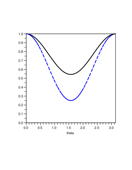
Figure 1: (Color online) The far field energy distribution in polar angle $\theta(cos(\theta)=y_{1}/\lvert y\rvert)$, normalized at zero angle. Solid (black) line is our result, compared to the perturbative result $(3cos^{2}+1)/4$ given by the dashed (blue) line.

One more simple case to discuss is the stress tensor on a line connecting the charges: by symmetry transverse component of the field $\vec{E}_{\perp}=0$ and only $E_{x}$ remains. The Maxwellian tensor then should satisfy $T_{22}=T_{33}=-T_{11}=T_{00}$: and the result we obtain does not satisfy it. We thus see once again, that gluino and scalar parts of the stress tensor $must$ contribute to the far field asymptotic in question.

4.2 A field near one charge

Next we would like to study the stress tensor near one of the charge. For this purpose, we make a shift of variables $y_{1}\rightarrow y_{1}+x_{m},\,y_{2}\rightarrow y_{2},\,y_{3}\rightarrow y_{3}$, and consider small $\lvert y\rvert$ behavior of the stress tensor.

It is clear from the single charge result(31) the stress tensor will blow up as $\lvert y\rvert\rightarrow 0$, so to the leading order in $\lvert y\rvert$, we may focus on its divergent part only.

Let us recall the basic expression for the stress tensor:

$$Q_{mn}=-{1\over 4}\int_{z_{m}}^{\infty}dz\int\frac{s_{mn}(z,{\vec{x}})P_{s}({\vec{y}}-{\vec{x}})}{z}d^{3}x$$

$$+{1\over 4}\int_{z_{m}}^{0}dz\int\frac{s_{mn}(z,{\vec{x}})P_{s}({\vec{y}}-{\vec{x}})}{z}d^{3}x$$ (56)

As $\lvert y\rvert\rightarrow 0$, the first term is finite($z>z_{m}$), which we ignore as discussed above. While the propagator in the second term $P_{s}={15\over{4\pi}}\frac{z^{2}}{\left(z^{2}+r^{2}\right)^{7\over 2}}$ contains a singularity at $z=0,\,r=0$, which leads to a possible divergence in stress tensor(unless the source provide enough powers of z). We can also claim the divergence is from integration at small z. Since the integral involving $s_{mn}$ and $P_{s}$ cannot be done analytically, a careful analysis is needed to obtain the leading terms in Laurent expansion of the stress tensor.

We first use the common factor ${\delta}(x^{2}){\delta}(x^{3})$ in the source to simplify the propagator:

$$r^{2}=(y_{1}+x_{m}-x^{1})^{2}+(y_{2}-x^{2})^{2}+(y_{3}-x^{3})^{2}=(y_{1}-\Delta x)^{2}+y_{2}^{2}+y_{3}^{2}$$

$$=r_{0}^{2}-2y_{1}\Delta x+\Delta x^{2}$$

with $r_{0}^{2}=y_{1}^{2}+y_{2}^{2}+y_{3}^{2}$, $\Delta x=x^{1}-x_{m}$. Then the propagator can be expanded in $\Delta x^{1}$:

$$P_{s}={15\over{4\pi}}\left(\frac{z^{2}}{\left(z^{2}+r_{0}^{2}\right)^{7\over 2}}-7\frac{z^{3}}{\left(z^{2}+r_{0}^{2}\right)^{9\over 2}}y_{1}\Delta x^{1}+\cdots\right)$$ (57)

Note the leading term of the propagator does not depend on $x^{1},x^{2},x^{3}$. A similar trick is used as in the case of far field: $k_{m}=-i{\overleftarrow{\partial}}_{x_{m}}=i{\overleftarrow{\partial}}_{y_{m}}$. The second identity is due to $P_{s}=P_{s}({\vec{y}}-{\vec{x}})$. If only the leading order result of the stress tensor is needed, we perform the x-integral with the source, keeping the smallest power in z(As we argued before smaller power of z corresponds to larger term in expansion of the stress tensor):

$$\int E_{1}d^{3}x\sim\frac{z^{5}}{z_{m}^{4}}$$

$$\int E_{2}d^{3}x\sim z$$

$$\int Fd^{3}x\sim-z_{m}^{2}\int(z^{2}-z_{1}^{2})\theta(z-z_{1})dx^{1}=-{2\over 3}z^{3}$$

$$\int{F^{\prime}\over z}d^{3}x\sim-2z_{m}^{2}\frac{z}{z_{1}^{2}}\theta(z-z_{1})dx^{1}=-2z$$

$$\int-iHd^{3}x\sim z_{1}\theta(z-z_{1})dx^{1}=\frac{z^{4}}{4z_{m}^{2}}$$

Convolute the above results with the leading order propagator, we find they give the following divergence:

$$E_{1}\rightarrow ln(r_{0})$$

$$E_{2},{F^{\prime}\over z}\rightarrow{1\over r_{0}^{4}}$$

$$F\rightarrow{1\over r_{0}^{2}}$$

$$iH\rightarrow{1\over r_{0}}$$

Therefore the leading order result is given by $E_{2},{F^{\prime}\over z}$ and $F$. The last also give ${1\over r_{0}^{4}}$ when combined with the double derivatives in the coefficient. Collecting all the contributions, we find the leading near field contribution, which is of course precisely the stress tensor of a single charge (31)

$$T_{mn}^{LO}=\frac{-\sqrt{{\lambda}}}{\pi}\frac{1}{8\pi}\biggl{[}-{2\over{3r_{0}^{4}}}\begin{pmatrix}1&&&\\ &1&&\\ &&1&\\ &&&1\end{pmatrix}+\begin{pmatrix}0&&&\\ &&&\\ &&y_{m}y_{n}&\\ &&&\end{pmatrix}{4\over{3r_{0}^{6}}}\biggr{]}$$ (58)

The aim now is to extend the analysis to the next order correction to (58). Note the correction from the source will give at least $O(z^{4})$ correction, while that from the propagator is of $O(\Delta x^{1})\sim z_{1}^{3}\sim z^{3}$, with an additional $z^{2}+r_{0}^{2}$ in the denominator. As a result, we can keep the leading order source but care about the correction from the propagator when necessary. Finally we find the next order correction to the stress tensor is from the LO source $E_{2},F,{F^{\prime}\over z}$ convoluted with the NLO correction to the propagator $-7\frac{z^{3}}{(z^{2}+r_{0}^{2})^{9\over 2}}y_{1}\Delta x^{1}$, as well as the leading result from $iH$. We display the correction to the near field as follows:

$$T_{{mn}}^{NLO}=\frac{-\sqrt{{\lambda}}}{\pi}\frac{1}{12\pi}\frac{1}{z_{m}^{2}}\biggl{[}{y_{1}\over{6r_{0}^{3}}}\begin{pmatrix}5&&&\\ &8&&\\ &&8&\\ &&&8\end{pmatrix}-\begin{pmatrix}0&&&\\ &2y_{1}&y_{2}&y_{3}\\ &y_{2}&&\\ &y_{3}&&\end{pmatrix}\frac{4}{3r_{0}^{3}}$$

$$-\begin{pmatrix}0&&&\\ &&&\\ &&y_{m}y_{n}&\\ &&&\end{pmatrix}\frac{y_{1}}{2r_{0}^{5}}\biggr{]}$$ (59)

We can also verify the stress tensor at this order is traceless and divergence-free.

Let us now analyze the results and compare it with expectations. In general one can expect that close to the charge there is a singular electric field $E^{sing}\sim 1/r_{0}^{2}$ plus a finite field induced by all other charges.

$$E_{i}E_{j}\approx E^{sing}_{i}E_{j}^{sing}+E^{sing}_{i}E_{j}^{reg}+E^{sing}_{j}E_{i}^{reg}+...$$ (60)

The scalar field in weak coupling add the same distributions.

If the vacuum would be a simple dielectric, both the singular and regular field would be just free fields times the dielectric constant (3), and the relative correction be the same. Let us see whether this idea works or not. In weak coupling the correction to $T_{00}$ is $1-2(y_{1}r)/L^{2}$ while our strong coupling result gives

$${T_{00}\over T_{00}^{LO}}=1-{(y_{1}r)\over z_{m}^{2}}\approx 1-0.34{2(y_{1}r)\over L^{2}}$$ (61)

The sign and the structure of the local field is the same, while the magnitude is additionally reduced by about a factor 1/3. What we learn from this comparison, once again, is that although a strongly coupled vacuum of the theory works as a polarizable dielectric qualitatively, this is not true literally.

4.3 Is there a visible trace of the string?

Another interesting question is the transverse distribution of energy. In particular we calculate the r.m.s.: $\sqrt{<y_{2}^{2}>}=\left(\frac{\int T_{00}y_{2}^{2}dy_{2}}{\int T_{00}dy_{2}}|_{y_{1}=y_{3}=0}\right)^{1\over 2}$, which characterizes the transverse energy distribution on the middle plane between the quark-antiquark pair.

$$T_{00}\sim Q_{00}={1\over 4}\int_{\infty}^{0}dz\int\frac{s_{00}(z,{\vec{x}})P_{s}({\vec{y}}-{\vec{x}})}{z}d^{3}x$$ (62)

$$s_{00}(z<z_{m})\sim\frac{E_{1}(z)}{3}+\frac{E_{2}(z)}{3}-\frac{F^{\prime}(z)}{6z}$$

$$s_{00}(z>z_{m})\sim-\frac{G(z_{m})}{6}$$

Note y-dependence enters only through the propagator $P_{s}$, we can do the $y_{2}$ integral with the propagator first, then convolute the result with the source $s_{00}$. The rest of the calculation is straight forward. We will skip the details and only give the result: $\sqrt{<y_{2}^{2}>}\approx 0.41z_{m}$, while half the size of the dipole is ${L\over 2}\approx 0.60z_{m}$. The r.m.s. is about ${1\over 3}$ of the dipole size, smaller than the perturbative result ${\sqrt{<y_{2}^{2}>}={L\over 2}}$.

In order to make the trace of string clear, we would like to rewrite (4) in a more physical form. This is done by defining: $s^{h}_{mn}=s_{mn}-S_{mn}$, then we have

$$Q_{mn}=-{1\over 4}\int_{0}^{\infty}dz\int\frac{S_{mn}(z,{\vec{x}})P_{s}({\vec{y}}-{\vec{x}})}{z}d^{3}x$$

$$-{1\over 4}\int_{0}^{\infty}dz\int\frac{s^{h}_{mn}(z,{\vec{x}})P_{s}({\vec{y}}-{\vec{x}})}{z}d^{3}x$$ (63)

The first piece is sourced by the original string $S_{mn}$, while the second piece corresponds to contribution from $s^{h}_{mn}$. Since the latter is obtained from $S_{\mu\nu}$ via (15) and (13). The transform from $S_{\mu\nu}$ to $s^{h}_{mn}$ can be interpreted as a bulk-to-bulk propagator, which is then attached to the bulk-to-boundary propagator $P_{s}$ to contribute to the stress tensor. We schematically illustrate the two contributions in Fig.2

Figure 2: (color online) Schematic demonstration of the pending string and the propagators of stress tensor. The source is at the point $A$ integrated over string, it either (a) goes directly to the observation point $y$ via bulk-to-boundary propagates(dashed line) , or (b) first transforms to $s^{h}_{mn}$ in some other point $B$ via bulk-to-bulk propagator(dash-dotted line), then goes to the observation point

We use the component $T_{00}$ as an example to study the relative contribution from the two pieces:

$$Q_{00}^{1}=-{1\over 4}\int_{0}^{\infty}dz\int\frac{S_{mn}(z,{\vec{x}})P_{s}({\vec{y}}-{\vec{x}})}{z}d^{3}x$$

$$={-1\over 6}\int_{0}^{z_{m}}\frac{z\left(\frac{z^{5}}{z_{m}^{2}\sqrt{z_{m}^{4}-z^{4}}}+\frac{z\sqrt{z_{m}^{4}-z^{4}}}{z_{m}^{2}}\right)}{(z^{2}+x(z)^{2})^{7\over 2}}$$ (64)

$$Q_{00}^{2}=-{1\over 4}\int_{0}^{\infty}dz\int\frac{s^{h}_{mn}(z,{\vec{x}})P_{s}({\vec{y}}-{\vec{x}})}{z}d^{3}x$$

$$={-1\over 6}\int_{0}^{\infty}dz\int_{0}^{x_{m}}dx^{1}\frac{z_{m}^{4}-3z_{1}^{4}}{z_{1}^{2}}\theta(z-z_{1})\frac{z}{(z^{2}+(x^{1})^{2})^{7\over 2}}$$

$$={-1\over 6}\int_{0}^{z_{m}}\frac{z_{m}^{4}-3z_{1}^{4}}{\sqrt{z_{m}^{4}-z_{1}^{4}}z_{m}^{2}}\frac{1}{5(z_{1}^{2}+x^{1}(z_{1})^{2})^{5\over 2}}$$ (65)

We plot the integrands of (4.3) in Fig.3. All three curves have a peak at $z=z_{m}$, which is due to geometry of the string. However the peaks are square root singularities of geometric origin, which do not contribute significantly to the integral and the finial $T_{00}$. Instead the latter receives significant contribution from integration of all values of z.

Figure 3: (color online) The integrands of the $z$ integral along the string for $Q_{00}^{1}$(blue dotted),$Q_{00}^{2}$ (green dashed) and their sum(red solid), with $z_{m}=1$

5 A field of electric-magnetic dipole

It is also interesting to consider the stress tensor of an quark and monopole, in which case both electric and magnetic fields are obviously present. The string profile of the electric-magnetic dipole is obtained by Minahan[3]. It consists of a $(1,0)$ and a $(0,1)$ string, attached to the quark and monopole at $z=0$ respectively, and a $(1,1)$ string extending from $z=\infty$. The three string attach to each other at $z=z_{0}$, forming a Y-junction. With a suitable choice of coordinate, we can describe the $(1,1)$ string by $x^{1}=0$, and describe the $(1,0)$ string and $(0,1)$ string profile by $x^{1}=x(z_{m1},z)>0$ and $x^{1}=-x(z_{m2},z)<0$, where $z_{m1},z_{m2}$ are parameters of the string profile $x(z)$. $x(z_{m},z)$ satisfies $x_{z}=-\frac{z^{2}}{\sqrt{z_{m}^{4}-z^{4}}}$. The parameters given by [3] are:

$$z_{m1}=z_{0}\alpha_{1}$$ (66)

$$z_{m2}=z_{0}\alpha_{2}$$ (67)

$$\alpha_{1}=\left(\frac{1+t^{2}}{t^{2}}\right)^{1\over 4}\;\alpha_{2}=\left(1+t^{2}\right)^{1\over 4}$$

where $t={1\over g}$, g is the string coupling.

The action of a $(p,q)$ string is given by:

$$S_{NG}=-\frac{\sqrt{p^{2}+q^{2}t^{2}}}{2\pi\alpha^{\prime}}\int d^{2}\sigma\sqrt{-detg}$$ (68)

The ${\delta}S_{\mu\nu}$ following from the action is:

$${\delta}S_{\mu\nu}(z<z_{0})=\frac{-{\kappa}^{2}z}{2\pi\alpha^{\prime}}{\delta}\left(x^{1}-x(z_{m1},z)\right){\delta}\left(x^{2}\right){\delta}\left(x^{3}\right)\frac{1}{\sqrt{1+x_{z}^{2}}}$$

$$\begin{pmatrix}{{x_{z}(z_{m1},z)^{2}+1}\over 3}&&&&\\ &{{2x_{z}(z_{m1},z)^{2}-1}\over 3}&-x_{z}(z_{m1},z)&&\\ &-x_{z}(z_{m1},z)&{{-x_{z}(z_{m1},z)^{2}+2}\over 3}&&\\ &&&{{2x_{z}(z_{m1},z)^{2}+2}\over 3}&\\ &&&&{{2x_{z}(z_{m1},z)^{2}+2}\over 3}\end{pmatrix}$$

$$+\left(x(z_{m1},z)\rightarrow-x(z_{m2},z)\right)t\;$$

$${\delta}S_{\mu\nu}(z>z_{0})=\frac{-{\kappa}^{2}z}{2\pi\alpha^{\prime}}{\delta}\left(x^{1}\right){\delta}\left(x^{2}\right){\delta}\left(x^{3}\right)\begin{pmatrix}{1\over 3}&&&&\\ &-{1\over 3}&&&\\ &&{2\over 3}&&\\ &&&{2\over 3}&\\ &&&&{2\over 3}\end{pmatrix}\sqrt{1+t^{2}}\;$$ (69)

We are not going to elaborate the calculation in any detail, as the same procedures for the electric dipole’s case apply. The far-field answer is

$$T_{mn}=\frac{-\sqrt{{\lambda}}}{\pi}\frac{1}{8\pi}\left[-{2\over{3\lvert y\rvert^{4}}}\begin{pmatrix}1&&&\\ &1&&\\ &&1&\\ &&&1\end{pmatrix}+\begin{pmatrix}0&&&\\ &&&\\ &&y_{m}y_{n}&\\ &&&\end{pmatrix}{4\over{3\lvert y\rvert^{6}}}\right]\sqrt{1+t^{2}}$$ (70)

Different from the case of electric dipole, in which the leading total charge term drops out, the leading order now is $1\over\lvert y\rvert^{4}$. The result is proportional to $\sqrt{\lambda(1+t^{2})}=\sqrt{N({g_{YM}^{2}}+{(4\pi)^{2}/g_{YM}^{2})}}$, in good agreement with electric-magnetic duality of the problem. This shows the electric-magnetic dipole looks like a dyon to distant observer.

Perturbatively one expect no correlation between electric and magnetic charges, and the answer proportional to a sum $N(g_{YM}^{2}/4\pi+4\pi/g_{YM}^{2})$, $without$ a square root. The reason a common square root appears can again be traced to color correlation time by Shuryak and Zahed: for example they have also shown that Coulomb, spin-spin and spin-orbit forces are also united into one common square root [20].

For the near field, we recall the calculation of the previous section. the LO stress tensor near the quark(monopole) is again the same as that of a single quark(monopole). the NLO stress tensor only depend on the profile of the string attached to the quark(monopole). Therefore, we can obtain the stress tensor by the substitution: $z_{m}\rightarrow z_{m1}$(quark), $z_{m}\rightarrow z_{m2}$(monopole). We display the NLO near field result for the quark and monopole in (71),(72).

$$T_{mn}=\frac{-\sqrt{{\lambda}}}{\pi}\frac{1}{12\pi}\frac{1}{z_{m1}^{2}}\biggl{[}{y_{1}\over{6r_{0}^{3}}}\begin{pmatrix}5&&&\\ &8&&\\ &&8&\\ &&&8\end{pmatrix}-\begin{pmatrix}0&&&\\ &2y_{1}&y_{2}&y_{3}\\ &y_{2}&&\\ &y_{3}&&\end{pmatrix}\frac{4}{3r_{0}^{3}}$$ (71)

$$-\begin{pmatrix}0&&&\\ &&&\\ &&y_{m}y_{n}&\\ &&&\end{pmatrix}\frac{y_{1}}{2r_{0}^{5}}\biggr{]}$$

$$T_{mn}=\frac{-\sqrt{{\lambda}}}{\pi}\frac{1}{12\pi}\frac{t}{z_{m2}^{2}}\biggl{[}-{y_{1}\over{6r_{0}^{3}}}\begin{pmatrix}5&&&\\ &8&&\\ &&8&\\ &&&8\end{pmatrix}+\begin{pmatrix}0&&&\\ &2y_{1}&y_{2}&y_{3}\\ &y_{2}&&\\ &y_{3}&&\end{pmatrix}\frac{4}{3r_{0}^{3}}$$ (72)

$$+\begin{pmatrix}0&&&\\ &&&\\ &&y_{m}y_{n}&\\ &&&\end{pmatrix}\frac{y_{1}}{2r_{0}^{5}}\biggr{]}$$

The result at NLO suggests the impact of a monopole to the quark is the same as an antiquark at some distance away. The precise relation between the quark-monopole distance $L_{QM}$ and quark-antiquark distance $L_{Q\bar{Q}}$ can be estimated. $L_{Q\bar{Q}}$ should be chosen such that $z_{m}$ reproduce $z_{m1}$ for $L_{QM}$. (2.6) and (3.2) of [3] gives:

$$L_{Q\bar{Q}}=2z_{m}\int_{1}^{\infty}\frac{dy}{y^{2}\sqrt{y^{4}-1}}$$

$$L_{QM}=z_{0}\left(\alpha_{1}\int_{\alpha_{1}}^{\infty}\frac{dy}{y^{2}\sqrt{y^{4}-1}}+\alpha_{2}\int_{\alpha_{2}}^{\infty}\frac{dy}{y^{2}\sqrt{y^{4}-1}}\right)$$

$$\approx z_{0}\alpha_{1}\int_{1}^{\infty}\frac{dy}{y^{2}\sqrt{y^{4}-1}}$$

$$={1\over 2}L_{Q\bar{Q}}$$ (73)

where the approximation is due to the limit $g\rightarrow 0,\;t\rightarrow\infty$. The result shows that in the above limit, the quark feels the monopole like an antiquark at twice the distance. Similarly, the monopole feels the quark at a distance $L$ like an antimonopole $\frac{2\alpha_{2}}{\alpha_{1}}L=\frac{2}{\sqrt{g}}L$ away.

Finally, let us address the ussue of the angular momentum and Poynting vector. Perturbative charge-monopole pair has at a generic point electric and magnetic fields crossing at some angle, thus producing a nonzero Poynting vector $T_{0m}\not=0$. In fact its direction is rotating around the line connecting charges, leading to nonzero angular momentum of the field. In fact the Dirac quantization condition is known to be directly related to quantization of this angular momentum.

However, in our setting with Minahan’s solution this effect is entirely absent and there is no anular momentum or Poynting vector, $T_{0m}=0$. This can be traced directly to the expression (70) for the source which has no such component. In gravity setting the energy-momentum of the Minahan string construction does not care about direction of the magnetic flux, and the problem is again static and t-reflection symmetric.

Perhaps the way to remedy the situation is to start with a different classical $rotating$ string, with some nonzero angular momentum, which value is to be tuned to fit the Dirac condition. If we will be able to make progress along this line, we will report it elswhere.

6 Summary and outlook

The main results of this work are general expressions for the stress tensor induced by objects in the AdS bulk (31),(51),(58),(4.2), (70),(71),(72). In general, we found that two components of gravity perturbation – the trace of the metric $h$ and its tensor part $h_{\mu\nu}$ – have different equations and Green functions. Although $h$ itself on the boundary does not have $O(z^{4})$ corrections or induced stress tensor (as follows from conformal symmetry of the boundary theory), two components are intermixed in curved background and thus $h$ (incorporated into a “generalized source”) leads to physical effects including the stress tensor.

General formulae are then used for static electric and electric-magnetic dipoles, as important examples. Confidence in the results come from checking all of them for tracelessness and energy-momentum conservation. We worked out the far field asymptotic, as well as an expressions for the field near one of the charges.

The far distance asymptotic of the stress tensor is $\sim L^{3}/r^{7}$, the same as in previous calculation [16] for dim-4 scalar density, the angular distribution is different. We found that although all angular structures are as expected from perturbative analysis for dipoles, the coefficients (and angular distribution of stress tensor) are quite different from the weak coupling limit. The same is found for the near-field domain. It means although a naive idea of strongly coupled vacuum acting as a dielectric qualitatively is holding, quantitatively it definitely fails.

We also found that on the boundary there seems to be no visible trace of a string. In fact even in between the two charges (e.g. at $y_{1}=0$) the dominant contribution still comes from “vertical” parts of the string rather than its “horizontal” part directly beneath the observation point. The distribution looks like two distorted polarization clouds about two charges, instead of a string-like object.

This conclusion is relevant for interpretation of string-like entity which seems to appear via linear part in static dipole potentials on the lattice at $T$ just above deconfinement for QCD-like theories. We think those are due to some flux tubes. Their formation is due to phenomena which needs more specific ingredients than just a strong coupling regime. Let us further conjecture that the distributions we calculated from AdS/CFT should instead be similar to those in QCD-like theories in a “quasi-conformal regime”, at temperatures not too close to deconfinement, $T>1.5Tc$. This is the region in which flux tube effects are gone, the potentials become a screened-Coulomb type and thermodynamical observables are about constant when divided by appropriate powers of $T$. This conjecture will be tested directly in forthcoming lattice calculations.

As an outlook for this work we have in mind, we would like to work out stress tensor imprints of dynamical (rather than static) objects. In particular, those are “debris” created in high energy heavy ion collisions, see [18] for a basic picture and to our previous paper [19] in which we formulated the picture and calculated trajectories of different types of objects falling into AdS bulk. We hope then elucidate the process of black hole formation, out of those “debris” and see whether the stress tensor imprints would be approaching hydrodynamical solutions, which were so successful for the description [5] of RHIC data.

Acknowledgments We thank I.Zahed and S.-J.Sin for multiple discussions. Our work was partially supported by the US-DOE grants DE-FG02-88ER40388 and DE-FG03-97ER4014.

Appendix A Linearization of Ricci tensor

We may start with the following relations:

$${\delta}R_{\mu\nu}={\delta}\Gamma_{\mu{\lambda};\nu}^{{\lambda}}-{\delta}\Gamma_{\mu\nu;{\lambda}}^{{\lambda}}$$

$${\delta}\Gamma_{\mu\nu}^{{\lambda}}={1\over 2}g^{{\lambda}\sigma}({\delta}g_{\sigma\mu;\nu}+{\delta}g_{\sigma\nu;\mu}-{\delta}g_{\mu\nu;\sigma})$$

Since the covariant derivative on the metric vanishes, $g^{{\lambda}\sigma}_{;\mu}=0$, the metric commutes with the covariant derivative. ${\delta}R_{\mu\nu}$ can be further simplified.

$${\delta}R_{\mu\nu}={1\over 2}g^{{\lambda}\sigma}(-h_{\sigma\mu;\nu;{\lambda}}-h_{\sigma\nu;\mu;{\lambda}}+h_{\sigma{\lambda};\mu;\nu}+h_{\mu\nu;\sigma;{\lambda}})$$

$$=-{1\over 2}g^{{\lambda}\sigma}(h_{\sigma\mu;\nu;{\lambda}}+h_{\sigma\nu;\mu;{\lambda}})+{1\over 2}h_{;\mu;\nu}+{1\over 2}g^{{\lambda}\sigma}h_{\mu\nu;\sigma;{\lambda}}$$ (74)

with $h_{\mu\nu}={\delta}g_{\mu\nu}\;h=g^{{\lambda}\sigma}h_{{\lambda}\sigma}$.

We choose to work in Poincare coordinate, the only nonvanishing Christoffels of which are:

$$\Gamma_{tt}^{z}=\Gamma_{zz}^{z}=-{1\over z},\;\Gamma_{x^{i}x^{i}}^{z}={1\over z},\;\Gamma_{tz}^{t}=\Gamma_{x^{i}z}^{x^{i}}=-{1\over z}$$ (75)

We calculate the components ${\delta}R_{zz}$,${\delta}R_{zm}$,${\delta}R_{mn}$ separately. Through tedious algebra, we arrive at:

$${\delta}R_{zz}={1\over 2}h_{,z,z}-{1\over{2z}}h_{,z}$$ (76)

$${\delta}R_{zm}={1\over 2}\left(h_{,m}-h_{m}\right)_{,z}$$ (77)

$${\delta}R_{mn}={1\over 2}\square h_{mn}+2h_{mn}+{z\over 2}h_{mn,z}-{1\over 2}\left(h_{m,n}+h_{n,m}\right)+{1\over 2}\left(h_{,m,n}-\Gamma_{mn}^{z}h_{,z}\right)$$ (78)

with $h_{m}=g^{{\lambda}\sigma}h_{{\lambda}m,\sigma}$

References

[1] J. M. Maldacena,
Adv. Theor. Math. Phys. 2, 231 (1998)
[Int. J. Theor. Phys. 38, 1113 (1999)]
[arXiv:hep-th/9711200].
[2]J. M. Maldacena,
Phys. Rev. Lett. 80, 4859 (1998)
[arXiv:hep-th/9803002].
S. J. Rey and J. T. Yee,
Eur. Phys. J. C 22, 379 (2001)
[arXiv:hep-th/9803001].
[3]
J. A. Minahan,
Adv. Theor. Math. Phys. 2, 559 (1998)
[arXiv:hep-th/9803111].
[4]
E. V. Shuryak,
Phys. Rept. 61, 71 (1980).
[5] E.V.Shuryak,
Prog. Part. Nucl. Phys. 53, 273 (2004)
[ hep-ph/0312227].
E.V.Shuryak and I. Zahed, hep-ph/0307267,
Phys. Rev. C 70, 021901 (2004)
Phys. Rev. D69 (2004) 014011.
[ hep-th/0308073].
[6]
C. P. Herzog, A. Karch, P. Kovtun, C. Kozcaz, and L. G. Yaffe,
hep-th/0605158.
S. S. Gubser, A. Buchel,
hep-th/0605178.
hep-th/0605182.
[7] J. J. Friess, S. S. Gubser, and G. Michalogiorgakis,
Phys. Rev. D 75, 106003 (2007), hep-th/0607022
[8]
P. M. Chesler and L. G. Yaffe,
arXiv:0706.0368 [hep-th].
[9] Pavel K. Kovtun, Andrei O. Starinets,
Phys. Rev. D 72, 086009 (2005) hep-th/0506184 .
[10]
O. Kaczmarek and F. Zantow,
PoS LAT2005, 192 (2006)
[arXiv:hep-lat/0510094].
[11]
J. Liao and E. Shuryak,
arXiv:0706.4465 [hep-ph].
[12]
J. Liao and E. Shuryak,
Phys. Rev. C 75, 054907 (2007)
[arXiv:hep-ph/0611131].
[13]
M. N. Chernodub and V. I. Zakharov,
Phys. Rev. Lett. 98, 082002 (2007)
[arXiv:hep-ph/0611228].
[14]
G. W. Semenoff and K. Zarembo,
Nucl. Phys. Proc. Suppl. 108, 106 (2002)
[arXiv:hep-th/0202156].
[15]
E. Shuryak and I. Zahed,
Phys. Rev. D 69, 046005 (2004)
[arXiv:hep-th/0308073].
[16]
C. G. . Callan and A. Guijosa,
Nucl. Phys. B 565, 157 (2000)
[arXiv:hep-th/9906153].
[17]
I. R. Klebanov, J. M. Maldacena and C. B. Thorn,
JHEP 0604, 024 (2006)
[arXiv:hep-th/0602255].
[18] E. Shuryak, S. J. Sin and I. Zahed,
arXiv:hep-th/0511199.
[19]
S. Lin and E. Shuryak,
arXiv:hep-ph/0610168.
[20]
E. V. Shuryak and I. Zahed,
Phys. Lett. B 608, 258 (2005)
[arXiv:hep-th/0310031].