Clustering, Chaos and Crisis in a Bailout Embedding Map

Abstract

We study the dynamics of inertial particles in two dimensional incompressible flows. The particle dynamics is modelled by four dimensional dissipative bailout embedding maps of the base flow which is represented by $2-d$ area preserving maps. The phase diagram of the embedded map is rich and interesting both in the aerosol regime, where the density of the particle is larger than that of the base flow, as well as the bubble regime, where the particle density is less than that of the base flow. The embedding map shows three types of dynamic behaviour, periodic orbits, chaotic structures and mixed regions. Thus, the embedding map can target periodic orbits as well as chaotic structures in both the aerosol and bubble regimes at certain values of the dissipation parameter. The bifurcation diagram of the $4-d$ map is useful for the identification of regimes where such structures can be found. An attractor merging and widening crisis is seen for a special region for the aerosols. At the crisis, two period-10 attractors merge and widen simultaneously into a single chaotic attractor. Crisis induced intermittency is seen at some points in the phase diagram. The characteristic times before bursts at the crisis show power law behaviour as functions of the dissipation parameter. Although the bifurcation diagram for the bubbles looks similar to that of aerosols, no such crisis regime is seen for the bubbles. Our results can have implications for the dynamics of impurities in diverse application contexts.

I Introduction

Inertial particle dynamics, i.e. the dynamics of small spherical particles immersed in fluid flows, has attracted considerable attention in recent yearsmot03 ; reig01 ; babia00 ; cart02 ; benc03 ; raf06 . These studies have two fold importance. From the point of view of fundamental physics, the motion is governed by dynamical equations which exhibit rich and complex behaviour. From the point of view of applications, this dynamics constitutes the simplest model for impurities whose transport in flows is of practical interest, in contexts as varied as the behaviour of aerosols or pollutants in air, with consequences for weather and climate, and that of nutrients such as plankton in the sea with consequences for ocean life.

The Lagrangian dynamics of such small spherical tracers in two dimensional incompressible fluid flows is described by the Maxey-Riley equations maxey83 . These are further simplified under various approximations to give a set of minimal equations called the embedding equations where the fluid flow dynamics is embedded in a larger set of equations which include the the differences between the particle and fluid velocitiesmot03 ; babia00 . Although the Lagrangian dynamics of the underlying fluid flow is incompressible, the particle motion is compressible maxey87 , and has regions of contraction and expansion. The density grows in the former giving rise to clusters and falls in the latter giving rise to voids. The properties of the base flow have important consequences for the transport and mixing of particles. Map analogs of the embedding equations have also been constructed for cases where the fluid dynamics is modelled by area-preserving maps which essentially retain the qualitative features of the flow pierrehumbert00 ; fereday02 . The embedded dynamics in both cases is dissipative in nature.

Further complexity is added to the dynamics by the density difference between the particles and the fluid. In the case of two-dimensional chaotic flows, it has been observed earlier that particles with density higher than the base flow, the aerosols, tend to migrate away from the KAM islands, while particles lighter than the fluid, the bubbles, display the opposite tendency cartprl02 . Neutrally buoyant particles also showed a similar result, wherein the particles settled into the KAM islands. Our study indicates that in addition to the density difference, the dissipation parameter of the system also has an important role to play in the dynamic behaviour of the aerosols and the bubbles.

In this paper, we study the dynamics of passive, finite size, inertial particles in underlying two dimensional incompressible flows. The dynamics is modelled by the four dimensional dissipative embeddings of two dimensional area-preserving maps. We obtain the phase diagram of the system in the $\alpha-\gamma$ space where $\alpha$ is the mass ratio parameter, and $\gamma$ is the dissipation parameter. The phase diagram shows rich structure in the $\alpha<1$ aerosol regime, as well as the $\alpha>1$ bubble regime. Unlike the earlier results mentioned above, that the bubbles tended to form structures in the KAM islandscartprl02 and the aerosols were pushed away we found that structures form for both bubbles and aerosols in certain parameter regimes due to the role of the dissipation parameter. These regimes can be identified from the bifurcation diagram of the four dimensional embedding map. Both the aerosol and bubble regimes in the phase diagram show regions where periodic orbits as well as chaotic structures can be seen in the phase space plots. In addition to these, fully or partially mixed regimes can also be seen in the both aerosol and bubble cases. Thus the dynamic behaviour of the inertial particles can be of three major types.

The bifurcation diagrams of the embedding map show further interesting structure. The bifurcation diagrams of the aerosol case show a regime where an attractor-merging and widening crisis can be seen. At the crisis, two period-10 attractors merge and widen simultaneously into a single chaotic attractor. The parameter values at which the crisis occurs, are identified using the Lyapunov exponent and the bifurcation diagram. The signature of the attractor widening crisis can be seen in the intermittency of the time series of the map variables. The characteristic time before bursts $\tau$ vs $\gamma_{c}-\gamma$ follows a power-law, $\tau\sim(\gamma_{c}-\gamma)^{\beta}$ grebogi87 , where $\gamma_{c}$ is the critical value of the dissipation parameter $\gamma$ at which the crisis occurs. Thus, the clustering of advected aerosol particles is dependent on the dissipation scale. However, unlike the case of the aerosols, the bubble region did not show any of the characteristic signatures of crisis, nor was any intermittency seen in the bubble region.

Our results can have implications for practical problems such as the dispersion of pollutants by atmospheric flows, and catalytic chemical reactions.

II The Embedding Map

The equation of motion describing the dynamics of passive neutrally buoyant particles of finite size in flows is obtained in cart02 . This equation is called the bailout embedding equation, and is given by,

$$\frac{d}{dt}[\dot{\bf x}-{\bf u}({\bf x})]=-(\lambda I+{\bf\nabla u})\cdot[\dot{\bf x}-{\bf u}({\bf x})].$$ (1)

The velocity of the particle ${\bf\dot{x}}$ and the local fluid velocity ${\bf u}({\bf x})$ match, when the velocity gradient ${\bf\nabla u}$ exceeds the dissipation $\lambda$, yielding a positive $(\lambda I+{\bf\nabla u})$. When $(\lambda I+{\bf\nabla u})$ becomes negative, the particle will get detached from the local fluid trajectory and would not follow the fluid. Therefore, the difference between the particle and the sorrounding fluid velocity can exponentially grow or get damped depending on the factor $(\lambda I+{\bf\nabla u})$.

The map analog of the flow bailout in Eqn. 1 is obtained in Ref cart02 as,

$$x_{n+2}-T(x_{n+1})=K(x_{n})[x_{n+1}-T(x_{n})],$$ (2)

where the base map is an area preserving map given by $x_{n+1}=T(x_{n})$. This is the bailout embedding map. We note that, the function $(\lambda I+{\bf\nabla u})$ in the flow takes the form of $K(x_{n})=e^{-\lambda}\partial_{x}T$ in the map case.

For the inertial particle case, the density of the particle and the fluid do not match. The dynamics of inertial particles in a fluid flow is described by the equation mot03 ,

$$\frac{d{\bf v}}{dt}-\alpha\frac{d{\bf u}}{dt} = -\gamma({\bf v-u}).$$ (3)

Here, the velocity of the fluid parcel is ${\bf u}(x,y,t)$, and that of the particle advected by the fluid flow is ${\bf v}=d{\bf x}/dt$. The quantity $\alpha$ is the mass ratio parameter $\alpha=3\rho_{f}/(\rho_{f}+2\rho_{p})$, where $\rho_{f}$ is the fluid density and $\rho_{p}$ is the particle density. Thus the $\alpha<1$ situation corresponds to aerosols and the $\alpha>1$ situation corresponds to bubbles. The dissipation parameter $\gamma$ is related to $\alpha$ by the relation $\gamma=2\alpha/3St$, where $St$ is the Stokes number. The dissipation parameter $\gamma$ gives a measure of the expansion or contraction in the phase space of the particle’s dynamics.

Map analog of the flow described by Eq. 3 has been choosen in Ref. mot03 to be ,

$${\bf x}_{n+2}-{\bf M}({\bf x}_{n+1}) = e^{-\gamma}(\alpha{\bf x}_{n+1}-{\bf M}({\bf x}_{n}))$$ (4)

where the base map is represented by an area preserving map $x_{n+1}=M(x_{n+1})$. This can be rewritten,

$${\bf x}_{n+1} = {\bf M(x}_{n})+{\bf\delta}_{n}$$

$${\bf{\delta}}_{n+1} = e^{-\gamma}[\alpha{\bf x}_{n+1}-{\bf M(x}_{n})].$$ (5)

The new variable $\delta$ defines the detachment of the particle from the local fluid parcel. This is the bailout embedding map. When the detachment measured by the $\delta$ is nonzero, the particle is said to have bailed out of the fluid trajectory. In the limit $\gamma\to\infty$ and $\alpha=1$, ${\bf\delta}\to 0$ and the fluid dynamics is recovered. So the fluid dynamics is embedded in the particle’s equation and is recovered under appropriate limit. This map is dissipative with the phase space contraction rate to be $e^{-2a}$.

II.1 The Embedded Standard Map

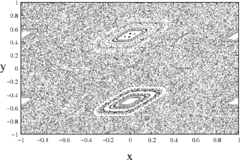
(b)

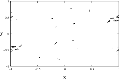
(c)

Figure 1: (a) The phase space plot of the standard map for $K=2.0$. (b) The plot for the corresponding embedding map for aerosols ($\alpha=0.8$, $\gamma=0.8$) and (c) bubbles ($\alpha=1.2$,$\gamma=0.4$). Random intial conditions distributed uniformly in the phase space were chosen.

We choose the standard map chirikov , to be our base map as it is a prototypical area-preserving system is widely studied in a variety of problems of both theoretical and experimental interest.

The standard map also serves as the usual test bed for the study of various transport phenomena and their quantifierswhite98 . The study of impurity dynamics using the standard map as the base flow, can thus give us a handle on the way in which these phenomena affect the impurity dynamics. Earlier studies of impurity dynamics using embeddings also use the standard map as the base map cart02 .

The parameter $K$ controls the chaoticity of the map. The chaoticity of the map is dependent on the initial condition and the map nonlinearity parameter $K$. The map equation is given by,

$${\bf x}_{n+1} = {\bf x}_{n}+{\bf y}_{n+1}\ ~{}~{}~{}~{}~{}~{}~{}~{}~{}~{}~{}(Mod\ 1)$$

$${\bf y}_{n+1} = {\bf y}_{n}+\frac{K}{2\pi}\sin(2\pi{\bf x}_{n})\ ~{}~{}(Mod\ 1)$$ (6)

This map is taken to be the base map ${\bf M(x}_{n})$ in Eq. (3). The phase space of this base standard map for $K=2.0$ is plotted in Fig. 1 in the region $x\in[-1,1],y\in[-1,1]$. The particle dynamics is governed by the 4 dimensional map ,

$$x_{n+1} = x_{n}+\frac{K}{2\pi}\sin(2\pi y_{n})+\delta_{n}^{x}$$

$$y_{n+1} = x_{n}+y_{n}+\frac{K}{2\pi}\sin(2\pi y_{n})+\delta_{n}^{y}$$

$$\delta_{n+1}^{x} = e^{-\gamma}[\alpha x_{n+1}-(x_{n+1}-\delta_{n}^{x})]$$

$$\delta_{n+1}^{y} = e^{-\gamma}[\alpha y_{n+1}-(y_{n+1}-\delta_{n}^{y})]$$ (7)

It is clear that this 4-dimensional map is invertible and dissipative. The embedding map has 3 parameters $K,\alpha,\gamma$. We plot the phase space portrait of the system evolved with random initial conditions at $K=2.0$, $\gamma=0.5$, and two values of $\alpha$, one in the aerosol regime $0<\alpha<1$ (Fig. 1(b)), and one in the bubble regime $1<\alpha<3$ (Fig. 1(c)). The phase space plot of the standard map at the same value of $K$ in Fig. 1(a) shows islands and chaotic regions separated by invariant tori which constitute barriers to transport. We observe from Figs. 1(b), and 1(c) that both the aerosols and bubbles have broken the barrier posed by the invariant curve and have targetted the islands forming structures. Thus, it is clear that the dissipation parameter $\gamma$ plays a vital role in the formation of structures. Therefore in order to identify the regimes in which clustering or mixing can take place, it is necessary to study the full phase diagram. The bifurcation diagram of the embedding map can also provide insights into the regimes that can be expected in the phase diagram.

(a)

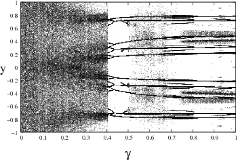
(b)

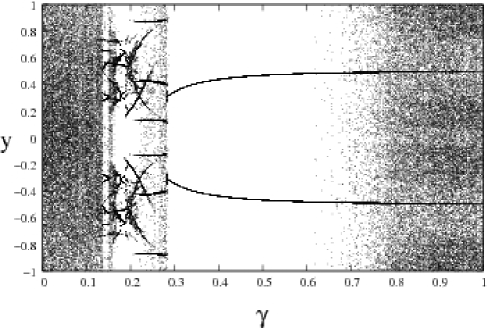
Figure 2: Typical bifurcation diagrams for the embedded standard map for $K=2.0$. a) aerosols ($\alpha=0.8$) b) bubbles ($\alpha=1.2$) for dissipation parameter ranging from $\gamma=0.0$ to $1.0$.

III The Bifurcation Diagram

We plot the bifurcation diagram of the embedded standard map (Fig. 2) for the parameter values $K=2.0$ and $\gamma$ values ranging from $0$ to $1$, and for two $\alpha$ values, $\alpha=0.8$ and $\alpha=1.2$ which correspond to the aerosol and bubble cases respectively. The bifurcation diagrams show many regions of periodic and chaotic behaviour for both the bubble and aerosol cases. This behaviour is reflected in the phase space plots of the map. The phase space plots for the aerosol case with $\gamma=0.8$, $\gamma=0.3$, and the bubble case with $\gamma=0.1$ can be seen in Fig. 3. Regimes with periodic orbits, structures and mixed regimes can clearly be seen here.

(c)

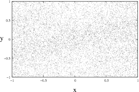
Figure 3: Phase space plots for fixed $K=2.0$ showing, (a) a chaotic structure in the phase space for the aerosol case $\alpha=0.9$, $\gamma=0.75$; (b) a chaotic structure in phase space for the bubble case $\alpha=1.05$, $\gamma=0.75$; (c) the mixing region in the bubble case $\alpha=1.7$, $\gamma=0.3$.

Thus the phase space plots show different types of dynamical behaviour depending on the $\gamma$ and $\alpha$ values. The phase diagram of the system in $\alpha-\gamma$ space is essential for identifying the parameter regimes where different kinds of dynamic behaviours can be seen.

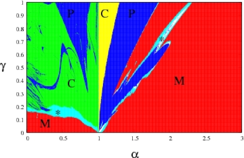
Figure 4: (Color Online) The phase diagram. The regimes with periodic structures are marked with P (blue). The regimes with chaotic structures are marked with C (green for aerosols and yellow for bubbles). The regimes with structures in a mixing background are marked with a ‘*’(light blue). The regimes with full mixing are marked with M (red).

IV The Phase Diagram

The phase diagram of the system can be constructed using the largest Lyapunov exponent as the characteriser and is shown in Fig. 4. For the calculation of the Lyapunov exponent, the first 5000 iterates are taken as transients and the next 1000 iterates are stored, for 100 random initial conditions, uniformly spread in the phase space.

The $\alpha$ values range from the aerosol regime $0\leq\alpha<1$, to the bubble regime $1<\alpha\leq 3$. Tongue-like structures are seen in the parameter space. Three types of regimes are seen in the phase diagram (i) regimes with periodic structures (P), where the largest Lyapunov exponent is negative, (ii) regimes with chaotic structures (C), (iii) mixing regimes (M), and (iv) chaotic structures in a mixing background. The Lyapunov exponent takes positive values in regimes (ii), (iii) and (iv). In the aerosol regime and the bubble regime, periodic orbits like those of Fig. 1(b) and (c) are seen inside the tongues marked by P (blue - (online)), and chaotic structures like those in Fig. 3(b) are seen in the regions marked by C (green -(online), in the aerosol regime and yellow - (online), in the bubble regime) of the phase diagram. The fully mixing regimes marked with M (red -(online), which exist in both aerosol and bubble regimes, are identified by the following procedure. At a given parameter value, the phase space is covered by a $100\times 100$ mesh, and the number of boxes accessed by the iterates is counted. The initial conditions and the transients are same as those that were used for calculating the Lyapunov exponent. The regions of parameter space where the iterates access more than $99\%$ of the phase space grid turn out to be fully mixing regions with no remanent of any chaotic structure seen in the phase space plot, and have been marked with an M.

(a)

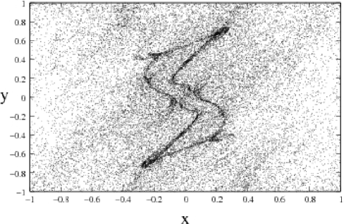
(b)

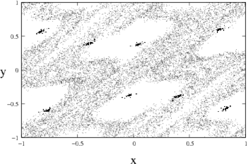
Figure 5: (a) A typical phase space plot for the regions with occupancy $<99\%$ and $>90\%$. Chaotic structures are seen in a mixing background. These regions are identified in the phase diagram - ‘*’ (light blue -online).(b) A typical phase space plot with occupancy $<90\%$ and $50\%~{}60\%$. They correspond to the unshaded (blank) regions in the phase diagram.

The regions where the iterates access $>90\%$ and $<99\%$ of the boxes in the phase space have been marked with an asterisk (*) (light blue-(online)). The phase space plots corresponding to this region have a chaotic structure in a well mixed background (Fig. 5(a)). The tiny patches of unshaded (blank) regions in the phase diagram are regions where $\lambda_{max}>0$ and the trajectories access less than $90\%$ of the grid in the phase space. Typically, the trajectories cover $50-60\%$ of the grid in the phase space in these regions. Fig. 5(b) shows a typical phase space plot for this case. Here, the iterates wander densely along the separatrices in the phase space, but large voids are seen in the phase space. However many iterates stick in the neighbourhood of the tiny dense structures seen in the middle of these voids.

V The Aerosol case: A crisis in the embedded standard map

The bifurcation diagram of the embedded standard map shows regimes where the attractor undergoes a sudden discontinuous change of type as the system parameter is varied. Such sudden discontinuous changes signal the onset of a crisis grebogi87 . The usual crises seen in dissipative dynamics are of the following types. In the attractor destruction type of crisis, a chaotic attractor is destroyed as the parameter passes through its critical crisis value. In the attractor widening or interior crisis, the size of the chaotic attractor increases suddenly. In the attractor merging crisis, two or more chaotic attractors merge to form one chaotic attractor. It is to be noted that the inverse of the above processes (i.e, the sudden creation, shrinking, or splitting of a chaotic attractor) occur as the parameter is varied in the other direction. In the case of our embedding map, the location and type of the crisis can be easily identified from the bifurcation diagram (see Fig. 2(b)).

(a)

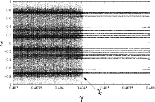
(b)

Figure 6: The identifiers of crisis: (a) the bifurcation diagram (b) the largest Lyapunov exponent plot, both obtained in the vicinity of the crisis, plotted as a function of the dissipation parameter $\gamma$ show a sudden change at the crisis where the dissipation parameter value $\gamma_{c}=0.40452$ .

The most prominent change in the size of the attractor is seen near $\gamma=0.40$. Here, as the parameter $\gamma$ decreases from 0.41 to 0.40 the attractor widens suddenly. The pre-crisis attractor has orbits of finite period, whereas after the crisis, the trajectories access the full range in $y$. The phase space plots at $\gamma=0.41$ and $\gamma=0.40$, corresponding to the pre-crisis and post-crisis situation respectively, are seen in Fig. 8. In the pre-crisis situation there are two period-10 attractors, and trajectories are confined to one or the other attractor, depending on the initial condition of the trajectory. After the crisis, the two attractors merge and widen into one. Thus we see the occurence of an attractor merging and widening crisis.

The exact parameter value at which the crisis occurs can be identified using standard quantifiers like the Lyapunov exponents, and also the bifurcation diagram.

(a)

(b)

Figure 7: The time series plots for a single trajectory for (a)the pre-crisis attractor, $\gamma=0.41$; (b) the post-crisis attractor, $\gamma=0.40$.

The close-up of the bifurcation diagram in Fig. 2(b) near $\gamma=0.40$ is shown in Fig. 6(a). As the dissipation parameter $\gamma$ is reduced from $\gamma=0.41$ through $\gamma=0.40$, a sudden widening is seen. The largest Lyapunov exponent, can also be used to identify the parameter value at crisis. Fig. 6(b) shows the Lyapunov exponent plotted in the vicinity of the crisis. The exponent clearly shows a sudden jump at $\gamma=0.40452$, which signifies the occurence of the crisis vishal . From the above identifiers, it is seen that, the critical parameter value at crisis is $\gamma_{c}=0.40452$ (to our numerical accuracy).

V.1 Crisis induced intermittency

We see the phenomenon of intermittency in the time series of the phase space co-ordinates in the neighbourhood of the attractor widening crisis. Let $\gamma_{c}$ be the parameter value where the attractor widening crisis occurs. In the pre-crisis region, ($\gamma>\gamma_{c}$), trajectories with arbitrary initial conditions in the phase space hop between the two attractors for small transient times. After this brief period, they settle into one of the attractors for arbitrarily long times (Fig. 7(a)).

In the post-crisis region, ($\gamma<\gamma_{c}$), trajectories starting from arbitrary initial conditions hop intermittently between the regions corresponding to the two pre-crisis attractors for arbitrarily long times and never settle into either of the attractors. The time interval between the hopping is random as can be seen from the Figure. 7(b). In the attractor merging and widening crisis, an orbit initially confined to only one of the pre-crisis attractors (Figure. 8(a)), say A or B, is able to access the widened single attractor composed of the two pre-crisis attractors A and B (Figure. 8(b)) after $\gamma$ is reduced to $\gamma_{c}$.

When a trajectory leaves the pre-crisis attractor and accesses the post-crisis attractor, a burst is said to have occurred. The trajectory settles back into the pre-crisis attractor after a time interval and a new burst is initiated after some time. The characteristic time for the orbit to stay in the pre-crisis attractor before a burst occurs is defined as $\tau$. For each value of $\gamma$ the distribution of the laminar lengths $\tau$ can thus be obtained. The average characteristic time $\tau$ in the neighborhood of the $\gamma_{c}$ was seen to follow a power law grebogi87 ,

$$\tau\sim(\gamma_{c}-\gamma)^{\beta}.$$ (8)

where the exponent was $\beta=-0.35$. Fig. 9 shows the log-log plot of $\tau$ vs $(\gamma_{c}-\gamma)$ which shows this scaling behaviour.

(a)

(b)

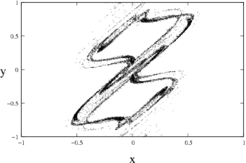
Figure 8: The phase space plots (a) the pre-crisis attractor with two period-10 orbits; $\gamma=0.41$ (b)the post-crisis attractor; $\gamma=0.40$.

We note that crisis induced intermittency is seen at several points on the left edge of the periodic tongue in the aerosol regime of the phase diagram. Power law scaling behaviour was seen at all these points. Unlike the aerosol case, no intermittency or crisis was observed anywhere in the bubble region.

The reason for this difference in behaviour of the aerosols and the bubbles may lie in the structure of the phase space. The invariant tori which act as barriers to transport in the neighbourhodd of elliptic fixed points break up at higher values of $K$ leaving behind leaky barriers or cantori. In the case of the motion of inertial partcles, the elliptic islands and their neighbourhoods act as centrifuges, by pushing away the heavier aerosols and entrapping the lighter bubbles bec07 . At high values of the dissipation $\gamma$ , the dissipation counteracts the effect of the centrifugal force on the aerosols, so that the they are trapped in the neighbourhood of the elliptic islands, despite the centrifugal force that pushes them out. However, at lower values of dissipation e.g. for our map, at $\gamma<\gamma_{c}$, where $\gamma_{c}$ is the criticalparameter at which crisis occurs, the centrifugal force pushes out the aerosols through the leaky barries leading to attractor widening and intermittency. In the case of the bubbles, both the dissipation and the centrifugal force work to trap the bubbles, and no crisis or intermittency is seen.

As mentioned above, the standard map which has been studied here is the prototypical area-preserving map. Hence, we expect that the key result, viz. that the dissipation of the fluid as well as the buoyancy of the particles affect the formation of coherent structures and the existence of mixing regions will apply to generic area preserving system. However, the details of the map, such as the existence of Cantori, and the size of the resonance zones will affect details like the existence of phenomena like crisis, crisis induced intermittency etc.

VI Conclusion

To summarize, the present work discusses the advection of passive scalars of finite size in an incompressible two-dimensional flow for situations where the particle density can differ from that of the fluid. The motion of the advected particles is represented by an embedding map with the area preserving standard map as the base map.

Figure 9: The log-log plot of the characteristic time $\tau$ versus $\gamma_{c}-\gamma$ with the slope $\beta=-0.35\pm 0.065087$.

The new embedded standard map is invertible and dissipative and contains three parameters, the nonlinearity $K$, the dissipation parameter $\gamma$ and the mass ratio parameter $\alpha$ which measures the extent to which the density of the particles differs from that of the fluid. The phase diagram of the system in the $\alpha-\gamma$ parameter space shows very rich structure. Three types of dynamical behaviours are seen periodic orbits, chaotic structures, and mixed regimes which can be partially or fully mixed. Periodic structures are seen inside tongues in the parameter space in the aerosol as well as bubble regimes. Thus, the clustering or preferential concentration of inertial particles can be seen in both the aerosol and bubble regimes. Chaotic structures can be seen outside the tongues in the aerosol regime. The bifurcation diagram indicates the existence of crises at parameter values on the edges of the tongues in this regime. The crisis is of the attractor merging and widening type in which two period ten orbits merge and widen into a chaotic attractor. Crisis induced intermittency is seen in the aerosol regime with charactersitic times $\tau$ which scale as $(\gamma_{c}-\gamma)^{\beta}$ where the exponent $\beta=-0.35$, and $\gamma_{c}$ is the critical value at which the crisis occurs. A well mixed regime is also seen for the aerosols. The bubble regime of the phase diagram shows periodic orbits, chaotic structures as well as partially and fully mixed regimes. No crisis or intermittency is seen here.

The obvious generalisation of our study is to the three dimensional case volume-preserving case. In this case, due to the presence of additional degrees of freedom, a much richer phase diagram is expected. While earlier studies show that regions which target tubular structures in phase space do existcartprl02 , the presence of additional stretching directions would perhaps indicate much richer structure and larger mixing regions in phase space. Detailed studies in this direction are in progress.

Our results have implications for the preferential concentration of inertial particles in flows, as well as for the targetting of periodic structures. Earlier results indicated that bubbles could breach elliptic islands and target structures, whereas aerosols could not. Our results indicate that the dissipation parameter $\gamma$ plays as crucial role in this as the density differential parameter $\alpha$, and the examination of the full phase diagram is necessary to draw conclusions about the parameter regimes where targetting and breaching can occur. We also see that mixing regimes can also exist, where random initial conditions can spread throughout the phase space. These results can have implications for the dynamics of impurities in diverse application contexts, e.g. that of the dispersion of pollutants in the atmosphere, flows with suspended microstructures, coagulation of material particles in flows and catalytic chemical reactions. We hope the present work will prove to be useful in some of these contexts.

VII acknowledgement

N.N.T thanks CSIR, India, for financial support. N.G thanks DST, India, for partial financial support under the project SP/S2/HEP/10/2003.

References

- (1) A.E. Motter, Y.C. Lai, and C. Grebogi, Phys. Rev. E 68, 056307(2003).
- (2) R. Reigada, F. Sagues,J.M. Sancho, Phys. Rev. E 64, 026307(2001).
- (3) A. Babiano, J.H.E. Cartwright, O. Piro, and A. Provenzale, Phys. Rev. Lett 84,5764 (2000).
- (4) J.H.E. Cartwright, M.O. Magnasco and O. Piro, Phys. Rev. E 65, 045203(R)(2002).
- (5) I.J. Benczik, Z. Toroczkai, and T. Tel, Phys. Rev. E 67, 036303 (2003).
- (6) R.D. Vilela, A.P.S. de Moura and C. Grebogi, Phys. Rev E 73, 026302(2006).
- (7) M.R.Maxey, J.J.Riley, Phys. Fluids 26, 883(1983).
- (8) M.R. Maxey, J. Fluid Mech, 174, 441(1987).
- (9) R.T. Pierrehumbert, Chaos 10, 61(2000).
- (10) D.R. Fereday, P.H. Haynes, and A. Wonhas , Phys. Rev. E 65, 035301(R)(2002).
- (11) J.H.E. Cartwright, M.O. Magnasco, O. Piro, I. Tuval, Phys. Rev. Lett 89, 264501(2002).
- (12) C. Grebogi, E. Ott, F. Romeiras, J. A. Yorke, Phys. Rev. A 36 , 5365(1987).
- (13) B.V.Chirikov, Phys. Rep 52,265 (1979).
- (14) R.B.White, S.Benkada, S.Kassibrakis and G.M. Zaslavsky, Chaos 8, 757 (1998).
- (15) V. Mehra and R. Ramaswamy, Phys. Rev E 53, 3420(1996).
- (16) J.Bec, L.Biferale, M.Cencini, A.Lanotte, S.Musacchio, F.Toschi, Phys. Rev. Lett 98, 084502 (2007).