The fluctuations, under time reversal, of the natural time and the entropy distinguish similar looking electric signals of different dynamics

Abstract

We show that the scale dependence of the fluctuations of the natural time itself under time reversal provides a useful tool for the discrimination of seismic electric signals (critical dynamics) from noises emitted from manmade sources as well as for the determination of the scaling exponent. We present recent data of electric signals detected at the Earth’s surface, which confirm that the value of the entropy in natural time as well as its value under time reversal are smaller than that of the entropy of a “uniform” distribution.

I Introduction

In a time series comprising $N$ events, the natural time $\chi_{k}=k/N$ serves as an indexVarotsos et al. (2001a, 2002a, 2002b) for the occurrence of the $k$-th event. In natural time analysis, the time evolution of the pair of the two quantities ($\chi_{k},Q_{k}$) is considered, where $Q_{k}$ denotes in general a quantity proportional to the energy released during the $k$-th event. In the case of dichotomous electric signals (e.g., seismic electric signal (SES) activities, i.e., low frequency $\leq 1$Hz electric signals that precede earthquakes, e.g., see Refs.Varotsos and Alexopoulos, 1986; Varotsos et al., 1986, 1988; Varotsos et al., 2003a, 2005a, 2001b; Varotsos et al., 1999; Sarlis et al., 1999; Varotsos et al., 1998; Varotsos, 2005) $Q_{k}$ stands for the duration of the $k$-th pulse (cf. The SES activities should not be confused with pulses of very short durations observed some minutes before earthquakesVarotsos et al. (2007a)). It has been shownAbe et al. (2005) that natural time domain is optimal for enhancing the signals’ localization in the time-frequency space, thus conforming to the desire to reduce uncertainty and extract signal information as much as possible. The entropy $S$ in natural time is definedVarotsos et al. (2003b) as the derivative with respect to $q$ of the fluctuation function $\langle\chi^{q}\rangle-\langle\chi\rangle^{q}$ at $q=1$:

$$S\equiv\langle\chi\ln\chi\rangle-\langle\chi\rangle\ln\langle\chi\rangle$$ (1)

where $\langle f(\chi)\rangle=\sum_{k=1}^{N}p_{k}f(\chi_{k})$ and $p_{k}=Q_{k}/\sum_{n=1}^{N}Q_{n}$. It is dynamic entropyVarotsos et al. (2004); Varotsos et al. (2005b) and exhibitsVarotsos et al. (2005c) concavity, positivity and LescheLesche (1982, 2004) stability. Note that $S$ should not be confused with $\text{Cov}[\chi,\ln\chi]\equiv\langle\chi\ln\chi\rangle-\langle\chi\rangle\langle\ln\chi\rangle$ since in general $\langle\ln\chi\rangle\neq\ln\langle\chi\rangle$. The value of the entropy upon considering the time reversal ${\cal T}$, i.e., ${\cal T}p_{k}=p_{N-k+1}$, is labelled by $S_{-}$. The value of $S_{-}$ isVarotsos et al. (2005c, 2006a, 2006b), in general, different from $S$, and thus $S$ does satisfy the conditions to be “causal” in the following sense (see Ref.Varotsos et al., 2005c and references therein): When studying a dynamical system evolving in time, the “causality” of an operator describing this evolution assures that the values assumed by the operator, at each time instant, depends solely on the past values of the system. Hence, a “causal” operator should be able to represent the evolution of the system according to the (true) time arrow, thus the operator can represent a real physical system evolving in time and reveal the differences arising upon time-reversal of the series.

The statistical properties of $S$ and $S_{-}$ have been studied in a variety of modelsVarotsos et al. (2006a, b). In the case of a “uniform” distribution $S=S_{-}=S_{u}(=\ln 2/2-1/4\approx 0.0966$). The “uniform” distribution (defined in Refs.Varotsos et al., 2001a, 2003c) has been analytically studied in Ref.Varotsos et al., 2004 and corresponds to the case when $Q_{k}$ are independent and identically distributed (IID) positive random variables of finite variance including the case of Markovian dichotomous electric signals studied in Ref.Varotsos et al., 2003b. The “uniform” distribution corresponds to $p(\chi)=1$, where $p(\chi)$ is a continuous probability density function (PDF) corresponding to the point probabilities $p_{k}$ used so far. When $Q_{k}$ of a “uniform” distribution are perturbed by a small linear trend, we findVarotsos et al. (2006a) (see also Eq.(4), below) that $(S-S_{u})(S_{-}-S_{u})<0$ (cf. this simple example, which shows that $S$ captures the effect of a linear trend, may be considered as clarifying the meaning of $S$, see Section V of Ref.Varotsos et al., 2006a). Another model studied is when the increments of $Q_{k}$ are positive IID, in this case we findVarotsos et al. (2006b) that $S\approx 0.048$ and $S_{-}\approx 0.088$ which are both smaller than $S_{u}$. The same holds, i.e., that both $S$ and $S_{-}$ are smaller than $S_{u}$, in the examples of an on-off intermittency model discussed in Ref.Varotsos et al., 2006a as well as for a multiplicative cascades modelVarotsos et al. (2006b) adjusted to describe turbulence data.

A case of practical importance is that of the SES activities. SES activities (critical dynamics) exhibit infinitely ranged long-range temporal correlationsVarotsos et al. (2003c, 2006a, 2006b) which are destroyedVarotsos et al. (2006b) after shuffling the durations $Q_{k}$ randomly. An interesting property emerged from the data analysis of several SES activities refers to the factVarotsos et al. (2006a) that both $S$ and $S_{-}$ values are smaller than the value of $S_{u}$, i.e.,

$$S,S_{-}<S_{u},$$ (2)

in addition to the fact that for SES activitiesVarotsos et al. (2001a, 2002b, 2002a) the variance

$$\kappa_{1}\equiv\langle\chi^{2}\rangle-\langle\chi\rangle^{2}\approx 0.070.$$ (3)

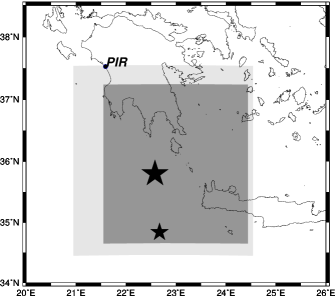
Figure 4: Map of the area surrounding the station PIR (solid dot) and the epicenters of the EQs (stars) with magnitude 5.2-units and 5.8-units that occurred on January 18 and February 3, 2007, respectively. The seismicity subsequent to the SES activities on November 14, 2006, has been studied in the gray shaded areas (the large and the small area are designated A and B, respectively).

These findings -which do not holdVarotsos et al. (2005c) for “artificial” noises (AN) (i.e., electric signals emitted from manmade sources)- have been supported by numerical simulations in fractional Brownian motion (fBm) time seriesVarotsos et al. (2006a, b) that have an exponent $\alpha_{DFA}$, resulted from the Detrended Fluctuation Analysis (DFA)Peng et al. (1994); Buldyrev et al. (1995), close to unity. This model have been applied since fBm (with a self-similarity index $H\approx 1$) has been foundWeron et al. (2005) as an appropriate type of modeling process for the SES activities. These simulations resulted in values of $S$ and $S_{-}$ that do obey relation (2) (see Fig.4 of Ref.Varotsos et al., 2006a) and $\kappa_{1}\approx 0.070$ (see Fig.3 of Ref.Varotsos et al., 2006b). It was then conjecturedVarotsos et al. (2006a) that the validity of the relation (2) stems from infinitely ranged long-range temporal correlations (cf. $H\approx 1$). On the other hand, for short-range temporal correlations (e.g. when modeling $Q_{k}$ by an autoregressive process $Q_{k}=aQ_{k-1}+g_{k}+c,|a|<1$ and $c$ stands for an appropriate constant to ensure positivity of $Q_{k}$ or $Q_{k}=|aQ_{k-1}+g_{k}|$ where $g_{k}$ is Gaussian IID variables) the values of both $S$ and $S_{-}$ approach (see Appendix A) that of $S_{u}$ and $\kappa_{1}\rightarrow\kappa_{u}$, where $\kappa_{u}=1/12$ denotes the corresponding value of the“uniform” distributionVarotsos et al. (2006b).

The scope of this paper is twofold: First, in Section II, we point out the usefulness of the study of the fluctuations of the natural time itself under time reversal. In particular, it enables the determination of the scaling exponent, thus allowing the distinction of SES activities from similar looking AN. Second, in Section III, we provide the most recent experimental data that strengthen the validity of the relations (2) and (3) for SES activities. The earthquakes that followed the latter SES activities are described in Section IV. Section V, summarizes our conclusions.

II The fluctuations of natural time under time reversal

The way through which the entropy in natural time captures the influence of the effect of a small linear trend has been studied, as mentioned, in Ref.Varotsos et al., 2006a on the basis of the parametric family of PDFs: $p(\chi;\epsilon)=1+\epsilon(\chi-1/2)$, where $\epsilon$ measures the extent of the linear trend. Such a family of PDFs shares the interesting property ${\cal T}p(\chi;\epsilon)=p(\chi;-\epsilon)$, i.e, the action of the time reversal is obtained by simply changing the sign of $\epsilon$. It has been shownVarotsos et al. (2006a) that the entropy $S(\epsilon)\equiv S[p(\chi;\epsilon)]$, as well as that of the entropy under time reversal $S_{-}(\epsilon)\equiv S[{\cal T}p(\chi;\epsilon)]$, $S_{-}(\epsilon)=S(-\epsilon)$, depend non-linearly on the trend parameter $\epsilon$:

$$S(\epsilon)=-\frac{1}{4}+\frac{\epsilon}{72}-\left(\frac{1}{2}+\frac{\epsilon}{12}\right)\ln\left(\frac{1}{2}+\frac{\epsilon}{12}\right).$$ (4)

However, it would be extremely useful to obtain a linear measure of $\epsilon$ in natural time. Actually, this is simply the average of the natural time itself:

$$\langle\chi\rangle=\int_{0}^{1}\chi p(\chi;\epsilon)d\chi=\frac{1}{2}+\frac{\epsilon}{12}.$$ (5)

If we consider the fluctuations of this simple measure upon time-reversal, we can obtain information on the long-range dependence of $Q_{k}$. We shall show that a measure of the long-range dependence emerges in natural time if we study the dependence of its fluctuations under time-reversal $\Delta\chi_{l}^{2}\equiv\text{E}[(\langle\chi\rangle-\langle{\cal T}\chi\rangle)^{2}]$ on the window length $l$ that is used for the calculation. Since ${\cal T}p_{k}=p_{l-k+1}$, we have

$$\Delta\chi_{l}^{2}\equiv\text{E}[(\langle\chi\rangle-{\langle\cal T}\chi\rangle)^{2}]=\text{E}\left\{\left[\sum_{k=1}^{l}\frac{k}{l}\left(p_{k}-p_{l-k+1}\right)\right]^{2}\right\},$$ (6)

where the symbol $\text{E}[\ldots]$ denotes the expectation value obtained when a window of length $l$ is sliding through the time series $Q_{k}$. $\text{E}[\ldots]$ is well defined when all the $\{p_{k}\}_{k=1,2,\dots l}$ involved in its argument are also well defined. The evaluation of $\text{E}[\ldots]$ can be carried out either by full or by Monte Carlo calculation. In order to achieve this goal, from the original time-series $\{Q_{k}\}_{k=1,2,\ldots L}$, we select segments $\{Q_{m_{0}+i-1}\}_{i=1,2,\ldots l}$ of length $l$, and the argument of $\text{E}[\ldots]$ is computed by substituting $p_{k}=Q_{m_{0}+k-1}/\sum_{i=1}^{l}Q_{m_{0}+i-1}$. The sum of the resulting values over the number of the selected segments (different $m_{0}$) is assigned to $\text{E}[\ldots]$. The full calculation refers to the case when $m_{0}$ takes all the $L-l+1(m_{0}=1,2,\ldots L-l+1)$ possible values, whereas the Monte Carlo when $m_{0}$ is selected randomly.

By expanding the square in the last part of Eq.(6), we obtain

$$\Delta\chi_{l}^{2}=\sum_{k=1}^{l}\left(\frac{k}{l}\right)^{2}\text{E}[(p_{k}-p_{l-k+1})^{2}]+\sum_{k\neq m}\frac{km}{l^{2}}\text{E}[(p_{k}-p_{l-k+1})(p_{m}-p_{l-m+1})].$$ (7)

The basic relationVarotsos et al. (2004) that interrelates $p_{k}$ is $\sum_{k=1}^{l}p_{k}=1$ or equivalently $p_{k}=1-\sum_{m\neq k}p_{m}$. By subtracting from the last expression its value for $k=l-k+1$, we obtain $p_{k}-p_{l-k+1}=-\sum_{m\neq k}(p_{m}-p_{l-m+1})$, and thus

$$(p_{k}-p_{l-k+1})^{2}=-\sum_{m\neq k}(p_{k}-p_{l-k+1})(p_{m}-p_{l-m+1}).$$ (8)

By substituting Eq.(8) into Eq.(7), we obtain

$$\Delta\chi_{l}^{2}=-\sum_{k=1}^{l}\left(\frac{k}{l}\right)^{2}\sum_{m\neq k}\text{E}[(p_{k}-p_{l-k+1})(p_{m}-p_{l-m+1})]+\sum_{k\neq m}\frac{km}{l^{2}}\text{E}[(p_{k}-p_{l-k+1})(p_{m}-p_{l-m+1})]$$ (9)

which simplifies to

$$\Delta\chi_{l}^{2}=-\sum_{k,m}\frac{(k-m)^{2}}{l^{2}}\text{E}[(p_{k}-p_{l-k+1})(p_{m}-p_{l-m+1})]$$ (10)

The negative sign appears because $(p_{k}-p_{l-k+1})$ and $(p_{m}-p_{l-m+1})$ are in general anti-correlated due to Eq.(8). Equation (10) implies that $\Delta\chi_{l}^{2}$ measures the long-range correlations in $Q_{k}$: If we assume that $-\text{E}[(p_{k}-p_{l-k+1})(p_{m}-p_{l-m+1})]\propto(k-m)^{2\chi_{H}}/l^{2}$ (cf. $p_{k}$ scales as $1/l$, e.g. see Varotsos et al. (2004)), we have that

$$\Delta\chi_{l}^{2}\propto l^{4+2\chi_{H}}/l^{4}$$ (11)

so that

$$\Delta\chi_{l}(\equiv\sqrt{\Delta\chi_{l}^{2}})\propto l^{\chi_{H}},$$ (12)

where $\chi_{H}$ is a scaling exponent.

II.1 Fractional Brownian motion and fractional Gaussian noise time series

In order to examine the validity of the above result Eq.(12) when $Q_{k}$ are coming from fBm or fractional Gaussian noise (fGn), we employed the following procedure: First, we generated fBm (or fGn) time-series $X_{k}$ (consisting of $2\times 10^{4}$ points) for a given value of $H$ using the Mandelbrot-Weierstrass functionMandelbrot and Wallis (1969); Szulga and Molz (2001); Frame et al. as described in Ref.Varotsos et al., 2006a. Second, since $Q_{k}$ should be positive, we normalized the resulting $X_{k}$ time-series to zero mean and unit standard deviation and then added to the normalized time-series $N_{k}$ a constant factor $c$ to ensure the positivity of $Q_{k}=N_{k}+c$ (for the purpose of the present study we used $c=10$). The resulting $Q_{k}$ time-series were then analyzed and the fluctuations of $\Delta\chi_{l}$ versus the scale $l$ are shown in Figs. 1(a) and 1(d) for fGn and fBm, respectively. The upper three panels of Fig.1 correspond to fGn while the lower three to fBm. We observe (see Fig.1(b)) that for fGn we have the interconnection: $\chi_{H}\approx H-1$ corresponding to descending curves(see Fig.1(a)), whereas for fBm the interconnection turns (see Fig.1(e)) to: $\chi_{H}\approx H$ corresponding to ascending curves(see Fig.1(d)).

In order to judge the merits or demerits of the procedure proposed here for the determination of the scaling exponent, we compare Figs.1(b) and 1(e) with Figs.1(c) and 1(f), respectively, that have been obtained by the well-established DFA methodPeng et al. (1994); Buldyrev et al. (1995). This comparison reveals that the results are more or less comparable for fGn, while for fBm the exponent $\chi_{H}$ deviates less from the behavior of an ideal estimator of the true scaling exponent (drawn in dashed green) compared to $\alpha_{DFA}$, especially for the largest $H$ values.

II.2 The fluctuations of the natural time to distinguish seismic electric signal activities from similar looking AN

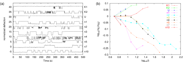
Figure 2: (color online) The log-log plot of $\Delta\chi_{l}$ versus the scale $l$ for three SES activities (K1, K2 and U) and seven AN (n1-n5, n7 and n10) treated in Ref.Varotsos et al., 2005c (cf. these signals have enough number of pulses in order to apply the present analysis). The values of $\Delta\chi_{l}$ are divided by the corresponding values $\Delta\chi_{5}$ at the scale $l=5$.

The physical meaning of the present analysis was further investigated by performing the same procedure in the time-series of the durations of those signals analyzed in Ref.Varotsos et al., 2005c that have enough number of pulses e.g.$\approx 10^{2}$ (cf. the signals depicted in Fig.3 could not be analyzed in view of the small number of pulses). The relevant results are shown in Fig.2. Their inspection interestingly indicates that all seven AN correspond to descending $\Delta\chi_{l}$ curves versus the scale $l$, while the three SES activities to ascending curves (in a similar fashion as in Figs.1(a) and 1(d), respectively) as expected from the fact that the latter exhibitVarotsos et al. (2003c) infinitely ranged long-ranged temporal correlations (having $H$ close to unity), while the former do not. Hence, the method proposed here enables the detection of long-range correlations even for datasets of small size ($\approx 10^{2}$), thus allowing the distinction of SES activities from AN.

III Recent data of Seismic Electric Signals activities

First, Fig.3(a) depicts an electric signal, consisting of a number of pulses, that has been recorded on November 14, 2006 at a station labelledEPA (a) PIR lying in western Greece (close to Pirgos city). This signal has been clearly collected at eleven measuring electric dipoles with electrodes installed at sites that are depicted in a map given in Ref.EPA, a. The signal is presented (continuous line in red) in Fig. 3(a) in normalized units, i.e., by subtracting the mean value and dividing by the standard deviation. For the reader’s convenience, the corresponding dichotomous representation is also drawn in Fig. 3(a) with a dotted (blue) line, while in Fig. 3(c) we show (in red crosses) how the signal is read in natural time. The computation of $S$ and $S_{-}$ leads to the following values: $S=0.070\pm 0.012$, $S_{-}=0.051\pm 0.010$. As for the variance $\kappa_{1}$, the resulting value is $\kappa_{1}=0.062\pm 0.010$. These values more or less obey the conditions (2) and (3) that have been found to hold for other SES activitiesVarotsos et al. (2006a). Note that the feature of this SES activity, it is similar to the one observed at the same station before the magnitude $M\approx 6.7$ earthquake that occurred on Jan 8, 2006, see Ref.Varotsos, 2006.

A closer inspection of Fig. 3(a) reveals the following experimental fact: An additional electric signal has been also detected (in the gray shaded area of Fig. 3(a)), which consists of pulses with markedly smaller amplitude than those of the SES activity discussed in the previous paragraph. This is reproduced (continuous line in red) in Fig. 3(b) in an expanded time scale and for the sake of the reader’s convenience its dichotomous representation is also marked by the dotted (blue) line, which leads to the natural time representation shown (dotted blue) in Fig. 3(c). The computation of $S$ and $S_{-}$ gives $S=0.077\pm 0.004$, $S_{-}=0.082\pm 0.004$, while $\kappa_{1}$ is found to be $\kappa_{1}=0.076\pm 0.005$. Hence, these values also obey the conditions (2) and (3) for the classification of this signal as an SES activity.

The two aforementioned signals have been followed by two significant earthquakes as described in Section IV. This conforms to their classification as SES activities, which has been completed in an early version of this paperVarotsos et al. (2006c) on November 16, 2006.

Second, very recently, i.e., on July 2, 2007 and July 10,2007, two separate electric signals were recorded at a station labelled PAT lying in central Greece (close to Patras city) at 38.32^oN21.90^oE. The signals are presented (continuous line in red) in Fig. 3 (d) and 3 (e) in normalized units in a similar fashion as in Figs.3(a),(b). Their corresponding dichotomous representation are also drawn with dotted (blue) lines, while in Fig.3(f) we show (in red crosses and blue asterisks, respectively) how the signals are read in natural time. The computation of $\kappa_{1}$, $S$ and $S_{-}$ leads to the following values: For the signal on July 2, 2007: $\kappa_{1}=0.072\pm 0.005$, $S=0.073\pm 0.007$, $S_{-}=0.081\pm 0.006$, for the signal on July 10, 2007: $\kappa_{1}=0.073\pm 0.004$, $S=0.085\pm 0.005$, $S_{-}=0.080\pm 0.004$. An inspection of these values reveals that they obey the conditions (2) and (3) and hence both signals can be classified as SES activities. The procedure for the current study of the subsequent seismicity that occurred after these SES activities is described in the next Section.

IV The seismic activity that followed the SES activities

We discriminate that during the last decade SES activities are publicized only when their amplitude indicates that the impending earthquake has an expectedVarotsos (2005); Varotsos et al. (2006b) magnitude comparable to 6.0 unit or larger.

IV.1 The case of the SES activities of Figs.3(a),(b)

According to the Athens observatory (the data of which will be used here), a strong earthquake (EQ) with magnitude 5.8-units occurred at 13:43 UT on February 3, 2007, with epicenter at $35.8^{o}$N $22.6^{o}$E, i.e., almost 80 km to the southwest of the 6.9 EQ of January 8, 2006, (cf. the magnitude announced from Athens observatory is equal to ML+0.5, where ML stands for the local magnitude). This was preceded by a 5.2-units EQ that occurred at 22:25 UT on January 18, 2007 at $34.8^{o}$N $22.7^{o}$E. The occurrence of these two EQs confirm the classification as SES activities of the signals depicted in Figs.3(a)and 3(b). (Note that preseismic information based on SES activities is issued only when the magnitude of the strongest EQ of the impending EQ activity is estimated -by means of the SES amplitudeEPA (b)- to be comparable to 6.0 units or largerVarotsos (2005).)

Here, we show that the occurrence times of the aforementioned two EQs can be estimated by following the procedure described in Refs.Varotsos et al., 2001a, 2005d, 2006a, 2006b and using the order parameter of seismicity proposed in Ref.Varotsos et al., 2005d, i.e, the normalized power spectrum in natural time $\Pi(\phi)$ as $\phi\rightarrow 0$ (see also below). We study how the seismicity evolved after the recording of the SES activities on November 14, 2006, at PIR station (which were classified as SES activities in the initially submitted version of the present paper on November 16, 2006). The study is made either in the area A:N${}_{34.45}^{37.54}$E${}_{20.95}^{24.54}$ or in the area B:N${}_{34.65}^{37.24}$E${}_{21.55}^{24.44}$ (see Fig.4), by considering three magnitude thresholds $M_{thres}=3.2$, 3.4 and 3.6 (hence six combinations were studied in total). If we set the natural time for seismicity zero at the initiation of the SES activity at 17:19 UT on November 14, 2006, we form time series of seismic eventsmag in natural time for various time windows as the number $N$ of consecutive (small) EQs increases. We then compute the normalized power spectrum Varotsos et al. (2001a, 2005d, 2006a, 2006b) in natural time $\Pi(\phi)$ for each of the time windows. Excerpts of these results, which refer to the values during the periods: (a) December 25, 2006, to January 17, 2007, and (b): January 18 to January 31, 2007 are depicted with red crosses in Fig.5, respectively. This figure corresponds to the small area B with $M_{thres}=3.4$. In the same figure, we plot in blue the normalized power spectrum obeying the relationVarotsos et al. (2001a, 2002a, 2002b, 2005d)

$$\Pi(\omega)=\frac{18}{5\omega^{2}}-\frac{6\cos\omega}{5\omega^{2}}-\frac{12\sin\omega}{5\omega^{3}}$$ (13)

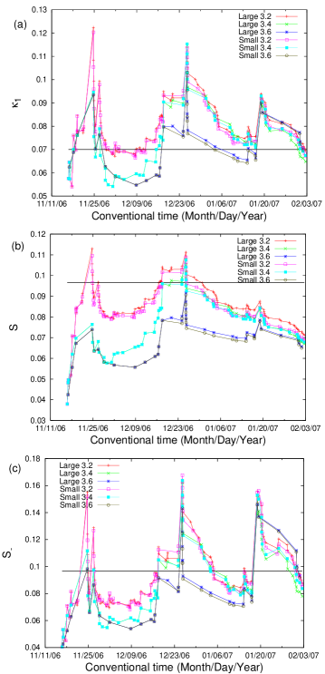
Figure 6: (color online) Evolution of the quantities $\kappa_{1}$, $S$ and $S_{-}$; they are shown in (a), (b) and (c), respectively, for three magnitude thresholds, i.e., $M\geq 3.2,3.4$ and $M\geq 3.6$, for both areas, i.e., the large (area A) and the small (area B). The solid horizontal lines correspond to $\kappa_{1}=0.07$ and $S_{u}=\ln 2/2-1/4$.

which holds when the system enters the critical stage ($\omega=2\pi\phi$, where $\phi$ stands for the natural frequencyVarotsos et al. (2001a, 2002a, 2002b); Varotsos (2005)). The date and the time of the occurrence of each small earthquake (with $M\geq 3.4$) that occurred in the area B, is written in green in each panel (see also Table 1). An inspection of Fig.5(a) reveals that the red line approaches the blue line as $N$ increases and a coincidence occurs at the small event of magnitude 3.7 that occurred at 03:22 UT on January 17, 2007, i.e., roughly two days before the 5.2-units EQ at 22:25 UT on January 18,2007. A similar behavior is observed in Fig.5(b) in which we see that a coincidence occurs at the small event of magnitude 3.6 at 18:40 UT on January 31, 2007, i.e., roughly three days before the strong EQ of magnitude 5.8-units that occurred at 13:43 UT on February 3, 2007. To ensure that these two coincidences in Figs.5(a) and (b) are true onesVarotsos et al. (2001a, 2005d, 2002b); Varotsos (2005); EPA (a) (see also below) we also calculate the evolution of the quantities $\kappa_{1}$,$S$ and $S_{-}$ and the results are depicted in Fig.6 for the three magnitude thresholds for each of the aforementioned two areas A and B.

The conditions for a coincidence to be considered as true are the following (e.g., see Ref.Varotsos et al., 2001a, see also Varotsos et al. (2005d, 2002b); Varotsos (2005); EPA (a)): First, the ‘average’ distance $\langle D\rangle$ between the empirical and the theoretical $\Pi(\phi)$(i.e., the red and the blue line, respectively, in Fig.5) should beVarotsos et al. (2001a, 2005d, 2002a); Varotsos (2005); EPA (a) smaller than or equal to $10^{-2}$. See Fig.7, where we plot $\langle D\rangle$ versus the conventional time during the whole period after the recording of the SES activities on November 14, 2006, for both areas, i.e., the large one (area A) and the small (area B) and the three magnitude thresholds. For the sake of the readers convenience, the mean value of the results obtained for the three thresholds is also shown in black. Second, in the examples observed to dateVarotsos et al. (2001a, 2005d, 2002b); Varotsos (2005); EPA (b, a), a few events before the coincidence leading to the strong EQ, the evolving $\Pi(\phi)$ has been found to approach that of Eq.(1), i.e., the blue one in Fig.5 , from below (cf. this reflects that during this approach the $\kappa_{1}$-value decreases as the number of events increases). In addition, both values $S$ and $S_{-}$ should be smaller than $S_{u}$ at the coincidence. Finally, since the process concerned is self-similar (critical dynamics), the time of the occurrence of the (true) coincidence should not change, in principle, upon changing either the (surrounding) area or the magnitude threshold used in the calculation. Note that in Fig.7, at the last small events ,i.e., the rightmost in Figs.5(a) and 5(b), respectively (i.e., the magnitude 3.7 event on January 17, 2007 and the second event of magnitude 3.6 on January 31, 2007) just before the occurrences of the 5.2-units and 5.8-units EQs, in both areas A and B, the mean value (see the black thick lines in Fig.7) of $\langle D\rangle$ obtained from the three magnitude thresholds become smaller than or equal to $10^{-2}$ . Hence, these two coincidences can be considered as true.

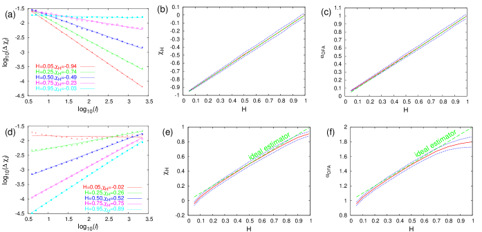
Figure 1: (color online) Examples of log-log plot of the fluctuations $\Delta\chi_{l}$ of the natural time under time reversal versus the scale $l$ for fGn (a) and fBm (d). (b) and (e) depict the values of the scaling exponent $\chi_{H}$, introduced here, versus the true exponent $H$ for fGn and fBm, respectively. For the sake of comparison, (c) and (f) are similar to (b) and (e), respectively, but for the DFA exponent $\alpha_{DFA}$. The (blue) dotted curves show the $\pm\sigma$ deviation from the average value (obtained after $10^{2}$ runs) depicted by the (red) solid curves. The (green) dashed straight lines correspond to the ideal behavior of each exponent and have been drawn as a guide to the eye.

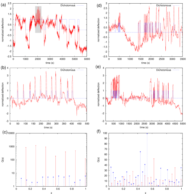
Figure 3: (color online) (a) The electric signal recorded on November 14, 2006 at PIR station (sampling rate $f_{exp}=1$Hz). The signal is presented here in normalized units (see the text). The corresponding dichotomous representation is shown with the dotted (blue) line. The gray shaded area shows an additional signal (consisting of pulses of smaller duration) superimposed on the previously mentioned signal. (b) The signal belonging to the gray shaded area in (a) is given here in an expanded time scale, while its dichotomous representation is marked by the dotted (blue) line. (c) How the signals in (a) and (b) are read in natural time: the continuous (red crosses) and dotted (blue asterisks) bars correspond to the durations of the dichotomous representations marked in (a) and (b), respectively.

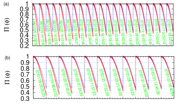
Figure 5: (color online) The normalized power spectrum(red) $\Pi(\phi)$ of the seismicity as it evolves event by event (whose date and time of occurrence are written in green in each panel) after the initiation of the SES activity on November 14, 2006. The two excerpts presented here, refer to the periods: (a) December 25, 2006, to January 17, 2007, and (b): January 18 to January 31, 2007, and correspond to the area B with $M_{thres}=3.4$. In each panel only the spectrum in the range $\phi\in[0,0.5]$ (for the reasons discussed in Refs.Varotsos et al., 2001a, 2005d) is depicted (separated by the vertical lines), whereas the $\Pi(\phi)$ of Eq.(13) is depicted by blue color. The minor horizontal ticks for $\phi$ are marked every 0.1.

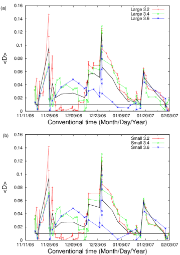
Figure 7: (color online)The average distance $\langle D\rangle$ between the calculated and the theoretical $\Pi(\phi)$ curves versus the conventional time. The calculation of $\langle D\rangle$ is made upon the occurrence of every consecutive earthquake when starting the calculation after the initiation of the SES activities on November 14, 2006 (depicted in Figs.3(a),(b)) for the large (area A) and the small (area B) for the three magnitude thresholds $M_{thres}=3.2$, 3.4 and 3.6. The black solid line corresponds to the mean value obtained from the three thresholds.

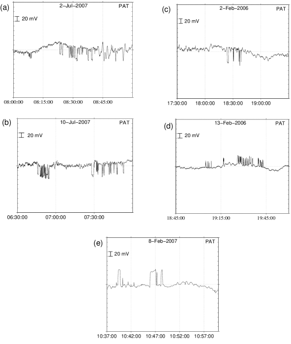
Figure 8: Recent SES activities recorded at PAT.

In summary, the SES activities recorded on November 14, 2006, at PIR station (presented in Figs.3(a),(b)) have been followed by two EQs with magnitudes 5.2-units and 5.8-units that occurred on January 18 and February 3, 2007. The time of the occurrences of these two EQs are determined within a narrow range of a few days upon analyzing, in natural time, the seismicity subsequent to the SES activities.

IV.2 The case of the SES activities of Figs.3(d),(e)

The actual amplitude (in mV) of the most recent SES activities recorded at PAT on July 2, 2007 and July 10, 2007 (see Fig.3(d) and (e), respectively) can be visualized in Figs.8(a) and 8(b) where the original recordings of a measuring electric dipole (with length $L\approx$5km) are reproduced. For the sake of comparison, in Figs.8(c),(d) we also present the corresponding SES activities at the same station, i.e., PAT, that precededVarotsos et al. (2006b); EPA (a) the magnitude 6.0-class earthquakes that occurred with epicenters at 37.6^oN20.9^oE on April 11 and 12,2006. Furthermore, in Fig.8(e), we show the SES activityVarotsos et al. (2007b) at PAT on February 8, 2007, which was followed by a magnitude class 6.0 earthquake at 38.3^oN20.4^oE that occurred on March 25, 2007.

In order to determine the occurrence time of the impending EQs, we currently apply the procedure explained in the previous subsection by studying the seismicity in the areas A, B, C (see Fig.9). Since the result should exhibit spatial scale invariance, the epicenter(s) will lie either in the area B or in C depending on whether the areas A and B or A and C show true coincidence.

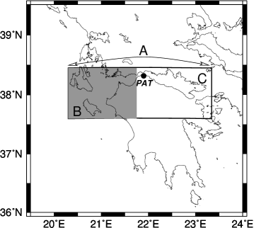
Figure 9: A map showing the areas A, B and C at which the analysis of the seismicity in natural time is currently carried out.

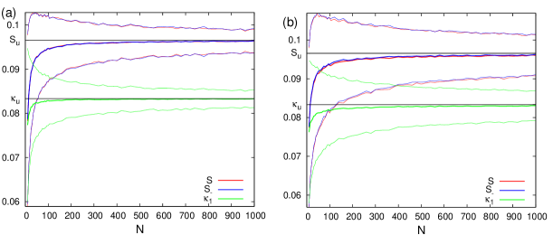
Figure 10: (color online) The thick colored lines in (a) and (b) depict the average value of $S$ (red),$S_{-}$ (blue) and $\kappa_{1}$ (green) versus the number of $Q_{k}$ for the two examples (i) and (ii), respectively, mentioned in the Appendix. The thinner colored lines refer to the $\pm\sigma$ deviation from the average value.

V Conclusions

First, the scale dependence of the fluctuations of the natural time under time reversal distinguish similar looking electric signals emitted from systems of different dynamics providing a useful tool for the determination of the scaling exponent. In particular, SES activities (critical dynamics) are distinguished from noises emitted from man-made electrical sources.

Second, recent data of SES activities are presented which confirm that the value of the entropy in natural time as well as its value under time reversal are smaller than that of a “uniform” distribution.

Appendix A The case of signals that exhibit short-range temporal correlations

Here, we present results of modeling $Q_{k}$ by short-ranged temporal correlated time-series. Two examples were treated by numerical simulation: (i) A stationary autoregressive process $Q_{k}=aQ_{k-1}+g_{k}+c$, $|a|<1$, where $g_{k}$ are Gaussian IID random variables, and $c$ stands for an appropriate constant to ensure positivity of $Q_{k}$. (ii) $Q_{k}=|aQ_{k-1}+g_{k}|$. Figure 10(a) depicts the results for $S$,$S_{-}$ and $\kappa_{1}$ for the first example versus the number of $Q_{k}$, whereas Fig.10(b) refers to the second example. In both cases $S$ and $S_{-}$ converge to $S_{u}$ whereas $\kappa_{1}$ to the value $\kappa_{u}=1/12$ corresponding to the “uniform” distribution. For the reader’s convenience, the values of $S_{u}$ and $\kappa_{u}$ are designated by the horizontal solid black lines.

Appendix B The seismic activity that followed the recent SES activities of Figs.8(a),(b)

Considering the Athens observatory preliminary catalogue, the seismic activity ($M_{thres}\geq 3.0$) that occurred in area A (see Fig.9) after the initiation of the SES activity on July 2, 2007 (Fig.8(a)) until 03:27 UT of September 25, 2007 is shown in Fig.11(a). The evolution of the corresponding parameters $\kappa_{1}$, $S$, $S_{-}$ and $\langle D\rangle$ calculated for three magnitude thresholds, i.e.,$M_{thres}=3.0,3.1$ and 3.2 are shown in Figs.11(b), (c) and (d) respectively. To investigate the spatial invariance, the computation was repeated for several smaller areas, three of which are shown in Figs.12,13 and 14 (which are different from the areas B and C of Fig.9) along with the evolution of the corresponding parameters. The same was repeated for an area (see Fig.15) somewhat larger than A. An inspection of all these figures, i.e., Figs.11 to15, suggests that presumably a true coincidence has just been approached, thus being very close to the critical point.

Appendix C The seismic activity that followed the most recent SES activities at PAT and PIR

Here, we report the update results of the seismic activity that followed the SES activity at PAT on October 9, 2008Varotsos et al. (2008) and the SES activity at PIR on December 12, 2008Varotsos et al. (2009) by following the procedure described by Sarlis et al.Sarlis et al. (2008). The subsequent seismicity of the former SES activity was studied in the area N${}_{37.5}^{38.6}$E${}_{19.8}^{23.3}$ while that of the latter in the selectivity map of PIR depicted in Fig. 16. The results, when considering the seismicity until early in the morning of February 2, 2009, for magnitude threshold M_thres=3.3, are shown in Figs. 17 and 18 for the former and the latter SES activities at PAT and PIR, respectively. An inspection of these figures reveals that in both areas the probability Prob($\kappa_{1}$) versus $\kappa_{1}$ -calculated in all the possible regions of each area as described in Ref.Sarlis et al. (2008)- maximizes at $\kappa_{1}\approx$ 0.070 upon the occurrence of the events marked with arrows, thus probably indicating the approach to the critical point.

Note added on February 20, 2009: Actually, at 23:16 UT on February 16, 2009 a strong earthquake with magnitude Ms(ATH)=6.0 (i.e., M_L(ATH)=5.5) occurred with an epicenter at 37.1^oN20.8^oE, which clearly lies inside the selectivity map of PIR depicted in Fig.16.

We now present the results, when considering the seismicity until early in the morning of February 19, 2009. Figure 19, depicts the results for M_thres=3.2 in the selectivity map of PAT (i.e., in the area N${}_{37.5}^{38.6}$E${}_{19.8}^{23.3}$), which show that the aforementioned probability Prob($\kappa_{1}$) versus $\kappa_{1}$ maximizes at $\kappa_{1}\approx$ 0.070 upon the occurrence of a M_L=3.2 event at 00:35 UT on February 19, 2009 with epicenter at 37.8^oN21.2^oE. As for the results in the selectivity map of PIR (i.e., the shaded area in Fig.16), they are shown in Fig.20 for M_thres=3.4 and reveal the following: After the aforementioned strong earthquake on February 16, 2009, the bimodal curve Prob($\kappa_{1}$) versus $\kappa_{1}$ shows a clear local maximum at $\kappa_{1}\approx$ 0.070 upon the occurrence of the M_L=3.5 event at 00:30 UT on February 18, 2009 with an epicenter at 34.9^oN23.4^oE. This local maximum does exhibit magnitude threshold invariance (since it also appears when investigating M_thres=3.3 and M_thres=3.5).

Updated note on March 13, 2009: Several hours before the occurrence of the aforementioned magnitude 6.0 earthquake on February 16, 2009, an electrical anomaly of significant amplitude, see Fig.21, appeared at PIR. It basically consists of three bay like transient changes, thus having a form essentially different than the SES activities that preceded the major earthquakes on February 14, 2008 and June 8, 2008. This electrical anomaly could be in principle attributed to the 6.0 earthquake on February 16, 2009 that occurred almost 11 hours later, but this earthquake was also preceded by the SES activity at PIR on December 12, 2008. Alternatively, this anomaly might be related to a new impending earthquake. For this reason, a natural time analysis of the seismicity subsequent to the electrical anomaly of February 16, 2009 was carried out. In this calculation we considered the events that occurred in the PIR selectivity map shown in Fig.22 (cf. this, which is slightly different than that depicted in Fig.16, has been drawn by taking into account the whole region to the west of the Hellenides). The results of the analysis shown in Fig.23 indicate that for M_thres=3.6 and 3.5 (see a and b, respectively) the probability Prob($\kappa_{1}$) maximizes at $\kappa_{1}\approx$ 0.070 upon the occurrence of a M_L=3.6 event at 02:48 UT on March 9, 2009, while for M_thres=3.3 the maximization occurs upon the occurrence of a M_L=3.3 event on March 10, 2009. Interestingly, a similar analysis (subsequent to the SES activity at PAT) in the selectivity map of PAT, i.e., in the area N${}_{37.5}^{38.6}$E${}_{19.8}^{23.3}$, reveals that a maximization of Prob($\kappa_{1}$) at $\kappa_{1}\approx$ 0.070 also occurs on March 10, 2009 (see Fig.24). We are currently investigating the spatial and magnitude threshold invariance of the aforementioned maxima to examine whether they actually point to an approach to the critical point.

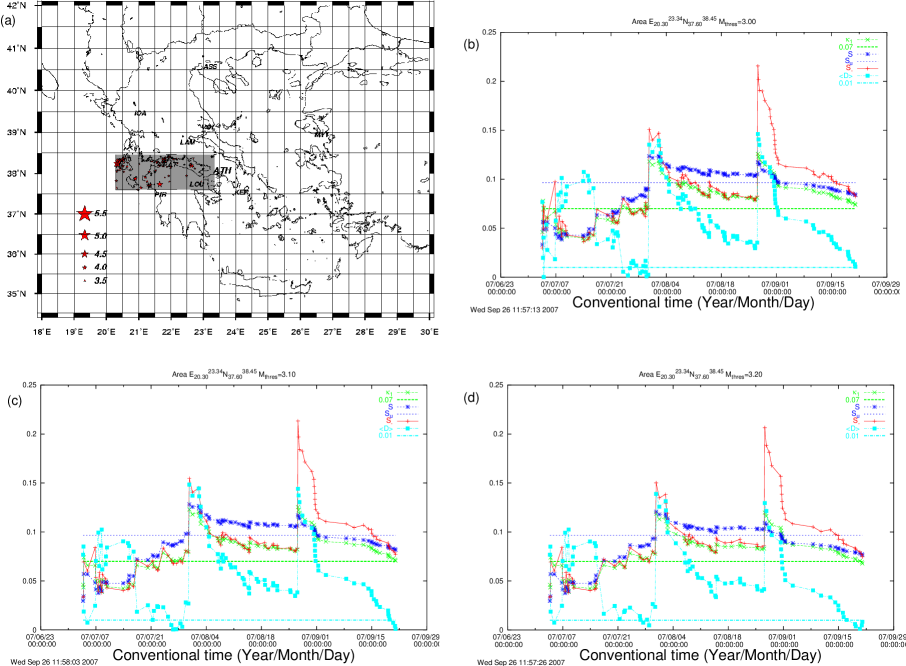
Figure 11: (color online) Results of the analysis of seismicity in the dark gray shaded area of (a) after the SES initiation on July 2, 2007.

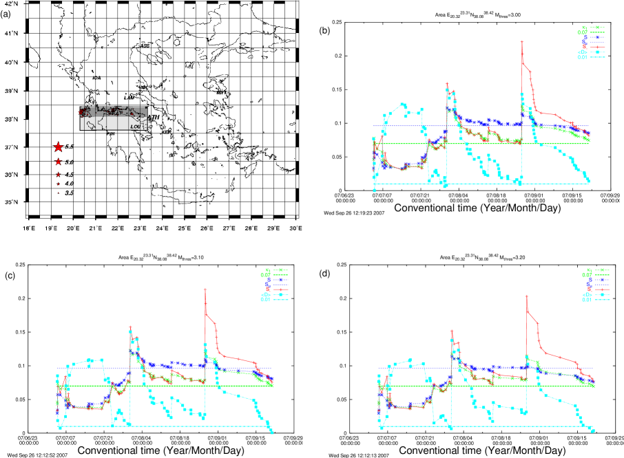
Figure 12: (color online) Results of the analysis of seismicity in the dark gray shaded area of (a) after the SES initiation on July 2, 2007.

Figure 13: (color online) Results of the analysis of seismicity in the dark gray shaded area of (a) after the SES initiation on July 2, 2007.

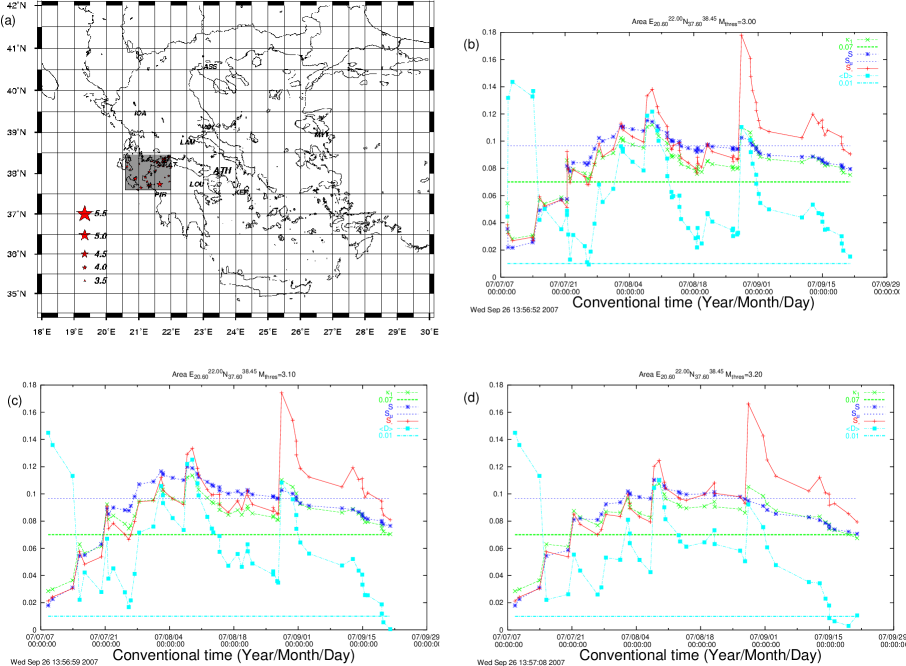
Figure 14: (color online) Results of the analysis of seismicity in the dark gray shaded area of (a) after the SES initiation on July 2, 2007.

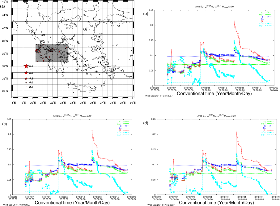
Figure 15: (color online) Results of the analysis of seismicity in the dark gray shaded area of (a) after the SES initiation on July 2, 2007.

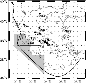
Figure 16: The selectivity map of PIR (shaded area) along with the selectivity map of PAT (rectangular area)

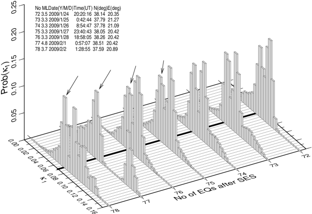
Figure 17: The Prob($\kappa_{1}$) versus $\kappa_{1}$ of the seismicity for M_thres=3.3 subsequent to the SES activity recorded at PAT on October 9, 2008 within the selectivity map of PAT shown in Fig. 16. For the sake of clarity, only the last 7 events are depicted. The arrows mark the maxima at $\kappa_{1}$=0.070 (see the text)

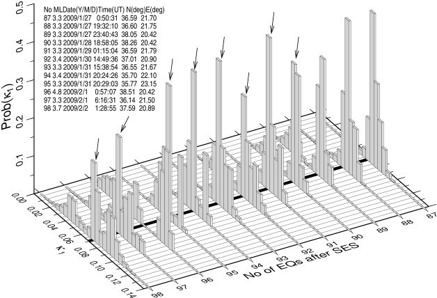
Figure 18: The Prob($\kappa_{1}$) versus $\kappa_{1}$ of the seismicity for M_thres=3.3 subsequent to the SES activity recorded at PIR on December 12, 2008 within the selectivity map of PIR shown in Fig. 16. For the sake of clarity, only the last 12 events are depicted. The arrows mark the maxima at $\kappa_{1}$=0.070 (see the text).

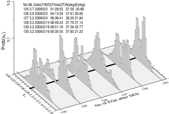
Figure 19: Prob($\kappa_{1}$) versus $\kappa_{1}$ of the seismicity for M_thres=3.2 subsequent to the SES activity recorded at PAT on October 9, 2008 within the area N${}_{37.5}^{38.6}$E${}_{19.8}^{23.3}$. For the sake of clarity, only the last 6 events are depicted. Prob($\kappa_{1}$) exhibits a maximum at $\kappa_{1}$=0.070 upon the occurrence of the 3.2 event on February 19, 2009 (see the text).

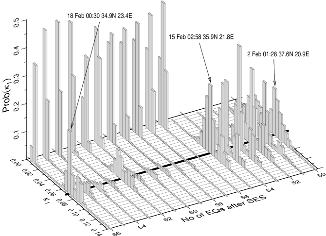
Figure 20: Prob($\kappa_{1}$) versus $\kappa_{1}$ of the seismicity for M_thres=3.4 subsequent to the SES activity recorded at PIR on December 12, 2008 within the selectivity map of PIR shown in Fig. 16. For the sake of clarity, only the last 17 events are depicted. The arrows mark the maxima of Prob($\kappa_{1}$) at $\kappa_{1}$=0.070 (see the text).

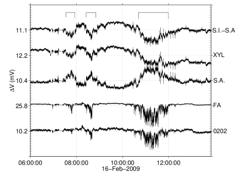
Figure 21: Electrical recordings from PIR; for the sites of the electrodes see Ref.EPA (a).

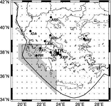
Figure 22: The selectivity map of PIR when including the whole region to the west of Hellenides (shaded area). The rectangular area corresponds to the selectivity map of PAT.

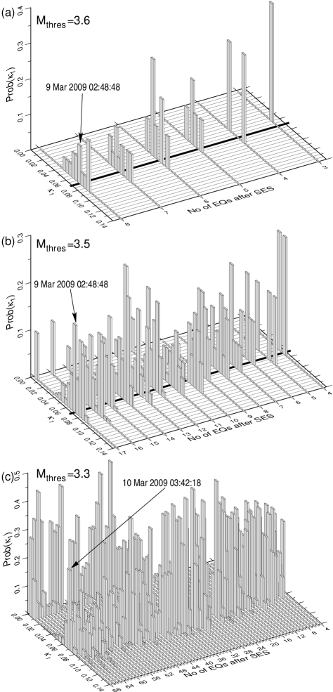
Figure 23: Prob($\kappa_{1}$) versus $\kappa_{1}$ of the seismicity in the shaded region of Fig.22 for M_thres=3.6 (a), 3.5 (b) and 3.3 (c) subsequent to the electrical anomaly shown in Fig.21. The arrows mark the maxima of Prob($\kappa_{1}$) at $\kappa_{1}$=0.070 (see the text).

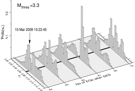
Figure 24: Prob($\kappa_{1}$) versus $\kappa_{1}$ of the seismicity for M_thres=3.3 subsequent to the SES activity recorded at PAT on October 9, 2008 within the area N${}_{37.5}^{38.6}$E${}_{19.8}^{23.3}$. For the sake of clarity, only the last 6 events are depicted. Prob($\kappa_{1}$) exhibits a maximum at $\kappa_{1}$=0.070 upon the occurrence of the event at 15:22 UT on March 10, 2009.

Table 1: The catalogue ($M_{thres}=3.2$) of the Institute of Geodynamics of the National Observatory of Athens (GI-NOA) (available from http://www.gein.noa.gr/services/monthly-list.html on February 5, 2007) for the Large area (area A) during the following period: From the initiation of the SES activity almost at 17:00 UT on November 14, 2006 (Fig.1 of the main text) until the occurrence of the 5.8-units earthquake on February 3, 2007. Note that Ms(ATH)=M+0.5, where M stands for the local magnitude ML or the “duration” magnitude MD. Two events reported by GI-NOA: at 17:32:23.7 on January 28, 2007, and at 5:11:06.5 on January 30, 2007, were omitted since they could not be independently confirmed by other seismic networks operating at that time.

$N$	Year	Month	Day	UT	Lat.(oN)	Lon.(oE)	depth(km)	M
1	2006	11	16	4:20:40.0	35.66	23.26	54	3.5
2	2006	11	16	12:30:50.3	35.44	23.42	5	3.7
3	2006	11	16	18:50:02.5	36.97	23.11	25	3.7
4	2006	11	16	21:53:12.5	35.72	24.33	10	3.4
5	2006	11	17	16:31:26.4	36.69	23.32	24	3.2
6	2006	11	18	3:48:58.3	34.79	24.07	16	3.6
7	2006	11	18	21:51:21.8	34.78	24.36	34	3.2
8	2006	11	19	9:31:09.1	35.73	21.95	19	3.6
9	2006	11	19	10:54:52.3	35.99	23.65	10	3.2
10	2006	11	19	14:11:45.4	35.75	22.55	24	3.3
11	2006	11	21	5:57:05.5	34.81	24.28	54	3.3
12	2006	11	21	8:42:06.0	37.42	21.96	19	3.2
13	2006	11	21	12:50:34.0	35.45	23.90	10	3.3
14	2006	11	24	17:16:58.4	37.16	21.58	12	4.1
15	2006	11	24	17:42:56.3	35.60	23.50	7	3.3
16	2006	11	24	20:26:02.9	37.12	21.56	11	3.5
17	2006	11	24	21:41:44.1	37.21	21.63	8	3.3
18	2006	11	25	3:14:31.2	34.94	23.91	5	3.2
19	2006	11	25	4:55:01.3	37.15	21.86	9	3.3
20	2006	11	25	9:30:18.1	36.75	21.73	12	3.6
21	2006	11	26	17:58:05.5	35.45	23.30	11	4.1
22	2006	11	26	19:45:54.7	35.40	23.27	2	3.3
23	2006	11	26	23:57:49.1	35.47	23.36	5	3.4
24	2006	11	27	3:12:49.8	35.42	23.31	9	3.3
25	2006	11	27	11:58:03.7	35.53	23.43	24	3.2
26	2006	11	28	9:07:38.6	36.07	22.35	10	3.3
27	2006	11	28	15:07:43.1	36.06	22.42	43	3.6
28	2006	11	28	15:42:59.4	35.71	22.11	10	3.4
29	2006	11	28	22:54:24.0	37.06	21.51	12	3.2
30	2006	11	29	14:11:02.8	35.97	23.11	19	3.5
31	2006	11	30	23:30:58.6	35.43	23.32	3	3.2
32	2006	12	1	2:37:02.1	35.58	23.60	10	3.5

Table 1: Continued

$N$	Year	Month	Day	UT	Lat.(oN)	Lon.(oE)	depth(km)	M
33	2006	12	1	19:57:55.4	37.07	21.47	3	3.2
34	2006	12	1	22:49:35.6	35.72	22.52	114	3.7
35	2006	12	2	0:29:20.8	34.74	22.87	45	3.2
36	2006	12	2	10:30:35.3	37.42	22.04	4	3.3
37	2006	12	3	1:53:22.4	36.72	21.81	24	3.5
38	2006	12	3	2:37:36.7	36.40	21.66	10	3.2
39	2006	12	4	19:32:24.0	34.99	23.44	14	3.4
40	2006	12	7	22:22:49.4	35.73	23.17	32	3.2
41	2006	12	8	10:54:40.0	34.95	23.42	5	3.3
42	2006	12	8	12:48:15.5	37.02	21.93	10	3.2
43	2006	12	8	19:57:27.2	35.06	23.50	7	3.6
44	2006	12	9	22:45:56.5	35.89	23.38	24	3.4
45	2006	12	10	3:29:46.1	34.84	24.48	10	3.2
46	2006	12	10	12:41:27.6	35.80	23.04	59	3.2
47	2006	12	11	3:36:22.0	35.74	24.08	16	3.4
48	2006	12	11	19:11:29.4	35.93	23.40	15	3.2
49	2006	12	12	3:40:55.0	35.54	22.81	17	3.7
50	2006	12	13	9:45:40.0	37.25	21.94	20	3.2
51	2006	12	14	16:44:02.0	35.95	23.46	10	3.3
52	2006	12	15	4:40:12.5	35.01	23.37	80	3.4
53	2006	12	15	10:23:32.1	36.09	22.25	45	3.7
54	2006	12	16	10:43:15.4	34.85	24.33	6	3.6
55	2006	12	16	15:23:33.2	34.92	23.45	5	3.7
56	2006	12	17	4:44:38.7	34.73	24.00	30	3.5
57	2006	12	17	4:44:42.7	35.15	24.12	59	3.5
58	2006	12	17	10:20:49.7	36.06	21.76	37	3.3
59	2006	12	17	14:13:23.4	36.21	21.70	10	3.4
60	2006	12	17	20: 0:20.6	34.84	24.21	34	4.0
61	2006	12	17	22:38:37.5	36.65	21.00	10	3.2
62	2006	12	20	4:34:09.2	37.48	21.50	10	3.2
63	2006	12	20	4:45:15.0	35.42	21.43	10	3.5
64	2006	12	20	19:27:32.5	34.60	23.79	11	3.8
65	2006	12	20	20:17:02.7	36.68	21.50	4	3.2
66	2006	12	24	6:58:02.3	34.94	24.03	10	3.6
67	2006	12	24	7:12:11.4	36.29	22.20	24	3.8
68	2006	12	25	14:08:59.4	34.83	22.66	39	4.4
69	2006	12	25	14:15:50.1	34.99	23.04	39	4.0
70	2006	12	25	14:18:50.7	35.09	23.06	27	4.0
71	2006	12	25	14:22:30.3	35.01	22.95	18	3.9
72	2006	12	25	14:57:00.5	35.04	22.84	14	4.1
73	2006	12	25	17:29:17.9	35.92	23.62	5	3.2
74	2006	12	25	18:13:44.5	35.09	23.29	10	3.7
75	2006	12	28	6:32:19.4	37.53	21.81	10	3.2
76	2006	12	29	2:00:54.9	36.77	21.81	5	3.3
77	2006	12	30	22:51:38.0	35.39	23.34	13	3.2

Table 1: Continued

$N$	Year	Month	Day	UT	Lat.(oN)	Lon.(oE)	depth(km)	M
78	2006	12	31	7:00:51.9	35.85	22.08	10	3.2
79	2006	12	31	18: 6:27.5	35.14	22.76	12	3.7
80	2007	1	1	15:27:48.7	34.72	24.12	23	3.5
81	2007	1	3	15:04:04.9	35.37	23.29	10	3.4
82	2007	1	3	18:18:34.5	36.54	21.74	26	3.8
83	2007	1	4	7:57:08.3	37.37	21.56	15	3.3
84	2007	1	4	14:55:24.6	36.29	21.92	10	3.2
85	2007	1	4	17:42:54.7	34.91	23.61	45	3.3
86	2007	1	4	20:41:40.9	34.89	24.13	48	3.2
87	2007	1	4	22:47:39.1	36.96	21.07	25	3.2
88	2007	1	7	14:07:11.5	37.10	21.93	26	3.2
89	2007	1	8	16:13:02.8	35.10	23.03	10	3.4
90	2007	1	9	9:55:29.2	36.70	21.55	31	3.4
91	2007	1	9	15:54:47.3	35.89	23.61	3	3.2
92	2007	1	9	23:09:20.0	36.21	22.70	116	3.6
93	2007	1	11	5:50:39.5	35.02	22.48	38	3.8
94	2007	1	13	11:12:43.3	35.48	23.51	8	3.4
95	2007	1	14	9:09:23.0	35.30	23.38	3	3.8
96	2007	1	14	16:43:01.6	35.06	23.20	85	4.1
97	2007	1	15	0:55:18.8	37.47	21.07	15	3.2
98	2007	1	15	3:13:45.8	36.06	22.40	13	3.4
99	2007	1	15	6:56:47.0	35.42	23.56	33	3.3
100	2007	1	15	17:50:48.7	36.56	21.65	5	3.4
101	2007	1	17	1:52:18.8	36.20	21.58	34	3.7
102	2007	1	17	3:22:53.9	35.34	23.53	12	3.7
103	2007	1	18	22:25:23.0	34.84	22.67	39	4.7
104	2007	1	18	23:31:32.7	34.76	21.36	10	3.4
105	2007	1	19	8:42:22.8	34.72	22.57	38	4.4
106	2007	1	20	7:05:37.0	34.95	24.09	19	3.5
107	2007	1	20	7:24:24.6	34.86	23.96	19	3.4
108	2007	1	20	10:24:55.4	36.88	22.10	10	3.2
109	2007	1	20	11:57:23.7	36.69	22.47	10	3.5
110	2007	1	20	23:50:04.1	34.93	24.40	28	3.3
111	2007	1	21	17:52:34.9	35.46	23.46	11	3.4
112	2007	1	25	10:24:47.3	35.33	23.40	2	3.3
113	2007	1	25	21:09:45.7	35.09	23.25	22	4.3
114	2007	1	28	15:19:23.6	36.29	23.17	25	3.4
115	2007	1	28	19:12:16.4	36.95	21.13	10	3.4
116	2007	1	30	5:11:08.9	35.94	23.41	28	3.3
117	2007	1	30	10:38:42.7	36.98	21.10	12	3.5
118	2007	1	30	21:11:43.0	36.13	22.17	30	3.3
119	2007	1	31	4:56:59.1	35.49	22.78	36	3.4
120	2007	1	31	14:45:09.7	34.67	22.42	29	3.6
121	2007	1	31	18:40:54.1	36.26	22.48	23	3.6
122	2007	2	1	16:45:35.3	34.69	22.46	21	3.9
123	2007	2	1	21:06:54.7	36.06	21.62	42	3.2
124	2007	2	2	6:39:05.6	35.21	23.25	33	3.3
125	2007	2	2	13:27:53.1	37.22	21.63	4	3.4

References

- Varotsos et al. (2001a) P. A. Varotsos, N. V. Sarlis, and E. S. Skordas, Practica of Athens Academy 76, 294 (2001a).
- Varotsos et al. (2002a) P. A. Varotsos, N. V. Sarlis, and E. S. Skordas, Phys. Rev. E 66, 011902 (2002a).
- Varotsos et al. (2002b) P. Varotsos, N. Sarlis, and E. Skordas, Acta Geophys. Pol. 50, 337 (2002b).
- Varotsos and Alexopoulos (1986) P. Varotsos and K. Alexopoulos, Thermodynamics of Point Defects and their Relation with Bulk Properties (North Holland, Amsterdam, 1986).
- Varotsos et al. (1986) P. Varotsos, K. Alexopoulos, K. Nomicos, and M. Lazaridou, Nature (London) 322, 120 (1986).
- Varotsos et al. (1988) P. Varotsos, K. Alexopoulos, K. Nomicos, and M. Lazaridou, Tectonophysics 152, 193 (1988).
- Varotsos et al. (2003a) P. Varotsos, N. Sarlis, and E. Skordas, Phys. Rev. Lett. 91, 148501 (2003a).
- Varotsos et al. (2005a) P. Varotsos, N. Sarlis, and E. Skordas, Appl. Phys. Lett. 86, 194101 (2005a).
- Varotsos et al. (2001b) P. Varotsos, N. Sarlis, and E. Skordas, Proc. Jpn. Acad. Ser. B 77, 93 (2001b).
- Varotsos et al. (1999) P. Varotsos, N. Sarlis, and M. Lazaridou, Phys. Rev. B 59, 24 (1999).
- Sarlis et al. (1999) N. Sarlis, M. Lazaridou, P. Kapiris, and P. Varotsos, Geophys. Res. Lett. 26, 3245 (1999).
- Varotsos et al. (1998) P. Varotsos, N. Sarlis, M. Lazaridou, and P. Kapiris, J. Appl. Phys. 83, 60 (1998).
- Varotsos (2005) P. Varotsos, The Physics of Seismic Electric Signals (TERRAPUB, Tokyo, 2005).
- Varotsos et al. (2007a) P. Varotsos, N. Sarlis, E. Skordas, and M. Lazaridou, Appl. Phys. Lett. 90, 064104 (2007a).
- Abe et al. (2005) S. Abe, N. V. Sarlis, E. S. Skordas, H. K. Tanaka, and P. A. Varotsos, Phys. Rev. Lett. 94, 170601 (2005).
- Varotsos et al. (2003b) P. A. Varotsos, N. V. Sarlis, and E. S. Skordas, Phys. Rev. E 68, 031106 (2003b).
- Varotsos et al. (2004) P. A. Varotsos, N. V. Sarlis, E. S. Skordas, and M. S. Lazaridou, Phys. Rev. E 70, 011106 (2004).
- Varotsos et al. (2005b) P. A. Varotsos, N. V. Sarlis, E. S. Skordas, and M. S. Lazaridou, Phys. Rev. E 71, 011110 (2005b).
- Varotsos et al. (2005c) P. A. Varotsos, N. V. Sarlis, H. K. Tanaka, and E. S. Skordas, Phys. Rev. E 71, 032102 (2005c).
- Lesche (1982) B. Lesche, J. Stat. Phys. 27, 419 (1982).
- Lesche (2004) B. Lesche, Phys. Rev. E 70, 017102 (2004).
- Varotsos et al. (2006a) P. A. Varotsos, N. V. Sarlis, E. S. Skordas, H. K. Tanaka, and M. S. Lazaridou, Phys. Rev. E 73, 031114 (2006a).
- Varotsos et al. (2006b) P. A. Varotsos, N. V. Sarlis, E. S. Skordas, H. K. Tanaka, and M. S. Lazaridou, Phys. Rev. E 74, 021123 (2006b).
- Varotsos et al. (2003c) P. A. Varotsos, N. V. Sarlis, and E. S. Skordas, Phys. Rev. E 67, 021109 (2003c).
- Peng et al. (1994) C.-K. Peng, S. V. Buldyrev, S. Havlin, M. Simons, H. E. Stanley, and A. L. Goldberger, Phys. Rev. E 49, 1685 (1994).
- Buldyrev et al. (1995) S. V. Buldyrev, A. L. Goldberger, S. Havlin, R. N. Mantegna, M. E. Matsa, C.-K. Peng, M. Simons, and H. E. Stanley, Phys. Rev. E 51, 5084 (1995).
- Weron et al. (2005) A. Weron, K. Burnecki, S. Mercik, and K. Weron, Phys. Rev. E 71, 016113 (2005).
- Mandelbrot and Wallis (1969) B. Mandelbrot and J. R. Wallis, Water Resources Research 5, 243 (1969).
- Szulga and Molz (2001) J. Szulga and F. Molz, J. Stat. Phys. 104, 1317 (2001).
- (30) M. Frame, B. Mandelbrot, and N. Neger, fractal Geometry, Yale University, available from http://classes.yale.edu/fractals/, see http://classes.yale.edu/Fractals/RandFrac/fBm/fBm4.html.
- EPA (a) eprint See EPAPS document No. E-PLEEE8-74-190608 for additional information, originally from P. Varotsos, N. Sarlis, E. Skordas, H. Tanaka, and M. Lazaridou, Phys. Rev. E 74, 021123 (2006). For more information on EPAPS, see http:// www.aip.org/pubservs/epaps.html.
- Varotsos (2006) P. A. Varotsos, Proc. Japan Acad., Ser. B 82, 86 (2006).
- Varotsos et al. (2006c) P. Varotsos, N. Sarlis, E. Skordas, and M. Lazaridou (2006c), arXiv:cond-mat/0611437v1 [cond-mat.stat-mech].
- EPA (b) eprint The time of the impending earthquake can be determined by means of the procedure described in EPAPS Document No. E-PLEEE8-73-134603 for additional information, originally from P.A. Varotsos, N.V. Sarlis, E.S. Skordas, H.K. Tanaka and M.S. Lazaridou, Phys. Rev. E 73, 031114 (2006). For more information on EPAPS, see http://www.aip.org/pubservs/ epaps.html.
- Varotsos et al. (2005d) P. Varotsos, N. Sarlis, H. Tanaka, and E. Skordas, Phys. Rev. E 72, 041103 (2005d).
-
(36)
eprint In the natural time analysis of the seismicity we study
the evolution
of the pair (, ), where is proportional to the seismic
moment . Following Refs.[1-4,9], for the reasons of this calculation the
formulae (Nm), for and
(Nm), for proposed by the Global
Seismological Services were used. Then, the normalized power spectrum is
given[1-4,9] by
where . - Varotsos et al. (2007b) P. Varotsos, N. Sarlis, E. Skordas, and M. Lazaridou (2007b), arXiv:cond-mat/0703683v5 [cond-mat.stat-mech].
- Varotsos et al. (2008) P. A. Varotsos, N. V. Sarlis, and E. S. Skordas (2008), arXiv:cond-mat/0711.3766v5 [cond-mat.stat-mech].
- Varotsos et al. (2009) P. A. Varotsos, N. V. Sarlis, and E. S. Skordas, Submitted to Chaos (2009).
- Sarlis et al. (2008) N. V. Sarlis, E. S. Skordas, M. S. Lazaridou, and P. A. Varotsos, Proc. Japan Acad., Ser. B 84, 331 (2008).