Adiabatic quantum search with atoms in a cavity driven by lasers

Abstract

We propose an implementation of the quantum search algorithm of a marked item in an unsorted list of $N$ items by adiabatic passage in a cavity-laser-atom system. We use an ensemble of $N$ identical three-level atoms trapped in a single-mode cavity and driven by two lasers. In each atom, the same level represents a database entry. One of the atoms is marked by having an energy gap between its two ground states. Appropriate time delays between the two laser pulses allow one to populate the marked state starting from an initial entangled state within a decoherence-free adiabatic subspace. The time to achieve such a process is shown to exhibit the Grover speedup $\sqrt{N}$.

One typical problem of quantum computation concerns the search of a marked entry in an unsorted database by accessing it a minimum number of times. The Grover algorithm [1] achieves this task quadratically faster than any classical algorithm. It is formulated in terms of a series of quantum gates applied to a quantum register consisting of a collection of qubits encoding the database entries. An initial uniform superposition $|w\rangle$, independent of the searched state $|m\rangle$, is rotated step by step under the action of appropriate gates. The searched state is exhibited by an oracle function which checks if a proposed input is the searched state, returning for instance 1 in this case and 0 otherwise. The number of steps grows as $N^{1/2}$ with $N$ the database size, whereas a classical algorithm requires on average $N/2$ calls. This quantum circuit algorithm has been tested experimentally for two qubits ($N$=4) by several techniques resting on NMR [2, 3], optics [4, 5] and trapped ions [6]. There have also been proposals of experimental implementations using cavity QED where the quantum gate dynamics is provided by a cavity-assisted collision [7] or by a strong resonant classical field [8]. A time continuous version of the Grover algorithm has been proposed by Fahri and Gutmann [9] who, instead of using an explicit oracle, mark the searched state with an energy $E$ while the others are degenerate with energy 0, and use a driving Hamiltonian that leads continuously the initial state to the marked one. Choosing an Hamiltonian $V=E|w\rangle\langle w|$ to drive the free system $H_{0}=E|m\rangle\langle m|$, they have shown that a Rabi-like half-cycle leads to the target marked state in a time growing as $N^{1/2}/E$. Note that the Grover speedup is quadratic, independently of any increase of $E$ with $N$ which would simply amount to renormalizing the time. An experimental realization of this analog Grover algorithm has been performed by NMR [10] in a setting where a quadrupolar coupling makes a spin 3/2 nucleus a two-qubit system ($N$=4). Adiabatic versions of the time continuous Grover algorithm have been proposed [11, 12, 13] mainly to take advantage of the robustness of adiabatic passage with respect to fluctuations of the external control fields as well as to the imperfect knowledge of the model. They have been formulated with a Hamiltonian which connects adiabatically the initial ground superposition $|w\rangle$ to the marked state $|m\rangle$ through an avoided crossing: $H=[1-u(t)]H_{i}+u(t)H_{f}$ where $H_{i}=I-|w\rangle\langle w|$, $H_{f}=I-|m\rangle\langle m|$, and $u(t)$ is a function of time growing from 0 to 1. Roland and Cerf [13] have shown that only a specific speed of the dynamics controlled by $u(t)$ allows one to achieve the transfer to the marked state in a time growing as $N^{1/2}$.

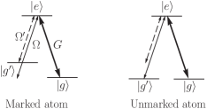
Figure 1: Linkage pattern for the individual atoms. The unmarked atoms have two degenerate ground states $|g\rangle$ and $|g^{\prime}\rangle$. One atom is marked with the state $|g^{\prime}\rangle$ shifted. The laser of Rabi frequency $\Omega^{\prime}$ (resp. $\Omega$) is resonant with the $g^{\prime}-e$ transition for the marked (resp. unmarked) atom(s). The cavity of Rabi frequency $G$ is resonant with the $g-e$ transition.

In this paper, we show an implementation of the adiabatic Grover algorithm based on a physical system, which is in principle scalable. This is, to our knowledge, the first proposed implementation of the adiabatic Grover algorithm. It is formulated with an Hamiltonian $H=H_{0}+V(t)$ where $H_{0}$ is considered as an oracle, and given, while $V(t)$ is slowly varying in time and such that there is an instantaneous eigenvector adiabatically connecting the initial superposition $|w\rangle$ to the marked state $|m\rangle$. We use an ensemble of $N$ identical three-level atoms trapped in a single-mode cavity of coupling frequency $G$, and driven by two lasers of Rabi frequencies $\Omega$ and $\Omega^{\prime}$. The atomic levels are in a $\Lambda$ configuration with two ground states $|g\rangle$ and $|g^{\prime}\rangle$ coupled to the excited state $|e\rangle$ by, respectively, the cavity and the two lasers (see Fig. 1). This can be realized in practice by considering Zeeman states and laser and cavity fields of appropriate polarizations. The states $|g^{\prime}\rangle$ of the $N$ atoms are considered as the database entries. The energy of the state $|g^{\prime}\rangle$ of the marked atom is shifted by an amount $\delta$ with respect to that of the unmarked atoms, which is set to zero. The states $|g\rangle$ allow for the coupling of all the atoms through the exchange of a single photon with the cavity (see Fig. 2a). The initial state we shall start from is the entangled state $|w\rangle\equiv|g^{\prime},0\rangle\equiv(1/\sqrt{N})\sum_{j=1}^{N}|g^{\prime}_{j},0\rangle$ featuring a collective single-photon atomic excitation. Note that the label of each atom is added as a subscript $1,\cdots,N$ and chosen so that the marked atom has tag $N$. Such a state can be prepared for instance before the marking of the atom using the stimulated Raman adiabatic passage (STIRAP) technique [14], exactly as shown in [15] to store single-photon quantum states. The process we introduce here allows one to drive adiabatically the population of the entangled state $|g^{\prime},0\rangle$, which corresponds to the superposition of both the marked state $|m\rangle\equiv|g^{\prime}_{N},0\rangle$ and an unmarked collective state $|g^{\prime}_{u},0\rangle$ that we introduce below, to the single marked state $|g^{\prime}_{N},0\rangle$ (see Fig. 2b). This process will be referred to as an inverse fractional stimulated Raman adiabatic passage (if-STIRAP) since it is a time inversion of the so-called fractional STIRAP (f-STIRAP) which transfers the population from a single state to a superposition of state [16]. This is implemented by first switching on $\Omega$ and $\Omega^{\prime}$ together and next switching off $\Omega^{\prime}$ before $\Omega$. The time to achieve such a process will then be shown to grow as $\sqrt{N}$ in order to satisfy adiabaticity.

Figure 2: (a) Coupling scheme in the cavity. The cavity $G$, laser $\Omega$, laser $\Omega^{\prime}$ Rabi frequency are featured by respectively thick, thin, and dashed arrows. (b) Equivalent scheme where the states $|g^{\prime}_{i},0\rangle$ (resp. $|e_{i},0\rangle$), $i=1,N-1$, of frame (a) form the collective unmarked ground state $|g^{\prime}_{u},0\rangle$ (resp. excited state $|e_{u},0\rangle$). The effective cavity Rabi frequency to the collective unmarked excited state is $\sqrt{N-1}G$.

The Hamiltonian describing the system of $N$ atoms is

$$H_{0}=\delta|g_{N}\rangle\langle g_{N}|+\omega\sum_{j=1}^{N}|e_{j}\rangle\langle e_{j}|.$$ (1)

We consider a cavity mode of frequency $\omega$ and coupling strength $G$ together with two lasers of frequencies $\omega$, $\omega-\delta$ and pulse shapes $\Omega(t)$, $\Omega^{\prime}(t)$ which do not grow with $N$. The resonant driving provided by the atoms-cavity-laser system is described by

$$V = \omega a^{\dagger}a+Ga\sum_{j=1}^{N}|e_{j}\rangle\langle g|$$ (2)

$$+ \left[\Omega e^{i\omega t}+\Omega^{\prime}e^{i(\omega-\delta)t}\right]\sum_{j=1}^{N}|g^{\prime}_{j}\rangle\langle e_{j}|+\rm{h.c.}$$

The full Hamiltonian $H=H_{0}+V$ has a photonic block diagonal structure. Each block is labeled by the number $k$ of photons in the cavity when the $N$ atoms are in their ground state $|g\rangle$. The corresponding multipartite state $|g_{1}\cdots g_{N}\rangle\otimes|k\rangle$ is denoted $|g,k\rangle$. All the states which are connected to $|g,k\rangle$ span a subspace whose projection operator is $P_{k}$. As each block is decoupled under $H$ from the other ones, $H=\sum_{k=0}P_{k}HP_{k}$, we shall focus on the block $P_{1}HP_{1}$ associated with a single photon in the cavity and show that it allows us to implement an adiabatic Grover search algorithm. The multipartite state $|g,1\rangle$ is connected by (2) to exactly two families of states as illustrated in Fig. 2a. Upon absorption of the cavity photon, the excited state $|e\rangle$ of any of the $N$ atoms, say atom $j$, can be reached while the other atoms remain in their ground state $|g\rangle$; the corresponding multipartite state is $|e_{j},0\rangle\equiv|g_{1}\cdots g_{j-1}e_{j}g_{j+1}\cdots\rangle\otimes|0\rangle$. The state $|e_{j},0\rangle$ can also be reached by absorption of one laser photon when any of the atoms, say atom $j$, is in the ground state $|g^{\prime}\rangle$ while the other atoms are in the ground state $|g\rangle$: $|g^{\prime}_{j},0\rangle\equiv|g_{1}\cdots g_{j-1}g^{\prime}_{j}g_{j+1}\cdots g_{N}\rangle\otimes|0\rangle$. In order to remove the oscillatory time dependence introduced by the laser we consider atomic states which are dressed by laser and cavity photons, and use the resonant transformation $R=e^{-i\delta t}|g^{\prime}_{N},0\rangle\langle g^{\prime}_{N},0|+e^{-i\omega t}|g,1\rangle\langle g,1|+\sum_{j=1}^{N}\left(|g^{\prime}_{j},0\rangle\langle g^{\prime}_{j},0|+e^{-i\omega t}|e_{j},0\rangle\langle e_{j},0|\right)$. As we shall see, the states which are relevant for the Grover search are the $N-1$ states $|g^{\prime}_{j},0\rangle$, which are unmarked, and the state $|g^{\prime}_{N},0\rangle$ which is marked. Among the unmarked atoms, none should play a privileged role. Hence we shall consider them collectively and label the corresponding state with a subscript $u$. We rewrite this Hamiltonian in a new basis which features the uniform superposition of the unmarked ground states

$$|g^{\prime}_{u},0\rangle=\frac{1}{\sqrt{N-1}}\sum_{j=1}^{N-1}|g^{\prime}_{j},0\rangle,$$ (3)

and the uniform superposition of the excited states associated with the unmarked atoms

$$|e_{u},0\rangle=\frac{1}{\sqrt{N-1}}\sum_{j=1}^{N-1}|e_{j},0\rangle.$$ (4)

This is achieved with the unitary transformation $W=|g^{\prime}_{N},0\rangle\langle g^{\prime}_{N},0|+|e_{N},0\rangle\langle e_{N},0|+|g,1\rangle\langle g,1|+\sum_{l,j=1}^{N-1}U_{l,j}\left(|g^{\prime}_{l},0\rangle\langle g^{\prime}_{j},0|+|e_{l},0\rangle\langle e_{j},0|\right)$ where $U$ is any unitary matrix such that the $(N-1)$ elements of one of its columns are equal. In this new basis, the part of the Hamiltonian restricted to the subspace spanned by the states $|g^{\prime}_{u},0\rangle,|g^{\prime}_{N},0\rangle,|g,1\rangle,|e_{u},0\rangle,|e_{N},0\rangle$ is decoupled from the rest. It reads

$$H_{1}=\left(\begin{array}[]{cc}0&V_{\ell}\\ V_{\ell}^{\dagger}&V_{\rm c}\end{array}\right),$$ (7)

with

$$V_{\ell}=\left(\begin{array}[]{ccc}0&\Sigma&0\\ 0&0&\Sigma^{\prime}\end{array}\right),\;V_{\rm c}=\left(\begin{array}[]{ccc}0&\sqrt{N-1}G&G\\ \sqrt{N-1}G&0&0\\ G&0&0\end{array}\right).$$ (13)

and $\Sigma=\Omega+e^{-i\delta t}\Omega^{\prime}$, $\Sigma^{\prime}=\Omega^{\prime}+e^{i\delta t}\Omega$. This Hamiltonian, whose derivation is exact, is represented in Fig. 2b. By means of a unitary transformation $T$, we diagonalize the block $V_{\rm c}$ which admits the eigenvalues $\gamma_{0}=0$ and $\gamma_{\pm}=\pm\sqrt{N}G$ whose associated eigenvectors read

$$|\gamma_{0}\rangle = \sqrt{1-\frac{1}{N}}|e_{N},0\rangle-\frac{1}{\sqrt{N}}|e_{u},0\rangle$$ (14)

$$|\gamma_{\pm}\rangle = \frac{1}{\sqrt{2}}\left(\frac{1}{\sqrt{N}}|e_{N},0\rangle+\sqrt{1-\frac{1}{N}}|e_{u},0\rangle\pm|g,1\rangle\right).$$

The new Hamiltonian reads, in the basis $|g^{\prime}_{u},0\rangle,|g^{\prime}_{N},0\rangle,|\gamma_{0}\rangle,|\gamma_{+}\rangle,|\gamma_{-}\rangle$ :

$$T^{\dagger}H_{1}T=\left(\begin{array}[]{cc}A&B\\ B^{\dagger}&C\end{array}\right),$$ (17)

with

$$A = \frac{1}{\sqrt{N}}\left(\begin{array}[]{ccc}0&0&-\Sigma\\ 0&0&\sqrt{N-1}\Sigma^{\prime}\\ -\Sigma^{*}&\sqrt{N-1}\,{\Sigma^{\prime}}^{*}&0\end{array}\right)$$ (21)

$$B = \frac{1}{\sqrt{2N}}\left(\begin{array}[]{ccc}\sqrt{N-1}\Sigma&\sqrt{N-1}\Sigma\\ \Sigma^{\prime}&\Sigma^{\prime}\\ 0&0\end{array}\right)$$ (25)

$$C = \sqrt{N}\left(\begin{array}[]{cc}G&0\\ 0&-G\end{array}\right).$$ (28)

The time evolution of the non-resonant components in $\Sigma$ and $\Sigma^{\prime}$ is much faster than the evolution of $\Omega$ and $\Omega^{\prime}$ which occurs over a time scale $\mathcal{T}\gg\delta^{-1}$. Hence it is justified to replace these contributions by their vanishing average values over times $\delta^{-1}\ll\tau\ll\mathcal{T}$: $\overline{\Sigma}\simeq\Omega$ and $\overline{\Sigma^{\prime}}\simeq\Omega^{\prime}$, where $\overline{f}(t)=\frac{1}{\tau}\int_{t}^{t+\tau}duf(u)$. This is the resonant approximation. Similarily, the unitary evolution of $C$ is much faster than that of $A$ if $\Omega_{\rm peak}/NG\ll 1$ since the respective eigenvalues scale as $\sqrt{N}G$ and $\Omega_{\rm peak}/\sqrt{N}$ where $\Omega_{\rm peak}$ is the peak amplitude of the pulse $\Omega$. Upon performing an adiabatic elimination we thus obtain an effective Hamiltonian $H_{{\rm eff}}=\overline{A}-\overline{B}C^{-1}\overline{B}^{\dagger}$ which contains all the contributions up to order $(\Omega_{\rm peak}/NG)^{4}$. In the basis $|g^{\prime}_{N},0\rangle,|\gamma_{0}\rangle,|g^{\prime}_{u},0\rangle$, the effective Hamiltonian reads

$$H_{{\rm eff}}=\frac{1}{\sqrt{N}}\left(\begin{array}[]{ccc}0&\sqrt{N-1}\Omega^{\prime}&0\\ \sqrt{N-1}\Omega^{\prime}&0&-\Omega\\ 0&-\Omega&0\\ \end{array}\right).$$ (32)

Our aim is to transfer adiabatically the population from an initial state $|g^{\prime},0\rangle$ which gives no privileged role to any of the $N$ states $|g^{\prime}_{j},0\rangle$ to a final state which coincides with the marked state $|g^{\prime}_{N},0\rangle$ in a time which scales as $\sqrt{N}$. The population transfer mechanism is most easily revealed in the basis of the instantaneous eigenstates of $H_{{\rm eff}}(t)$

$$|0\rangle(t) = \cos\theta(t)\ |g^{\prime}_{N},0\rangle-\sin\theta(t)\ |g^{\prime}_{u},0\rangle$$ (33)

$$|\pm\rangle(t) = \frac{1}{\sqrt{2}}\left(\sin\theta(t)\ |g^{\prime}_{N},0\rangle+\cos\theta(t)\ |g^{\prime}_{u},0\rangle\pm|\gamma_{0}\rangle\right),$$

pertaining to the eigenvalues 0 and $\pm\Lambda(t)$ where

$$\Lambda(t)=\frac{1}{\sqrt{N}}\sqrt{(N-1){\Omega^{\prime}}^{2}(t)+\Omega^{2}(t)}.$$ (34)

The instantaneous angle $\theta(t)$ is defined through the relation

$$\tan\theta(t) = -\sqrt{N-1}\frac{\Omega^{\prime}(t)}{\Omega(t)}.$$ (35)

Requiring the instantaneous eigenstate (33) to coincide at the initial time $t_{i}$ with the uniform superposition

$$|g^{\prime},0\rangle=\frac{1}{\sqrt{N}}|g^{\prime}_{N},0\rangle+\sqrt{1-\frac{1}{N}}|g^{\prime}_{u},0\rangle,$$ (36)

and at the final time with the marked state $|g^{\prime}_{N},0\rangle$ entails that

$$\tan\theta(t_{\rm i})=-\sqrt{N-1},\quad\tan\theta(t_{\rm f})=0.$$ (37)

This implies that the two pulses must be switched on simultaneously, $\Omega^{\prime}(t_{\rm i})=\Omega(t_{\rm i})$ and that the pulse $\Omega^{\prime}$ is to be turned off before $\Omega$. In the adiabatic representation (33), the Hamiltonian (32) reads

$$H_{{\rm eff}}^{\rm ad}=\left(\begin{array}[]{ccc}\Lambda&\frac{i}{\sqrt{2}}\dot{\theta}&0\\ -\frac{i}{\sqrt{2}}\dot{\theta}&0&-\frac{i}{\sqrt{2}}\dot{\theta}\\ 0&\frac{i}{\sqrt{2}}\dot{\theta}&-\Lambda\\ \end{array}\right),$$ (41)

where $\dot{\theta}=\frac{1}{1+\tan^{2}\theta}\frac{d}{dt}\tan\theta$. In the adiabatic regime, the transitions between instantaneous eigenstates are negligible. This will be achieved if the Hamiltonian varies sufficiently slowly in time so as to keep $\dot{\theta}\ll\Lambda$. On the other hand, we wish to control the process duration and, in particular, to prevent it from becoming arbitrary large. For that purpose, as proposed in [13], we choose to require $\dot{\theta}$ and $\Lambda$ to be in a constant (small) ratio $\varepsilon$ at all times, independently of $N$:

$$\dot{\theta}=\varepsilon\Lambda.$$ (42)

This choice is adopted for the sake of clarity, since in this case the scaling can be analytically determined and proven to scale as $\sqrt{N}$. We have investigated the robustness of this approach. Given a laser pulse $\Omega$, this equation will allow us to determine the pulse $\Omega^{\prime}$ which is needed to remain in the instantaneous eigenstate $|0\rangle(t)$ with a probability larger than $1-\varepsilon^{2}$ throughout the process, starting from the uniform superposition $|0\rangle(t_{{\rm i}})=|w\rangle$, and ending up in the marked state $|0\rangle(t_{{\rm f}})=|g^{\prime}_{N},0\rangle$ after some time $\mathcal{T}=t_{{\rm f}}-t_{{\rm i}}$. Indeed, rewriting (34) with (35) as $\Lambda=\frac{1}{\sqrt{N}}\sqrt{1+\tan^{2}\theta}\Omega$, we obtain from (42) a differential equation for $\tan\theta$, i. e., for the ratio $\Omega^{\prime}/\Omega$. Its solution satisfying the initial condition (37) reads

$$\frac{\Omega^{\prime}(t)}{\Omega(t)}=\frac{1-\frac{\varepsilon{\mathcal{A}}(t)}{\sqrt{N-1}}}{\sqrt{1+\varepsilon{\mathcal{A}}(t)\{2\sqrt{N-1}-\varepsilon{\mathcal{A}}(t)\}}},$$ (43)

where we define ${\mathcal{A}}(t)\equiv\int_{t_{{\rm i}}}^{t}du\Omega(u)$. The process duration $\mathcal{T}$ is obtained implicitly upon specifying that at time $t_{{\rm f}}$ the ratio on the left side of (43) vanishes:

$$\varepsilon{\mathcal{A}}(\mathcal{T})=\sqrt{N-1}.$$ (44)

Expressing the total area of the pulse $\Omega$ in terms of its average amplitude $\overline{\Omega}$, ${\mathcal{A}}(\mathcal{T})=\overline{\Omega}\mathcal{T}$, we arrive at

$$\overline{\Omega}\mathcal{T}=\frac{\sqrt{N-1}}{\varepsilon}.$$ (45)

This shows that, for a constant average amplitude (i.e. independent of $N$), the duration scales as $\sqrt{N}$. Note that we can equivalently increase the average amplitude as $\sqrt{N}$ for a constant time $\mathcal{T}$. We can determine from (43) that $\overline{\Omega}^{\prime}\mathcal{T}$ grows as $(\sqrt{N}-1)/\sqrt{N-1}$, i.e., as $O(N^{0})$.

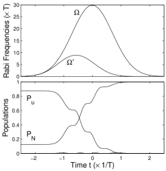
Figure 3: Numerical dynamics with the effective Hamiltonian (32) for $N=8$, $\varepsilon=0.05$ and a Gaussian Rabi frequency $\Omega(t)=\Omega_{\rm peak}e^{-(t/T)^{2}}$ with $\Omega_{\rm peak}T=\sqrt{N-1}/(\varepsilon\sqrt{\pi})$ [in order to satisfy (37) and (42)]. $\Omega^{\prime}(t)$ is determined from (43). Top: Rabi frequencies. Bottom: Populations of the collective unmarked state $P_{u}(t)\equiv|\langle g^{\prime}_{u},0|\phi\rangle(t)|^{2}$, and of the marked state $P_{N}(t)\equiv|\langle g^{\prime}_{N},0|\phi\rangle(t)|^{2}$, where $|\phi\rangle(t)$ is the dynamical state vector.

Figure 3 displays the pulses and the population dynamics resulting from (43) with $N=8$, $\varepsilon=0.05$ and a Gaussian pulse $\Omega$ of characteristic duration $T$. As predicted, the transfer to the marked state is very efficient. The very low transient population in the excited states stems from the fact that the dynamics is expected to remain in the instantaneous decoherence-free eigenstate $|0\rangle(t)$ in the adiabatic limit. Notice that the choice (42), which leads to the seemingly complicated pulse relation (43), gives in practice a simple smooth bell-shaped pulse (see Fig. 3). We have numerically checked that the efficiency of the transfer is, as expected, preserved for a wide range of $N$ with $\Omega_{\rm peak}T$ growing as $\sqrt{N}$ and an almost constant $\Omega^{\prime}_{\rm peak}T$. In conclusion, we have proposed the first physical implementation of the adiabatic Grover search using a cavity-laser-atom system and robust processes related to STIRAP. The calculation has been conducted with pulses based on the constraint (42) that has allowed us to prove the scaling analytically. We have checked the robustness of the $\sqrt{N}$ scaling by numerical simulations using other less restrictive adiabatic pulse shapes satisfying (37). The authors are grateful to N. J. Cerf and H.-R. Jauslin for useful discussions and acknowledge the support from the EU projects COVAQIAL and QAP, from the Belgian government programme IUAP under grant V-18, and from the Conseil Régional de Bourgogne.

References

• [1] L. K. Grover, Phys. Rev. Lett, 79, 325 (1997).
• [2] I. L. Chuang, N. Gershenfeld, and M. Kubinec, Phys. Rev. Lett. 80, 3408 (1998).
• [3] J. A. Jones, M. Mosca, and R. H. Hansen, Nature (London) 393, 344 (1998).
• [4] N. Bhattacharya, H. B. van Linden van den Heuvell, and R. J. C. Spreeuw, Phys. Rev. Lett. 88, 137901 (2002).
• [5] P. Walther, K. J. Resch, T. Rudolph, E. Schenck, H. Weinfurter, V. Vedral, M. Aspelmeyer, and A. Zeilinger, Nature (London) 434, 169 (2005).
• [6] K.-A. Brickman, P. C. Haljan, P. J. Lee, M. Acton, L. Deslauriers, and C. Monroe, Phys. Rev. A 72, 050306(R) (2005).
• [7] F. Yamaguchi, P. Milman, M. Brune, J. M. Raimond, and S. Haroche, Phys. Rev. A 66, 010302(R) (2002).
• [8] Z. J. Deng, M. Feng, and K. L. Gao, Phys. Rev. A 72, 034306 (2005).
• [9] E. Farhi and S. Gutmann, Phys. Rev. A 57, 2403 (1998).
• [10] V. L. Ermakov and B. M. Fung, Phys. Rev. A 66, 042310 (2002).
• [11] E. Farhi, J. Goldstone, S. Gutmann, and M. Sipser, e-print quant-ph/0001106.
• [12] A. M. Childs, E. Farhi, and J. Preskill, Phys. Rev. A 65, 012322 (2001).
• [13] J. Roland and N. J. Cerf, Phys. Rev. A 65, 042308 (2002).
• [14] N. V. Vitanov, T. Halfmann, B. W. Shore, and K. Bergmann, Annu. Rev. Phys. Chem. 52, 763 (2001).
• [15] M. Fleischhauer and M. D. Lukin, Phys. Rev. A 65, 022314 (2002).
• [16] N. V. Vitanov, K.-A. Suominen, and B. W. Shore, J. Phys. B 32, 4535 (1999).