FTUAM-07/10

IFT-UAM/CSIC-07-28

LPT-ORSAY-07-51

μe𝜇𝑒\mu\,-\,e conversion in nuclei within the CMSSM seesaw: universality versus non-universality

E. Arganda a, M. J. Herrero a and A. M. Teixeira b

aDepartamento de Física Teórica C-XI and Instituto de Física Teórica C-XVI,
Universidad Autónoma de Madrid, Cantoblanco, E-28049 Madrid, Spain

bLaboratoire de Physique Théorique, UMR 8627

Université de Paris-Sud XI, Bâtiment 201, F-91405 Orsay Cedex, France

Abstract

In this paper we study μe𝜇𝑒\mu-e conversion in nuclei within the context of the Constrained Minimal Supersymmetric Standard Model, enlarged by three right handed neutrinos and their supersymmetric partners, and where the neutrino masses are generated via a seesaw mechanism. Two different scenarios with either universal or non-universal soft supersymmetry breaking Higgs masses at the gauge coupling unification scale are considered. In the first part we present a complete one-loop computation of the conversion rate for this process that includes the photon-, Z𝑍Z-boson, and Higgs-boson penguins, as well as box diagrams, and compare their size in the two considered scenarios. Then, in these two scenarios we analyse the relevance of the various parameters on the conversion rates, particularly emphasising the role played by the heavy neutrino masses, tanβ𝛽\tan\beta, and especially θ13subscript𝜃13\theta_{13}. In the case of hierachical heavy neutrinos, an extremely high sensitivity of the rates to θ13subscript𝜃13\theta_{13} is indeed found. The last part of this work is devoted to the study of the interesting loss of correlation between the μe𝜇𝑒\mu-e conversion and μeγ𝜇𝑒𝛾\mu\to e\gamma rates that occurs in the non-universal scenario. In the case of large tanβ𝛽\tan\beta and light H0superscript𝐻0H^{0} Higgs boson, an enhanced ratio of the μe𝜇𝑒\mu-e to μeγ𝜇𝑒𝛾\mu\to e\gamma rates, with respect to the universal case is found, and this could be tested with the future experimental sensitivities.

1 Introduction

Neutrino physics, in particular neutrino oscillations and the measured neutrino mass differences, strongly manifest that Nature does not conserve the lepton flavour quantum number in the neutrino sector [1, 2]. However, it is not known yet if lepton flavour violation (LFV) also occurs in the charged lepton sector. If such is the case, one still has to address if LFV in the neutral and charged lepton sectors arises from a common or different origin. It is well known that if the Standard Model of Particle Physics (SM) is minimally extended in order to accommodate the present data on neutrino masses and mixings, the corresponding loop induced LFV in the charged lepton sector (exclusively induced from neutrino oscillations) is extremely tiny and hopeless to be experimentally observed. Therefore, a potential future measurement of LFV in the charged lepton sector will provide a unique insight into the nature of new physics beyond the SM (for a review, see [3]).

Among the various candidates for physics beyond the SM that produce potentially observable effects in LFV processes, one of the most appealing are Supersymmetric (SUSY) extensions of the SM, where a seesaw mechanism [4, 5] is implemented to generate neutrino masses. In these SUSY-seesaw models a new source of LFV appears in the off-diagonal elements of the slepton mass matrices, which can be radiatively generated. The size of these elements is governed by the strength of the neutrino Yukawa couplings and, in the case of Majorana neutrinos, the latter can be large, of the order of one. The LFV effects in the charged lepton processes are then induced by flavour violating slepton-lepton interactions, appearing in SUSY-loop diagrams mediated by sleptons [6].

Concerning the LFV processes, in our work we will focus on those which involve flavour transitions between the first and second generation of charged leptons. At present, the most relevant μe𝜇𝑒\mu-e flavour violating processes are μeγ𝜇𝑒𝛾\mu\to e\gamma, μ3e𝜇3𝑒\mu\to 3e and μe𝜇𝑒\mu-e conversion in nuclei. The current experimental bounds on the muon decays are BR(μeγ)<1.2×10¹¹𝜇𝑒𝛾1.2superscript1011(\mu\to e\gamma)<1.2\times 10^{-11} [7] and BR(μ3e)<1.0×10¹²𝜇3𝑒1.0superscript1012(\mu\to 3e)<1.0\times 10^{-12} [8]. Regarding μe𝜇𝑒\mu-e conversion in heavy nuclei, the most stringent constraints arise for Titanium and Gold, respectively with CR(μe𝜇𝑒\mu-e, Ti)<4.3×10¹²absent4.3superscript1012<4.3\times 10^{-12} [9] and CR(μe𝜇𝑒\mu-e, Au)<7×10¹³absent7superscript1013<7\times 10^{-13} [10]. In the future, one expects significant improvements in the sentitivies to these LFV rates. For instance, MEG aims at reaching a sensitivity for μeγ𝜇𝑒𝛾\mu\to e\gamma of 1013superscript101310^{-13} [11] in the very near future, which could further be improved to 1014superscript101410^{-14} in the next 4-5 years [12]. Although the situation for BR(μ3e)𝜇3𝑒(\mu\to 3e) is less certain, one does not expect the sensitivities to better 10131014superscript1013superscript101410^{-13}-10^{-14} [12]. Undoubtedly, the most challenging prospects concern the experimental sensitivities to μe𝜇𝑒\mu-e conversion in Titanium nuclei. The dedicated J-PARC experiment PRISM/PRIME has anounced a remarkable improvement, albeit in a farer future, of 1018superscript101810^{-18} [13].

In this paper we will focus on μe𝜇𝑒\mu-e conversion in nuclei, working in the context of the Minimal Supersymmetric Standard Model (MSSM) enlarged by three right handed neutrinos and their corresponding SUSY partners, where a type-I seesaw mechanism [4] is implemented. To reduce the number of unknown parameters in the SUSY sector, we choose to work in the so-called constrained MSSM (CMSSM)(for a review see for instance [14]), assuming universality of the soft-SUSY breaking parameters at the scale of gauge coupling unification, MX2×1016similar-tosubscript𝑀𝑋2superscript1016M_{X}\sim 2\times 10^{16} GeV. An interesting departure from the CMSSM-seesaw can be obtained by relaxing the universality hypothesis for the soft SUSY breaking masses of the Higgs sector. This partially constrained MSSM is commonly referred to as the Non Universal Higgs Mass (NUHM) scenario [15], and its enlarged version (including right handed neutrinos and sneutrinos) will be here designated NUHM-seesaw.

Within the context of the CMSSM- and NUHM-seesaw, we conduct here a thourough analysis of the predictions for the μe𝜇𝑒\mu-e conversion rates in nuclei. The present computation is the first to include the full set of SUSY one-loop diagrams (photon, Z𝑍Z- and Higgs-boson mediated, as well as box diagrams), and to be strictly done in terms of physical eigenstates for the exchanged SUSY particles. For all scenarios here addressed, we obtain the low-energy parameters by numerically solving the full renormalisation group equations (RGEs), including the neutrino and sneutrino sectors. The photon and Z𝑍Z-boson mediated penguins, as well as the vector contributions from box diagrams were first computed in the CMSSM-seesaw in [16]. Here we have confirmed their analytical results for the photon-mediated and box contributions, correcting the analytical expressions for the Z𝑍Z-boson mediated processes. We further added the scalar contributions from box diagrams and the Higgs-mediated contributions, and improved the computation, by considering in the numerical analysis the possibility of either degenerate or hierarchical heavy neutrino spectrum, and by fitting the light neutrino parameters to the present data.

The effects of the Higgs-mediated contribution on μe𝜇𝑒\mu-e conversion rates were firstly investigated in [17], in the context of a SUSY-seesaw with degenerate heavy neutrinos, working in the effective Lagrangian approximation and in the SU(2)L×U(1)Y𝑆𝑈subscript2𝐿𝑈subscript1𝑌SU(2)_{L}\times U(1)_{Y} limit. It was observed that the Higgs-mediated LFV diagrams could provide the dominant contribution for the large tanβ𝛽\tan\beta regime and for small masses of the heavy Higgs scalar, owing to a tan6βsuperscript6𝛽\tan^{6}{\beta} enhancement and (mH0)4superscriptsubscript𝑚superscript𝐻04(m_{H^{0}})^{-4} dependence of the conversion rates. By comparing the latter with the corresponding μeγ𝜇𝑒𝛾\mu\to e\gamma rates for large universal SUSY-breaking mass values, M0,M1/2𝒪(1M_{0},M_{1/2}\sim\mathcal{O}(1 TeV), they further showed that the ratio of observables CR(μe,(\mu-e, Al)/BR(μeγ)𝜇𝑒𝛾(\mu\to e\gamma) could be enhanced from a value of 𝒪(α)𝒪𝛼\mathcal{O}(\alpha) (within the usual dominant photon-mediated case) to 𝒪(101)𝒪superscript101\mathcal{O}(10^{-1}) for extreme values of tanβ=60𝛽60\tan\beta=60, MR=1014subscript𝑀𝑅superscript1014M_{R}=10^{14} GeV and mH0100similar-tosubscript𝑚superscript𝐻0100m_{H^{0}}\sim 100 GeV.

In the present work we will explore in full detail the various contributions to the μe𝜇𝑒\mu-e conversion rates and study the dependence on all parameters entering in the considered MSSM-seesaw framework. In addition to the relevant role played by the mass of the right handed neutrinos, mNisubscript𝑚subscript𝑁𝑖m_{N_{i}}, the soft masses M0subscript𝑀0M_{0}, M1/2subscript𝑀12M_{1/2} (and MH1,2subscript𝑀subscript𝐻12M_{H_{1,2}} for the NUHM-seesaw), and tanβ𝛽\tan\beta, we will show that the light neutrino mixing angle θ13subscript𝜃13\theta_{13} has an important impact on CR(μe,Nucleus(\mu-e,\text{Nucleus}). The conversion rates turn out to be very sensitive to this angle, varying in many orders of magnitude (up to five in the case of hierarchical heavy neutrinos) for θ13subscript𝜃13\theta_{13} values within the present experimentally allowed region 0θ1310superscript0subscript𝜃13superscript100^{\circ}\leq\theta_{13}\leq 10^{\circ} [18]. We will further verify that with the future sensitivity of JPARC (𝒪(1018)𝒪superscript1018\mathcal{O}(10^{-18})[13] most of the parameter space could be covered.

On the other hand, the comparison between the predictions obtained for the CMSSM-seesaw and the NUHM-seesaw cases will allow us to draw interesting conclusions about the departure from the strongly correlated behaviour of CR(μe,Nucleus)𝜇𝑒Nucleus(\mu-e,\text{Nucleus}) and BR(μeγ)𝜇𝑒𝛾(\mu\to e\gamma), as predicted in photon-dominated scenarios (as is the case of the CMSSM-seesaw). In the latter scenario, the ratio of the two rates was found to be at most 1/16011601/160 for tanβ=50𝛽50\tan\beta=50 [19]. In contrast, we will discuss here particular scenarios in the NUHM-seesaw, where the ratio CR(μe(\mu-e, Ti)/BR(μeγ)𝜇𝑒𝛾(\mu\to e\gamma) is indeed enhanced with respect to the universal case, by as much as one order of magnitude, in agreement with the approximate results of [17].

One of the most challenging tasks in this μe𝜇𝑒\mu-e conversion process will be to disantangle between the different scenarios for new physics if a measurement is finally obtained. Indeed, it has been already noticed in early works [20] that μe𝜇𝑒\mu-e conversion could constrain new physics more stringently than μeγ𝜇𝑒𝛾\mu\to e\gamma. We will see here that this is the case in the NUHM scenario. Furthermore, we will also show that, with the expected sensitivities for Titanium of 𝒪(1018\mathcal{O}(10^{-18}), one could distinguish CMSSM- from NUHM- seesaw scenarios by extracting the scalar contribution to the CR(μe(\mu-e, Ti) rates.

The paper is organised as follows. In Section 2 we review the most relevant features of the SUSY-seesaw scenario. The analytical results of the μe𝜇𝑒\mu-e conversion rates are presented in Section 3. Section 4 is devoted to the numerical results for both CMSSM-seesaw and NUHM-seesaw scenarios. An extensive discussion about the sensitivities to the various parameters in these two scenarios is also included. Finally, the conclussions are summarised in Section 5.

2 The SUSY-seesaw scenario

The leptonic superpotential containing the relevant terms to describe a type-I SUSY seesaw is given by

W=N^cYνL^H^2+E^cYlL^H^1+12N^cmMN^c,𝑊superscript^𝑁𝑐subscript𝑌𝜈^𝐿subscript^𝐻2superscript^𝐸𝑐subscript𝑌𝑙^𝐿subscript^𝐻112superscript^𝑁𝑐subscript𝑚𝑀superscript^𝑁𝑐W\,=\,\hat{N}^{c}\,Y_{\nu}\,\hat{L}\,\hat{H}_{2}\,+\,\hat{E}^{c}\,Y_{l}\,\hat{L}\,\hat{H}_{1}\,+\,\frac{1}{2}\,\hat{N}^{c}\,m_{M}\,\hat{N}^{c}\,, (1)

where N^csuperscript^𝑁𝑐\hat{N}^{c} are the additional superfields that contain the three right-handed neutrinos νRisubscript𝜈subscript𝑅𝑖\nu_{R_{i}} and their scalar partners ν~Risubscript~𝜈subscript𝑅𝑖\tilde{\nu}_{R_{i}}. The lepton Yukawa couplings Yl,νsubscript𝑌𝑙𝜈Y_{l,\nu} and the Majorana mass mMsubscript𝑚𝑀m_{M} are 3×3333\times 3 matrices in lepton flavour space. From now on, we will assume that we are in a basis where Ylsubscript𝑌𝑙Y_{l} and mMsubscript𝑚𝑀m_{M} are diagonal.

After electroweak (EW) symmetry breaking, the charged lepton and Dirac neutrino mass matrices can be written as

ml=Ylv1,mD=Yνv2,formulae-sequencesubscript𝑚𝑙subscript𝑌𝑙subscript𝑣1subscript𝑚𝐷subscript𝑌𝜈subscript𝑣2m_{l}\,=\,Y_{l}\,\,v_{1}\,,\quad\quad m_{D}\,=\,Y_{\nu}\,v_{2}\,, (2)

where visubscript𝑣𝑖v_{i} are the vacuum expectation values (VEVs) of the neutral Higgs scalars, with v1(2)=vcos(sin)βsubscript𝑣12𝑣𝛽v_{1(2)}=\,v\,\cos(\sin)\beta and v=174𝑣174v=174 GeV.

The 6×6666\times 6 neutrino mass matrix is given by

Mν=(0mDTmDmM).superscript𝑀𝜈0superscriptsubscript𝑚𝐷𝑇subscript𝑚𝐷subscript𝑚𝑀M^{\nu}\,=\,\left(\begin{array}[]{cc}0&m_{D}^{T}\\ m_{D}&m_{M}\end{array}\right)\,. (3)

The eigenvalues of Mνsuperscript𝑀𝜈M^{\nu} are the masses of the six physical Majorana neutrinos. In the seesaw limit, the three right-handed masses are much heavier than the EW scale, mMivmuch-greater-thansubscript𝑚subscript𝑀𝑖𝑣m_{M_{i}}\,\gg\,v, and one obtains three light and three heavy states, νisubscript𝜈𝑖\nu_{i} and Nisubscript𝑁𝑖N_{i}, respectively.

Block-diagonalisation of the neutrino mass matrix of Eq. (3), leads (at lowest order in the (mD/mM)nsuperscriptsubscript𝑚𝐷subscript𝑚𝑀𝑛(m_{D}/m_{M})^{n} expansion) to the standard seesaw equation for the light neutrino mass matrix,

mν=mDTmM1mD.subscript𝑚𝜈superscriptsubscript𝑚𝐷𝑇superscriptsubscript𝑚𝑀1subscript𝑚𝐷m_{\nu}\,=\,-m_{D}^{T}m_{M}^{-1}m_{D}\,. (4)

Since we are working in a basis where mMsubscript𝑚𝑀m_{M} is diagonal, the heavy eigenstates are then given by

mNdiag=mM=diag(mN1,mN2,mN3).superscriptsubscript𝑚𝑁diagsubscript𝑚𝑀diagsubscript𝑚subscript𝑁1subscript𝑚subscript𝑁2subscript𝑚subscript𝑁3m_{N}^{\text{diag}}\,=\,m_{M}\,=\,\text{diag}\,(m_{N_{1}},m_{N_{2}},m_{N_{3}})\,. (5)

The matrix mνsubscript𝑚𝜈m_{\nu} can be diagonalised by the Maki-Nakagawa-Sakata unitary matrix UMNSsubscript𝑈MNSU_{\text{MNS}} [21, 22], leading to the following masses for the light physical states

mνdiagsuperscriptsubscript𝑚𝜈diag\displaystyle m_{\nu}^{\text{diag}} =UMNSTmνUMNS=diag(mν1,mν2,mν3).absentsuperscriptsubscript𝑈MNS𝑇subscript𝑚𝜈subscript𝑈MNSdiagsubscript𝑚subscript𝜈1subscript𝑚subscript𝜈2subscript𝑚subscript𝜈3\displaystyle\,=\,U_{\text{MNS}}^{T}\,m_{\nu}\,U_{\text{MNS}}\,=\,\text{diag}\,(m_{\nu_{1}},m_{\nu_{2}},m_{\nu_{3}})\,. (6)

Here we use the standard parameterisation for UMNSsubscript𝑈MNSU_{\mathrm{MNS}} given by

UMNS=(c12c13s12c13s13eiδs12c23c12s23s13eiδc12c23s12s23s13eiδs23c13s12s23c12c23s13eiδc12s23s12c23s13eiδc23c13).V,formulae-sequencesubscript𝑈MNSsubscript𝑐12subscript𝑐13subscript𝑠12subscript𝑐13subscript𝑠13superscript𝑒𝑖𝛿subscript𝑠12subscript𝑐23subscript𝑐12subscript𝑠23subscript𝑠13superscript𝑒𝑖𝛿subscript𝑐12subscript𝑐23subscript𝑠12subscript𝑠23subscript𝑠13superscript𝑒𝑖𝛿subscript𝑠23subscript𝑐13subscript𝑠12subscript𝑠23subscript𝑐12subscript𝑐23subscript𝑠13superscript𝑒𝑖𝛿subscript𝑐12subscript𝑠23subscript𝑠12subscript𝑐23subscript𝑠13superscript𝑒𝑖𝛿subscript𝑐23subscript𝑐13𝑉U_{\text{MNS}}=\left(\begin{array}[]{ccc}c_{12}\,c_{13}&s_{12}\,c_{13}&s_{13}\,e^{-i\delta}\\ -s_{12}\,c_{23}\,-\,c_{12}\,s_{23}\,s_{13}\,e^{i\delta}&c_{12}\,c_{23}\,-\,s_{12}\,s_{23}\,s_{13}\,e^{i\delta}&s_{23}\,c_{13}\\ s_{12}\,s_{23}\,-\,c_{12}\,c_{23}\,s_{13}\,e^{i\delta}&-c_{12}\,s_{23}\,-\,s_{12}\,c_{23}\,s_{13}\,e^{i\delta}&c_{23}\,c_{13}\end{array}\right)\,.\,V\,, (7)

with

V=diag(eiϕ12,eiϕ22,1),𝑉diagsuperscript𝑒𝑖subscriptitalic-ϕ12superscript𝑒𝑖subscriptitalic-ϕ221V\,=\,\text{diag}\,(e^{-i\frac{\phi_{1}}{2}},e^{-i\frac{\phi_{2}}{2}},1)\,, (8)

where cijcosθijsubscript𝑐𝑖𝑗subscript𝜃𝑖𝑗c_{ij}\equiv\cos\theta_{ij}, sijsinθijsubscript𝑠𝑖𝑗subscript𝜃𝑖𝑗s_{ij}\equiv\sin\theta_{ij}. θijsubscript𝜃𝑖𝑗\theta_{ij} are the neutrino flavour mixing angles, δ𝛿\delta is the Dirac phase and ϕ1,2subscriptitalic-ϕ12\phi_{1,2} are the Majorana phases.

In view of the above, the seesaw equation (4) can be solved for mDsubscript𝑚𝐷m_{D} as [23]

mD=imNdiagRmνdiagUMNS,subscript𝑚𝐷𝑖subscriptsuperscript𝑚diag𝑁𝑅subscriptsuperscript𝑚diag𝜈subscriptsuperscript𝑈MNSm_{D}\,=\,i\sqrt{m^{\text{diag}}_{N}}\,R\,\sqrt{m^{\text{diag}}_{\nu}}\,U^{\dagger}_{\text{MNS}}\,, (9)

where R𝑅R is a generic complex orthogonal 3×3333\times 3 matrix that encodes the possible extra neutrino mixings (associated with the right-handed sector) in addition to the ones in UMNSsubscript𝑈MNSU_{\text{MNS}}. R𝑅R can be parameterised in terms of three complex angles, θisubscript𝜃𝑖\theta_{i} (i=1,2,3)𝑖123(i=1,2,3) as [23]

R=(c2c3c1s3s1s2c3s1s3c1s2c3c2s3c1c3s1s2s3s1c3c1s2s3s2s1c2c1c2),𝑅subscript𝑐2subscript𝑐3subscript𝑐1subscript𝑠3subscript𝑠1subscript𝑠2subscript𝑐3subscript𝑠1subscript𝑠3subscript𝑐1subscript𝑠2subscript𝑐3subscript𝑐2subscript𝑠3subscript𝑐1subscript𝑐3subscript𝑠1subscript𝑠2subscript𝑠3subscript𝑠1subscript𝑐3subscript𝑐1subscript𝑠2subscript𝑠3subscript𝑠2subscript𝑠1subscript𝑐2subscript𝑐1subscript𝑐2R\,=\,\left(\begin{array}[]{ccc}c_{2}\,c_{3}&-c_{1}\,s_{3}\,-\,s_{1}\,s_{2}\,c_{3}&s_{1}\,s_{3}\,-\,c_{1}\,s_{2}\,c_{3}\\ c_{2}\,s_{3}&c_{1}\,c_{3}\,-\,s_{1}\,s_{2}\,s_{3}&-s_{1}\,c_{3}\,-\,c_{1}\,s_{2}\,s_{3}\\ s_{2}&s_{1}\,c_{2}&c_{1}\,c_{2}\end{array}\right)\,, (10)

with cicosθisubscript𝑐𝑖subscript𝜃𝑖c_{i}\equiv\cos\theta_{i}, sisinθisubscript𝑠𝑖subscript𝜃𝑖s_{i}\equiv\sin\theta_{i}. Eq. (9) is a convenient means of parameterising our ignorance of the full neutrino Yukawa couplings, while at the same time allowing to accommodate the experimental data. Notice that it is only valid at the right-handed neutrino scales mMsubscript𝑚𝑀m_{M}, so that the quantities appearing in Eq. (9) are the renormalised ones, mνdiag(mM)subscriptsuperscript𝑚diag𝜈subscript𝑚𝑀m^{\text{diag}}_{\nu}\,(m_{M}) and UMNS(mM)subscript𝑈MNSsubscript𝑚𝑀U_{\text{MNS}}\,(m_{M}).

We shall focus on the scenario where the light neutrinos are hierarchical, and we will assume a normal hierarchy,

mν1mν2mν3.much-less-thansubscript𝑚subscript𝜈1subscript𝑚subscript𝜈2much-less-thansubscript𝑚subscript𝜈3\displaystyle m_{\nu_{1}}\,\ll\,m_{\nu_{2}}\,\ll\,m_{\nu_{3}}\,. (11)

The masses mν2,3subscript𝑚subscript𝜈23m_{\nu_{2,3}} can be written in terms of the lightest mass mν1subscript𝑚subscript𝜈1m_{\nu_{1}}, and of the solar and atmospheric mass-squared differences as

mν22=Δmsol2+mν12,superscriptsubscript𝑚subscript𝜈22Δsuperscriptsubscript𝑚sol2superscriptsubscript𝑚subscript𝜈12\displaystyle m_{\nu_{2}}^{2}\,=\,\Delta m_{\text{sol}}^{2}\,+\,m_{\nu_{1}}^{2}\,,
mν32=Δmatm2+mν12.superscriptsubscript𝑚subscript𝜈32Δsuperscriptsubscript𝑚atm2superscriptsubscript𝑚subscript𝜈12\displaystyle m_{\nu_{3}}^{2}\,=\,\Delta m_{\text{atm}}^{2}\,+\,m_{\nu_{1}}^{2}\,. (12)

Regarding the heavy neutrinos, we will consider the two following cases,

Degenerate: mN1=mN2=mN3mN,subscript𝑚subscript𝑁1subscript𝑚subscript𝑁2subscript𝑚subscript𝑁3subscript𝑚𝑁\displaystyle m_{N_{1}}=m_{N_{2}}=m_{N_{3}}\equiv m_{N}\,,
Hierarchical: mN1mN2mN3.much-less-thansubscript𝑚subscript𝑁1subscript𝑚subscript𝑁2much-less-thansubscript𝑚subscript𝑁3\displaystyle m_{N_{1}}\,\ll\,m_{N_{2}}\,\ll\,m_{N_{3}}\,.

Concerning the SUSY parameters, and since we are working within an extended MSSM, with enlarged neutrino and sneutrino sectors, there will be new soft SUSY breaking parameters associated to the latter sectors. Thus, in addition to the usual soft breaking parameters for the gauginos (M1,2,3subscript𝑀123M_{1,2,3}), Higgs bosons (MH1,2subscript𝑀subscript𝐻12M_{H_{1,2}}), squarks (mQ~subscript𝑚~𝑄m_{\tilde{Q}}, mU~subscript𝑚~𝑈m_{\tilde{U}}, mD~subscript𝑚~𝐷m_{\tilde{D}}, Aqsubscript𝐴𝑞A_{q}) and sleptons (mL~subscript𝑚~𝐿m_{\tilde{L}}, mE~subscript𝑚~𝐸m_{\tilde{E}}, Alsubscript𝐴𝑙A_{l}), there will also be the sneutrino soft breaking masses mM~subscript𝑚~𝑀m_{\tilde{M}}, the sneutrino trilinear couplings Aνsubscript𝐴𝜈A_{\nu}, and the new bilinear parameter BMsubscript𝐵𝑀B_{M}. As already mentioned in the introduction, we will work in a constrained MSSM, where the number of input parameters is reduced by assuming partial universality of the soft parameters at the gauge coupling unification scale, MX=2×10¹⁶subscript𝑀𝑋2superscript1016M_{X}=2\times 10^{16} GeV. Specifically, we will work in two scenarios, the CMSSM-seesaw with universal scalar masses, trilinear couplings and gaugino masses, and the NUHM-seesaw with non-universal soft masses for the Higgs bosons. Therefore, when specifying the parameters of these two constrained MSSM scenarios we will fix, in addition to the seesaw parameters, the following soft SUSY breaking parameters at the scale MXsubscript𝑀𝑋M_{X}:

CMSSM-seesaw: M0,M1/2,A0,tanβ,sign(μ),subscript𝑀0subscript𝑀12subscript𝐴0𝛽sign𝜇\displaystyle M_{0}\,,M_{1/2}\,,A_{0}\,,\tan\beta\,,\text{sign}(\mu)\,,
NUHM-seesaw: M0,M1/2,A0,tanβ,sign(μ),MH1,MH2.subscript𝑀0subscript𝑀12subscript𝐴0𝛽sign𝜇subscript𝑀subscript𝐻1subscript𝑀subscript𝐻2\displaystyle M_{0}\,,M_{1/2}\,,A_{0}\,,\tan\beta\,,\text{sign}(\mu)\,,M_{H_{1}},M_{H_{2}}. (13)

The departure from universality in the NUHM-seesaw will be parameterised in terms of the non-vanishing parameters δ1subscript𝛿1\delta_{1} and δ2subscript𝛿2\delta_{2},

Non-universality: MH12=M02(1+δ1),MH22=M02(1+δ2).formulae-sequencesubscriptsuperscript𝑀2subscript𝐻1subscriptsuperscript𝑀201subscript𝛿1subscriptsuperscript𝑀2subscript𝐻2subscriptsuperscript𝑀201subscript𝛿2\displaystyle M^{2}_{H_{1}}\,=\,M^{2}_{0}\,(1+\delta_{1})\,,\ \ M^{2}_{H_{2}}\,=\,M^{2}_{0}\,(1+\delta_{2})\,. (14)

For simplicity, and to further reduce the number of input parameters, in this case we will also impose M0=M1/2MSUSYsubscript𝑀0subscript𝑀12subscript𝑀SUSYM_{0}=M_{1/2}\equiv M_{\rm SUSY}.

Once the above set of parameters is fixed at MXsubscript𝑀𝑋M_{X}, the predictions for the low-energy parameters are obtained by solving the full one-loop RGEs, including the extended neutrino and sneutrino sectors. Due to the existence of intermediate scales mMsubscript𝑚𝑀m_{M} introduced by the seesaw mechanism, the running must be carried out in two steps. The full set of equations is first run down from MXsubscript𝑀𝑋M_{X} to mMsubscript𝑚𝑀m_{M}. At the seesaw scales, the right-handed neutrinos as well as their SUSY partners decouple, and the new RGEs (without the equations and terms for νRsubscript𝜈𝑅\nu_{R} and ν~Rsubscript~𝜈𝑅\tilde{\nu}_{R}) are then run down from mMsubscript𝑚𝑀m_{M} to the EW scale, where the couplings and mass matrices are finally computed.

Working in constrained MSSM scenarios, all flavour mixing originates solely from the neutrino Yukawa couplings, which induce flavour violation in the slepton sector by the RGE running from MXsubscript𝑀𝑋M_{X} down to the EW scale mZsubscript𝑚𝑍m_{Z}. Flavour mixing is then manifest in the values of the off-diagonal elements of the charged slepton squared mass matrix. The LL𝐿𝐿LL, RR𝑅𝑅RR, LR𝐿𝑅LR and RL𝑅𝐿RL elements of the latter Ml~2superscriptsubscript𝑀~𝑙2M_{\tilde{l}}^{2} matrix can be summarised as follows:

MLLij 2superscriptsubscript𝑀𝐿𝐿𝑖𝑗2\displaystyle M_{LL}^{ij\,2} =mL~,ij2+v12(YlYl)ij+mZ2cos2β(12+sin2θW)δij,absentsuperscriptsubscript𝑚~𝐿𝑖𝑗2superscriptsubscript𝑣12subscriptsuperscriptsubscript𝑌𝑙subscript𝑌𝑙𝑖𝑗superscriptsubscript𝑚𝑍22𝛽12superscript2subscript𝜃𝑊subscript𝛿𝑖𝑗\displaystyle\,=\,m_{\tilde{L},ij}^{2}\,+\,v_{1}^{2}\,\left(Y_{l}^{\dagger}\,Y_{l}\right)_{ij}\,+\,m_{Z}^{2}\,\cos 2\beta\,\left(-\frac{1}{2}\,+\,\sin^{2}\theta_{W}\right)\,\delta_{ij}\,,
MRRij 2superscriptsubscript𝑀𝑅𝑅𝑖𝑗2\displaystyle M_{RR}^{ij\,2} =mE~,ij2+v12(YlYl)ijmZ2cos2βsin2θWδij,absentsuperscriptsubscript𝑚~𝐸𝑖𝑗2superscriptsubscript𝑣12subscriptsuperscriptsubscript𝑌𝑙subscript𝑌𝑙𝑖𝑗superscriptsubscript𝑚𝑍22𝛽superscript2subscript𝜃𝑊subscript𝛿𝑖𝑗\displaystyle\,=\,m_{\tilde{E},ij}^{2}\,+\,v_{1}^{2}\,\left(Y_{l}^{\dagger}\,Y_{l}\right)_{ij}\,-\,m_{Z}^{2}\,\cos 2\beta\,\sin^{2}\theta_{W}\,\delta_{ij}\,,
MLRij 2superscriptsubscript𝑀𝐿𝑅𝑖𝑗2\displaystyle M_{LR}^{ij\,2} =v1(Alij)μYlijv2,absentsubscript𝑣1superscriptsuperscriptsubscript𝐴𝑙𝑖𝑗𝜇superscriptsubscript𝑌𝑙𝑖𝑗subscript𝑣2\displaystyle\,=\,v_{1}\,\left(A_{l}^{ij}\right)^{*}\,-\,\mu\,Y_{l}^{ij}\,v_{2}\,,
MRLij 2superscriptsubscript𝑀𝑅𝐿𝑖𝑗2\displaystyle M_{RL}^{ij\,2} =(MLRji 2).absentsuperscriptsuperscriptsubscript𝑀𝐿𝑅𝑗𝑖2\displaystyle\,=\,\left(M_{LR}^{ji\,2}\right)^{*}\,. (15)

In the above, mZsubscript𝑚𝑍m_{Z} denotes the Z𝑍Z-boson mass, θWsubscript𝜃𝑊\theta_{W} the weak mixing angle, and i,j=1,2,3formulae-sequence𝑖𝑗123i,j=1,2,3 are flavour indices. Given that below mMsubscript𝑚𝑀m_{M} the right-handed sneutrinos decouple, the low-energy sneutrino mass eigenstates are dominated by the ν~Lsubscript~𝜈𝐿\tilde{\nu}_{L} components. Thus, sneutrino flavour mixing is confined to the left-handed sector, and described by the following 3×3333\times 3 matrix:

Mν~ij 2=mL~,ij2+12mZ2cos2βδij.superscriptsubscript𝑀~𝜈𝑖𝑗2superscriptsubscript𝑚~𝐿𝑖𝑗212superscriptsubscript𝑚𝑍22𝛽subscript𝛿𝑖𝑗M_{\tilde{\nu}}^{ij\,2}\,=\,m_{\tilde{L},ij}^{2}+\frac{1}{2}\,m_{Z}^{2}\,\cos 2\beta\,\delta_{ij}\,. (16)

The physical masses and states are obtained by diagonalising the previous mass matrices, leading to

Ml~2diagsuperscriptsuperscriptsubscript𝑀~𝑙2diag\displaystyle{M_{\tilde{l}}^{2}}^{\text{diag}} =R(l)Ml~2R(l)=diag(ml~12,..,ml~62),\displaystyle\,=\,R^{(l)}\,M_{\tilde{l}}^{2}\,R^{(l)\,\dagger}\,=\,\text{diag}\,(m_{\tilde{l}_{1}}^{2},..,m_{\tilde{l}_{6}}^{2})\,,
Mν~2diagsuperscriptsuperscriptsubscript𝑀~𝜈2diag\displaystyle{M_{\tilde{\nu}}^{2}}^{\text{diag}} =R(ν)Mν~2R(ν)=diag(mν~12,mν~22,mν~32),absentsuperscript𝑅𝜈superscriptsubscript𝑀~𝜈2superscript𝑅𝜈diagsuperscriptsubscript𝑚subscript~𝜈12superscriptsubscript𝑚subscript~𝜈22superscriptsubscript𝑚subscript~𝜈32\displaystyle\,=\,R^{(\nu)}\,M_{\tilde{\nu}}^{2}\,R^{(\nu)\,\dagger}\,=\,\text{diag}\,(m_{\tilde{\nu}_{1}}^{2},\,m_{\tilde{\nu}_{2}}^{2},\,m_{\tilde{\nu}_{3}}^{2})\,, (17)

where R(l,ν)superscript𝑅𝑙𝜈R^{(l,\nu)} are unitary rotation matrices.

After having introduced our scenario, in the next section we will summarise some of the more relevant details leading to the computation of μe𝜇𝑒\mu-e conversion rates in nuclei.

3 Analytical results of the μe𝜇𝑒\mu-e conversion rates

In this section we report the analytical results for the μe𝜇𝑒\mu-e conversion rates in terms of the parameters introduced in Section 2. We emphasise that all the results are obtained in terms of physical mass eigenstates (with full propagators) for all MSSM particles entering in the computation, namely, charginos χ~A(A=1,2)superscriptsubscript~𝜒𝐴𝐴12\tilde{\chi}_{A}^{-}(A=1,2), neutralinos χ~A0(A=1,,4)superscriptsubscript~𝜒𝐴0𝐴14\tilde{\chi}_{A}^{0}(A=1,...,4), charged sleptons l~X(X=1,,6)superscriptsubscript~𝑙𝑋𝑋16\tilde{l}_{X}^{-}(X=1,...,6), sneutrinos ν~X(X=1,2,3)superscriptsubscript~𝜈𝑋𝑋123\tilde{\nu}_{X}^{-}(X=1,2,3) and the neutral Higgs bosons, h0superscript0h^{0} and H0superscript𝐻0H^{0}.

Refer to caption
Figure 1: Photon-, Z𝑍Z-, H𝐻H-penguin and box diagrams contributing to μe𝜇𝑒\mu-e conversion in nuclei.

For the presentation of the results we closely follow the general parameterisation (and approximations) of [3]. One starts with the most general effective Lagrangian for four-fermion interactions which describes coherent μe𝜇𝑒\mu-e conversion. At the quark level, this is given by

eff=GF2q{[gLS(q)e¯LμR+gRS(q)e¯RμL]q¯q+[gLV(q)e¯LγμμL+gRV(q)e¯RγμμR]q¯γμq},subscripteffsubscript𝐺𝐹2subscript𝑞delimited-[]subscript𝑔𝐿𝑆𝑞subscript¯𝑒𝐿subscript𝜇𝑅subscript𝑔𝑅𝑆𝑞subscript¯𝑒𝑅subscript𝜇𝐿¯𝑞𝑞delimited-[]subscript𝑔𝐿𝑉𝑞subscript¯𝑒𝐿superscript𝛾𝜇subscript𝜇𝐿subscript𝑔𝑅𝑉𝑞subscript¯𝑒𝑅superscript𝛾𝜇subscript𝜇𝑅¯𝑞subscript𝛾𝜇𝑞{\cal L}_{\rm eff}=-\frac{G_{F}}{\sqrt{2}}\sum_{q}\left\{\left[g_{LS(q)}\bar{e}_{L}\mu_{R}+g_{RS(q)}\bar{e}_{R}\mu_{L}\right]\bar{q}q+\left[g_{LV(q)}\bar{e}_{L}\gamma^{\mu}\mu_{L}+g_{RV(q)}\bar{e}_{R}\gamma^{\mu}\mu_{R}\right]\bar{q}\gamma_{\mu}q\right\}\,, (18)

where GFsubscript𝐺𝐹G_{F} is the Fermi coupling. Notice that only scalar (S) and vector (V) effective operators do contribute, with couplings given by gLS(q),gRS(q)subscript𝑔𝐿𝑆𝑞subscript𝑔𝑅𝑆𝑞g_{LS(q)},g_{RS(q)} and gLV(q),gRV(q)subscript𝑔𝐿𝑉𝑞subscript𝑔𝑅𝑉𝑞g_{LV(q)},g_{RV(q)} (respectively left and right, in both cases). This effective Lagrangian at the quark level is then converted into an effective Lagrangian at the nucleon level, by means of the appropriate nucleon form factors [24]. In the limit of negligible momentum dependence of the nucleon form factors, (a reasonable approximation given the small momentum transfer in the μe𝜇𝑒\mu-e process), the quark matrix elements can be simply replaced by the nucleon matrix elements as follows:

p|q¯ΓKq|pquantum-operator-product𝑝¯𝑞subscriptΓ𝐾𝑞𝑝\displaystyle\langle p|\,\bar{q}\,\Gamma_{K}\,q\,|p\rangle =GK(q,p)p¯ΓKp,absentsuperscriptsubscript𝐺𝐾𝑞𝑝¯𝑝subscriptΓ𝐾𝑝\displaystyle=G_{K}^{(q,p)}\,\bar{p}\,\Gamma_{K}\,p\,,
n|q¯ΓKq|nquantum-operator-product𝑛¯𝑞subscriptΓ𝐾𝑞𝑛\displaystyle\langle n|\,\bar{q}\,\Gamma_{K}\,q\,|n\rangle =GK(q,n)n¯ΓKn,absentsuperscriptsubscript𝐺𝐾𝑞𝑛¯𝑛subscriptΓ𝐾𝑛\displaystyle=G_{K}^{(q,n)}\,\bar{n}\,\Gamma_{K}\,n\,, (19)

where ΓK=(1,γμ)subscriptΓ𝐾1subscript𝛾𝜇\Gamma_{K}=(1,\gamma_{\mu}) respectively for K=(S,V)𝐾𝑆𝑉K=(S,V). The numerical values of the relevant GKsubscript𝐺𝐾G_{K}’s are [3, 25]:

GV(u,p)=GV(d,n)= 2;GV(d,p)=GV(u,n)=1;formulae-sequencesuperscriptsubscript𝐺𝑉𝑢𝑝superscriptsubscript𝐺𝑉𝑑𝑛2superscriptsubscript𝐺𝑉𝑑𝑝superscriptsubscript𝐺𝑉𝑢𝑛1\displaystyle G_{V}^{(u,p)}\,=\,G_{V}^{(d,n)\,}=\,2\,;\,\ \ \ \ G_{V}^{(d,p)}\,=\,G_{V}^{(u,n)}\,=1\,;
GS(u,p)=GS(d,n)= 5.1;GS(d,p)=GS(u,n)= 4.3;formulae-sequencesuperscriptsubscript𝐺𝑆𝑢𝑝superscriptsubscript𝐺𝑆𝑑𝑛5.1superscriptsubscript𝐺𝑆𝑑𝑝superscriptsubscript𝐺𝑆𝑢𝑛4.3\displaystyle G_{S}^{(u,p)}\,=\,G_{S}^{(d,n)}\,=\,5.1\,;\,\ \ G_{S}^{(d,p)}\,=\,G_{S}^{(u,n)}\,=\,4.3\,;\,
GS(s,p)=GS(s,n)= 2.5.superscriptsubscript𝐺𝑆𝑠𝑝superscriptsubscript𝐺𝑆𝑠𝑛2.5\displaystyle G_{S}^{(s,p)}\,=\,G_{S}^{(s,n)}\,=\,2.5\,. (20)

The conversion rates are then predicted in terms of the relevant isoscalar, gXK(0)superscriptsubscript𝑔𝑋𝐾0g_{XK}^{(0)}, and isovector couplings, gXK(1)superscriptsubscript𝑔𝑋𝐾1g_{XK}^{(1)} (with X=L,R𝑋𝐿𝑅X=L,R and K=S,V𝐾𝑆𝑉K=S,V), which are given by:

gXK(0)superscriptsubscript𝑔𝑋𝐾0\displaystyle g_{XK}^{(0)} =12q=u,d,s(gXK(q)GK(q,p)+gXK(q)GK(q,n)),absent12subscript𝑞𝑢𝑑𝑠subscript𝑔𝑋𝐾𝑞superscriptsubscript𝐺𝐾𝑞𝑝subscript𝑔𝑋𝐾𝑞superscriptsubscript𝐺𝐾𝑞𝑛\displaystyle=\frac{1}{2}\sum_{q=u,d,s}\left(g_{XK(q)}G_{K}^{(q,p)}+g_{XK(q)}G_{K}^{(q,n)}\right)\,,
gXK(1)superscriptsubscript𝑔𝑋𝐾1\displaystyle g_{XK}^{(1)} =12q=u,d,s(gXK(q)GK(q,p)gXK(q)GK(q,n)).absent12subscript𝑞𝑢𝑑𝑠subscript𝑔𝑋𝐾𝑞superscriptsubscript𝐺𝐾𝑞𝑝subscript𝑔𝑋𝐾𝑞superscriptsubscript𝐺𝐾𝑞𝑛\displaystyle=\frac{1}{2}\sum_{q=u,d,s}\left(g_{XK(q)}G_{K}^{(q,p)}-g_{XK(q)}G_{K}^{(q,n)}\right)\,. (21)

Further working under the approximation of equal proton and neutron densities in the nucleus, and of a non-relativistic muon wave function for the 1s1𝑠1\,s state, the final formula for the μe𝜇𝑒\mu-e conversion rate, relative to the the muon capture rate, can be finally written as

CR(μe,Nucleus)CR𝜇𝑒Nucleus\displaystyle{\rm CR}(\mu-e,{\rm Nucleus}) =peEemμ3GF2α3Zeff4Fp28π2Zabsentsubscript𝑝𝑒subscript𝐸𝑒superscriptsubscript𝑚𝜇3superscriptsubscript𝐺𝐹2superscript𝛼3superscriptsubscript𝑍eff4superscriptsubscript𝐹𝑝28superscript𝜋2𝑍\displaystyle=\frac{p_{e}\,E_{e}\,m_{\mu}^{3}\,G_{F}^{2}\,\alpha^{3}\,Z_{\rm eff}^{4}\,F_{p}^{2}}{8\,\pi^{2}\,Z}
×{|(Z+N)(gLV(0)+gLS(0))+(ZN)(gLV(1)+gLS(1))|2+\displaystyle\times\left\{\left|(Z+N)\left(g_{LV}^{(0)}+g_{LS}^{(0)}\right)+(Z-N)\left(g_{LV}^{(1)}+g_{LS}^{(1)}\right)\right|^{2}+\right.
|(Z+N)(gRV(0)+gRS(0))+(ZN)(gRV(1)+gRS(1))|2}1Γcapt,\displaystyle\ \ \ \ \left.\,\,\left|(Z+N)\left(g_{RV}^{(0)}+g_{RS}^{(0)}\right)+(Z-N)\left(g_{RV}^{(1)}+g_{RS}^{(1)}\right)\right|^{2}\right\}\frac{1}{\Gamma_{\rm capt}}\,, (22)

where Z𝑍Z and N𝑁N are the number of protons and neutrons in the nucleus, while Zeffsubscript𝑍effZ_{\rm eff} is an effective atomic charge, obtained by averaging the muon wave function over the nuclear density [26]. Fpsubscript𝐹𝑝F_{p} is the nuclear matrix element and ΓcaptsubscriptΓcapt\Gamma_{\rm capt} denotes the total muon capture rate. The other quantities in the above formula correspond to the muon mass, mμsubscript𝑚𝜇m_{\mu}, the momentum and energy of the electron, pesubscript𝑝𝑒p_{e} and Eesubscript𝐸𝑒E_{e} (which are set to mμsubscript𝑚𝜇m_{\mu} in the numerical evaluation), and the electromagnetic coupling constant, α𝛼\alpha.

We have computed the full set of one-loop diagrams leading into the quantity CR(μe,Nucleus)CR𝜇𝑒Nucleus{\rm CR}(\mu-e,{\rm Nucleus}): γ𝛾\gamma-penguins, Z𝑍Z- and Higgs-boson penguins and box diagrams. These are schematically drawn at the quark level in Fig. 1, and receive contributions from several diagrams, mediated by SUSY particles, which are collected in Appendix A. The analytical results of the computation are summarised in terms of the contributions of these diagrams to the vector and scalar couplings,

gLV(q)subscript𝑔𝐿𝑉𝑞\displaystyle g_{LV(q)} =gLV(q)γ+gLV(q)Z+gLV(q)B,absentsuperscriptsubscript𝑔𝐿𝑉𝑞𝛾superscriptsubscript𝑔𝐿𝑉𝑞𝑍superscriptsubscript𝑔𝐿𝑉𝑞B\displaystyle=g_{LV(q)}^{\gamma}+g_{LV(q)}^{Z}+g_{LV(q)}^{\rm B}\,,
gLS(q)subscript𝑔𝐿𝑆𝑞\displaystyle g_{LS(q)} =gLS(q)H+gLV(q)B.absentsuperscriptsubscript𝑔𝐿𝑆𝑞𝐻superscriptsubscript𝑔𝐿𝑉𝑞B\displaystyle=g_{LS(q)}^{H}+g_{LV(q)}^{\rm B}\,. (23)

In the above, the photon couplings gLX(q)γsuperscriptsubscript𝑔𝐿𝑋𝑞𝛾g_{LX(q)}^{\gamma}, the Z𝑍Z-boson couplings gLX(q)Zsuperscriptsubscript𝑔𝐿𝑋𝑞𝑍g_{LX(q)}^{Z}, the H𝐻H-boson couplings gLS(q)Hsuperscriptsubscript𝑔𝐿𝑆𝑞𝐻g_{LS(q)}^{H}, and the couplings arising from the boxes gLX(q)Bsuperscriptsubscript𝑔𝐿𝑋𝑞Bg_{LX(q)}^{\rm B} (with X=V,S𝑋𝑉𝑆X=V,S) are respectively given by

gLV(q)γsuperscriptsubscript𝑔𝐿𝑉𝑞𝛾\displaystyle g_{LV(q)}^{\gamma} =2GFe2Q(A1LA2R),absent2subscript𝐺𝐹superscript𝑒2𝑄superscriptsubscript𝐴1𝐿superscriptsubscript𝐴2𝑅\displaystyle=\frac{\sqrt{2}}{G_{F}}e^{2}Q\left(A_{1}^{L}-A_{2}^{R}\right)\,,
gLV(q)Zsuperscriptsubscript𝑔𝐿𝑉𝑞𝑍\displaystyle g_{LV(q)}^{Z} =2GFZLq+ZRq2FLmZ2,absent2subscript𝐺𝐹superscriptsubscript𝑍𝐿𝑞superscriptsubscript𝑍𝑅𝑞2subscript𝐹𝐿superscriptsubscript𝑚𝑍2\displaystyle=-\frac{\sqrt{2}}{G_{F}}\,\frac{Z_{L}^{q}+Z_{R}^{q}}{2}\,\frac{F_{L}}{m_{Z}^{2}}\,,
gLV(q)Bsuperscriptsubscript𝑔𝐿𝑉𝑞B\displaystyle g_{LV(q)}^{\rm B} =2GF(Bq(n)LV+Bq(c)LV),absent2subscript𝐺𝐹superscriptsubscript𝐵𝑞𝑛𝐿𝑉superscriptsubscript𝐵𝑞𝑐𝐿𝑉\displaystyle=-\frac{\sqrt{2}}{G_{F}}\left(B_{q}^{(n)LV}+B_{q}^{(c)LV}\right)\,,
gLS(q)Hsuperscriptsubscript𝑔𝐿𝑆𝑞𝐻\displaystyle g_{LS(q)}^{H} =2GF12p1mHp2HL(p)(SL,q(p)+SR,q(p)),absent2subscript𝐺𝐹12subscript𝑝1superscriptsubscript𝑚subscript𝐻𝑝2superscriptsubscript𝐻𝐿𝑝superscriptsubscript𝑆𝐿𝑞𝑝superscriptsubscript𝑆𝑅𝑞𝑝\displaystyle=-\frac{\sqrt{2}}{G_{F}}\frac{1}{2}\sum_{p}\frac{1}{m_{H_{p}}^{2}}H_{L}^{(p)}\left(S_{L,q}^{(p)}+S_{R,q}^{(p)}\right)\,,
gLS(q)Bsuperscriptsubscript𝑔𝐿𝑆𝑞B\displaystyle g_{LS(q)}^{\rm B} =2GF(Bq(n)LS+Bq(c)LS).absent2subscript𝐺𝐹superscriptsubscript𝐵𝑞𝑛𝐿𝑆superscriptsubscript𝐵𝑞𝑐𝐿𝑆\displaystyle=-\frac{\sqrt{2}}{G_{F}}\left(B_{q}^{(n)LS}+B_{q}^{(c)LS}\right)\,. (24)

Likewise, for the right-handed couplings we find

gRV(q)subscript𝑔𝑅𝑉𝑞\displaystyle g_{RV(q)} =gLV(q)|LR,absentevaluated-atsubscript𝑔𝐿𝑉𝑞𝐿𝑅\displaystyle=\left.g_{LV(q)}\right|_{L\leftrightarrow R}\,,
gRS(q)subscript𝑔𝑅𝑆𝑞\displaystyle g_{RS(q)} =gLS(q)|LR.absentevaluated-atsubscript𝑔𝐿𝑆𝑞𝐿𝑅\displaystyle=\left.g_{LS(q)}\right|_{L\leftrightarrow R}\,. (25)

The explicit formulae for the form factors of the photon (A(1,2)(L,R)superscriptsubscript𝐴12𝐿𝑅A_{(1,2)}^{(L,R)}), of the Z𝑍Z-boson (F(L,R)subscript𝐹𝐿𝑅F_{(L,R)}), of the Higgs-boson (H(L,R)(p)superscriptsubscript𝐻𝐿𝑅𝑝H_{(L,R)}^{(p)}, where p=1,2,3𝑝123p=1,2,3 corresponds to Hp=h0,H0,A0subscript𝐻𝑝superscript0superscript𝐻0superscript𝐴0H_{p}=h^{0},H^{0},A^{0}), and of the box diagrams (Bq(n,c)(L,R)(V,S)superscriptsubscript𝐵𝑞𝑛𝑐𝐿𝑅𝑉𝑆B_{q}^{(n,c)(L,R)(V,S)}) are listed in Appendix A. In each case, the relevant couplings Z(L,R)qsuperscriptsubscript𝑍𝐿𝑅𝑞Z_{(L,R)}^{q}, S(L,R)q(p)superscriptsubscript𝑆𝐿𝑅𝑞𝑝S_{(L,R)q}^{(p)} etc., can be found in Appendix B.

It is important to stress that SL,q(3)+SR,q(3)superscriptsubscript𝑆𝐿𝑞3superscriptsubscript𝑆𝑅𝑞3S_{L,q}^{(3)}+S_{R,q}^{(3)} vanishes and therefore there are no contributions from the CP-odd Higgs boson A0superscript𝐴0A^{0}. This is a consequence of working in the approximation of coherent μe𝜇𝑒\mu-e conversion, in which case the initial and final nucleus state is the same, thus leading to vanishing matrix elements for pseudoscalar currents like Nucleus|q¯γ5q|Nucleusquantum-operator-productNucleus¯𝑞subscript𝛾5𝑞Nucleus\langle{\rm Nucleus}\,|\,{\bar{q}}\,\gamma_{5}\,q\,|\,{\rm Nucleus}\rangle. Also notice that from the values of the S(L,R)q(p)superscriptsubscript𝑆𝐿𝑅𝑞𝑝S_{(L,R)q}^{(p)} Higgs couplings, one can anticipate that in the large tanβ𝛽\tan\beta and small Higgs mass regime, the dominant Higgs contribution will be that of H0superscript𝐻0H^{0}.

When compared to the results obtained in [16], our expressions coincide in the formulae for the photon-penguins. Up to a global sign, the vector contributions from boxes also agree. Divergences occur regarding the Z𝑍Z-penguins, and the differences can be read by comparing our expressions in Eqs. (44-48) of Appendix A, with those of Eqs.(22-29) in [16]. As previously mentioned, we have included in addition scalar contributions from boxes and Higgs-mediated diagrams not considered in [16].

A connection between our results for the Higgs contributions and those reported in [17] can be established in the large tanβ𝛽\tan\beta limit, writing the output in the mass-insertion approximation format. Under these conditions, and considering the limit of a common mass for all SUSY particles involved, which is much larger than the SM particle masses, MsoftμMSUSY>>mWsimilar-tosubscript𝑀soft𝜇similar-tosubscript𝑀SUSYmuch-greater-thansubscript𝑚𝑊M_{\rm soft}\sim\mu\sim M_{\rm SUSY}>>m_{W}, one arrives at the following simple expression for the dominant H0superscript𝐻0H^{0} form factor [27]

HL(2)=1(4π)2mμ12mWδ21ltan2β[1+12(13tan2θW)],superscriptsubscript𝐻𝐿21superscript4𝜋2subscript𝑚𝜇12subscript𝑚𝑊superscriptsubscript𝛿21𝑙superscript2𝛽delimited-[]11213superscript2subscript𝜃𝑊H_{L}^{(2)}\,=\,-\frac{1}{(4\pi)^{2}}\,\frac{m_{\mu}}{12\,m_{W}}\,\delta_{21}^{l}\,\tan^{2}\beta\,\left[1+\frac{1}{2}(1-3\tan^{2}\theta_{W})\right]\,, (26)

where the first term arises from chargino mediated loops, while the second stems from neutralino mediated contributions. In the mass insertion approximation, the dominant slepton mixing effects are associated with δ21lsubscriptsuperscript𝛿𝑙21\delta^{l}_{21}, which can be written as:

δ21l=(ΔmL~2)21MSUSY2.subscriptsuperscript𝛿𝑙21subscriptΔsubscriptsuperscript𝑚2~𝐿21superscriptsubscript𝑀SUSY2\delta^{l}_{21}\,=\,\frac{(\Delta m^{2}_{\tilde{L}})_{21}}{M_{\rm SUSY}^{2}}\,. (27)

From the above, one can finally obtain a simple expression for the H0superscript𝐻0H^{0} contribution to the conversion rate, which is clearly dominated by the strange quark coupling, due to the enhancement in the coupling by mssubscript𝑚𝑠m_{s}. This arises via gLS(0)gLS(s)H0GS(s,p)similar-to-or-equalssubscriptsuperscript𝑔0𝐿𝑆superscriptsubscript𝑔𝐿𝑆𝑠superscript𝐻0superscriptsubscript𝐺𝑆𝑠𝑝g^{(0)}_{LS}\simeq g_{LS(s)}^{H^{0}}G_{S}^{(s,p)} with

gLS(s)H0=2GF121mH02HL(2)gmsmWtanβ.superscriptsubscript𝑔𝐿𝑆𝑠superscript𝐻02subscript𝐺𝐹121superscriptsubscript𝑚superscript𝐻02superscriptsubscript𝐻𝐿2𝑔subscript𝑚𝑠subscript𝑚𝑊𝛽g_{LS(s)}^{H^{0}}\,=\,\frac{\sqrt{2}}{G_{F}}\,\frac{1}{2}\,\frac{1}{m_{H^{0}}^{2}}\,H_{L}^{(2)}\,\frac{gm_{s}}{m_{W}}\,\tan\beta\,. (28)

Plugging this simplified result for the gLS(0)superscriptsubscript𝑔𝐿𝑆0g_{LS}^{(0)} coupling into the approximate conversion rate for the Higgs-dominated case,

CR(μe,Nucleus)CR𝜇𝑒Nucleus\displaystyle{\rm CR}(\mu-e,{\rm Nucleus}) peEemμ3GF2α3Zeff4Fp28π2Z{|(Z+N)gLS(0)|2}1Γcaptsimilar-to-or-equalsabsentsubscript𝑝𝑒subscript𝐸𝑒superscriptsubscript𝑚𝜇3superscriptsubscript𝐺𝐹2superscript𝛼3superscriptsubscript𝑍eff4superscriptsubscript𝐹𝑝28superscript𝜋2𝑍superscript𝑍𝑁superscriptsubscript𝑔𝐿𝑆021subscriptΓcapt\displaystyle\simeq\,\frac{p_{e}\,E_{e}\,m_{\mu}^{3}\,G_{F}^{2}\,\alpha^{3}\,Z_{\rm eff}^{4}\,F_{p}^{2}}{8\pi^{2}\,Z}\,\left\{\left|(Z+N)\,g_{LS}^{(0)}\right|^{2}\right\}\,\frac{1}{\Gamma_{\rm capt}}\, (29)

we obtain the expected tan6βsuperscript6𝛽\tan^{6}\beta enhancement of the H0superscript𝐻0H^{0} contribution. Moreover, the dependence on the Higgs mass (1mH041superscriptsubscript𝑚superscript𝐻04\frac{1}{m_{H^{0}}^{4}}), as well as the typical prefactor |δ21l|2superscriptsuperscriptsubscript𝛿21𝑙2|\delta_{21}^{l}|^{2} accounting for the lepton flavour changing effect are equally recovered. Within this approximation, and taking a specific value of δ21l=103superscriptsubscript𝛿21𝑙superscript103\delta_{21}^{l}=10^{-3}, allows to obtain an order-of-magnitude estimate for the conversion rate in the case of Titanium nuclei,

CR(μe,Ti)𝒪(1012)(115GeVmH0)4(tanβ50)6,similar-to-or-equalsCR𝜇𝑒Ti𝒪superscript1012superscript115GeVsubscript𝑚superscript𝐻04superscript𝛽506{\rm CR}(\mu-e,{\rm Ti})\,\simeq\,\mathcal{O}(10^{-12})\,\left(\frac{115\,\text{GeV}}{m_{H^{0}}}\right)^{4}\,\left(\frac{\tan\beta}{50}\right)^{6}\,, (30)

in agreement with the estimate of [17].

Finally, it is worth mentioning that the heavy SUSY particles do not decouple in the Higgs contributions to the μe𝜇𝑒\mu-e conversion rates. This can be understood from the previous result of HL(2)superscriptsubscript𝐻𝐿2H_{L}^{(2)} in Eq. (26), which is constant in the large MSUSYsubscript𝑀SUSYM_{\rm SUSY} limit. This SUSY non-decoupling effect has also been noticed in association to other Higgs-mediated LFV processes [27, 28, 29, 30].

4 Numerical results and discussion

In this section we present the numerical results of the μe𝜇𝑒\mu-e conversion rates in nuclei within the SUSY-seesaw context described in Section 2. We begin by addressing the CMSSM-seesaw, and then proceed to the NUHM-seesaw. In both scenarios, we consider the dependence of the theoretical predictions for the conversion rates on the most relevant SUSY-seesaw parameters. In our discussion, we will give a particular emphasis to the most significant differences between the CMSSM- and NUHM-seesaw scenarios.

The numerical results presented in this section are mainly devoted to the particular case of Titanium nuclei, given that one expects a notable improvement of future experimental sensitivities in that case [13]. However, some additional predictions for other nuclei are also included here, for comparison. The case of Gold nuclei is of particular interest, since at present the most stringent bound is that of CR(μe𝜇𝑒\mu-e, Au) [10].

For the purpose of numerical evaluation, we begin by defining the input parameters at the gauge coupling unification scale, MXsubscript𝑀𝑋M_{X}. In the case of a CMSSM-seesaw scenario, and instead of scanning over the full (M1/2,M0,A0,tanβ,signμsubscript𝑀12subscript𝑀0subscript𝐴0𝛽sign𝜇M_{1/2},\,M_{0},\,A_{0},\,\tan\beta,\,\text{sign}\mu) parameter space, we study specific points, each exhibiting distinct characteristics from the low-energy phenomenology point of view. We specify these parameters by means of the “Snowmass Points and Slopes” (SPS) [31] cases defined in Table 1.

SPS M1/2subscript𝑀12M_{1/2} (GeV) M0subscript𝑀0M_{0} (GeV) A0subscript𝐴0A_{0} (GeV) tanβ𝛽\tan\beta μ𝜇\mu
1 a 250 100 -100 10 > 0absent 0>\,0
1 b 400 200 0 30 > 0absent 0>\,0
2 300 1450 0 10 > 0absent 0>\,0
3 400 90 0 10 > 0absent 0>\,0
4 300 400 0 50 > 0absent 0>\,0
5 300 150 -1000 5 > 0absent 0>\,0
Table 1: Values of M1/2subscript𝑀12M_{1/2}, M0subscript𝑀0M_{0}, A0subscript𝐴0A_{0}, tanβ𝛽\tan\beta, and sign μ𝜇\mu for the SPS points considered in the analysis.

In the case of the NUHM-seesaw scenario, and in order to reduce the number of input parameters, we set M0=M1/2MSUSYsubscript𝑀0subscript𝑀12subscript𝑀SUSYM_{0}=M_{1/2}\equiv M_{\rm SUSY}, and explore the (MSUSY,A0,tanβ,signμ,δ1,δ2subscript𝑀SUSYsubscript𝐴0𝛽sign𝜇subscript𝛿1subscript𝛿2M_{\rm SUSY}\,,A_{0},\,\tan\beta,\,\text{sign}\,\mu,\delta_{1},\delta_{2}) parameter space considering the following intervals:

250GeV<250GeVabsent\displaystyle 250\,{\rm GeV}\,<\, MSUSY< 1000GeV,subscript𝑀SUSY1000GeV\displaystyle M_{\rm SUSY}\,<\,1000\,{\rm GeV}\,,
500GeV<500GeVabsent\displaystyle-500\,{\rm GeV}\,<\, A0< 500GeV,subscript𝐴0500GeV\displaystyle A_{0}\,<\,500\,{\rm GeV}\,,
5<5absent\displaystyle 5\,< tanβ< 50,𝛽50\displaystyle\,\tan\beta\,<\,50\,,
2<2absent\displaystyle-2\,<\, δ1,δ2< 2.subscript𝛿1subscript𝛿22\displaystyle\delta_{1}\,,\,\delta_{2}\,<\,2\,. (31)

In addition, we also consider the two possibilities, sign(μ)=±1sign𝜇plus-or-minus1\text{sign}(\mu)=\pm 1.

To obtain the low-energy parameters of the model (and thus compute the relevant physical masses and couplings), the full one-loop RGEs (including the neutrino and sneutrino sectors) are firstly run down from MXsubscript𝑀𝑋M_{X} to the right handed neutrino scale mMsubscript𝑚𝑀m_{M}. At this scale we impose the boundary condition of Eq. (9). After the decoupling of the heavy neutrinos and sneutrinos, the new RGEs are then run down from mMsubscript𝑚𝑀m_{M} to the EW scale, at which the conversion rates are computed. Notice that, in the case of hierarchical heavy neutrinos, the sequential running is done from MXsubscript𝑀𝑋M_{X} down to mN3subscript𝑚subscript𝑁3m_{N_{3}} and from mN1subscript𝑚subscript𝑁1m_{N_{1}} down to the EW scale. This implies that we do not take into account the running effects from the intermediate right handed neutrino scales, i.e. from mN3subscript𝑚subscript𝑁3m_{N_{3}} to mN2subscript𝑚subscript𝑁2m_{N_{2}} and from mN2subscript𝑚subscript𝑁2m_{N_{2}} to mN1subscript𝑚subscript𝑁1m_{N_{1}}. We have estimated these threshold effects by means of the leading logarithmic (LLog) approximation, verifying that they are indeed negligible for the numerical values chosen in the present work.

The numerical implementation of the above procedure is achieved by means of the public Fortran code SPheno2.2.2 [32]. The value of MXsubscript𝑀𝑋M_{X} is derived from the unification condition of the SU(2)𝑆𝑈2SU(2) and U(1)𝑈1U(1) gauge couplings (systematically leading to a value of MXsubscript𝑀𝑋M_{X} very close to 2×10162superscript10162\times 10^{16} GeV throughout the numerical analysis), while |μ|𝜇|\mu| is derived from the requirement of obtaining the correct radiative EW symmetry breaking. The code SPheno2.2.2 has been adapted [33] in order to fully incorporate the right-handed neutrino (and sneutrino) sectors, as well as the full lepton flavour structure. The computation of the μe𝜇𝑒\mu-e conversion rates in nuclei, as well as of other LFV observables, has been implemented into the code by means of additional subroutines.

Regarding the light neutrino masses and the UMNSsubscript𝑈MNSU_{\text{MNS}} matrix elements, we take the following input values:

Δmsol2= 8×10⁵eV2,Δmatm2= 2.5×10³eV2,mν1= 103eV,formulae-sequenceΔsubscriptsuperscript𝑚2sol8superscript105superscripteV2formulae-sequenceΔsubscriptsuperscript𝑚2atm2.5superscript103superscripteV2subscript𝑚subscript𝜈1superscript103eV\displaystyle\Delta\,m^{2}_{\text{sol}}\,=\,8\,\times 10^{-5}\,\,\text{eV}^{2}\,,\quad\Delta\,m^{2}_{\text{atm}}\,=\,2.5\,\times 10^{-3}\,\,\text{eV}^{2}\,,\quad m_{{\nu}_{1}}\,=\,10^{-3}\,\,\text{eV}\,,
θ12= 30,θ23= 45,θ13 10,δ=ϕ1=ϕ2= 0,formulae-sequencesubscript𝜃12superscript30formulae-sequencesubscript𝜃23superscript45formulae-sequenceless-than-or-similar-tosubscript𝜃13superscript10𝛿subscriptitalic-ϕ1subscriptitalic-ϕ2 0\displaystyle\theta_{12}\,=\,30^{\circ}\,,\quad\theta_{23}\,=\,45^{\circ}\,,\quad\theta_{13}\,\lesssim\,10^{\circ}\,,\quad\quad\delta\,=\,\phi_{1}\,=\,\phi_{2}\,=\,0\,, (32)

compatible with present experimental data (see, for instance, the analyses of [18]). We do not address the impact of non-vanishing UMNSsubscript𝑈MNSU_{\text{MNS}} phases (Dirac or Majorana) in the μe𝜇𝑒\mu-e conversion rates.

Finally, although not used in this work, it is clarifying to recall that a simplified estimation of the generated flavour mixing in the slepton sector can be obtained by means of the LLog approximation. Using the latter, the relevant off-diagonal slepton mass matrix element for the processes involving lepton flavour violation in the μe𝜇𝑒\mu-e sector (as is the case of μe𝜇𝑒\mu-e conversion in nuclei) can be given as

(ΔmL~2)21subscriptΔsuperscriptsubscript𝑚~𝐿221\displaystyle(\Delta m_{\tilde{L}}^{2})_{21} =18π2(3M02+A02)(YνLYν)21;Lkllog(MXmNk)δkl.formulae-sequenceabsent18superscript𝜋23superscriptsubscript𝑀02superscriptsubscript𝐴02subscriptsuperscriptsubscript𝑌𝜈𝐿subscript𝑌𝜈21subscript𝐿𝑘𝑙subscript𝑀𝑋subscript𝑚subscript𝑁𝑘subscript𝛿𝑘𝑙\displaystyle\,=\,-\frac{1}{8\,\pi^{2}}\,(3\,M_{0}^{2}+A_{0}^{2})\,(Y_{\nu}^{\dagger}\,L\,Y_{\nu})_{21}\,\,;\,L_{kl}\,\equiv\,\log\left(\frac{M_{X}}{m_{N_{k}}}\right)\delta_{kl}\,. (33)

Writing (YνLYν)21subscriptsuperscriptsubscript𝑌𝜈𝐿subscript𝑌𝜈21(Y_{\nu}^{\dagger}LY_{\nu})_{21} using the parameterisation of Eqs. (5-10), and considering the limit of mν1=0subscript𝑚subscript𝜈10m_{\nu_{1}}=0, ϕ1,2=δ=0subscriptitalic-ϕ12𝛿0\phi_{1,2}=\delta=0 (which is appropriate for the subsequent discussion), one obtains the following expression:

v22(YνLYν)21=superscriptsubscript𝑣22subscriptsuperscriptsubscript𝑌𝜈𝐿subscript𝑌𝜈21absent\displaystyle v_{2}^{2}\,(Y_{\nu}^{\dagger}\,L\,Y_{\nu})_{21}\,=\,
L33mN3[c13mν2c2s1s12+mν3c1c2s13]subscript𝐿33subscript𝑚subscript𝑁3delimited-[]subscript𝑐13subscript𝑚subscript𝜈2superscriptsubscript𝑐2superscriptsubscript𝑠1subscript𝑠12subscript𝑚subscript𝜈3superscriptsubscript𝑐1superscriptsubscript𝑐2subscript𝑠13\displaystyle\,\,\,\,\,\,\,{L_{33}}\,{m_{N_{3}}}\,\left[{c_{13}}\,{\sqrt{{m_{\nu_{2}}}}}\,{c_{2}^{*}}\,{s_{1}^{*}}\,{s_{12}}+{\sqrt{{m_{\nu_{3}}}}}\,{c_{1}^{*}}\,{c_{2}^{*}}\,{s_{13}}\right]
[mν3c1c2c13s23+mν2c2s1(c12c23s12s13s23)]delimited-[]subscript𝑚subscript𝜈3subscript𝑐1subscript𝑐2subscript𝑐13subscript𝑠23subscript𝑚subscript𝜈2subscript𝑐2subscript𝑠1subscript𝑐12subscript𝑐23subscript𝑠12subscript𝑠13subscript𝑠23\displaystyle\,\,\,\,\,\,\,\,\,\,\,\,\,\,\,\,\,\,\,\,\left[{\sqrt{{m_{\nu_{3}}}}}\,{c_{1}}\,{c_{2}}\,{c_{13}}\,{s_{23}}+\right.\left.{{\sqrt{{m_{\nu_{2}}}}}\,{c_{2}}\,{s_{1}}\,\left({c_{12}}\,{c_{23}}-\,{s_{12}}\,{s_{13}}\,{s_{23}}\right)}\right]
+L22mN2[mν2c13(c1c3s1s2s3)s12mν3(c3s1+c1s2s3)s13]subscript𝐿22subscript𝑚subscript𝑁2delimited-[]subscript𝑚subscript𝜈2subscript𝑐13superscriptsubscript𝑐1superscriptsubscript𝑐3superscriptsubscript𝑠1superscriptsubscript𝑠2superscriptsubscript𝑠3subscript𝑠12subscript𝑚subscript𝜈3superscriptsubscript𝑐3superscriptsubscript𝑠1superscriptsubscript𝑐1superscriptsubscript𝑠2superscriptsubscript𝑠3subscript𝑠13\displaystyle+{L_{22}}\,m_{N_{2}}\,\left[{\sqrt{{m_{\nu_{2}}}}}\,{c_{13}}\,\left({c_{1}^{*}}\,{c_{3}^{*}}-{s_{1}^{*}}\,{s_{2}^{*}}\,{s_{3}^{*}}\right)\,{s_{12}}-\,{\sqrt{{m_{\nu_{3}}}}}\,\left({c_{3}^{*}}\,{s_{1}^{*}}+{c_{1}^{*}}\,{s_{2}^{*}}\,{s_{3}^{*}}\right)\,{s_{13}}\right]\,
[mν3c13(c3s1+c1s2s3)s23+mν2(c1c3s1s2s3)(c12c23s12s13s23)]delimited-[]subscript𝑚subscript𝜈3subscript𝑐13subscript𝑐3subscript𝑠1subscript𝑐1subscript𝑠2subscript𝑠3subscript𝑠23subscript𝑚subscript𝜈2subscript𝑐1subscript𝑐3subscript𝑠1subscript𝑠2subscript𝑠3subscript𝑐12subscript𝑐23subscript𝑠12subscript𝑠13subscript𝑠23\displaystyle\,\,\,\,\,\,\,\,\,\,\,\,\,\,\,\,\,\,\,\,\left[-{\sqrt{{m_{\nu_{3}}}}}\,{c_{13}}\,\left({c_{3}}\,{s_{1}}+{c_{1}}\,{s_{2}}\,{s_{3}}\right)\,{s_{23}}+{{\sqrt{{m_{\nu_{2}}}}}\,\left({c_{1}}\,{c_{3}}-{s_{1}}\,{s_{2}}\,{s_{3}}\right)\,\left({c_{12}}\,{c_{23}}-\,{s_{12}}\,{s_{13}}\,{s_{23}}\right)}\right]
+L11mN1[mν2c13(c3s1s2+c1s3)s12+mν3(c1c3s2+s1s3)s13]subscript𝐿11subscript𝑚subscript𝑁1delimited-[]subscript𝑚subscript𝜈2subscript𝑐13superscriptsubscript𝑐3superscriptsubscript𝑠1superscriptsubscript𝑠2superscriptsubscript𝑐1superscriptsubscript𝑠3subscript𝑠12subscript𝑚subscript𝜈3superscriptsubscript𝑐1superscriptsubscript𝑐3superscriptsubscript𝑠2superscriptsubscript𝑠1superscriptsubscript𝑠3subscript𝑠13\displaystyle+{L_{11}}\,m_{N_{1}}\,\left[-\,{\sqrt{{m_{\nu_{2}}}}}\,{c_{13}}\,\left({c_{3}^{*}}\,{s_{1}^{*}}\,{s_{2}^{*}}+{c_{1}^{*}}\,{s_{3}^{*}}\right)\,{s_{12}}+\,{\sqrt{{m_{\nu_{3}}}}}\,\left(-{c_{1}^{*}}\,{c_{3}^{*}}\,{s_{2}^{*}}+{s_{1}^{*}}\,{s_{3}^{*}}\right)\,{s_{13}}\right]\,
[mν3c13(c1c3s2+s1s3)s23mν2(c3s1s2+c1s3)(c12c23s12s13s23)].delimited-[]subscript𝑚subscript𝜈3subscript𝑐13subscript𝑐1subscript𝑐3subscript𝑠2subscript𝑠1subscript𝑠3subscript𝑠23subscript𝑚subscript𝜈2subscript𝑐3subscript𝑠1subscript𝑠2subscript𝑐1subscript𝑠3subscript𝑐12subscript𝑐23subscript𝑠12subscript𝑠13subscript𝑠23\displaystyle\,\,\,\,\,\,\,\,\,\,\,\,\,\,\,\,\,\,\,\,\left[{\sqrt{{m_{\nu_{3}}}}}\,{c_{13}}\,\left(-{c_{1}}\,{c_{3}}\,{s_{2}}+{s_{1}}\,{s_{3}}\right)\,{s_{23}}-{{\sqrt{{m_{\nu_{2}}}}}\,\left({c_{3}}\,{s_{1}}\,{s_{2}}+{c_{1}}\,{s_{3}}\right)\,\left({c_{12}}\,{c_{23}}-\,{s_{12}}\,{s_{13}}\,{s_{23}}\right)}\right]\,. (34)

In what follows, we begin by investigating the theoretical predictions for the μe𝜇𝑒\mu-e conversion rates in Titanium nuclei within the CMSSM-seesaw.

4.1 Universality: CMSSM-seesaw

The numerical results of the CR(μe𝜇𝑒\mu-e, Ti) within the CMSSM-seesaw scenario are displayed in figures 2 through 5. The following discussion is focused on the most relevant parameters, namely mNisubscript𝑚subscript𝑁𝑖m_{N_{i}}, θ1,2,3subscript𝜃123\theta_{1,2,3}, θ13subscript𝜃13\theta_{13}, tanβ𝛽\tan\beta, M0subscript𝑀0M_{0} and M1/2subscript𝑀12M_{1/2}.

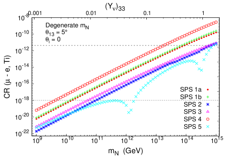
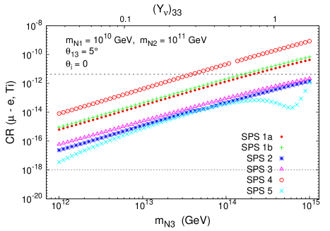
In Fig. 2, we display the prediction of CR(μe𝜇𝑒\mu-e, Ti) as a function of the heavy neutrino masses for the various SPS points, and for the particular choice θi=0subscript𝜃𝑖0\theta_{i}=0 (i=1,2,3𝑖123i=1,2,3) and θ13=5subscript𝜃13superscript5\theta_{13}=5^{\circ}. We also consider the case of degenerate and hierarchical heavy neutrino spectra (respectively left and right panels). In both scenarios for degenerate and hierarchical heavy neutrinos, we find a strong dependence on the the heavy neutrino masses. We also see that the rates for the various SPS points exhibit the following hierarchy, BR4 >> BR1b1b{}_{\text{1b}} greater-than-or-equivalent-to\gtrsim BR1a1a{}_{\text{1a}} >> BR3 greater-than-or-equivalent-to\gtrsim BR2 >> BR5. This behaviour can be understood in terms of the growth of the CRs with tanβ𝛽\tan\beta, and from the different mass spectra associated with each point.

In the case of degenerate heavy neutrinos, we find the expected fast growing behaviour of CR(μe𝜇𝑒\mu-e, Ti) as a function of the common neutrino mass mNsubscript𝑚𝑁m_{N}. For the values of mNsubscript𝑚𝑁m_{N} within the studied interval [109GeV,1015GeV]superscript109GeVsuperscript1015GeV\left[10^{9}\,\text{GeV},10^{15}\,\text{GeV}\right], the predictions for the CR(μe𝜇𝑒\mu-e, Ti) range over ten orders of magnitude. We also see that, for the chosen input parameter values, the predicted rates cross the experimental bound for the large mNsubscript𝑚𝑁m_{N} region. In the latter, the Yukawa couplings can be large (for instance, Y33νsuperscriptsubscript𝑌33𝜈Y_{33}^{\nu} and Y32νsuperscriptsubscript𝑌32𝜈Y_{32}^{\nu} can be 𝒪(1)𝒪1\mathcal{O}(1), while Y22νsuperscriptsubscript𝑌22𝜈Y_{22}^{\nu} and Y21νsuperscriptsubscript𝑌21𝜈Y_{21}^{\nu} can be of 𝒪(103)𝒪superscript103\mathcal{O}(10^{-3})), leading to excessively large rates, so that these large mNsubscript𝑚𝑁m_{N} values are disfavoured by data. The experimental bound is saturated for mNsubscript𝑚𝑁m_{N} values ranging from 2×10132superscript10132\times 10^{13} GeV for SPS 4 up to about 1015superscript101510^{15} GeV for SPS 5. In the case of hierarchical heavy neutrinos a similar behaviour of the predicted rates is found with respect to the heaviest neutrino mass, mN3subscript𝑚subscript𝑁3m_{N_{3}}. We have also checked that the conversion rates do not significantly depend on mN1subscript𝑚subscript𝑁1m_{N_{1}} and mN2subscript𝑚subscript𝑁2m_{N_{2}}, provided that their values are kept well below mN3subscript𝑚subscript𝑁3m_{N_{3}}. With the planned future sensitivity of 1018superscript101810^{-18} it will be possible to reach into wider regions of the heavy neutrino spectrum. Heavy neutrino masses above 1012superscript101210^{12} GeV can be probed for the several considered scenarios.

For most of the studied points, the previously illustrated dependence of the rates on the heavy neutrino masses is in agreement with the expected behaviour |mNlogmN|2superscriptsubscript𝑚𝑁subscript𝑚𝑁2~{}|m_{N}\log m_{N}|^{2} obtained in the LLog approximation (as derived from Eq. (4)). However, a clear departure from this approximation is found for some points, the most remarkable being the case of SPS 5. This failure of the LLog approximation has been known to happen in some scenarios, for instance those with either large A0subscript𝐴0A_{0}, or low M0subscript𝑀0M_{0} and large M1/2subscript𝑀12M_{1/2} [34].

Refer to caption Refer to caption
Figure 2: CR(μe𝜇𝑒\mu-e, Ti) as a function of the relevant heavy neutrino mass: mNsubscript𝑚𝑁m_{N} (on the left) and mN3subscript𝑚subscript𝑁3m_{N_{3}} (on the right), respectively associated with the degenerate and hierarchical cases. The predictions for SPS 1a (dots), 1b (crosses), 2 (asterisks), 3 (triangles), 4 (circles) and 5 (times) are included. On the upper horizontal axis we display the associated value of (Yν)33subscriptsubscript𝑌𝜈33(Y_{\nu})_{33}. In each case, we set θ13=5subscript𝜃13superscript5\theta_{13}=5^{\circ}, and consider the limit where R=1𝑅1R=1 (θi=0subscript𝜃𝑖0\theta_{i}=0). A dashed (dotted) horizontal line denotes the present experimental bound (future sensitivity).

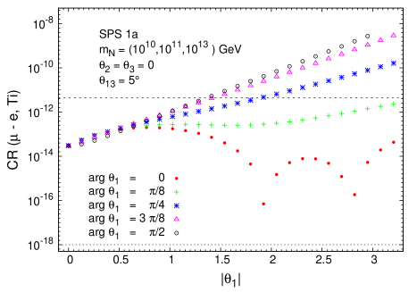
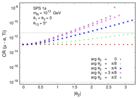
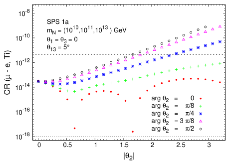
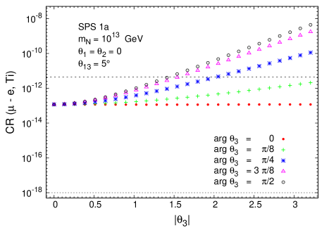
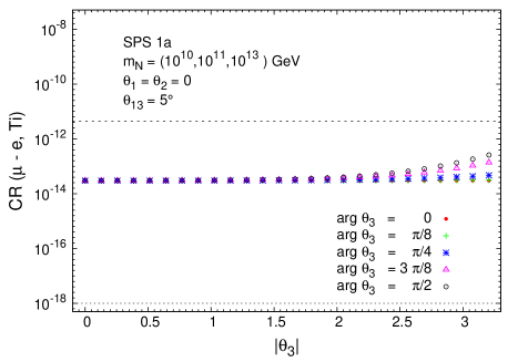
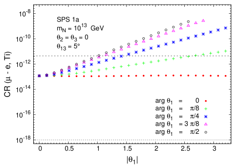
The predictions for CR(μe𝜇𝑒\mu-e, Ti) as a function of the R𝑅R-matrix angles, θ1,2,3subscript𝜃123\theta_{1,2,3}, are displayed in Fig. 3. In this case we have fixed the other relevant parameters as θ13=5subscript𝜃13superscript5\theta_{13}=5^{\circ}, mN=1013subscript𝑚𝑁superscript1013m_{N}=10^{13} GeV and mNi=(1010,1011,1013)subscript𝑚subscript𝑁𝑖superscript1010superscript1011superscript1013m_{N_{i}}=(10^{10},10^{11},10^{13}) GeV (degenerate and hierarchical heavy neutrinos, respectively) and chosen SPS 1a. To fully explore the variation of the rates with the complex angles111 Complex θisubscript𝜃𝑖\theta_{i} may imply the presence of CP violation in the neutrino Yukawa couplings. In addition to affecting the LFV rates, these phases will induce contributions to flavour-conserving CP violating observables, as is the case of charged lepton electric dipole moments (EDMs). Throughout the present study we have verified that the associated predictions for the charged lepton EDMs are in agreement with current experimental bounds [2]. θisubscript𝜃𝑖\theta_{i}, we have scanned the intervals 0<|θi|<π0subscript𝜃𝑖𝜋0<|\theta_{i}|<\pi rad and 0argθiπ20subscript𝜃𝑖𝜋20\leq\arg\theta_{i}\leq\frac{\pi}{2} rad. From this figure we see that the dependence on the three θisubscript𝜃𝑖\theta_{i} is very similar in the degenerate case, whereas the same does not occur for hierarchical heavy neutrinos. In the former, the rates smoothly grow with both modulus and argument, and are independent of θisubscript𝜃𝑖\theta_{i} in the real case. In the latter, the rates are almost independent of θ3subscript𝜃3\theta_{3}, and present a different minima pattern regarding θ1subscript𝜃1\theta_{1} and θ2subscript𝜃2\theta_{2}. The deep minima occuring in the real case are a consequence of the corresponding minima appearing in the relevant elements of the Yukawa couplings (as given by Eq. (9)). Notice that the observed behaviour of CR(μe𝜇𝑒\mu-e, Ti) as a function of θisubscript𝜃𝑖\theta_{i} can be indeed easily understood from the simple analytical expression obtained in the LLog approximation (cf. Eq. (4)).
Refer to caption Refer to caption
Figure 3: From top to bottom, CR(μe𝜇𝑒\mu-e, Ti) as a function of |θi|subscript𝜃𝑖|\theta_{i}| (i=1,2,3𝑖123i=1,2,3), for argθi={0,π/8,π/4, 3π/8,π/2}subscript𝜃𝑖0𝜋8𝜋43𝜋8𝜋2\arg\theta_{i}\,=\,\{0,\,\pi/8\,,\,\pi/4\,,\,3\pi/8,\,\pi/2\} (dots, crosses, asterisks, triangles and circles, respectively). Both |θi|subscript𝜃𝑖|\theta_{i}| and argθisubscript𝜃𝑖\arg{\theta_{i}} are given in radians. On the left we consider degenerate heavy neutrinos (with mN=1013subscript𝑚𝑁superscript1013m_{N}=10^{13} GeV), while on the right the hierarchical case is displayed (with mNi=(1010,1011,1013)subscript𝑚subscript𝑁𝑖superscript1010superscript1011superscript1013m_{N_{i}}=(10^{10},10^{11},10^{13}) GeV). In all cases we take θ13=5subscript𝜃13superscript5\theta_{13}=5^{\circ}, and set the CMSSM parameters to the SPS 1a case. A dashed (dotted) horizontal line denotes the present experimental bound (future sensitivity).

The most important outcome from Fig. 3 is that for both cases of degenerate and hierarchical heavy neutrinos, complex values of θisubscript𝜃𝑖\theta_{i} can increase the μe𝜇𝑒\mu-e conversion rates by almost five orders of magnitude with respect to the θi=0subscript𝜃𝑖0\theta_{i}=0 case. Only for a few specific choices of θisubscript𝜃𝑖\theta_{i} (for instance real θ1subscript𝜃1\theta_{1} or θ2subscript𝜃2\theta_{2}, in the hierarchical case) can we observe a strong decrease with respect to the θi=0subscript𝜃𝑖0\theta_{i}=0 case, but clearly this is not a generic situation.

In the following, and in order to simplify the analysis with respect to the other parameters, we will set θi=0subscript𝜃𝑖0\theta_{i}=0, and assume that the corresponding predictions for the CR(μe𝜇𝑒\mu-e, Ti) will constitute a representative case for the lowest conversion rates.
Refer to caption Refer to caption
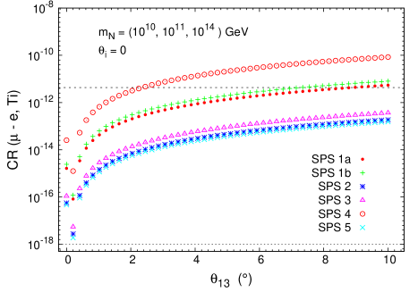
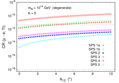
Figure 4: CR(μe𝜇𝑒\mu-e, Ti) as a function of θ13subscript𝜃13\theta_{13} (in degrees), for SPS 1a (dots), 1b (crosses), 2 (asterisks), 3 (triangles), 4 (circles) and 5 (times). On the left we consider degenerate heavy neutrinos (with mN=1014subscript𝑚𝑁superscript1014m_{N}=10^{14} GeV), while on the right the hierarchical case is displayed (with mNi=(1010,1011,1014)subscript𝑚subscript𝑁𝑖superscript1010superscript1011superscript1014m_{N_{i}}=(10^{10},10^{11},10^{14}) GeV). In both cases we choose R=1𝑅1R=1 (θi=0subscript𝜃𝑖0\theta_{i}=0). A dashed (dotted) horizontal line denotes the present experimental bound (future sensitivity).

In Fig. 4 we show the dependence of the μe𝜇𝑒\mu-e conversion rates on the light neutrino mixing angle θ13subscript𝜃13\theta_{13}. The other parameters are set to mN=1014subscript𝑚𝑁superscript1014m_{N}=10^{14} GeV, mNi=(1010,1011,1014)subscript𝑚subscript𝑁𝑖superscript1010superscript1011superscript1014m_{N_{i}}=(10^{10},10^{11},10^{14}) GeV, ( respectively for degenerate and hierarchical heavy neutrinos) and θi=0subscript𝜃𝑖0\theta_{i}=0. All the SPS points in Table 1 have been considered. For degenerate heavy neutrinos, the dependence on θ13subscript𝜃13\theta_{13} is softer than what is observed for the hierarchical case, leading to a variation in the rates of at most one order of magnitude in the studied range of 0θ1310superscript0subscript𝜃13superscript100^{\circ}\leq\theta_{13}\leq 10^{\circ} (the only exception being SPS 5, where the variation can reach up to two orders of magnitude). In contrast, this figure clearly manifests the very strong sensitivity of the CR(μe𝜇𝑒\mu-e, Ti) to the θ13subscript𝜃13\theta_{13} mixing angle for hierarchical heavy neutrinos. In the hierarchical case, a variation of θ13subscript𝜃13\theta_{13} in the studied interval leads to an increase in the conversion rates by as much as five orders of magnitude. This huge variation is due to the strong decrease of this observable for very small θ13subscript𝜃13\theta_{13} angles, as can be easily understood from the dependence on this angle of the dominant (L33mN3mν3c1c2s13)subscript𝐿33subscript𝑚subscript𝑁3subscript𝑚subscript𝜈3superscriptsubscript𝑐1superscriptsubscript𝑐2subscript𝑠13(L_{33}m_{N_{3}}\sqrt{m_{\nu_{3}}}c_{1}^{*}c_{2}^{*}s_{13}) term in Eq. (4). Furthermore, the minimum of CR(μe,Ti)𝜇𝑒Ti(\mu-e,\text{Ti}) is expected to occur at a vanishing mixing angle, but this being the value at the seesaw scale, i.e., θ13(mM)=0subscript𝜃13subscript𝑚𝑀0\theta_{13}(m_{M})=0. The deep minima in Fig. 4 are at θ13(mZ)0.2similar-to-or-equalssubscript𝜃13subscript𝑚𝑍superscript0.2\theta_{13}(m_{Z})\simeq 0.2^{\circ}, which is precisely the RGE shifted value at mZsubscript𝑚𝑍m_{Z} from θ13(mM)=0subscript𝜃13subscript𝑚𝑀0\theta_{13}(m_{M})=0. As θ13subscript𝜃13\theta_{13} grows, the predictions for SPS 4, SPS 1a and SPS 1b cross the present experimental bound. In particular, notice that for SPS 4, and for the present choice of input parameters, θ13subscript𝜃13\theta_{13} values larger than 2superscript22^{\circ} would be excluded by present data.

An equally remarkable sensitivity to θ13subscript𝜃13\theta_{13} has been found in other μe𝜇𝑒\mu-e violating processes, like μeγ𝜇𝑒𝛾\mu\to e\gamma and μ3e𝜇3𝑒\mu\to 3e, and also in tau decays as is the case of τeγ𝜏𝑒𝛾\tau\to e\gamma and τ3e𝜏3𝑒\tau\to 3e [34]. This interesting behaviour with θ13subscript𝜃13\theta_{13} has been proposed in [34] as a powerful tool to test the seesaw-I hypothesis for neutrino mass generation and, in case of a measurement of these branching ratios, as a unique way to derive some hints on the seesaw parameters, especially on the value of mN3subscript𝑚subscript𝑁3m_{N_{3}}. The μe𝜇𝑒\mu-e conversion rates here presented will certainly add new interesting information on this type of analysis. Fig. 4 also shows that with the expected future sensitivity of 1018superscript101810^{-18}, the full 0θ1310superscript0subscript𝜃13superscript100^{\circ}\leq\theta_{13}\leq 10^{\circ} interval can be thoroughly covered.

In the following study we will restrict ourselves to the hierarchical case where we have found this strong sensitivity to θ13subscript𝜃13\theta_{13}. For definiteness, we will also fix the heavy neutrino masses and θ13subscript𝜃13\theta_{13} to “reference” values of mNi=(1010,1011,1014)subscript𝑚subscript𝑁𝑖superscript1010superscript1011superscript1014m_{N_{i}}=(10^{10},10^{11},10^{14}) GeV and θ13=5subscript𝜃13superscript5\theta_{13}=5^{\circ}.

Refer to caption Refer to caption
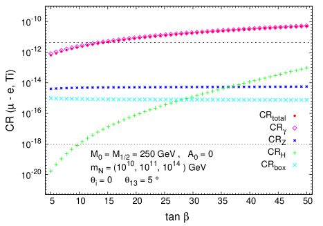
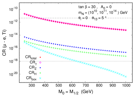
Figure 5: Contributions to CR(μe𝜇𝑒\mu-e, Ti): total (dots), γ𝛾\gamma-penguins (diamonds), Z𝑍Z-penguins (asterisks), H𝐻H-penguins (crosses) and box diagrams (times). On the left we present the dependence on tanβ𝛽\tan\beta, for M0=M1/2=250subscript𝑀0subscript𝑀12250M_{0}=M_{1/2}=250 GeV and A0=0subscript𝐴00A_{0}=0. On the right, we exhibit the evolution as a function of M0(=M1/2)annotatedsubscript𝑀0absentsubscript𝑀12M_{0}(=M_{1/2}), for tanβ=30𝛽30\tan\beta=30 and A0=0subscript𝐴00A_{0}=0. In either case, we consider hierarchical heavy neutrinos with mNi=(1010,1011,1014)subscript𝑚subscript𝑁𝑖superscript1010superscript1011superscript1014m_{N_{i}}=(10^{10},10^{11},10^{14}) GeV, and set θ13=5subscript𝜃13superscript5\theta_{13}=5^{\circ}, and R=1𝑅1R=1 (θi=0subscript𝜃𝑖0\theta_{i}=0). A dashed (dotted) horizontal line denotes the present experimental bound (future sensitivity).

Fig. 5 illustrates the predictions for the CR(μe𝜇𝑒\mu-e, Ti) as a function of tanβ𝛽\tan\beta, M0subscript𝑀0M_{0} and M1/2subscript𝑀12M_{1/2}. Here we have separately displayed the various contributions to the μe𝜇𝑒\mu-e conversion rates in order to conclude about their relative importance in this CMSSM-seesaw scenario. We set the values of the remaining CMSSM parameters to M0=M1/2=250subscript𝑀0subscript𝑀12250M_{0}=M_{1/2}=250 GeV in the study with tanβ𝛽\tan\beta (left panel) and to tanβ=30𝛽30\tan\beta=30 in the study with MSUSYM0=M1/2subscript𝑀SUSYsubscript𝑀0subscript𝑀12M_{\rm SUSY}\equiv M_{0}=M_{1/2} (right panel), taking A0=0subscript𝐴00A_{0}=0 in both cases. We choose our “reference” values of mN1,2,3=(1010,1011,1014)subscript𝑚subscript𝑁123superscript1010superscript1011superscript1014m_{N_{1,2,3}}=(10^{10},10^{11},10^{14}) GeV, θ13=5subscript𝜃13superscript5\theta_{13}=5^{\circ}, and θi=0subscript𝜃𝑖0\theta_{i}=0.

In both panels of Fig. 5 we clearly observe the dominance of the photon-mediated contributions, which are in fact indistinguishable from the total CR, for all the explored parameter ranges. The dependence of the various contributions on tanβ𝛽\tan\beta illustrates the expected fast growing behaviour with tan6βsuperscript6𝛽\tan^{6}\beta of the Higgs-mediated contributions, and the milder tan2βsuperscript2𝛽\tan^{2}\beta dependence of the photon-mediated ones. In addition, we see that the Z𝑍Z boson-mediated and the box diagram contributions are almost independent of tanβ𝛽\tan\beta. Although not displayed in this plot, we have also verified that the Higgs-mediated contribution is largely dominated by the exchange of H0superscript𝐻0H^{0}, which is indeed the Higgs boson with enhanced couplings to charged leptons in the large tanβ𝛽\tan\beta regime.

The decoupling behaviour for large MSUSYsubscript𝑀SUSYM_{\rm SUSY} of each of these contributions (CRγsubscriptCR𝛾{\rm CR}_{\gamma}, CRZsubscriptCR𝑍{\rm CR}_{Z}, CRHsubscriptCR𝐻{\rm CR}_{H} and CRboxsubscriptCRbox{\rm CR}_{\rm box}) is clearly manifested in the right panel of Fig. 5. The most important conclusion from this figure is that, within a CMSSM-seesaw scenario, the γ𝛾\gamma-penguin diagrams completely dominate the conversion rates, even for the largest tanβ𝛽\tan\beta considered (tanβ=𝛽absent\tan\beta=50). Therefore, the total CR(μe𝜇𝑒\mu-e, Ti) does not manifest the Higgs contributions, so that in this universal scenario there is no chance for the μe𝜇𝑒\mu-e conversion process to provide any information on the Higgs sector. We will see next that the situation is remarkably different in the non-universal case, where the Higgs contributions turn out to be much larger than in the universal case.

4.2 Non-universality: NUHM-seesaw

The numerical results for the NUHM-seesaw scenario are collected in figures 6 through 11.

In order to study the influence of the hypothesis of non-universal Higgs soft SUSY breaking masses, MH1,2subscript𝑀subscript𝐻12M_{H_{1,2}}, on the μe𝜇𝑒\mu-e conversion rates, we have first explored the impact of the non-universality parameters δ1subscript𝛿1\delta_{1} and δ2subscript𝛿2\delta_{2} on the predicted Higgs boson masses. The values for these parameters have been taken to lie within the interval 2δ1,222subscript𝛿122-2\leq\delta_{1,2}\leq 2.

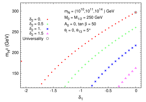
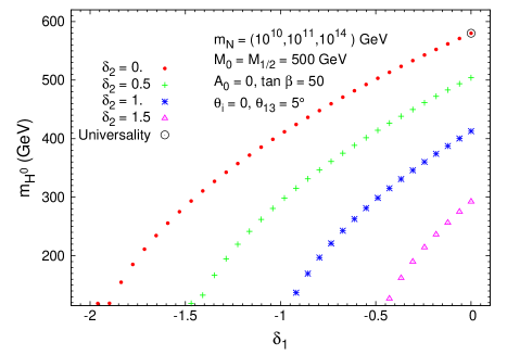
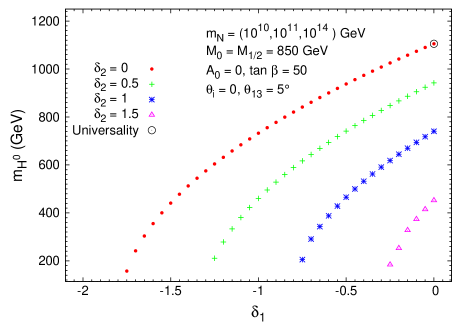
The predictions for the relevant Higgs boson mass, mH0subscript𝑚superscript𝐻0m_{H^{0}}, as a function of δ1subscript𝛿1\delta_{1} and δ2subscript𝛿2\delta_{2} are summarised in Fig. 6. We have chosen here the largest value of tanβ=50𝛽50\tan\beta=50 and three representative values of MSUSY=subscript𝑀SUSYabsentM_{\rm SUSY}= 250, 500 and 850 GeV for moderate, heavy and very heavy SUSY spectra, respectively. The other parameters are set to our “reference” values of mNi=(1010,1011,1014)subscript𝑚subscript𝑁𝑖superscript1010superscript1011superscript1014m_{N_{i}}=(10^{10},10^{11},10^{14}) GeV, θi=0subscript𝜃𝑖0\theta_{i}=0, A0=0subscript𝐴00A_{0}=0, θ13=5subscript𝜃13superscript5\theta_{13}=5^{\circ} and sign(μ)=+1sign𝜇1{\rm sign}(\mu)=+1.

Refer to caption Refer to caption
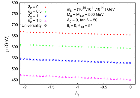
Figure 6: Mass of the heaviest Higgs scalar (mH0subscript𝑚superscript𝐻0m_{H^{0}}) as a function of the non-universality parameter δ1subscript𝛿1\delta_{1}, for fixed values of δ2={0, 0.5, 1, 1.5}subscript𝛿200.511.5\delta_{2}=\{0,\,0.5,\,1,\,1.5\} (respectively dots, crosses, asterisks, triangles). The universality case δ1,2=0subscript𝛿120\delta_{1,2}=0 is represented by a large circle. We also take mNi=(1010,1011,1014)subscript𝑚subscript𝑁𝑖superscript1010superscript1011superscript1014m_{N_{i}}=(10^{10},10^{11},10^{14}) GeV, set θi=0subscript𝜃𝑖0\theta_{i}=0, A0=0subscript𝐴00A_{0}=0, tanβ=50𝛽50\tan\beta=50 and impose the relation M0=M1/2subscript𝑀0subscript𝑀12M_{0}=M_{1/2}. The first three plots correspond to M0=250, 500subscript𝑀0250500M_{0}=250,\,500 and 850 GeV, respectively. On the fourth plot, we display the μ𝜇\mu parameter as a function of the non-universality parameter δ1subscript𝛿1\delta_{1}, for fixed values of δ2subscript𝛿2\delta_{2}, and for M0=M1/2=500subscript𝑀0subscript𝑀12500M_{0}=M_{1/2}=500 GeV.

First, it is important to mention that not all the considered values of the δ1,2subscript𝛿12\delta_{1,2} parameters and MSUSYsubscript𝑀SUSYM_{\rm SUSY} allow for a correct SU(2)×U(1)𝑆𝑈2𝑈1SU(2)\times U(1) breaking. In fact some particular choices for δ1subscript𝛿1\delta_{1}, δ2subscript𝛿2\delta_{2}, and MSUSYsubscript𝑀SUSYM_{\rm SUSY} lead to unacceptable negative values of Bμ𝐵𝜇B\mu (and hence, negative mA02subscriptsuperscript𝑚2superscript𝐴0m^{2}_{A^{0}}). For instance, this is the case when δ1,2subscript𝛿12\delta_{1,2} are simultaneously positive or negative. Some other points, despite leading to a proper SU(2)×U(1)𝑆𝑈2𝑈1SU(2)\times U(1) breaking, are nevertheless not acceptable, since they lead to a Higgs boson sector which is too light, with masses below the present experimental lower limits. To ensure that our results are indeed experimentally viable, we have included in this, and in the following figures, only the solutions where the three neutral Higgs boson masses are above the experimental bound for the lightest MSSM Higgs boson, which at present is 110 GeV for tanβ>5𝛽5\tan{\beta}>5 (99.7%percent99.799.7\% C.L.) [2]. The most interesting solutions with important phenomenological implications are found for negative δ1subscript𝛿1\delta_{1} and positive δ2subscript𝛿2\delta_{2}, the choice selected for Fig. 6. In this figure, for all the explored values of δ1subscript𝛿1\delta_{1} and δ2subscript𝛿2\delta_{2}, we find a value of mH0subscript𝑚superscript𝐻0m_{H^{0}} that is significantly smaller than what one would encounter in the universal case (here represented by the choice δ1=δ2=0subscript𝛿1subscript𝛿20\delta_{1}=\delta_{2}=0). This is truly remarkable in the case of large soft breaking masses, as can be seen, for instance, in the panel with MSUSY=850subscript𝑀SUSY850M_{\rm SUSY}=850 GeV, where low values of mH0subscript𝑚superscript𝐻0m_{H^{0}} are still found, even close to the experimental limit. For completeness we have also shown in Fig. 6 the predictions for the μ𝜇\mu parameter as a function of δ1subscript𝛿1\delta_{1} and δ2subscript𝛿2\delta_{2}. This parameter turns out to be nearly independent of δ1subscript𝛿1\delta_{1}, and its largest values are obtained for δ2=0subscript𝛿20\delta_{2}=0.

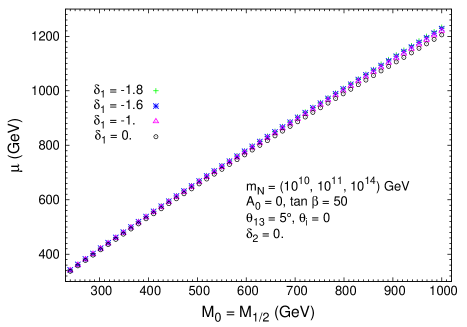
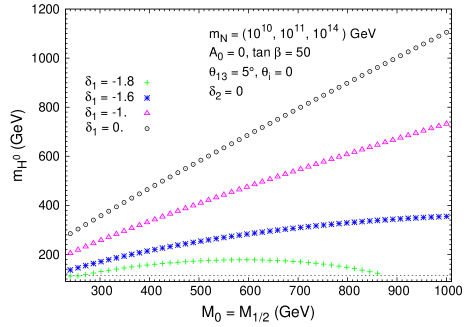
The behaviour of the predicted mH0subscript𝑚superscript𝐻0m_{H^{0}} and μ𝜇\mu parameter as a function of MSUSY=M0=M1/2subscript𝑀SUSYsubscript𝑀0subscript𝑀12M_{\rm SUSY}=M_{0}=M_{1/2} is shown in Fig. 7. Here the specific values of δ1={1.8,1.6,1, 0}subscript𝛿11.81.61 0\delta_{1}=\{-1.8,\,-1.6,\,-1,\,0\} and δ2=0subscript𝛿20\delta_{2}=0 have been considered. This figure again illustrates the interesting departure from the linear behaviour of mH0subscript𝑚superscript𝐻0m_{H^{0}} with MSUSYsubscript𝑀SUSYM_{\rm SUSY}, which is generic in the universal case (δ1,2=0subscript𝛿120\delta_{1,2}=0). In contrast, the μ𝜇\mu parameter conserves a similar linear behaviour with MSUSYsubscript𝑀SUSYM_{\rm SUSY} in all the studied scenarios (universal and non-universal).
Refer to caption Refer to caption
Figure 7: On the left, mass of the heaviest Higgs scalar (mH0subscript𝑚superscript𝐻0m_{H^{0}}) as a function of the SUSY scale (MSUSY=M0=M1/2subscript𝑀SUSYsubscript𝑀0subscript𝑀12M_{\text{SUSY}}=M_{0}=M_{1/2}), for fixed values of δ1={1.8,1.6,1, 0}subscript𝛿11.81.61 0\delta_{1}=\{-1.8,\,-1.6,\,-1,\,0\} (respectively crosses, asterisks, triangles and circles). We take mNi=(1010,1011,1014)subscript𝑚subscript𝑁𝑖superscript1010superscript1011superscript1014m_{N_{i}}=(10^{10},10^{11},10^{14}) GeV, and set θi=0subscript𝜃𝑖0\theta_{i}=0, A0=0subscript𝐴00A_{0}=0, tanβ=50𝛽50\tan\beta=50 with θ13=5subscript𝜃13superscript5\theta_{13}=5^{\circ}. On the right, the μ𝜇\mu-parameter is displayed as a function of MSUSYsubscript𝑀SUSYM_{\text{SUSY}}, for the same choices of SUSY-seesaw parameters.

As a representative example of these interesting non-universal points, we explicitly refer to the case with δ1=1.8subscript𝛿11.8\delta_{1}=-1.8 and δ2=0subscript𝛿20\delta_{2}=0, where the predicted masses are mH0=subscript𝑚superscript𝐻0absentm_{H^{0}}= 113, 174 and 127 GeV for MSUSY=subscript𝑀SUSYabsentM_{\rm SUSY}= 250, 500 and 850 GeV, respectively. For completeness, we have also collected the corresponding masses of the other relevant SUSY particles in Table 2. Notice that, in the case of MSUSY=subscript𝑀SUSYabsentM_{\rm SUSY}= 850 GeV, this table illustrates a very heavy SUSY spectrum, even with a considerably heavy lightest SUSY particle, mχ~10=362subscript𝑚superscriptsubscript~𝜒10362m_{\tilde{\chi}_{1}^{0}}=362 GeV, but where the relevant Higgs boson is still light, mH0=127subscript𝑚superscript𝐻0127m_{H^{0}}=127 GeV.

MSSM masses MSUSYsubscript𝑀SUSY{M_{\rm SUSY}} (GeV)
(GeV) 250 500 850
ml~1subscript𝑚subscript~𝑙1m_{\tilde{l}_{1}} 175 415 734
ml~2subscript𝑚subscript~𝑙2m_{\tilde{l}_{2}} 258 511 867
ml~3subscript𝑚subscript~𝑙3m_{\tilde{l}_{3}} 258 511 867
ml~4subscript𝑚subscript~𝑙4m_{\tilde{l}_{4}} 307 594 985
ml~5subscript𝑚subscript~𝑙5m_{\tilde{l}_{5}} 309 607 1025
ml~6subscript𝑚subscript~𝑙6m_{\tilde{l}_{6}} 323 609 1031
mν~1subscript𝑚subscript~𝜈1m_{\tilde{\nu}_{1}} 281 571 971
mν~2subscript𝑚subscript~𝜈2m_{\tilde{\nu}_{2}} 297 601 1022
mν~3subscript𝑚subscript~𝜈3m_{\tilde{\nu}_{3}} 299 605 1028
mχ~1subscript𝑚superscriptsubscript~𝜒1m_{\tilde{\chi}_{1}^{-}} 185 395 687
mχ~2subscript𝑚superscriptsubscript~𝜒2m_{\tilde{\chi}_{2}^{-}} 379 679 1075
mχ~10subscript𝑚superscriptsubscript~𝜒10m_{\tilde{\chi}_{1}^{0}} 99 207 362
mχ~20subscript𝑚superscriptsubscript~𝜒20m_{\tilde{\chi}_{2}^{0}} 185 394 687
mχ~30subscript𝑚superscriptsubscript~𝜒30m_{\tilde{\chi}_{3}^{0}} 363 668 1067
mχ~40subscript𝑚superscriptsubscript~𝜒40m_{\tilde{\chi}_{4}^{0}} 377 678 1074
mh0subscript𝑚superscript0m_{h^{0}} 110 119 123
mH0subscript𝑚superscript𝐻0m_{H^{0}} 113 174 127
Table 2: Relevant MSSM spectra for M0=M1/2=MSUSYsubscript𝑀0subscript𝑀12subscript𝑀SUSYM_{0}=M_{1/2}=M_{\rm SUSY}, tanβ=50𝛽50\tan{\beta}=50, A0=0subscript𝐴00A_{0}=0, θi=0subscript𝜃𝑖0\theta_{i}=0, θ13=5subscript𝜃13superscript5\theta_{13}=5^{\circ}, MNi=(1010,1011,1014)subscript𝑀subscript𝑁𝑖superscript1010superscript1011superscript1014M_{N_{i}}=(10^{10},10^{11},10^{14}) GeV, δ1=1.8subscript𝛿11.8\delta_{1}=-1.8 and δ2=0subscript𝛿20\delta_{2}=0.

In the following we present the predictions of the μe𝜇𝑒\mu-e conversion rates in Titanium nuclei within the NUHM-seeesaw scenario. First we display in Fig. 8 the CR(μe,Ti)𝜇𝑒Ti(\mu-e,\text{Ti}) as a function of M0=M1/2=MSUSYsubscript𝑀0subscript𝑀12subscript𝑀SUSYM_{0}=M_{1/2}=M_{\text{SUSY}} and of A0subscript𝐴0A_{0} for the particular choice δ1=1.8subscript𝛿11.8\delta_{1}=-1.8 and δ2=0subscript𝛿20\delta_{2}=0. In order to illustrate the impact of the non-universality hypothesis on the conversion rates, we have separately displayed in this plot the various contributions from the γ𝛾\gamma-, Z𝑍Z-, Higgs mediated penguins and box diagrams. We observe a very distinct behaviour with MSUSYsubscript𝑀SUSYM_{\text{SUSY}} of the Higgs-mediated contributions when compared to what was found for the CMSSM (universal) case, shown in Fig. 5. In fact, for the choice of input parameters in this plot, the Higgs-mediated contribution can equal, or even exceed that of the photon, dominating the total conversion rate in the large MSUSYsubscript𝑀SUSYM_{\text{SUSY}} region. Both photon- and Higgs-mediated contributions are similar around MSUSY=700subscript𝑀SUSY700M_{\text{SUSY}}=700 GeV. These larger Higgs contributions are the obvious consequence of the lighter Higgs boson mass values encountered in this region, as previously illustrated in Figs. 6 and 7. The non-decoupling behaviour of the SUSY particles for the large MSUSYsubscript𝑀SUSYM_{\text{SUSY}} regime can be seen in the Higgs contribution, and thus in the total rates for the Higgs-dominated case.

For completeness, we have also explored other choices of A0subscript𝐴0A_{0} and sign(μ)𝜇(\mu). The case of sign(μ)=1𝜇1(\mu)=-1, whose numerical results are not presented here, does not evidence any interesting new feature. In fact, there is a much more reduced δ1subscript𝛿1\delta_{1}, δ2subscript𝛿2\delta_{2} parameter space allowing for the correct SU(2)×U(1)𝑆𝑈2𝑈1SU(2)\times U(1) breaking. In addition, for sign(μ)=1𝜇1(\mu)=-1 we have not found solutions displaying as small values of mH0subscript𝑚superscript𝐻0m_{H^{0}} as in the case of sign(μ)=+1𝜇1(\mu)=+1. The predicted Higgs contributions to the conversion rates are correspondingly smaller, and therefore less interesting. Regarding A0subscript𝐴0A_{0}, the right panel in Fig. 8 shows that all the contributions are essentially independent of the value of the universal trilinear coupling, so that our selected value, A0=0subscript𝐴00A_{0}=0, is in fact a good representative point.
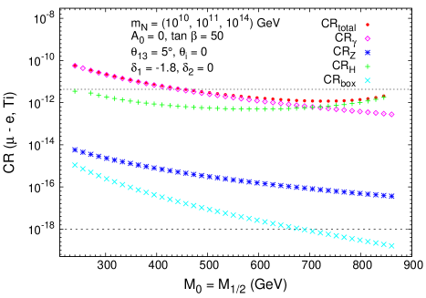
Refer to caption Refer to caption
Figure 8: Contributions to CR(μe𝜇𝑒\mu-e, Ti) as a function of M0(=M1/2)annotatedsubscript𝑀0absentsubscript𝑀12M_{0}(=M_{1/2}) (left) and A0subscript𝐴0A_{0} (right): total (dots), γ𝛾\gamma-penguins ( diamonds), Z𝑍Z-penguins (asterisks), H𝐻H-penguins (crosses) and box diagrams (times), for δ1=1.8subscript𝛿11.8\delta_{1}=-1.8 and δ2=0subscript𝛿20\delta_{2}=0. We set tanβ=50𝛽50\tan\beta=50 and take θ13=5subscript𝜃13superscript5\theta_{13}=5^{\circ}, R=1𝑅1R=1 (θi=0subscript𝜃𝑖0\theta_{i}=0) and mNi=(1010,1011,1014)subscript𝑚subscript𝑁𝑖superscript1010superscript1011superscript1014m_{N_{i}}=(10^{10},10^{11},10^{14}) GeV. On the left A0=0subscript𝐴00A_{0}=0, while on the right we choose M0(=M1/2)=700annotatedsubscript𝑀0absentsubscript𝑀12700M_{0}(=M_{1/2})=700 GeV. In each case, a dashed (dotted) horizontal line denotes the present experimental bound (future sensitivity).

Within the NUHM-seesaw scenario, we have also studied the μe𝜇𝑒\mu-e conversion rates for other nuclei. The case of Gold is particularly interesting since its present experimental bound of 7×10137superscript10137\times 10^{-13} [10] is more stringent than the present bound for Titanium (4.3×10124.3superscript10124.3\times 10^{-12} [9]). In Fig. 9 we display the predicted μe𝜇𝑒\mu-e conversion rates for Al, Ti, Sr, Sb, Au and Pb, as a function of MSUSYsubscript𝑀SUSYM_{\text{SUSY}}. We have chosen two light, two moderate and two heavy nuclei and we have fixed the other parameters to those of the previously elected non-universality reference point (with δ1=1.8subscript𝛿11.8\delta_{1}=-1.8 and δ2=0subscript𝛿20\delta_{2}=0). For completeness, the values of the relevant parameters for these nuclei, Zeffsubscript𝑍effZ_{\rm eff}, Fpsubscript𝐹𝑝F_{p} and ΓcapturesubscriptΓcapture\Gamma_{\rm capture}, have been collected in Table 3 and follow [35]. In this figure we clearly see that throughout most of the explored MSUSYsubscript𝑀SUSYM_{\text{SUSY}} interval, the relative conversion rates obey the hierarchy CR(μe𝜇𝑒\mu-e, Sb) >> CR(μe𝜇𝑒\mu-e, Sr) >> CR(μe𝜇𝑒\mu-e, Ti) >> CR(μe𝜇𝑒\mu-e, Au) >> CR(μe𝜇𝑒\mu-e, Pb) >> CR(μe𝜇𝑒\mu-e, Al), in agreement with the generic results in [35]. We do not find a significant difference in the large MSUSYsubscript𝑀SUSYM_{\rm SUSY} region, where the Higgs-contribution dominates the ratios. The predicted rates for Ti, Au and Pb tend to converge whereas the corresponding curve for Al nuclei deviates slightly from the others at large MSUSYsubscript𝑀SUSYM_{\text{SUSY}}, but we do not consider these differences among the predictions for the various nuclei to be relevant. The most important conclusion from Fig. 9 concerns the fact that we have found predictions for Gold nuclei which, for the input parameters in this plot, are clearly above its present experimental bound throughout the explored MSUSYsubscript𝑀SUSYM_{\text{SUSY}} interval. However, it should be recalled that the formulae here used for these estimates come from approximations that may not properly work for the case of very heavy nuclei. These heavy nuclei deserve a more dedicated and refined study.
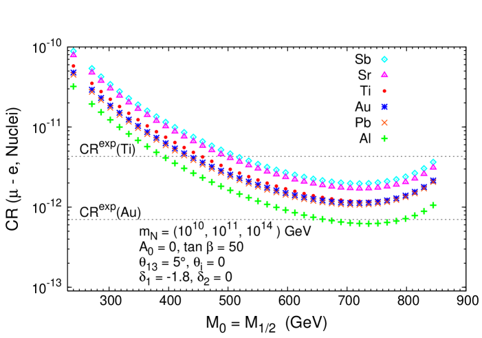
Refer to caption
Figure 9: μe𝜇𝑒\mu-e conversion rates for various nuclei as a function of M0=M1/2subscript𝑀0subscript𝑀12M_{0}=M_{1/2} in the NUHM-seesaw. We display the theoretical predictions for Sb, Sr, Ti, Au, Pb and Al nuclei (diamonds, triangles, dots, asterisks, times and crosses, respectively). We have taken mNi=(1010,1011,1014)subscript𝑚subscript𝑁𝑖superscript1010superscript1011superscript1014m_{N_{i}}=(10^{10},10^{11},10^{14}) GeV, A0=0subscript𝐴00A_{0}=0, tanβ=50𝛽50\tan\beta=50, θ13=5subscript𝜃13superscript5\theta_{13}=5^{\circ} and R=1𝑅1R=1 (θi=0subscript𝜃𝑖0\theta_{i}=0). The non-universality parameters are set to δ1=1.8subscript𝛿11.8\delta_{1}=-1.8 and δ2=0subscript𝛿20\delta_{2}=0. From top to bottom, the horizontal dashed lines denote the present experimental bounds for CR(μe𝜇𝑒\mu-e, Ti) and CR(μe𝜇𝑒\mu-e, Au).

Before proceeding with our analysis, let us briefly mention that for the region investigated in Fig. 9, the SUSY contributions to the anomalous magnetic moment of the muon, aμ=(gμ2)subscript𝑎𝜇subscript𝑔𝜇2a_{\mu}=(g_{\mu}-2), range from aμSUSY=108superscriptsubscript𝑎𝜇SUSYsuperscript108a_{\mu}^{\text{SUSY}}=10^{-8} for MSUSY=250subscript𝑀SUSY250M_{\text{SUSY}}=250 GeV to aμSUSY=109superscriptsubscript𝑎𝜇SUSYsuperscript109a_{\mu}^{\text{SUSY}}=10^{-9}, in association with MSUSY=850subscript𝑀SUSY850M_{\text{SUSY}}=850 GeV. The latter values are in fair agreement with the observed excess in aμexpsuperscriptsubscript𝑎𝜇expa_{\mu}^{\text{exp}} when compared to the SM prediction, which, at the 3.8 σ𝜎\sigma is given by aμSUSY=aμexpaμSM=3.32×10⁹superscriptsubscript𝑎𝜇SUSYsuperscriptsubscript𝑎𝜇expsuperscriptsubscript𝑎𝜇SM3.32superscript109a_{\mu}^{\text{SUSY}}=a_{\mu}^{\text{exp}}-a_{\mu}^{\text{SM}}=3.32\times 10^{-9} at 3.8σ3.8𝜎3.8\sigma (for a review, see for instance [36] and references therein).

AZsuperscriptsubscriptabsent𝑍𝐴{}_{Z}^{A}Nucleus Zeffsubscript𝑍effZ_{\rm eff} Fpsubscript𝐹𝑝F_{p} Γcapt(GeV)subscriptΓcaptGeV\Gamma_{\rm capt}{\rm(GeV)}
2713superscriptsubscriptabsent1327{}_{13}^{27}Al 11.5 0.64 4.64079×10194.64079superscript10194.64079\times 10^{-19}
4822superscriptsubscriptabsent2248{}_{22}^{48}Ti 17.6 0.54 1.70422×10181.70422superscript10181.70422\times 10^{-18}
8038superscriptsubscriptabsent3880{}_{38}^{80}Sr 25.0 0.39 4.61842×10184.61842superscript10184.61842\times 10^{-18}
12151superscriptsubscriptabsent51121{}_{51}^{121}Sb 29.0 0.32 6.71711×10186.71711superscript10186.71711\times 10^{-18}
19779superscriptsubscriptabsent79197{}_{79}^{197}Au 33.5 0.16 8.59868×10188.59868superscript10188.59868\times 10^{-18}
20782superscriptsubscriptabsent82207{}_{82}^{207}Pb 34.0 0.15 8.84868×10188.84868superscript10188.84868\times 10^{-18}
Table 3: Values of Zeffsubscript𝑍effZ_{\rm eff}, Fpsubscript𝐹𝑝F_{p} and ΓcaptsubscriptΓcapt\Gamma_{\rm capt} for different nuclei, as taken from [35].

To complete our study of the μe𝜇𝑒\mu-e conversion rates in the NUHM-seesaw scenario we have compared the theoretical predictions for the CR(μe𝜇𝑒\mu-e, Ti) with those for the BR(μeγ𝜇𝑒𝛾\mu\to e\gamma). We recall that both observables are sensitive to the same leptonic mixing given by the slepton mass matrix entries connecting the first and the second generation. In the usual photon-penguin dominated case, the latter two quantities are known to be highly correlated, and this is indeed what occurred for the CMSSM-seesaw discussed in Sec. 4.1. In other seesaw scenarios, as for instance, SUSY-GUT seesaw [37] or the inverse seesaw [38], this strong correlation still persists. However, for some scenarios where the photon-mediated diagrams are no longer the dominant contributions to the conversion rates, the strong correlation between CR(μe,Ti)𝜇𝑒Ti(\mu-e,\text{Ti}) and BR(μeγ)𝜇𝑒𝛾(\mu\to e\gamma) can be lost. For instance, this loss of correlation has been found in the case of Littlest Higgs Models, as recently pointed out in [39].

We have also found an interesting loss of correlation in the present case of the NUHM-scenario, where, as previously discussed, the Higgs-contributions can be the dominant ones. The departure from the strongly correlated regime for (CR(μe𝜇𝑒\mu-e, Ti), BR(μeγ𝜇𝑒𝛾\mu\to e\gamma)) is illustrated in Fig. 10, considering several choices of the neutrino mixing angle θ13=10,5,1,0.2subscript𝜃13superscript10superscript5superscript1superscript0.2\theta_{13}=10^{\circ},5^{\circ},1^{\circ},0.2^{\circ}. For all plots the predictions for (CR(μe𝜇𝑒\mu-e, Ti), BR(μeγ𝜇𝑒𝛾\mu\to e\gamma)) have been derived for several choices of the non-universality parameter δ1subscript𝛿1\delta_{1}, scanning over the following interval 250 GeVMSUSY1000 GeV250 GeVsubscript𝑀SUSY1000 GeV250\text{ GeV}\leq M_{\text{SUSY}}\leq 1000\text{ GeV}. In each of the panels, the predictions for (CR(μe𝜇𝑒\mu-e, Ti), BR(μeγ𝜇𝑒𝛾\mu\to e\gamma)) that correspond to δ1=δ2=0subscript𝛿1subscript𝛿20\delta_{1}=\delta_{2}=0 fall upon a straight line, which strongly supports the correlated behaviour of the two observables in this case. As MSUSYsubscript𝑀SUSYM_{\text{SUSY}} increases within the considered interval, (CR(μe𝜇𝑒\mu-e, Ti), BR(μeγ𝜇𝑒𝛾\mu\to e\gamma)) moves left and downwards along the straight line due to the obvious decrease of the rate with MSUSYsubscript𝑀SUSYM_{\text{SUSY}}.

However a clear departure from the previous strongly correlated predictions is found for other values of δ1subscript𝛿1\delta_{1}, δ2subscript𝛿2\delta_{2}. In particular, for the specific δ1subscript𝛿1\delta_{1} and δ2subscript𝛿2\delta_{2} values where, as previously shown, the Higgs contributions dominate the μe𝜇𝑒\mu-e conversion rates, the predicted (CR(μe𝜇𝑒\mu-e, Ti), BR(μeγ𝜇𝑒𝛾\mu\to e\gamma)) points exhibit a different behaviour, deviating from the straight line associated with the universal case. The separation between the correlated and uncorrelated regimes is maximal for the δ1=1.8subscript𝛿11.8\delta_{1}=-1.8, δ2=0subscript𝛿20\delta_{2}=0 non-universal case, as can be clearly understood from our previous results. We find this loss of correlation a very promising phenomenon that could be fully explored if future sensitivities of 1018superscript101810^{-18} are reached.

Secondly, it is clear from Fig. 10 that even in the most pessimistic situation of very small θ13subscript𝜃13\theta_{13}, the theoretical predictions for CR(μe𝜇𝑒\mu-e, Ti), and in particular the corresponding curved line, are well above the horizontal line at 1018superscript101810^{-18}. This is quite a challenging possibility, since for those high values of MSUSY850similar-tosubscript𝑀SUSY850M_{\text{SUSY}}\sim 850 GeV, whose predictions lie at the left end of the curved and straight lines, the predicted BR(μeγ𝜇𝑒𝛾\mu\to e\gamma) is far below the planned 1013superscript101310^{-13} sensitivity. This clearly reflects that μe𝜇𝑒\mu-e in nuclei can be a very competitive process to study LFV within the SUSY seesaw.
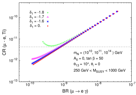
Refer to caption Refer to caption
Figure 10: CR(μe𝜇𝑒\mu-e, Ti) versus BR(μeγ𝜇𝑒𝛾\mu\to e\gamma) for 250 GeVMSUSY1000 GeV250 GeVsubscript𝑀SUSY1000 GeV250\text{ GeV}\leq M_{\text{SUSY}}\leq 1000\text{ GeV}, and δ1=1.8,1.7,1.6, 0subscript𝛿11.81.71.6 0\delta_{1}=-1.8,\,-1.7,\,-1.6,\,0 (crosses, triangles, asterisks, dots, respectively). We set δ2=0subscript𝛿20\delta_{2}=0, and take mNi=(1010,1011,1014)subscript𝑚subscript𝑁𝑖superscript1010superscript1011superscript1014m_{N_{i}}=(10^{10},10^{11},10^{14}) GeV, A0=0subscript𝐴00A_{0}=0, tanβ=50𝛽50\tan\beta=50 and R=1𝑅1R=1 (θi=0subscript𝜃𝑖0\theta_{i}=0). From left to right and top to bottom, the panels are associated with θ13=10,5,1subscript𝜃13superscript10superscript5superscript1\theta_{13}=10^{\circ},5^{\circ},1^{\circ} and 0.2superscript0.20.2^{\circ}. In each case, the horizontal and vertical dashed (dotted) lines denote the present experimental bounds (future sensitivities) for CR(μe𝜇𝑒\mu-e, Ti) and BR(μeγ𝜇𝑒𝛾\mu\to e\gamma), respectively.
Refer to caption
Figure 11: Ratio CR(μe𝜇𝑒\mu-e, Ti)/BR(μeγ𝜇𝑒𝛾\mu\to e\gamma) as a function of the Higgs mass, mH0subscript𝑚superscript𝐻0m_{H^{0}}. We take mNi=(1010,1011,1014)subscript𝑚subscript𝑁𝑖superscript1010superscript1011superscript1014m_{N_{i}}=(10^{10},10^{11},10^{14}) GeV, A0=0subscript𝐴00A_{0}=0, tanβ=50𝛽50\tan\beta=50, θ13=5subscript𝜃13superscript5\theta_{13}=5^{\circ} and R=1𝑅1R=1 (θi=0subscript𝜃𝑖0\theta_{i}=0), and scan over 250 GeV \leq MSUSYsubscript𝑀SUSYM_{\rm SUSY} \leq 1000 GeV, 2δ102subscript𝛿10-2\leq\delta_{1}\leq 0, and 0δ220subscript𝛿220\leq\delta_{2}\leq 2 (grey dots). We have highlighted specific choices of δ2=0, 0.1, 0.2, 1.1subscript𝛿200.10.21.1\delta_{2}=0,\,0.1,\,0.2,\,1.1 (crosses, triangles, diamonds, dots, respectively). In each tilted cluster, we have also indicated the values of δ1subscript𝛿1\delta_{1} associated with the δ2subscript𝛿2\delta_{2} coloured points. The universality limit (δ1=δ2=0subscript𝛿1subscript𝛿20\delta_{1}=\delta_{2}=0) is denoted by a circle. Asterisks denote points with MSUSY=876subscript𝑀SUSY876M_{\text{SUSY}}=876 GeV and δ2=0.1subscript𝛿20.1\delta_{2}=0.1.

Finally, and to summarise the most striking results for these NUHM-seesaw scenarios, we plot in Fig. 11 the ratio of the two predicted rates, CR(μe𝜇𝑒\mu-e, Ti)/BR(μeγ𝜇𝑒𝛾\mu\to e\gamma) as a function of mH0subscript𝑚superscript𝐻0m_{H^{0}}. Since both observables exhibit the same dependence on mNisubscript𝑚subscript𝑁𝑖m_{N_{i}}, θisubscript𝜃𝑖\theta_{i} and θ13subscript𝜃13\theta_{13}, the consideration of this ratio of rates allows to reduce the number of relevant parameters to tanβ𝛽\tan\beta, MSUSYsubscript𝑀SUSYM_{\rm SUSY} and δ1,2subscript𝛿12\delta_{1,2}. These last two are clearly the leading ones given that they drive the solutions to the interesting low mH0subscript𝑚superscript𝐻0m_{H^{0}} values. In this figure, and in order to maximise the Higgs-contribution to the total μe𝜇𝑒\mu-e conversion rates we have again considered the extreme tanβ=50𝛽50\tan\beta=50 value. For consistency, we have set the remaining parameters to their reference values, but as we have said, they will not play a relevant role in this study.

Leading to this scatter plot, we have scanned in the intervals 2<δ1<02subscript𝛿10-2<\delta_{1}<0, 0<δ2<20subscript𝛿220<\delta_{2}<2 and 250 GeV << MSUSYsubscript𝑀SUSYM_{\rm SUSY} << 1000 GeV. The most important conclusion from this plot is that the ratio CR(μe𝜇𝑒\mu-e, Ti)/BR(μeγ𝜇𝑒𝛾\mu\to e\gamma) can deviate from the constant prediction of 5×1035superscript1035\times 10^{-3} of the universality case by as much as a factor of almost 10. For the scan here conducted, the maximum value of this ratio of rates is found for δ1=1.7subscript𝛿11.7\delta_{1}=-1.7, δ2=0.1subscript𝛿20.1\delta_{2}=0.1 and MSUSY=876subscript𝑀SUSY876M_{\text{SUSY}}=876 GeV, and its size is 0.04.

Considering larger values of MSUSYsubscript𝑀SUSYM_{\text{SUSY}} and identical intervals for δ1,2subscript𝛿12\delta_{1,2} leads to somewhat similar results: one finds the same pattern of clusters departing from the constant value of the universal case, but the maximum value of CR(μe𝜇𝑒\mu-e, Ti)/BR(μeγ𝜇𝑒𝛾\mu\to e\gamma) is in general smaller than the 0.04 obtained in the scan of Fig. 11. The reason why this ratio is not improved at larger values of MSUSYsubscript𝑀SUSYM_{\text{SUSY}} than 1 TeV is because the acceptable solutions producing the proper SU(2)×U(1)𝑆𝑈2𝑈1SU(2)\times U(1) breaking do not lead to sufficiently light Higgs bosons.

Even without the knowledge of the seesaw parameters, a measurement of CR(μe𝜇𝑒\mu-e, Ti) and BR(μeγ𝜇𝑒𝛾\mu\to e\gamma), together with information on tanβ𝛽\tan{\beta} and the SUSY scale, may allow to shed some light into the Higgs sector.

5 Conclusions

In this work we have extensively studied the lepton flavour violating process of μe𝜇𝑒\mu-e conversion in nuclei, within the context of the SUSY-seesaw. In particular, we considered two distinct scenarios, the CMSSM-seesaw, and the NUHM-seesaw, obtained by partially relaxing the universality conditions of the Higgs boson masses. Throughout our analysis, we compared our theoretical predictions with the present experimental bounds, and with the challenging future sensitivities. In fact, the latter may convert processes like CR(μe𝜇𝑒\mu-e, Ti) into one of the most sensitive probes to new physics.

We have presented here the first full one-loop computation of the μe𝜇𝑒\mu-e conversion in nuclei, including the complete set of SUSY-loop diagrams: γ𝛾\gamma-mediated, Z𝑍Z- and Higgs-boson mediated penguins and box diagrams. We have also provided the full analytical results working in terms of physical eigenstates (for all intervening SUSY and Higgs particles).

For the CMSSM-seesaw, we have considered the dependence of the conversion rates on the several parameters defining the scenario. Choosing the well known SPS benchmark points to specify the CMSSM parameters, we focused on the most relevant parameters in the neutrino sector, namely on the heavy neutrino masses (mNisubscript𝑚subscript𝑁𝑖m_{N_{i}}), the complex θisubscript𝜃𝑖\theta_{i} mixing angles and the still undetermined angle of the UMNSsubscript𝑈MNSU_{\text{MNS}} matrix, θ13subscript𝜃13\theta_{13}. As discussed here, the CRs exhibit a very pronounced dependence on the previous parameters, with variations that can reach up to ten orders of magnitude in the case of mNisubscript𝑚subscript𝑁𝑖m_{N_{i}} and up to five orders of magnitude in the cases of θisubscript𝜃𝑖\theta_{i} and θ13subscript𝜃13\theta_{13}, for the investigated ranges. In turn, this strong dependence implies that a comparison of the theoretical predictions with the present experimental bound allows to derive indirect upper bounds for the unknown seesaw parameters.

We have pointed out that the highest sensitivity is found for the case of hierarchical heavy neutrinos. In this case, the conversion rates are essentially dependent on mN3subscript𝑚subscript𝑁3m_{N_{3}} and θ1,2subscript𝜃12\theta_{1,2}, manifesting an extreme sensitivity to θ13subscript𝜃13\theta_{13} (for the case of vanishing θisubscript𝜃𝑖\theta_{i}). In fact, the values of these parameters in the upper part of their studied intervals, 1012GeVmN31015GeVsuperscript1012GeVsubscript𝑚subscript𝑁3superscript1015GeV10^{12}\,{\rm GeV}\leq m_{N_{3}}\leq 10^{15}\,{\rm GeV}, 0|θ1,2|<π0subscript𝜃12𝜋0\leq|\theta_{1,2}|<\pi, 0arg(θ1,2)π/20argsubscript𝜃12𝜋20\leq{\rm arg}(\theta_{1,2})\leq\pi/2 and 0θ1310superscript0subscript𝜃13superscript100^{\circ}\leq\theta_{13}\leq 10^{\circ} are already in conflict with the present upper bounds on CR(μe𝜇𝑒\mu-e, Ti) and CR(μe𝜇𝑒\mu-e, Au).

We have put special emphasis on the sensitivity of the CR(μe𝜇𝑒\mu-e,Ti) to θ13subscript𝜃13\theta_{13}, given that either a measurement, or a more stringent bound on this parameter is expected in the near future [40]. Therefore, and once θ13subscript𝜃13\theta_{13} is measured, a dedicated study of the μe𝜇𝑒\mu-e conversion rates could provide some insight into the potentially unreachable heavy neutrino parameters.

In all the studied examples of the CMSSM-seesaw, the dominant contribution to the μe𝜇𝑒\mu-e conversion rates clearly arises from the photon-penguins. Even though we have verified that the Higgs contributions do indeed grow with tan6βsuperscript6𝛽\tan^{6}\beta, they induce contributions which are several orders of magnitude below those of the photon (which grow as tan2βsuperscript2𝛽\tan^{2}\beta) for all the studied interval 5tanβ505𝛽505\leq\tan\beta\leq 50. A very interesting departure from this situation occurs when one relaxes the universality condition for the Higgs soft breaking masses, and this fuelled our interest to consider the NUHM-seesaw.

In the case of the NUHM-seesaw, we explored the influence of the non-universality hypothesis of the soft SUSY breaking masses MH1,2subscript𝑀subscript𝐻12M_{H_{1,2}} on the μe𝜇𝑒\mu-e conversion rates. The δ1subscript𝛿1\delta_{1} and δ2subscript𝛿2\delta_{2} parameters that describe the departure from universality in the Higgs sector have an important impact on the predicted Higgs boson masses. In particular, we have found regimes for δ1,2subscript𝛿12\delta_{1,2} with very interesting phenomenological implications, namely the possibility of a light Higgs spectrum, even in the limit of large soft SUSY masses. As a concrete example, we recall that for the reference choice of δ1=1.8subscript𝛿11.8\delta_{1}=-1.8, δ2=0subscript𝛿20\delta_{2}=0, we find mH0=subscript𝑚superscript𝐻0absentm_{H^{0}}= 113, 174 and 127 GeV for MSUSY=250,500,850subscript𝑀SUSY250500850M_{\rm SUSY}=250,500,850 GeV respectively (in turn associated with moderate, heavy and very heavy sparticle spectra).

The distinctive NUHM-seesaw scenarios associated with light H0superscript𝐻0H^{0} bosons and a relatively heavy SUSY spectra induce very interesting and unique predictions for the μe𝜇𝑒\mu-e conversion rates. Specifically, we have shown that in the large MSUSY=M0=M1/2subscript𝑀SUSYsubscript𝑀0subscript𝑀12M_{\rm SUSY}=M_{0}=M_{1/2} region (e.g. above 700 GeV), there is a strong enhancement in the Higgs-dominated rates, leading to a remarkable loss of correlation between the CRs in nuclei and the BRs of μeγ𝜇𝑒𝛾\mu\to e\gamma decays. As we aimed at illustrating in Fig. 10, the departure from the linear correlation of these two observables can be sizable. It is worth stressing that if both these rates and θ13subscript𝜃13\theta_{13} are measured, values of BR(μeγ𝜇𝑒𝛾\mu\to e\gamma) and CR(μe𝜇𝑒\mu-e, Ti) that clearly deviate from the expected SUSY-seesaw ratio in the photon-dominated case, can provide indirect information into the structure of the Higgs sector.

It is also important to remark that with the expected future sensitivities, μe𝜇𝑒\mu-e conversion in nuclei maybe sensitive to LFV signals that lie beyond the reach of the future sensitivities to μeγ𝜇𝑒𝛾\mu\to e\gamma decays. For example, this can occur for a heavy SUSY spectrum, and very small values of θ13subscript𝜃13\theta_{13}.

Finally, we considered the predictions for the ratio CR(μe𝜇𝑒\mu-e, Ti)/BR(μeγ𝜇𝑒𝛾\mu\to e\gamma) as a a function of mH0subscript𝑚superscript𝐻0m_{H^{0}} in NUHM-seesaw scenarios, comparing the results with those obtained for the CMSSM-seesaw case. The most important conclusion to be drawn from this study (which is presented in Fig. 11) is that in the NUHM-seesaw one can observe a clear deviation from the constant prediction of the CMSSM-seesaw by as much as a factor close to 10. If such deviation is indeed observed, we can obtain some indirect hints regarding the SUSY Higgs sector.

In summary, with the expected future sensitivities, μe𝜇𝑒\mu-e conversion in nuclei can clearly be more competitive for the study of LFV in SUSY-seesaw than μeγ𝜇𝑒𝛾\mu\to e\gamma, and certainly provide an important tool for the study of the Higgs sector.

Acknowledgements

We acknowledge S. Antusch for his participation in the initial stages of this work. We are grateful to S. Ritt for providing important information on the experimental status of present bounds and future sensitivities of LFV muon decays and μe𝜇𝑒\mu-e conversion rates in nuclei. We are also indebted to D.G. Cerdeño for valuable discussions on the NUHM scenarios. E. Arganda acknowledges the Spanish MEC for financial support under the grant AP2003-3776. The work of A. M. Teixeira has been supported by the French ANR project PHYS@COL&COS. This work was partially supported by the Spanish MEC under project FPA2006-05423 and by the regional “Comunidad de Madrid” HEPHACOS project.

Appendix A One-loop formulae for μe𝜇𝑒\mu-e conversion in nuclei

In this appendix we collect all the analytical results of the SUSY one-loop diagrams that contribute to the μe𝜇𝑒\mu-e conversion rates in nuclei. These are summarised by the photon-, Z𝑍Z-boson- and Higgs-boson- penguins and box diagrams in Figs. 121314 and 15, respectively. In the following subsections we present the relevant formulae for each separate contribution. All the loop functions in the formulae are taken from [33, 41].

A.1 Form factors for the γμe𝛾𝜇𝑒\gamma\mu e vertex

Refer to caption
Figure 12: Relevant SUSY one-loop diagrams for the photon-mediated contributions to μe𝜇𝑒\mu-e conversion in nuclei.

Our convention for the form factors A1,2L,Rsuperscriptsubscript𝐴12𝐿𝑅A_{1,2}^{L,R} defining the γμe𝛾𝜇𝑒\gamma\mu e vertex is as follows:

ie[q2γα(A1LPL+A1RPR)+imμσαβqβ(AaLPL+A2RPR)],𝑖𝑒delimited-[]superscript𝑞2subscript𝛾𝛼superscriptsubscript𝐴1𝐿subscript𝑃𝐿superscriptsubscript𝐴1𝑅subscript𝑃𝑅𝑖subscript𝑚𝜇subscript𝜎𝛼𝛽superscript𝑞𝛽superscriptsubscript𝐴𝑎𝐿subscript𝑃𝐿superscriptsubscript𝐴2𝑅subscript𝑃𝑅ie\left[q^{2}\gamma_{\alpha}(A_{1}^{L}P_{L}+A_{1}^{R}P_{R})+im_{\mu}\sigma_{\alpha\beta}q^{\beta}(A_{a}^{L}P_{L}+A_{2}^{R}P_{R})\right], (35)

where q𝑞q is the off-shell photon momentum, PL,R=(1γ5)/2subscript𝑃𝐿𝑅minus-or-plus1subscript𝛾52P_{L,R}=(1\mp\gamma_{5})/2, e𝑒e is the electromagnetic charge and mμsubscript𝑚𝜇m_{\mu} is the muon mass.

In the SUSY-seesaw context there are one-loop contributions to these form factors that come from the chargino and neutralino sectors respectively,

AaL,R=Aa(n)L.R+Aa(c)L,R,a=1,2.formulae-sequencesuperscriptsubscript𝐴𝑎𝐿𝑅superscriptsubscript𝐴𝑎formulae-sequence𝑛𝐿𝑅superscriptsubscript𝐴𝑎𝑐𝐿𝑅𝑎12A_{a}^{L,R}=A_{a}^{(n)L.R}+A_{a}^{(c)L,R},\quad a=1,2\,. (36)

The neutralino contributions are given by,

A1(n)Lsuperscriptsubscript𝐴1𝑛𝐿\displaystyle A_{1}^{(n)L} =\displaystyle= 1576π2NeAXRNμAXR1ml~X229xAX+18xAX211xAX3+6xAX3logxAX(1xAX)41576superscript𝜋2superscriptsubscript𝑁𝑒𝐴𝑋𝑅superscriptsubscript𝑁𝜇𝐴𝑋𝑅1superscriptsubscript𝑚subscript~𝑙𝑋229subscript𝑥𝐴𝑋18superscriptsubscript𝑥𝐴𝑋211superscriptsubscript𝑥𝐴𝑋36superscriptsubscript𝑥𝐴𝑋3subscript𝑥𝐴𝑋superscript1subscript𝑥𝐴𝑋4\displaystyle\frac{1}{576\pi^{2}}N_{eAX}^{R}N_{\mu AX}^{R\ast}\frac{1}{m_{\tilde{l}_{X}}^{2}}\frac{2-9x_{AX}+18x_{AX}^{2}-11x_{AX}^{3}+6x_{AX}^{3}\log{x_{AX}}}{\left(1-x_{AX}\right)^{4}}
A2(n)Lsuperscriptsubscript𝐴2𝑛𝐿\displaystyle A_{2}^{(n)L} =\displaystyle= 132π21ml~X2[NeAXLNμAXL16xAX+3xAX2+2xAX36xAX2logxAX6(1xAX)4\displaystyle\frac{1}{32\pi^{2}}\frac{1}{m_{\tilde{l}_{X}}^{2}}\left[N_{eAX}^{L}N_{\mu AX}^{L\ast}\frac{1-6x_{AX}+3x_{AX}^{2}+2x_{AX}^{3}-6x_{AX}^{2}\log{x_{AX}}}{6\left(1-x_{AX}\right)^{4}}\right. (38)
+\displaystyle+ NeAXRNμAXRmemμ16xAX+3xAX2+2xAX36xAX2logxAX6(1xAX)4superscriptsubscript𝑁𝑒𝐴𝑋𝑅superscriptsubscript𝑁𝜇𝐴𝑋𝑅subscript𝑚𝑒subscript𝑚𝜇16subscript𝑥𝐴𝑋3superscriptsubscript𝑥𝐴𝑋22superscriptsubscript𝑥𝐴𝑋36superscriptsubscript𝑥𝐴𝑋2subscript𝑥𝐴𝑋6superscript1subscript𝑥𝐴𝑋4\displaystyle N_{eAX}^{R}N_{\mu AX}^{R\ast}\frac{m_{e}}{m_{\mu}}\frac{1-6x_{AX}+3x_{AX}^{2}+2x_{AX}^{3}-6x_{AX}^{2}\log{x_{AX}}}{6\left(1-x_{AX}\right)^{4}}
+\displaystyle+ NeAXLNμAXRmχ~A0mμ1xAX2+2xAXlogxAX(1xAX)3],\displaystyle\left.N_{eAX}^{L}N_{\mu AX}^{R\ast}\frac{m_{\tilde{\chi}_{A}^{0}}}{m_{\mu}}\frac{1-x_{AX}^{2}+2x_{AX}\log{x_{AX}}}{\left(1-x_{AX}\right)^{3}}\right],
Aa(n)Rsuperscriptsubscript𝐴𝑎𝑛𝑅\displaystyle A_{a}^{(n)R} =\displaystyle= Aa(n)L|LR,evaluated-atsuperscriptsubscript𝐴𝑎𝑛𝐿𝐿𝑅\displaystyle\left.A_{a}^{(n)L}\right|_{L\leftrightarrow R}, (39)

where xAX=mχ~A02/ml~X2subscript𝑥𝐴𝑋superscriptsubscript𝑚superscriptsubscript~𝜒𝐴02superscriptsubscript𝑚subscript~𝑙𝑋2x_{AX}=m_{\tilde{\chi}_{A}^{0}}^{2}/m_{\tilde{l}_{X}}^{2} and the indices are A=1,..,4A=1,..,4, X=1,..,6X=1,..,6.

The chargino contributions are given by

A1(c)Lsuperscriptsubscript𝐴1𝑐𝐿\displaystyle A_{1}^{(c)L} =\displaystyle= 1576π2CeAXRCμAXR1mν~X21645xAX+36xAX27xAX3+6(23xAX)logxAX(1xAX)4,1576superscript𝜋2superscriptsubscript𝐶𝑒𝐴𝑋𝑅superscriptsubscript𝐶𝜇𝐴𝑋𝑅1superscriptsubscript𝑚subscript~𝜈𝑋21645subscript𝑥𝐴𝑋36superscriptsubscript𝑥𝐴𝑋27superscriptsubscript𝑥𝐴𝑋3623subscript𝑥𝐴𝑋subscript𝑥𝐴𝑋superscript1subscript𝑥𝐴𝑋4\displaystyle-\frac{1}{576\pi^{2}}C_{eAX}^{R}C_{\mu AX}^{R\ast}\frac{1}{m_{\tilde{\nu}_{X}}^{2}}\frac{16-45x_{AX}+36x_{AX}^{2}-7x_{AX}^{3}+6(2-3x_{AX})\log{x_{AX}}}{\left(1-x_{AX}\right)^{4}},
A2(c)Lsuperscriptsubscript𝐴2𝑐𝐿\displaystyle A_{2}^{(c)L} =\displaystyle= 132π21mν~X2[CeAXLCμAXL2+3xAX6xAX2+xAX3+6xAXlogxAX6(1xAX)4\displaystyle-\frac{1}{32\pi^{2}}\frac{1}{m_{\tilde{\nu}_{X}}^{2}}\left[C_{eAX}^{L}C_{\mu AX}^{L\ast}\frac{2+3x_{AX}-6x_{AX}^{2}+x_{AX}^{3}+6x_{AX}\log{x_{AX}}}{6\left(1-x_{AX}\right)^{4}}\right. (42)
+\displaystyle+ CeAXRCμAXRmemμ2+3xAX6xAX2+xAX3+6xAXlogxAX6(1xAX)4superscriptsubscript𝐶𝑒𝐴𝑋𝑅superscriptsubscript𝐶𝜇𝐴𝑋𝑅subscript𝑚𝑒subscript𝑚𝜇23subscript𝑥𝐴𝑋6superscriptsubscript𝑥𝐴𝑋2superscriptsubscript𝑥𝐴𝑋36subscript𝑥𝐴𝑋subscript𝑥𝐴𝑋6superscript1subscript𝑥𝐴𝑋4\displaystyle C_{eAX}^{R}C_{\mu AX}^{R\ast}\frac{m_{e}}{m_{\mu}}\frac{2+3x_{AX}-6x_{AX}^{2}+x_{AX}^{3}+6x_{AX}\log{x_{AX}}}{6\left(1-x_{AX}\right)^{4}}
+\displaystyle+ CeAXLCμAXRmχ~Amμ3+4xAXxAX22logxAX(1xAX)3],\displaystyle\left.C_{eAX}^{L}C_{\mu AX}^{R\ast}\frac{m_{\tilde{\chi}_{A}^{-}}}{m_{\mu}}\frac{-3+4x_{AX}-x_{AX}^{2}-2\log{x_{AX}}}{\left(1-x_{AX}\right)^{3}}\right],
Aa(c)Rsuperscriptsubscript𝐴𝑎𝑐𝑅\displaystyle A_{a}^{(c)R} =\displaystyle= Aa(c)L|LR,evaluated-atsuperscriptsubscript𝐴𝑎𝑐𝐿𝐿𝑅\displaystyle\left.A_{a}^{(c)L}\right|_{L\leftrightarrow R}, (43)

where in this case xAX=mχ~A2/mν~X2subscript𝑥𝐴𝑋superscriptsubscript𝑚superscriptsubscript~𝜒𝐴2superscriptsubscript𝑚subscript~𝜈𝑋2x_{AX}=m_{\tilde{\chi}_{A}^{-}}^{2}/m_{\tilde{\nu}_{X}}^{2} and the indices are A=1,2𝐴12A=1,2, X=1,2,3𝑋123X=1,2,3. Notice that in both neutralino and chargino contributions a summation over the indices A𝐴A and X𝑋X is understood.

A.2 Form factors for the Zμe𝑍𝜇𝑒Z\mu e vertex

Our convention for the form factors FL,Rsubscript𝐹𝐿𝑅F_{L,R} defining the Zμe𝑍𝜇𝑒Z\mu e vertex is as follows:

iγμ[FLPL+FRPR].𝑖subscript𝛾𝜇delimited-[]subscript𝐹𝐿subscript𝑃𝐿subscript𝐹𝑅subscript𝑃𝑅-i\gamma_{\mu}\left[F_{L}P_{L}+F_{R}P_{R}\right]. (44)
Refer to caption
Figure 13: Relevant SUSY one-loop diagrams for the Z𝑍Z-mediated contributions to μe𝜇𝑒\mu-e conversion in nuclei

The Z𝑍Z-boson form factors have also the two kinds of contributions, from neutralinos (n)𝑛(n) and charginos (c)𝑐(c),

FL(R)=FL(R)(n)+FL(R)(c).subscript𝐹𝐿𝑅superscriptsubscript𝐹𝐿𝑅𝑛superscriptsubscript𝐹𝐿𝑅𝑐F_{L(R)}=F_{L(R)}^{(n)}+F_{L(R)}^{(c)}\,. (45)

The results for the corresponding form factors are the following:

FL(n)superscriptsubscript𝐹𝐿𝑛\displaystyle F_{L}^{(n)} =\displaystyle= 116π2{NeBXRNμAXR[2EBAR(n)C24(ml~X2,mχ~A02,mχ~B02)EBAL(n)mχ~A0mχ~B0C0(ml~X2,mχ~A02,mχ~B02)]\displaystyle-\frac{1}{16\pi^{2}}\left\{N_{eBX}^{R}N_{\mu AX}^{R\ast}\left[2E_{BA}^{R(n)}C_{24}(m_{\tilde{l}_{X}}^{2},m_{\tilde{\chi}_{A}^{0}}^{2},m_{\tilde{\chi}_{B}^{0}}^{2})-E_{BA}^{L(n)}m_{\tilde{\chi}_{A}^{0}}m_{\tilde{\chi}_{B}^{0}}C_{0}(m_{\tilde{l}_{X}}^{2},m_{\tilde{\chi}_{A}^{0}}^{2},m_{\tilde{\chi}_{B}^{0}}^{2})\right]\right. (46)
+\displaystyle+ NeAXRNμAYR[2QXYl~C24(mχ~A02,ml~X2,ml~Y2)]+NeAXRNμAXR[ZL(l)B1(mχ~A02,ml~X2)]},\displaystyle\left.N_{eAX}^{R}N_{\mu AY}^{R\ast}\left[2Q_{XY}^{\tilde{l}}C_{24}(m_{\tilde{\chi}_{A}^{0}}^{2},m_{\tilde{l}_{X}}^{2},m_{\tilde{l}_{Y}}^{2})\right]+N_{eAX}^{R}N_{\mu AX}^{R\ast}\left[Z_{L}^{(l)}B_{1}(m_{\tilde{\chi}_{A}^{0}}^{2},m_{\tilde{l}_{X}}^{2})\right]\right\},
FR(n)superscriptsubscript𝐹𝑅𝑛\displaystyle F_{R}^{(n)} =\displaystyle= FL(n)|LR,evaluated-atsuperscriptsubscript𝐹𝐿𝑛𝐿𝑅\displaystyle\left.F_{L}^{(n)}\right|_{L\leftrightarrow R}, (47)
FL(c)superscriptsubscript𝐹𝐿𝑐\displaystyle F_{L}^{(c)} =\displaystyle= 116π2{CeBXRCμAXR[2EBAR(c)C24(mν~X2,mχ~A2,mχ~B2)EBAL(c)mχ~Amχ~BC0(mν~X2,mχ~A2,mχ~B2)]\displaystyle-\frac{1}{16\pi^{2}}\left\{C_{eBX}^{R}C_{\mu AX}^{R\ast}\left[2E_{BA}^{R(c)}C_{24}(m_{\tilde{\nu}_{X}}^{2},m_{\tilde{\chi}_{A}^{-}}^{2},m_{\tilde{\chi}_{B}^{-}}^{2})-E_{BA}^{L(c)}m_{\tilde{\chi}_{A}^{-}}m_{\tilde{\chi}_{B}^{-}}C_{0}(m_{\tilde{\nu}_{X}}^{2},m_{\tilde{\chi}_{A}^{-}}^{2},m_{\tilde{\chi}_{B}^{-}}^{2})\right]\right. (48)
+\displaystyle+ CeAXRCμAYR[2QXYν~C24(mχ~A2,mν~X2,mν~Y2)]+CeAXRCμAXR[ZL(l)B1(mχ~A2,mν~X2)]},\displaystyle\left.C_{eAX}^{R}C_{\mu AY}^{R\ast}\left[2Q_{XY}^{\tilde{\nu}}C_{24}(m_{\tilde{\chi}_{A}^{-}}^{2},m_{\tilde{\nu}_{X}}^{2},m_{\tilde{\nu}_{Y}}^{2})\right]+C_{eAX}^{R}C_{\mu AX}^{R\ast}\left[Z_{L}^{(l)}B_{1}(m_{\tilde{\chi}_{A}^{-}}^{2},m_{\tilde{\nu}_{X}}^{2})\right]\right\},
FR(c)superscriptsubscript𝐹𝑅𝑐\displaystyle F_{R}^{(c)} =\displaystyle= FL(c)|LR,evaluated-atsuperscriptsubscript𝐹𝐿𝑐𝐿𝑅\displaystyle\left.F_{L}^{(c)}\right|_{L\leftrightarrow R}, (49)

where again the indices are A,B=1,..,4A,B=1,..,4, X,Y=1,..,6X,Y=1,..,6 in the contributions from the neutralino sector and A,B=1,2formulae-sequence𝐴𝐵12A,B=1,2, X,Y=1,2,3formulae-sequence𝑋𝑌123X,Y=1,2,3 in the contributions from the chargino sector, and a summation over the various indices is understood.

A.3 Form factors for the Hμe𝐻𝜇𝑒H\mu e vertex

Our convention for the form factors HL,Rsubscript𝐻𝐿𝑅H_{L,R} defining the Hμe𝐻𝜇𝑒H\mu e vertex is as follows:

iγμ[HLPL+HRPR].𝑖subscript𝛾𝜇delimited-[]subscript𝐻𝐿subscript𝑃𝐿subscript𝐻𝑅subscript𝑃𝑅i\gamma_{\mu}\left[H_{L}P_{L}+H_{R}P_{R}\right]. (50)
Refer to caption
Figure 14: Relevant SUSY one-loop diagrams for the Higgs-mediated contributions to μe𝜇𝑒\mu-e conversion in nuclei.

As in the previous cases, we separate the contributions from the neutralino and chargino sectors,

HL(R)=HL(R),n(p)+HL(R),c(p).subscript𝐻𝐿𝑅superscriptsubscript𝐻𝐿𝑅𝑛𝑝superscriptsubscript𝐻𝐿𝑅𝑐𝑝H_{L(R)}=H_{L(R),n}^{(p)}+H_{L(R),c}^{(p)}. (51)

The results for the form factors are the following,

HL,n(p)superscriptsubscript𝐻𝐿𝑛𝑝\displaystyle H_{L,n}^{(p)} =\displaystyle= 116π2{[B0(mχ~A02,mχ~B02)+ml~X2C0(ml~X2,mχ~A02,mχ~B02)+mμ2C12(ml~X2,mχ~A02,mχ~B02)\displaystyle-\frac{1}{16\pi^{2}}\left\{\left[B_{0}(m_{\tilde{\chi}_{A}^{0}}^{2},m_{\tilde{\chi}_{B}^{0}}^{2})+m_{\tilde{l}_{X}}^{2}C_{0}(m_{\tilde{l}_{X}}^{2},m_{\tilde{\chi}_{A}^{0}}^{2},m_{\tilde{\chi}_{B}^{0}}^{2})+m_{\mu}^{2}C_{12}(m_{\tilde{l}_{X}}^{2},m_{\tilde{\chi}_{A}^{0}}^{2},m_{\tilde{\chi}_{B}^{0}}^{2})\right.\right. (52)
+\displaystyle+ me2(C11C12)(ml~X2,mχ~A02,mχ~B02)]NeAXLDR,AB(p)NμBXR\displaystyle\left.m_{e}^{2}(C_{11}-C_{12})(m_{\tilde{l}_{X}}^{2},m_{\tilde{\chi}_{A}^{0}}^{2},m_{\tilde{\chi}_{B}^{0}}^{2})\right]N_{eAX}^{L}D_{R,AB}^{(p)}N_{\mu BX}^{R\ast}
+\displaystyle+ memμ(C11+C0)(ml~X2,mχ~A02,mχ~B02)NeAXRDL,AB(p)NμBXLsubscript𝑚𝑒subscript𝑚𝜇subscript𝐶11subscript𝐶0superscriptsubscript𝑚subscript~𝑙𝑋2superscriptsubscript𝑚superscriptsubscript~𝜒𝐴02superscriptsubscript𝑚superscriptsubscript~𝜒𝐵02superscriptsubscript𝑁𝑒𝐴𝑋𝑅superscriptsubscript𝐷𝐿𝐴𝐵𝑝superscriptsubscript𝑁𝜇𝐵𝑋𝐿\displaystyle m_{e}m_{\mu}(C_{11}+C_{0})(m_{\tilde{l}_{X}}^{2},m_{\tilde{\chi}_{A}^{0}}^{2},m_{\tilde{\chi}_{B}^{0}}^{2})N_{eAX}^{R}D_{L,AB}^{(p)}N_{\mu BX}^{L\ast}
+\displaystyle+ memχ~B0(C11C12+C0)(ml~X2,mχ~A02,mχ~B02)NeAXRDL,AB(p)NμBXRsubscript𝑚𝑒subscript𝑚superscriptsubscript~𝜒𝐵0subscript𝐶11subscript𝐶12subscript𝐶0superscriptsubscript𝑚subscript~𝑙𝑋2superscriptsubscript𝑚superscriptsubscript~𝜒𝐴02superscriptsubscript𝑚superscriptsubscript~𝜒𝐵02superscriptsubscript𝑁𝑒𝐴𝑋𝑅superscriptsubscript𝐷𝐿𝐴𝐵𝑝superscriptsubscript𝑁𝜇𝐵𝑋𝑅\displaystyle m_{e}m_{\tilde{\chi}_{B}^{0}}(C_{11}-C_{12}+C_{0})(m_{\tilde{l}_{X}}^{2},m_{\tilde{\chi}_{A}^{0}}^{2},m_{\tilde{\chi}_{B}^{0}}^{2})N_{eAX}^{R}D_{L,AB}^{(p)}N_{\mu BX}^{R\ast}
+\displaystyle+ mμmχ~B0C12(ml~X2,mχ~A02,mχ~B02)NeAXLDR,AB(p)NμBXLsubscript𝑚𝜇subscript𝑚superscriptsubscript~𝜒𝐵0subscript𝐶12superscriptsubscript𝑚subscript~𝑙𝑋2superscriptsubscript𝑚superscriptsubscript~𝜒𝐴02superscriptsubscript𝑚superscriptsubscript~𝜒𝐵02superscriptsubscript𝑁𝑒𝐴𝑋𝐿superscriptsubscript𝐷𝑅𝐴𝐵𝑝superscriptsubscript𝑁𝜇𝐵𝑋𝐿\displaystyle m_{\mu}m_{\tilde{\chi}_{B}^{0}}C_{12}(m_{\tilde{l}_{X}}^{2},m_{\tilde{\chi}_{A}^{0}}^{2},m_{\tilde{\chi}_{B}^{0}}^{2})N_{eAX}^{L}D_{R,AB}^{(p)}N_{\mu BX}^{L\ast}
+\displaystyle+ memχ~A0(C11C12)(ml~X2,mχ~A02,mχ~B02)NeAXRDR,AB(p)NμBXRsubscript𝑚𝑒subscript𝑚superscriptsubscript~𝜒𝐴0subscript𝐶11subscript𝐶12superscriptsubscript𝑚subscript~𝑙𝑋2superscriptsubscript𝑚superscriptsubscript~𝜒𝐴02superscriptsubscript𝑚superscriptsubscript~𝜒𝐵02superscriptsubscript𝑁𝑒𝐴𝑋𝑅superscriptsubscript𝐷𝑅𝐴𝐵𝑝superscriptsubscript𝑁𝜇𝐵𝑋𝑅\displaystyle m_{e}m_{\tilde{\chi}_{A}^{0}}(C_{11}-C_{12})(m_{\tilde{l}_{X}}^{2},m_{\tilde{\chi}_{A}^{0}}^{2},m_{\tilde{\chi}_{B}^{0}}^{2})N_{eAX}^{R}D_{R,AB}^{(p)}N_{\mu BX}^{R\ast}
+\displaystyle+ mμmχ~A0(C12+C0)(ml~X2,mχ~A02,mχ~B02)NeAXLDL,AB(p)NμBXLsubscript𝑚𝜇subscript𝑚superscriptsubscript~𝜒𝐴0subscript𝐶12subscript𝐶0superscriptsubscript𝑚subscript~𝑙𝑋2superscriptsubscript𝑚superscriptsubscript~𝜒𝐴02superscriptsubscript𝑚superscriptsubscript~𝜒𝐵02superscriptsubscript𝑁𝑒𝐴𝑋𝐿superscriptsubscript𝐷𝐿𝐴𝐵𝑝superscriptsubscript𝑁𝜇𝐵𝑋𝐿\displaystyle m_{\mu}m_{\tilde{\chi}_{A}^{0}}(C_{12}+C_{0})(m_{\tilde{l}_{X}}^{2},m_{\tilde{\chi}_{A}^{0}}^{2},m_{\tilde{\chi}_{B}^{0}}^{2})N_{eAX}^{L}D_{L,AB}^{(p)}N_{\mu BX}^{L\ast}
+\displaystyle+ mχ~A0mχ~B0C0(ml~X2,mχ~A02,mχ~B02)NeAXLDL,AB(p)NμBXRsubscript𝑚superscriptsubscript~𝜒𝐴0subscript𝑚superscriptsubscript~𝜒𝐵0subscript𝐶0superscriptsubscript𝑚subscript~𝑙𝑋2superscriptsubscript𝑚superscriptsubscript~𝜒𝐴02superscriptsubscript𝑚superscriptsubscript~𝜒𝐵02superscriptsubscript𝑁𝑒𝐴𝑋𝐿superscriptsubscript𝐷𝐿𝐴𝐵𝑝superscriptsubscript𝑁𝜇𝐵𝑋𝑅\displaystyle m_{\tilde{\chi}_{A}^{0}}m_{\tilde{\chi}_{B}^{0}}C_{0}(m_{\tilde{l}_{X}}^{2},m_{\tilde{\chi}_{A}^{0}}^{2},m_{\tilde{\chi}_{B}^{0}}^{2})N_{eAX}^{L}D_{L,AB}^{(p)}N_{\mu BX}^{R\ast}
+\displaystyle+ GXY(p)l~[me(C11C12)(mχ~A02,ml~X2,ml~Y2)NeAXRNμAYR\displaystyle G_{XY}^{(p)\tilde{l}}\left[-m_{e}(C_{11}-C_{12})(m_{\tilde{\chi}_{A}^{0}}^{2},m_{\tilde{l}_{X}}^{2},m_{\tilde{l}_{Y}}^{2})N_{eAX}^{R}N_{\mu AY}^{R\ast}\right.
\displaystyle- mμC12(mχ~A02,ml~X2,ml~Y2)NeAXLNμAYL+mχ~A0C0(mχ~A02,ml~X2,ml~Y2)NeAXLNμAYR]\displaystyle\left.m_{\mu}C_{12}(m_{\tilde{\chi}_{A}^{0}}^{2},m_{\tilde{l}_{X}}^{2},m_{\tilde{l}_{Y}}^{2})N_{eAX}^{L}N_{\mu AY}^{L\ast}+m_{\tilde{\chi}_{A}^{0}}C_{0}(m_{\tilde{\chi}_{A}^{0}}^{2},m_{\tilde{l}_{X}}^{2},m_{\tilde{l}_{Y}}^{2})N_{eAX}^{L}N_{\mu AY}^{R\ast}\right]
+\displaystyle+ SL,j(p)me2mμ2[me2B1(mχ~A02,ml~X2)NeAXLNμAXL+memχ~A0B0(mχ~A02,ml~X2)NeAXRNμAXL\displaystyle\frac{S_{L,j}^{(p)}}{m_{e}^{2}-m_{\mu}^{2}}\left[-m_{e}^{2}B_{1}(m_{\tilde{\chi}_{A}^{0}}^{2},m_{\tilde{l}_{X}}^{2})N_{eAX}^{L}N_{\mu AX}^{L\ast}+m_{e}m_{\tilde{\chi}_{A}^{0}}B_{0}(m_{\tilde{\chi}_{A}^{0}}^{2},m_{\tilde{l}_{X}}^{2})N_{eAX}^{R}N_{\mu AX}^{L\ast}\right.
\displaystyle- memμB1(mχ~A02,ml~X2)NeAXRNμAXR+mμmχ~A0B0(mχ~A02,ml~X2)NeAXLNμAXR]\displaystyle\left.m_{e}m_{\mu}B_{1}(m_{\tilde{\chi}_{A}^{0}}^{2},m_{\tilde{l}_{X}}^{2})N_{eAX}^{R}N_{\mu AX}^{R\ast}+m_{\mu}m_{\tilde{\chi}_{A}^{0}}B_{0}(m_{\tilde{\chi}_{A}^{0}}^{2},m_{\tilde{l}_{X}}^{2})N_{eAX}^{L}N_{\mu AX}^{R\ast}\right]
+\displaystyle+ SL,i(p)mμ2me2[mμ2B1(mχ~A02,ml~X2)NeAXRNμAXR+mμmχ~A0B0(mχ~A02,ml~X2)NeAXRNμAXL\displaystyle\frac{S_{L,i}^{(p)}}{m_{\mu}^{2}-m_{e}^{2}}\left[-m_{\mu}^{2}B_{1}(m_{\tilde{\chi}_{A}^{0}}^{2},m_{\tilde{l}_{X}}^{2})N_{eAX}^{R}N_{\mu AX}^{R\ast}+m_{\mu}m_{\tilde{\chi}_{A}^{0}}B_{0}(m_{\tilde{\chi}_{A}^{0}}^{2},m_{\tilde{l}_{X}}^{2})N_{eAX}^{R}N_{\mu AX}^{L\ast}\right.
\displaystyle- memμB1(mχ~A02,ml~X2)NeAXLNμAXL+memχ~A0B0(mχ~A02,ml~X2)NeAXLNμAXR]},\displaystyle\left.\left.m_{e}m_{\mu}B_{1}(m_{\tilde{\chi}_{A}^{0}}^{2},m_{\tilde{l}_{X}}^{2})N_{eAX}^{L}N_{\mu AX}^{L\ast}+m_{e}m_{\tilde{\chi}_{A}^{0}}B_{0}(m_{\tilde{\chi}_{A}^{0}}^{2},m_{\tilde{l}_{X}}^{2})N_{eAX}^{L}N_{\mu AX}^{R\ast}\right]\right\},
HR,n(p)superscriptsubscript𝐻𝑅𝑛𝑝\displaystyle H_{R,n}^{(p)} =\displaystyle= HL,n(p)|LRp=1,2,3.formulae-sequenceevaluated-atsuperscriptsubscript𝐻𝐿𝑛𝑝𝐿𝑅𝑝123\displaystyle\left.H_{L,n}^{(p)}\right|_{L\leftrightarrow R}\quad p=1,2,3. (53)

Correspondingly, the result for the chargino contribution HL(R),c(p)superscriptsubscript𝐻𝐿𝑅𝑐𝑝H_{L(R),c}^{(p)} can be obtained from the previous HL(R),n(p)superscriptsubscript𝐻𝐿𝑅𝑛𝑝H_{L(R),n}^{(p)} by replacing everywhere,

l~~𝑙\displaystyle\tilde{l} \displaystyle\to ν~~𝜈\displaystyle\tilde{\nu}
χ~0superscript~𝜒0\displaystyle\tilde{\chi}^{0} \displaystyle\to χ~superscript~𝜒\displaystyle\tilde{\chi}^{-}
NL(R)superscript𝑁𝐿𝑅\displaystyle N^{L(R)} \displaystyle\to CL(R)superscript𝐶𝐿𝑅\displaystyle C^{L(R)}
DL(R)subscript𝐷𝐿𝑅\displaystyle D_{L(R)} \displaystyle\to WL(R)subscript𝑊𝐿𝑅\displaystyle W_{L(R)}

In the previous formulae, the index p𝑝p refers to the each of the Higgs bosons. Concretely, Hp=h0,H0,A0subscript𝐻𝑝superscript0superscript𝐻0superscript𝐴0H_{p}=h^{0},H^{0},A^{0} for p=1,2,3𝑝123p=1,2,3, respectively. The other indices are again A,B=1,..,4A,B=1,..,4, X,Y=1,..,6X,Y=1,..,6 in the contributions from the neutralino sector and A,B=1,2formulae-sequence𝐴𝐵12A,B=1,2 and X,Y=1,2,3formulae-sequence𝑋𝑌123X,Y=1,2,3 in the contributions from the chargino sector. A summation over all the indices is also understood.

A.4 Contributions from box diagrams

We follow here a simmilar notation as in the previous formulae for the separate contributions from the neutralino and the chargino sectors. Our convention for the box diagrams at the quark level is iBq𝑖subscript𝐵𝑞iB_{q}.

Refer to caption
Figure 15: Box diagrams contributing to μe𝜇𝑒\mu-e conversion in nuclei.

The results for the vector contributions are the following:

Bq(n)LVsuperscriptsubscript𝐵𝑞𝑛𝐿𝑉\displaystyle B_{q}^{(n)LV} =\displaystyle= 116π2{18D~0(mχ~A02,mχ~B02,ml~X2,mq~Y2)×[NμAXR(l)NeBXR(l)NqAYR(q)NqBYR(q)\displaystyle\frac{1}{16\pi^{2}}\left\{-\frac{1}{8}\tilde{D}_{0}(m_{\tilde{\chi}_{A}^{0}}^{2},m_{\tilde{\chi}_{B}^{0}}^{2},m_{\tilde{l}_{X}}^{2},m_{\tilde{q}_{Y}}^{2})\times\left[N_{\mu AX}^{R(l)\ast}N_{eBX}^{R(l)}N_{qAY}^{R(q)\ast}N_{qBY}^{R(q)}\right.\right. (54)
\displaystyle- NμAXR(l)NeBXR(l)NqAYL(q)NqBYL(q)]+14mχ~A0mχ~B0D0(mχ~A02,mχ~B02,ml~X2,mq~Y2)×\displaystyle\left.N_{\mu AX}^{R(l)\ast}N_{eBX}^{R(l)}N_{qAY}^{L(q)}N_{qBY}^{L(q)\ast}\right]+\frac{1}{4}m_{\tilde{\chi}_{A}^{0}}m_{\tilde{\chi}_{B}^{0}}D_{0}(m_{\tilde{\chi}_{A}^{0}}^{2},m_{\tilde{\chi}_{B}^{0}}^{2},m_{\tilde{l}_{X}}^{2},m_{\tilde{q}_{Y}}^{2})\times
[NμAXR(l)NeBXR(l)NqAYL(q)NqBYL(q)NμAXR(l)NeBXR(l)NqAYL(q)NqBYR(q)]},\displaystyle\left.\left[N_{\mu AX}^{R(l)\ast}N_{eBX}^{R(l)}N_{qAY}^{L(q)}N_{qBY}^{L(q)\ast}-N_{\mu AX}^{R(l)\ast}N_{eBX}^{R(l)}N_{qAY}^{L(q)\ast}N_{qBY}^{R(q)}\right]\right\},
Bq(n)RVsuperscriptsubscript𝐵𝑞𝑛𝑅𝑉\displaystyle B_{q}^{(n)RV} =\displaystyle= Bq(n)LV|LR,evaluated-atsuperscriptsubscript𝐵𝑞𝑛𝐿𝑉𝐿𝑅\displaystyle\left.B_{q}^{(n)LV}\right|_{L\leftrightarrow R}, (55)
Bd(c)LVsuperscriptsubscript𝐵𝑑𝑐𝐿𝑉\displaystyle B_{d}^{(c)LV} =\displaystyle= 116π2{18D~0(mχ~A2,mχ~B2,mν~X2,mu~Y2)CμAXR(l)CeBXR(l)CdAYR(d)CdBYR(d)\displaystyle\frac{1}{16\pi^{2}}\left\{-\frac{1}{8}\tilde{D}_{0}(m_{\tilde{\chi}_{A}^{-}}^{2},m_{\tilde{\chi}_{B}^{-}}^{2},m_{\tilde{\nu}_{X}}^{2},m_{\tilde{u}_{Y}}^{2})C_{\mu AX}^{R(l)\ast}C_{eBX}^{R(l)}C_{dAY}^{R(d)}C_{dBY}^{R(d)\ast}\right. (56)
+\displaystyle+ 14mχ~Amχ~BD0(mχ~A2,mχ~B2,mν~X2,mu~Y2)CμAXR(l)CeBXR(l)CdAYL(d)CdBYL(d)},\displaystyle\left.\frac{1}{4}m_{\tilde{\chi}_{A}^{-}}m_{\tilde{\chi}_{B}^{-}}D_{0}(m_{\tilde{\chi}_{A}^{-}}^{2},m_{\tilde{\chi}_{B}^{-}}^{2},m_{\tilde{\nu}_{X}}^{2},m_{\tilde{u}_{Y}}^{2})C_{\mu AX}^{R(l)\ast}C_{eBX}^{R(l)}C_{dAY}^{L(d)}C_{dBY}^{L(d)\ast}\right\},
Bu(c)LVsuperscriptsubscript𝐵𝑢𝑐𝐿𝑉\displaystyle B_{u}^{(c)LV} =\displaystyle= 116π2{18D~0(mχ~A2,mχ~B2,mν~X2,md~Y2)CμAXR(l)CeBXR(l)CuAYL(u)CuBYL(u)\displaystyle\frac{1}{16\pi^{2}}\left\{\frac{1}{8}\tilde{D}_{0}(m_{\tilde{\chi}_{A}^{-}}^{2},m_{\tilde{\chi}_{B}^{-}}^{2},m_{\tilde{\nu}_{X}}^{2},m_{\tilde{d}_{Y}}^{2})C_{\mu AX}^{R(l)\ast}C_{eBX}^{R(l)}C_{uAY}^{L(u)\ast}C_{uBY}^{L(u)}\right. (57)
+\displaystyle+ 14mχ~Amχ~BD0(mχ~A2,mχ~B2,mν~X2,md~Y2)CμAXR(l)CeBXR(l)CuAYR(u)CuBYR(u)},\displaystyle\left.\frac{1}{4}m_{\tilde{\chi}_{A}^{-}}m_{\tilde{\chi}_{B}^{-}}D_{0}(m_{\tilde{\chi}_{A}^{-}}^{2},m_{\tilde{\chi}_{B}^{-}}^{2},m_{\tilde{\nu}_{X}}^{2},m_{\tilde{d}_{Y}}^{2})C_{\mu AX}^{R(l)\ast}C_{eBX}^{R(l)}C_{uAY}^{R(u)\ast}C_{uBY}^{R(u)}\right\},
Bu,d(c)RVsuperscriptsubscript𝐵𝑢𝑑𝑐𝑅𝑉\displaystyle B_{u,d}^{(c)RV} =\displaystyle= Bu,d(c)LV|LR.evaluated-atsuperscriptsubscript𝐵𝑢𝑑𝑐𝐿𝑉𝐿𝑅\displaystyle\left.B_{u,d}^{(c)LV}\right|_{L\leftrightarrow R}. (58)

The results for the scalar contributions are given by:

Bq(n)LSsuperscriptsubscript𝐵𝑞𝑛𝐿𝑆\displaystyle B_{q}^{(n)LS} =\displaystyle= 116π2{14D~0(mχ~A02,mχ~B02,ml~X2,mq~Y2)×[NμAXR(l)NeBXL(l)NqAYR(q)NqBYL(q)\displaystyle\frac{1}{16\pi^{2}}\left\{\frac{1}{4}\tilde{D}_{0}(m_{\tilde{\chi}_{A}^{0}}^{2},m_{\tilde{\chi}_{B}^{0}}^{2},m_{\tilde{l}_{X}}^{2},m_{\tilde{q}_{Y}}^{2})\times\left[N_{\mu AX}^{R(l)\ast}N_{eBX}^{L(l)}N_{qAY}^{R(q)}N_{qBY}^{L(q)\ast}\right.\right. (59)
+\displaystyle+ NμAXR(l)NeBXL(l)NqAYL(q)NqBYR(q)]+14mχ~A0mχ~B0D0(mχ~A02,mχ~B02,ml~X2,mq~Y2)×\displaystyle\left.N_{\mu AX}^{R(l)\ast}N_{eBX}^{L(l)}N_{qAY}^{L(q)\ast}N_{qBY}^{R(q)}\right]+\frac{1}{4}m_{\tilde{\chi}_{A}^{0}}m_{\tilde{\chi}_{B}^{0}}D_{0}(m_{\tilde{\chi}_{A}^{0}}^{2},m_{\tilde{\chi}_{B}^{0}}^{2},m_{\tilde{l}_{X}}^{2},m_{\tilde{q}_{Y}}^{2})\times
[NμAXR(l)NeBXL(l)NqAYL(q)NqBYR(q)+NμAXR(l)NeBXL(l)NqAYR(q)NqBYL(q)]},\displaystyle\left.\left[N_{\mu AX}^{R(l)\ast}N_{eBX}^{L(l)}N_{qAY}^{L(q)}N_{qBY}^{R(q)\ast}+N_{\mu AX}^{R(l)\ast}N_{eBX}^{L(l)}N_{qAY}^{R(q)\ast}N_{qBY}^{L(q)}\right]\right\},
Bq(n)RSsuperscriptsubscript𝐵𝑞𝑛𝑅𝑆\displaystyle B_{q}^{(n)RS} =\displaystyle= Bq(n)LS|LR,evaluated-atsuperscriptsubscript𝐵𝑞𝑛𝐿𝑆𝐿𝑅\displaystyle\left.B_{q}^{(n)LS}\right|_{L\leftrightarrow R}, (60)
Bd(c)LSsuperscriptsubscript𝐵𝑑𝑐𝐿𝑆\displaystyle B_{d}^{(c)LS} =\displaystyle= 116π2{14D~0(mχ~A2,mχ~B2,mν~X2,mu~Y2)CμAXR(l)CeBXL(l)CdAYR(d)CdBYL(d)\displaystyle\frac{1}{16\pi^{2}}\left\{\frac{1}{4}\tilde{D}_{0}(m_{\tilde{\chi}_{A}^{-}}^{2},m_{\tilde{\chi}_{B}^{-}}^{2},m_{\tilde{\nu}_{X}}^{2},m_{\tilde{u}_{Y}}^{2})C_{\mu AX}^{R(l)\ast}C_{eBX}^{L(l)}C_{dAY}^{R(d)}C_{dBY}^{L(d)\ast}\right. (61)
+\displaystyle+ 14mχ~Amχ~BD0(mχ~A2,mχ~B2,mν~X2,mu~Y2)CμAXR(l)CeBXL(l)CdAYL(d)CdBYR(d)},\displaystyle\left.\frac{1}{4}m_{\tilde{\chi}_{A}^{-}}m_{\tilde{\chi}_{B}^{-}}D_{0}(m_{\tilde{\chi}_{A}^{-}}^{2},m_{\tilde{\chi}_{B}^{-}}^{2},m_{\tilde{\nu}_{X}}^{2},m_{\tilde{u}_{Y}}^{2})C_{\mu AX}^{R(l)\ast}C_{eBX}^{L(l)}C_{dAY}^{L(d)}C_{dBY}^{R(d)\ast}\right\},
Bu(c)LSsuperscriptsubscript𝐵𝑢𝑐𝐿𝑆\displaystyle B_{u}^{(c)LS} =\displaystyle= 116π2{14D~0(mχ~A2,mχ~B2,mν~X2,md~Y2)CμAXR(l)CeBXL(l)CuAYL(u)CuBYR(u)\displaystyle\frac{1}{16\pi^{2}}\left\{\frac{1}{4}\tilde{D}_{0}(m_{\tilde{\chi}_{A}^{-}}^{2},m_{\tilde{\chi}_{B}^{-}}^{2},m_{\tilde{\nu}_{X}}^{2},m_{\tilde{d}_{Y}}^{2})C_{\mu AX}^{R(l)\ast}C_{eBX}^{L(l)}C_{uAY}^{L(u)\ast}C_{uBY}^{R(u)}\right. (62)
+\displaystyle+ 14mχ~Amχ~BD0(mχ~A2,mχ~B2,mν~X2,md~Y2)CμAXR(l)CeBXL(l)CuAYR(u)CuBYL(u)},\displaystyle\left.\frac{1}{4}m_{\tilde{\chi}_{A}^{-}}m_{\tilde{\chi}_{B}^{-}}D_{0}(m_{\tilde{\chi}_{A}^{-}}^{2},m_{\tilde{\chi}_{B}^{-}}^{2},m_{\tilde{\nu}_{X}}^{2},m_{\tilde{d}_{Y}}^{2})C_{\mu AX}^{R(l)\ast}C_{eBX}^{L(l)}C_{uAY}^{R(u)\ast}C_{uBY}^{L(u)}\right\},
Bu,d(c)RSsuperscriptsubscript𝐵𝑢𝑑𝑐𝑅𝑆\displaystyle B_{u,d}^{(c)RS} =\displaystyle= Bu,d(c)LS|LR.evaluated-atsuperscriptsubscript𝐵𝑢𝑑𝑐𝐿𝑆𝐿𝑅\displaystyle\left.B_{u,d}^{(c)LS}\right|_{L\leftrightarrow R}. (63)

The indices in the previous formulae are again, A,B=1,..,4A,B=1,..,4, X,Y=1,..,6X,Y=1,..,6 in the contributions from the neutralino sector and A,B=1,2formulae-sequence𝐴𝐵12A,B=1,2, X,Y=1,2,3formulae-sequence𝑋𝑌123X,Y=1,2,3 in the contributions from the chargino sector. A summation over all the indices is also understood.

Appendix B Relevant couplings for μe𝜇𝑒\mu-e conversion in nuclei

In this appendix we collect the formulae for the couplings that are relevant in this work. We follow the same notation for the couplings as in [33] and include here some of the formulae presented there, for completeness. The couplings are expressed in the physical eigenstate basis, for all the MSSM sectors involved: sleptons l~Xsubscript~𝑙𝑋\tilde{l}_{X} (X=1,..,6)(X=1,..,6), sneutrinos ν~Xsubscript~𝜈𝑋\tilde{\nu}_{X} (X=1,2,3)𝑋123(X=1,2,3), neutralinos χ~A0subscriptsuperscript~𝜒0𝐴\tilde{\chi}^{0}_{A} (A=1,..,4)(A=1,..,4), charginos χ~Asubscriptsuperscript~𝜒𝐴\tilde{\chi}^{-}_{A} (A=1,2)𝐴12(A=1,2) and the neutral Higgs bosons Hp(p=1,2,3)=h0,H0,A0subscript𝐻𝑝𝑝123superscript0superscript𝐻0superscript𝐴0H_{p}\,(p=1,2,3)\,=h^{0},H^{0},A^{0}. Notice that the case Hp=A0subscript𝐻𝑝superscript𝐴0H_{p}=A^{0} is given for completeness but, as explained in the text, it does not contribute to the μe𝜇𝑒\mu-e conversion in nuclei in the coherent approximation assumed in the present work.

The notation for the SM parameters that appear in the following couplings is as follows: g𝑔g is the SU(2)𝑆𝑈2SU(2) gauge coupling, mfsubscript𝑚𝑓m_{f} is the fermion mass, mWsubscript𝑚𝑊m_{W}, mZsubscript𝑚𝑍m_{Z} are the W𝑊W-boson and Z𝑍Z-boson masses, respectively, and θWsubscript𝜃𝑊\theta_{W} is the weak angle.

B.1 Neutralino couplings

The couplings for neutralinos that enter in the one-loop diagrams computed here are the following:

NiAXL(l)superscriptsubscript𝑁𝑖𝐴𝑋𝐿𝑙\displaystyle N_{iAX}^{L(l)} =\displaystyle= g2{mli2mWcosβNA3R(1,3,5)X(l)+tanθWNA1R(2,4,6)X(l)},𝑔2subscript𝑚subscript𝑙𝑖2subscript𝑚𝑊𝛽superscriptsubscript𝑁𝐴3superscriptsubscript𝑅135𝑋𝑙subscript𝜃𝑊superscriptsubscript𝑁𝐴1superscriptsubscript𝑅246𝑋𝑙\displaystyle-g\sqrt{2}\left\{\frac{m_{l_{i}}}{2m_{W}\cos{\beta}}N_{A3}^{\ast}R_{(1,3,5)X}^{(l)}+\tan{\theta_{W}}N_{A1}^{\ast}R_{(2,4,6)X}^{(l)}\right\}, (64)
NiAXR(l)superscriptsubscript𝑁𝑖𝐴𝑋𝑅𝑙\displaystyle N_{iAX}^{R(l)} =\displaystyle= g2{12(tanθWNA1+NA2)R(1,3,5)X(l)+mli2mWcosβNA3R(2,4,6)X(l)},𝑔212subscript𝜃𝑊subscript𝑁𝐴1subscript𝑁𝐴2superscriptsubscript𝑅135𝑋𝑙subscript𝑚subscript𝑙𝑖2subscript𝑚𝑊𝛽subscript𝑁𝐴3superscriptsubscript𝑅246𝑋𝑙\displaystyle-g\sqrt{2}\left\{-\frac{1}{2}\left(\tan{\theta_{W}}N_{A1}+N_{A2}\right)R_{(1,3,5)X}^{(l)}+\frac{m_{l_{i}}}{2m_{W}\cos{\beta}}N_{A3}R_{(2,4,6)X}^{(l)}\right\}, (65)
NiAXL(d)superscriptsubscript𝑁𝑖𝐴𝑋𝐿𝑑\displaystyle N_{iAX}^{L(d)} =\displaystyle= g2{mdi2mWcosβNA3R(1,3,5)X(d)+13tanθWNA1R(2,4,6)X(d)},𝑔2subscript𝑚subscript𝑑𝑖2subscript𝑚𝑊𝛽superscriptsubscript𝑁𝐴3superscriptsubscript𝑅135𝑋𝑑13subscript𝜃𝑊superscriptsubscript𝑁𝐴1superscriptsubscript𝑅246𝑋𝑑\displaystyle-g\sqrt{2}\left\{\frac{m_{d_{i}}}{2m_{W}\cos{\beta}}N_{A3}^{\ast}R_{(1,3,5)X}^{(d)}+\frac{1}{3}\tan{\theta_{W}}N_{A1}^{\ast}R_{(2,4,6)X}^{(d)}\right\}, (66)
NiAXR(d)superscriptsubscript𝑁𝑖𝐴𝑋𝑅𝑑\displaystyle N_{iAX}^{R(d)} =\displaystyle= g2{12(13tanθWNA1+NA2)R(1,3,5)X(d)+mdi2mWcosβNA3R(2,4,6)X(d)},𝑔21213subscript𝜃𝑊subscript𝑁𝐴1subscript𝑁𝐴2superscriptsubscript𝑅135𝑋𝑑subscript𝑚subscript𝑑𝑖2subscript𝑚𝑊𝛽subscript𝑁𝐴3superscriptsubscript𝑅246𝑋𝑑\displaystyle-g\sqrt{2}\left\{-\frac{1}{2}\left(-\frac{1}{3}\tan{\theta_{W}}N_{A1}+N_{A2}\right)R_{(1,3,5)X}^{(d)}+\frac{m_{d_{i}}}{2m_{W}\cos{\beta}}N_{A3}R_{(2,4,6)X}^{(d)}\right\}, (67)
NiAXL(u)superscriptsubscript𝑁𝑖𝐴𝑋𝐿𝑢\displaystyle N_{iAX}^{L(u)} =\displaystyle= g2{mui2mWsinβNA4R(1,3,5)X(u)23tanθWNA1R(2,4,6)X(u)},𝑔2subscript𝑚subscript𝑢𝑖2subscript𝑚𝑊𝛽superscriptsubscript𝑁𝐴4superscriptsubscript𝑅135𝑋𝑢23subscript𝜃𝑊superscriptsubscript𝑁𝐴1superscriptsubscript𝑅246𝑋𝑢\displaystyle-g\sqrt{2}\left\{\frac{m_{u_{i}}}{2m_{W}\sin{\beta}}N_{A4}^{\ast}R_{(1,3,5)X}^{(u)}-\frac{2}{3}\tan{\theta_{W}}N_{A1}^{\ast}R_{(2,4,6)X}^{(u)}\right\}, (68)
NiAXR(u)superscriptsubscript𝑁𝑖𝐴𝑋𝑅𝑢\displaystyle N_{iAX}^{R(u)} =\displaystyle= g2{12(23tanθWNA1NA2)R(1,3,5)X(u)+mui2mWsinβNA4R(2,4,6)X(u)}.𝑔21223subscript𝜃𝑊subscript𝑁𝐴1subscript𝑁𝐴2superscriptsubscript𝑅135𝑋𝑢subscript𝑚subscript𝑢𝑖2subscript𝑚𝑊𝛽subscript𝑁𝐴4superscriptsubscript𝑅246𝑋𝑢\displaystyle-g\sqrt{2}\left\{-\frac{1}{2}\left(\frac{2}{3}\tan{\theta_{W}}N_{A1}-N_{A2}\right)R_{(1,3,5)X}^{(u)}+\frac{m_{u_{i}}}{2m_{W}\sin{\beta}}N_{A4}R_{(2,4,6)X}^{(u)}\right\}. (69)

Here, R(l),R(d),R(u)superscript𝑅𝑙superscript𝑅𝑑superscript𝑅𝑢R^{(l)},R^{(d)},R^{(u)} are the 6×6666\times 6 rotation matrices for the charged slepton, down squark and up squark sectors, respectively, and N𝑁N is the 4×4444\times 4 rotation matrix for the neutralino sector. For completeness, we have written the full set of couplings, including the three fermion generations. The displayed notation for the sfermion rotation matrices with three entries R(,,)R_{(\,\,,\,\,,\,\,)} correspond with the three generic possibilities to fermion index i𝑖i. The fermion masses are correspondingly, mli=me,mμ,mτsubscript𝑚subscript𝑙𝑖subscript𝑚𝑒subscript𝑚𝜇subscript𝑚𝜏m_{l_{i}}=m_{e},m_{\mu},m_{\tau}; mdi=md,ms,mbsubscript𝑚subscript𝑑𝑖subscript𝑚𝑑subscript𝑚𝑠subscript𝑚𝑏m_{d_{i}}=m_{d},m_{s},m_{b} and mui=mu,mc,mtsubscript𝑚subscript𝑢𝑖subscript𝑚𝑢subscript𝑚𝑐subscript𝑚𝑡m_{u_{i}}=m_{u},m_{c},m_{t}. Notice also that, although we use the same notation for the squark and slepton sectors, and since we have not included mixing in the quark sector, the 6×6666\times 6 rotation matrices R(d)superscript𝑅𝑑R^{(d)} and R(u)superscript𝑅𝑢R^{(u)}are block diagonal in flavour space and only LR𝐿𝑅L-R mixing occurs in that case.

B.2 Chargino couplings

The couplings for charginos that are present in the one-loop diagrams computed here are the following:

CiAXL(l)superscriptsubscript𝐶𝑖𝐴𝑋𝐿𝑙\displaystyle C_{iAX}^{L(l)} =\displaystyle= gmli2mWcosβUA2R(1,2,3)X(ν),𝑔subscript𝑚subscript𝑙𝑖2subscript𝑚𝑊𝛽superscriptsubscript𝑈𝐴2superscriptsubscript𝑅123𝑋𝜈\displaystyle g\frac{m_{l_{i}}}{\sqrt{2}m_{W}\cos{\beta}}U_{A2}^{\ast}R_{(1,2,3)X}^{(\nu)}, (70)
CiAXR(l)superscriptsubscript𝐶𝑖𝐴𝑋𝑅𝑙\displaystyle C_{iAX}^{R(l)} =\displaystyle= gVA1R(1,2,3)X(ν),𝑔subscript𝑉𝐴1superscriptsubscript𝑅123𝑋𝜈\displaystyle-gV_{A1}R_{(1,2,3)X}^{(\nu)}, (71)
CiAXL(d)superscriptsubscript𝐶𝑖𝐴𝑋𝐿𝑑\displaystyle C_{iAX}^{L(d)} =\displaystyle= gmdi2mWcosβUA2R(1,3,5)X(u),𝑔subscript𝑚subscript𝑑𝑖2subscript𝑚𝑊𝛽superscriptsubscript𝑈𝐴2superscriptsubscript𝑅135𝑋𝑢\displaystyle g\frac{m_{d_{i}}}{\sqrt{2}m_{W}\cos{\beta}}U_{A2}^{\ast}R_{(1,3,5)X}^{(u)}, (72)
CiAXR(d)superscriptsubscript𝐶𝑖𝐴𝑋𝑅𝑑\displaystyle C_{iAX}^{R(d)} =\displaystyle= gVA1R(1,3,5)X(u)+gmui2mWsinβVA2R(2,4,6)X(u),𝑔subscript𝑉𝐴1superscriptsubscript𝑅135𝑋𝑢𝑔subscript𝑚subscript𝑢𝑖2subscript𝑚𝑊𝛽subscript𝑉𝐴2superscriptsubscript𝑅246𝑋𝑢\displaystyle-gV_{A1}R_{(1,3,5)X}^{(u)}+g\frac{m_{u_{i}}}{\sqrt{2}m_{W}\sin{\beta}}V_{A2}R_{(2,4,6)X}^{(u)}, (73)
CiAXL(u)superscriptsubscript𝐶𝑖𝐴𝑋𝐿𝑢\displaystyle C_{iAX}^{L(u)} =\displaystyle= gmui2mWsinβVA2R(1,3,5)X(d),𝑔subscript𝑚subscript𝑢𝑖2subscript𝑚𝑊𝛽superscriptsubscript𝑉𝐴2superscriptsubscript𝑅135𝑋𝑑\displaystyle g\frac{m_{u_{i}}}{\sqrt{2}m_{W}\sin{\beta}}V_{A2}^{\ast}R_{(1,3,5)X}^{(d)}, (74)
CiAXR(u)superscriptsubscript𝐶𝑖𝐴𝑋𝑅𝑢\displaystyle C_{iAX}^{R(u)} =\displaystyle= gUA1R(1,3,5)X(d)+gmdi2mWcosβUA2R(2,4,6)X(d).𝑔subscript𝑈𝐴1superscriptsubscript𝑅135𝑋𝑑𝑔subscript𝑚subscript𝑑𝑖2subscript𝑚𝑊𝛽subscript𝑈𝐴2superscriptsubscript𝑅246𝑋𝑑\displaystyle-gU_{A1}R_{(1,3,5)X}^{(d)}+g\frac{m_{d_{i}}}{\sqrt{2}m_{W}\cos{\beta}}U_{A2}R_{(2,4,6)X}^{(d)}. (75)

Here R(ν)superscript𝑅𝜈R^{(\nu)} is the 3×3333\times 3 rotation matrix for the sneutrino sector, and U𝑈U and V𝑉V are the 2×2222\times 2 rotation matrices in the chargino sector. The displayed notation for the three entries in the sfermion rotation matrices is as in the previous neutralino couplings. The rotation matrices for neutralinos and charginos can be found in [42] and [43].

B.3 Z𝑍Z boson couplings

Zχ~A0χ~B0𝑍superscriptsubscript~𝜒𝐴0superscriptsubscript~𝜒𝐵0Z\tilde{\chi}_{A}^{0}\tilde{\chi}_{B}^{0} coupling:

EABL(n)superscriptsubscript𝐸𝐴𝐵𝐿𝑛\displaystyle E_{AB}^{L(n)} =\displaystyle= gcosθWOAB′′L=gcW(12NA3NB3+12NA4NB4),𝑔subscript𝜃𝑊superscriptsubscript𝑂𝐴𝐵′′𝐿𝑔subscript𝑐𝑊12subscript𝑁𝐴3superscriptsubscript𝑁𝐵312subscript𝑁𝐴4superscriptsubscript𝑁𝐵4\displaystyle\frac{g}{\cos{\theta_{W}}}O_{AB}^{\prime\prime L}=\frac{g}{c_{W}}\left(-\frac{1}{2}N_{A3}N_{B3}^{\ast}+\frac{1}{2}N_{A4}N_{B4}^{\ast}\right), (76)
EABR(n)superscriptsubscript𝐸𝐴𝐵𝑅𝑛\displaystyle E_{AB}^{R(n)} =\displaystyle= gcosθWOAB′′R=gcW(12NA3NB3+12NA4NB4).𝑔subscript𝜃𝑊superscriptsubscript𝑂𝐴𝐵′′𝑅𝑔subscript𝑐𝑊12superscriptsubscript𝑁𝐴3subscript𝑁𝐵312superscriptsubscript𝑁𝐴4subscript𝑁𝐵4\displaystyle\frac{g}{\cos{\theta_{W}}}O_{AB}^{\prime\prime R}=-\frac{g}{c_{W}}\left(-\frac{1}{2}N_{A3}^{\ast}N_{B3}+\frac{1}{2}N_{A4}^{\ast}N_{B4}\right). (77)

Zχ~A+χ~B𝑍superscriptsubscript~𝜒𝐴superscriptsubscript~𝜒𝐵Z\tilde{\chi}_{A}^{+}\tilde{\chi}_{B}^{-} coupling:

EABL(c)superscriptsubscript𝐸𝐴𝐵𝐿𝑐\displaystyle E_{AB}^{L(c)} =\displaystyle= gcosθWOABR=gcW[(12sW2)UA2UB2cW2UA1UB1],𝑔subscript𝜃𝑊superscriptsubscript𝑂𝐴𝐵𝑅𝑔subscript𝑐𝑊delimited-[]12superscriptsubscript𝑠𝑊2superscriptsubscript𝑈𝐴2subscript𝑈𝐵2superscriptsubscript𝑐𝑊2superscriptsubscript𝑈𝐴1subscript𝑈𝐵1\displaystyle-\frac{g}{\cos{\theta_{W}}}O_{AB}^{\prime R}=-\frac{g}{c_{W}}\left[-\left(\frac{1}{2}-s_{W}^{2}\right)U_{A2}^{\ast}U_{B2}-c_{W}^{2}U_{A1}^{\ast}U_{B1}\right], (78)
EABR(c)superscriptsubscript𝐸𝐴𝐵𝑅𝑐\displaystyle E_{AB}^{R(c)} =\displaystyle= gcosθWOABL=gcW[(12sW2)VA2VB2cW2VA1VB1].𝑔subscript𝜃𝑊superscriptsubscript𝑂𝐴𝐵𝐿𝑔subscript𝑐𝑊delimited-[]12superscriptsubscript𝑠𝑊2subscript𝑉𝐴2superscriptsubscript𝑉𝐵2superscriptsubscript𝑐𝑊2subscript𝑉𝐴1superscriptsubscript𝑉𝐵1\displaystyle-\frac{g}{\cos{\theta_{W}}}O_{AB}^{\prime L}=-\frac{g}{c_{W}}\left[-\left(\frac{1}{2}-s_{W}^{2}\right)V_{A2}V_{B2}^{\ast}-c_{W}^{2}V_{A1}V_{B1}^{\ast}\right]. (79)

Zl~Xl~Y𝑍subscript~𝑙𝑋subscript~𝑙𝑌Z\tilde{l}_{X}\tilde{l}_{Y} coupling:

QXY(l~)=gcWk=13[(12+sW2)R2k1,X(l)R2k1,Y(l)+sW2R2k,X(l)R2k,Y(l)].superscriptsubscript𝑄𝑋𝑌~𝑙𝑔subscript𝑐𝑊superscriptsubscript𝑘13delimited-[]12superscriptsubscript𝑠𝑊2superscriptsubscript𝑅2𝑘1𝑋𝑙superscriptsubscript𝑅2𝑘1𝑌𝑙superscriptsubscript𝑠𝑊2superscriptsubscript𝑅2𝑘𝑋𝑙superscriptsubscript𝑅2𝑘𝑌𝑙Q_{XY}^{(\tilde{l})}=-\frac{g}{c_{W}}\sum_{k=1}^{3}\left[\left(-\frac{1}{2}+s_{W}^{2}\right)R_{2k-1,X}^{(l)\ast}R_{2k-1,Y}^{(l)}+s_{W}^{2}R_{2k,X}^{(l)\ast}R_{2k,Y}^{(l)}\right]. (80)

Zν~Xν~Y𝑍subscript~𝜈𝑋subscript~𝜈𝑌Z\tilde{\nu}_{X}\tilde{\nu}_{Y} coupling:

QXY(ν~)=g2cWδXY.superscriptsubscript𝑄𝑋𝑌~𝜈𝑔2subscript𝑐𝑊subscript𝛿𝑋𝑌Q_{XY}^{(\tilde{\nu})}=-\frac{g}{2c_{W}}\delta_{XY}. (81)

Zl¯l𝑍¯𝑙𝑙Z\bar{l}l coupling:

ZL(l)superscriptsubscript𝑍𝐿𝑙\displaystyle Z_{L}^{(l)} =\displaystyle= gcW[12+sW2],𝑔subscript𝑐𝑊delimited-[]12superscriptsubscript𝑠𝑊2\displaystyle-\frac{g}{c_{W}}\left[-\frac{1}{2}+s_{W}^{2}\right], (82)
ZR(l)superscriptsubscript𝑍𝑅𝑙\displaystyle Z_{R}^{(l)} =\displaystyle= gcWsW2.𝑔subscript𝑐𝑊superscriptsubscript𝑠𝑊2\displaystyle-\frac{g}{c_{W}}s_{W}^{2}. (83)

Zq¯q𝑍¯𝑞𝑞Z\bar{q}q coupling:

ZL(q)superscriptsubscript𝑍𝐿𝑞\displaystyle Z_{L}^{(q)} =\displaystyle= gcW[T3qQqsW2],𝑔subscript𝑐𝑊delimited-[]superscriptsubscript𝑇3𝑞subscript𝑄𝑞superscriptsubscript𝑠𝑊2\displaystyle-\frac{g}{c_{W}}\left[T_{3}^{q}-Q_{q}s_{W}^{2}\right], (84)
ZR(q)superscriptsubscript𝑍𝑅𝑞\displaystyle Z_{R}^{(q)} =\displaystyle= gcWQqsW2.𝑔subscript𝑐𝑊subscript𝑄𝑞superscriptsubscript𝑠𝑊2\displaystyle\frac{g}{c_{W}}Q_{q}s_{W}^{2}. (85)

We have used here the short notation sW=sinθWsubscript𝑠𝑊subscript𝜃𝑊s_{W}=\sin{\theta_{W}} and cW=cosθWsubscript𝑐𝑊subscript𝜃𝑊c_{W}=\cos{\theta_{W}}.

B.4 Higgs boson couplings

Hpχ~A0χ~B0subscript𝐻𝑝superscriptsubscript~𝜒𝐴0superscriptsubscript~𝜒𝐵0H_{p}\tilde{\chi}_{A}^{0}\tilde{\chi}_{B}^{0} coupling:

DL,AB(p)superscriptsubscript𝐷𝐿𝐴𝐵𝑝\displaystyle D_{L,AB}^{(p)} =\displaystyle= g2cosθW[(sWNB1cWNB2)(σ1(p)NA3+σ2(p)NA4)\displaystyle-\frac{g}{2\cos{\theta_{W}}}\left[\left(s_{W}N_{B1}^{\ast}-c_{W}N_{B2}^{\ast}\right)\left(\sigma_{1}^{(p)}N_{A3}^{\ast}+\sigma_{2}^{(p)}N_{A4}^{\ast}\right)\right. (86)
+\displaystyle+ (sWNA1cWNA2)(σ1(p)NB3+σ2(p)NB4)],\displaystyle\left.\left(s_{W}N_{A1}^{\ast}-c_{W}N_{A2}^{\ast}\right)\left(\sigma_{1}^{(p)}N_{B3}^{\ast}+\sigma_{2}^{(p)}N_{B4}^{\ast}\right)\right],
DR,AB(p)superscriptsubscript𝐷𝑅𝐴𝐵𝑝\displaystyle D_{R,AB}^{(p)} =\displaystyle= DL,AB(p).superscriptsubscript𝐷𝐿𝐴𝐵𝑝\displaystyle D_{L,AB}^{(p)\ast}. (87)

Hpχ~A+χ~Bsubscript𝐻𝑝superscriptsubscript~𝜒𝐴superscriptsubscript~𝜒𝐵H_{p}\tilde{\chi}_{A}^{+}\tilde{\chi}_{B}^{-} coupling:

WL,AB(p)superscriptsubscript𝑊𝐿𝐴𝐵𝑝\displaystyle W_{L,AB}^{(p)} =\displaystyle= g2[σ1(p)UB2VA1+σ2(p)UB1VA2],𝑔2delimited-[]superscriptsubscript𝜎1𝑝superscriptsubscript𝑈𝐵2superscriptsubscript𝑉𝐴1superscriptsubscript𝜎2𝑝superscriptsubscript𝑈𝐵1superscriptsubscript𝑉𝐴2\displaystyle-\frac{g}{\sqrt{2}}\left[-\sigma_{1}^{(p)}U_{B2}^{\ast}V_{A1}^{\ast}+\sigma_{2}^{(p)}U_{B1}^{\ast}V_{A2}^{\ast}\right], (88)
WR,AB(p)superscriptsubscript𝑊𝑅𝐴𝐵𝑝\displaystyle W_{R,AB}^{(p)} =\displaystyle= g2[σ1(p)UA2VB1+σ2(p)UA1VB2].𝑔2delimited-[]superscriptsubscript𝜎1𝑝subscript𝑈𝐴2subscript𝑉𝐵1superscriptsubscript𝜎2𝑝subscript𝑈𝐴1subscript𝑉𝐵2\displaystyle-\frac{g}{\sqrt{2}}\left[-\sigma_{1}^{(p)\ast}U_{A2}V_{B1}+\sigma_{2}^{(p)\ast}U_{A1}V_{B2}\right]. (89)

Hpl~Xl~Ysubscript𝐻𝑝subscript~𝑙𝑋subscript~𝑙𝑌H_{p}\tilde{l}_{X}\tilde{l}_{Y} coupling:

GXYp(l~)superscriptsubscript𝐺𝑋𝑌𝑝~𝑙\displaystyle G_{XY}^{p(\tilde{l})} =\displaystyle= g[gLL,e(p)R1X(l)R1Y(l)+gRR,e(p)R2X(l)R2Y(l)+gLR,e(p)R1X(l)R2Y(l)+gRL,e(p)R2X(l)R1Y(l)\displaystyle-g\left[g_{LL,e}^{(p)}R_{1X}^{*(l)}R_{1Y}^{(l)}+g_{RR,e}^{(p)}R_{2X}^{*(l)}R_{2Y}^{(l)}+g_{LR,e}^{(p)}R_{1X}^{*(l)}R_{2Y}^{(l)}+g_{RL,e}^{(p)}R_{2X}^{*(l)}R_{1Y}^{(l)}\right. (90)
+\displaystyle+ gLL,μ(p)R3X(l)R3Y(l)+gRR,μ(p)R4X(l)R4Y(l)+gLR,μ(p)R3X(l)R4Y(l)+gRL,μ(p)R4X(l)R3Y(l)superscriptsubscript𝑔𝐿𝐿𝜇𝑝superscriptsubscript𝑅3𝑋absent𝑙superscriptsubscript𝑅3𝑌𝑙superscriptsubscript𝑔𝑅𝑅𝜇𝑝superscriptsubscript𝑅4𝑋absent𝑙superscriptsubscript𝑅4𝑌𝑙superscriptsubscript𝑔𝐿𝑅𝜇𝑝superscriptsubscript𝑅3𝑋absent𝑙superscriptsubscript𝑅4𝑌𝑙superscriptsubscript𝑔𝑅𝐿𝜇𝑝superscriptsubscript𝑅4𝑋absent𝑙superscriptsubscript𝑅3𝑌𝑙\displaystyle g_{LL,\mu}^{(p)}R_{3X}^{*(l)}R_{3Y}^{(l)}+g_{RR,\mu}^{(p)}R_{4X}^{*(l)}R_{4Y}^{(l)}+g_{LR,\mu}^{(p)}R_{3X}^{*(l)}R_{4Y}^{(l)}+g_{RL,\mu}^{(p)}R_{4X}^{*(l)}R_{3Y}^{(l)}
+\displaystyle+ gLL,τ(p)R5X(l)R5Y(l)+gRR,τ(p)R6X(l)R6Y(l)+gLR,τ(p)R5X(l)R6Y(l)+gRL,τ(p)R6X(l)R5Y(l)],\displaystyle\left.g_{LL,\tau}^{(p)}R_{5X}^{*(l)}R_{5Y}^{(l)}+g_{RR,\tau}^{(p)}R_{6X}^{*(l)}R_{6Y}^{(l)}+g_{LR,\tau}^{(p)}R_{5X}^{*(l)}R_{6Y}^{(l)}+g_{RL,\tau}^{(p)}R_{6X}^{*(l)}R_{5Y}^{(l)}\right],

with

gLL,l(p)superscriptsubscript𝑔𝐿𝐿𝑙𝑝\displaystyle g_{LL,l}^{(p)} =\displaystyle= mZcosθWσ3(p)(12sin2θW)+ml2mWcosβσ4(p),subscript𝑚𝑍subscript𝜃𝑊superscriptsubscript𝜎3𝑝12superscript2subscript𝜃𝑊superscriptsubscript𝑚𝑙2subscript𝑚𝑊𝛽superscriptsubscript𝜎4𝑝\displaystyle\frac{m_{Z}}{\cos{\theta_{W}}}\sigma_{3}^{(p)}\left(\frac{1}{2}-\sin^{2}{\theta_{W}}\right)+\frac{m_{l}^{2}}{m_{W}\cos{\beta}}\sigma_{4}^{(p)}\,, (91)
gRR,l(p)superscriptsubscript𝑔𝑅𝑅𝑙𝑝\displaystyle g_{RR,l}^{(p)} =\displaystyle= mZcosθWσ3(p)(sin2θW)+ml2mWcosβσ4(p),subscript𝑚𝑍subscript𝜃𝑊superscriptsubscript𝜎3𝑝superscript2subscript𝜃𝑊superscriptsubscript𝑚𝑙2subscript𝑚𝑊𝛽superscriptsubscript𝜎4𝑝\displaystyle\frac{m_{Z}}{\cos{\theta_{W}}}\sigma_{3}^{(p)}\left(\sin^{2}{\theta_{W}}\right)+\frac{m_{l}^{2}}{m_{W}\cos{\beta}}\sigma_{4}^{(p)}\,, (92)
gLR,l(p)superscriptsubscript𝑔𝐿𝑅𝑙𝑝\displaystyle g_{LR,l}^{(p)} =\displaystyle= (σ1(p)Alσ2(p)μ)ml2mWcosβ,superscriptsubscript𝜎1𝑝subscript𝐴𝑙superscriptsubscript𝜎2𝑝𝜇subscript𝑚𝑙2subscript𝑚𝑊𝛽\displaystyle\left(-\sigma_{1}^{(p)}A_{l}-\sigma_{2}^{(p)*}\mu\right)\frac{m_{l}}{2m_{W}\cos{\beta}}\,, (93)
gRL,l(p)superscriptsubscript𝑔𝑅𝐿𝑙𝑝\displaystyle g_{RL,l}^{(p)} =\displaystyle= gLR,l(p),superscriptsubscript𝑔𝐿𝑅𝑙𝑝\displaystyle g_{LR,l}^{(p)*}\,, (94)

with Al=(Al)ii/(Yl)iisubscript𝐴𝑙superscriptsubscript𝐴𝑙𝑖𝑖superscriptsubscript𝑌𝑙𝑖𝑖A_{l}=(A_{l})^{ii}/(Y_{l})^{ii} (at the EW scale), i=1,2,3𝑖123i=1,2,3 for l=e,μ,τ𝑙𝑒𝜇𝜏l=e,\mu,\tau, respectively.

Hpν~Xν~Ysubscript𝐻𝑝subscript~𝜈𝑋subscript~𝜈𝑌H_{p}\tilde{\nu}_{X}\tilde{\nu}_{Y} coupling:

GXYp(ν~)=g[gLL,ν(p)R1X(ν)R1Y(ν)+gLL,ν(p)R2X(ν)R2Y(ν)+gLL,ν(p)R3X(ν)R3Y(ν)],superscriptsubscript𝐺𝑋𝑌𝑝~𝜈𝑔delimited-[]superscriptsubscript𝑔𝐿𝐿𝜈𝑝superscriptsubscript𝑅1𝑋absent𝜈superscriptsubscript𝑅1𝑌𝜈superscriptsubscript𝑔𝐿𝐿𝜈𝑝superscriptsubscript𝑅2𝑋absent𝜈superscriptsubscript𝑅2𝑌𝜈superscriptsubscript𝑔𝐿𝐿𝜈𝑝superscriptsubscript𝑅3𝑋absent𝜈superscriptsubscript𝑅3𝑌𝜈G_{XY}^{p(\tilde{\nu})}=-g\left[g_{LL,\nu}^{(p)}R_{1X}^{*(\nu)}R_{1Y}^{(\nu)}+g_{LL,\nu}^{(p)}R_{2X}^{*(\nu)}R_{2Y}^{(\nu)}+g_{LL,\nu}^{(p)}R_{3X}^{*(\nu)}R_{3Y}^{(\nu)}\right], (95)

with

gLL,ν(p)=mZ2cosθWσ3(p).superscriptsubscript𝑔𝐿𝐿𝜈𝑝subscript𝑚𝑍2subscript𝜃𝑊superscriptsubscript𝜎3𝑝g_{LL,\nu}^{(p)}=-\frac{m_{Z}}{2\cos{\theta_{W}}}\sigma_{3}^{(p)}. (96)

Hpl¯lsubscript𝐻𝑝¯𝑙𝑙H_{p}\bar{l}l coupling:

SL,l(p)superscriptsubscript𝑆𝐿𝑙𝑝\displaystyle S_{L,l}^{(p)} =\displaystyle= gmli2mWcosβσ1(p),𝑔subscript𝑚subscript𝑙𝑖2subscript𝑚𝑊𝛽superscriptsubscript𝜎1𝑝\displaystyle g\frac{m_{l_{i}}}{2m_{W}\cos{\beta}}\sigma_{1}^{(p)\ast}, (97)
SR,l(p)superscriptsubscript𝑆𝑅𝑙𝑝\displaystyle S_{R,l}^{(p)} =\displaystyle= SL,l(p).superscriptsubscript𝑆𝐿𝑙𝑝\displaystyle S_{L,l}^{(p)\ast}. (98)

Hpd¯dsubscript𝐻𝑝¯𝑑𝑑H_{p}\bar{d}d coupling:

SL,d(p)superscriptsubscript𝑆𝐿𝑑𝑝\displaystyle S_{L,d}^{(p)} =\displaystyle= gmdi2mWcosβσ1(p),𝑔subscript𝑚subscript𝑑𝑖2subscript𝑚𝑊𝛽superscriptsubscript𝜎1𝑝\displaystyle g\frac{m_{d_{i}}}{2m_{W}\cos{\beta}}\sigma_{1}^{(p)\ast}, (99)
SR,d(p)superscriptsubscript𝑆𝑅𝑑𝑝\displaystyle S_{R,d}^{(p)} =\displaystyle= SL,d(p).superscriptsubscript𝑆𝐿𝑑𝑝\displaystyle S_{L,d}^{(p)\ast}. (100)

Hpu¯usubscript𝐻𝑝¯𝑢𝑢H_{p}\bar{u}u coupling:

SL,u(p)superscriptsubscript𝑆𝐿𝑢𝑝\displaystyle S_{L,u}^{(p)} =\displaystyle= gmui2mWsinβσ2(p),𝑔subscript𝑚subscript𝑢𝑖2subscript𝑚𝑊𝛽superscriptsubscript𝜎2𝑝\displaystyle-g\frac{m_{u_{i}}}{2m_{W}\sin{\beta}}\sigma_{2}^{(p)\ast}, (101)
SR,u(p)superscriptsubscript𝑆𝑅𝑢𝑝\displaystyle S_{R,u}^{(p)} =\displaystyle= SL,u(p).superscriptsubscript𝑆𝐿𝑢𝑝\displaystyle S_{L,u}^{(p)\ast}. (102)

In all the above equations,

σ1(p)superscriptsubscript𝜎1𝑝\displaystyle\sigma_{1}^{(p)} =\displaystyle= (sinαcosαisinβ),𝛼𝛼𝑖𝛽\displaystyle\left(\begin{array}[]{c}\sin{\alpha}\\ -\cos{\alpha}\\ i\sin{\beta}\end{array}\right)\,, (106)
σ2(p)superscriptsubscript𝜎2𝑝\displaystyle\sigma_{2}^{(p)} =\displaystyle= (cosαsinαicosβ),𝛼𝛼𝑖𝛽\displaystyle\left(\begin{array}[]{c}\cos{\alpha}\\ \sin{\alpha}\\ -i\cos{\beta}\end{array}\right)\,, (110)
σ3(p)superscriptsubscript𝜎3𝑝\displaystyle\sigma_{3}^{(p)} =\displaystyle= (sin(α+β)cos(α+β)0),𝛼𝛽𝛼𝛽0\displaystyle\left(\begin{array}[]{c}\sin{(\alpha+\beta)}\\ -\cos{(\alpha+\beta)}\\ 0\end{array}\right)\,, (114)
σ4(p)superscriptsubscript𝜎4𝑝\displaystyle\sigma_{4}^{(p)} =\displaystyle= (sinαcosα0),𝛼𝛼0\displaystyle\left(\begin{array}[]{c}-\sin{\alpha}\\ \cos{\alpha}\\ 0\end{array}\right)\,, (118)
σ5(p)superscriptsubscript𝜎5𝑝\displaystyle\sigma_{5}^{(p)} =\displaystyle= (cos(βα)sin(βα)icos2β).𝛽𝛼𝛽𝛼𝑖2𝛽\displaystyle\left(\begin{array}[]{c}-\cos{(\beta-\alpha)}\\ \sin{(\beta-\alpha)}\\ i\cos{2\beta}\end{array}\right)\,. (122)

We have also used here the standard notation for the low-energy MSSM soft-gaugino-mass parameters M1,2subscript𝑀12M_{1,2} and the μ𝜇\mu parameter.

References

  • [1] B. T. Cleveland et al., Astrophys. J.  496 (1998) 505; W. Hampel et al., Phys.  Lett. B 447 (1999) 127; Q. R. Ahmad et al. [SNO Collaboration], Phys. Rev. Lett.  87 (2001) 071301 [arXiv:nucl-ex/0106015]; Q. R. Ahmad et al. [SNO Collaboration], Phys. Rev. Lett.  89 (2002) 011302 [arXiv:nucl-ex/0204009]; R. Becker-Szendy et al., Nucl. Phys. Proc. Suppl.  38 (1995) 331; Y. Fukuda et al. [Kamiokande Collaboration], Phys. Lett. B 335 (1994) 237; Y. Ashie et al. [Super-Kamiokande Collaboration], Phys. Rev. Lett.  93 (2004) 101801 [arXiv:hep-ex/0404034]; T. Araki et al. [KamLAND Collaboration], Phys. Rev. Lett.  94 (2005) 081801 [arXiv:hep-ex/0406035]; E. Aliu et al. [K2K Collaboration], Phys. Rev. Lett.  94 (2005) 081802 [arXiv:hep-ex/0411038]; T. Araki et al. [KamLAND Collaboration], Phys. Rev. Lett.  94 (2005) 081801 [arXiv:hep-ex/0406035].
  • [2] W. M. Yao et al. [Particle Data Group], J. Phys. G 33 (2006) 1.
  • [3] Y. Kuno and Y. Okada, Rev. Mod. Phys.  73 (2001) 151 [arXiv:hep-ph/9909265].
  • [4] P. Minkowski, Phys. Lett. B 67 (1977) 421; M. Gell-Mann, P. Ramond and R. Slansky, in Complex Spinors and Unified Theories eds. P. Van. Nieuwenhuizen and D. Z. Freedman, Supergravity (North-Holland, Amsterdam, 1979), p.315 [Print-80-0576 (CERN)]; T. Yanagida, in Proceedings of the Workshop on the Unified Theory and the Baryon Numebr in the Universe, eds. O. Sawada and A. Sugamoto (KEK, Tsukuba, 1979), p.95; S. L. Glashow, in Quarks and Leptons, eds. M. Lévy et al. (Plenum Press, New York, 1980), p.687; R. N. Mohapatra and G. Senjanović, Phys. Rev. Lett.  44 (1980) 912.
  • [5] R. Barbieri, D. V. Nanopolous, G. Morchio and F. Strocchi, Phys. Lett. B 90 (1980) 91; R. E. Marshak and R. N. Mohapatra, Invited talk given at Orbis Scientiae, Coral Gables, Fla., Jan. 14-17, 1980, VPI-HEP-80/02; T. P. Cheng and L. F. Li, Phys. Rev. D 22 (1980) 2860; M. Magg and C. Wetterich, Phys. Lett. B 94 (1980) 61; G. Lazarides, Q. Shafi and C. Wetterich, Nucl. Phys.  B 181 (1981) 287; J. Schechter and J. W. F. Valle, Phys. Rev. D 22 (1980) 2227; R. N. Mohapatra and G. Senjanovic, Phys. Rev. D 23 (1981) 165. E. Ma and U. Sarkar, Phys. Rev. Lett.  80 (1998) 5716 [arXiv:hep-ph/9802445].
  • [6] F. Borzumati and A. Masiero, Phys. Rev. Lett.  57 (1986) 961.
  • [7] M. L. Brooks et al. [MEGA Collaboration], Phys. Rev. Lett.  83 (1999) 1521 [arXiv:hep-ex/9905013].
  • [8] U. Bellgardt et al. [SINDRUM Collaboration], Nucl. Phys. B 299 (1988) 1.
  • [9] C. Dohmen et al. [SINDRUM II Collaboration.], Phys. Lett.  B 317 (1993) 631.
  • [10] W. Bertl et al., Eur. Phys. J.  C 47 (2006) 337.
  • [11] S. Ritt [MEG Collaboration], Nucl. Phys. Proc. Suppl.  162 (2006) 279.
  • [12] S. Ritt, private communication.
  • [13] The PRIME working group, “Search for the μe𝜇𝑒\mu-e Conversion Process at an Ultimate Sensitivity of the Order of 1018superscript101810^{18} with PRISM”, unpublished; LOI to J-PARC 50-GeV PS, LOI-25, http://psux1.kek.jp/jhf-np/LOIlist/LOIlist.html
  • [14] G. L. Kane, C. F. Kolda, L. Roszkowski and J. D. Wells, Phys. Rev.  D 49 (1994) 6173 [arXiv:hep-ph/9312272].
  • [15] J. R. Ellis, K. A. Olive and Y. Santoso, Phys. Lett.  B 539 (2002) 107 [arXiv:hep-ph/0204192]; J. R. Ellis, T. Falk, K. A. Olive and Y. Santoso, Nucl. Phys.  B 652 (2003) 259 [arXiv:hep-ph/0210205]; M. Olechowski and S. Pokorski, Phys. Lett.  B 344 (1995) 201 [arXiv:hep-ph/9407404]; V. Berezinsky, A. Bottino, J. R. Ellis, N. Fornengo, G. Mignola and S. Scopel, Astropart. Phys.  5 (1996) 1 [arXiv:hep-ph/9508249]; M. Drees, M. M. Nojiri, D. P. Roy and Y. Yamada, Phys. Rev.  D 56 (1997) 276 [Erratum-ibid.  D 64 (2001) 039901] [arXiv:hep-ph/9701219]; M. Drees, Y. G. Kim, M. M. Nojiri, D. Toya, K. Hasuko and T. Kobayashi, Phys. Rev.  D 63 (2001) 035008 [arXiv:hep-ph/0007202]; P. Nath and R. Arnowitt, Phys. Rev.  D 56 (1997) 2820 [arXiv:hep-ph/9701301]; J. R. Ellis, T. Falk, G. Ganis, K. A. Olive and M. Schmitt, Phys. Rev.  D 58 (1998) 095002 [arXiv:hep-ph/9801445]; J. R. Ellis, T. Falk, G. Ganis and K. A. Olive, Phys. Rev.  D 62 (2000) 075010 [arXiv:hep-ph/0004169]; A. Bottino, F. Donato, N. Fornengo and S. Scopel, Phys. Rev.  D 63 (2001) 12500 [arXiv:hep-ph/0010203]; S. Profumo, Phys. Rev.  D 68 (2003) 015006 [arXiv:hep-ph/0304071]; D. G. Cerdeno and C. Munoz, JHEP 0410 (2004) 015 [arXiv:hep-ph/0405057]; H. Baer, A. Mustafayev, S. Profumo, A. Belyaev and X. Tata, JHEP 0507 (2005) 065 [arXiv:hep-ph/0504001]; J. R. Ellis, S. Heinemeyer, K. A. Olive and G. Weiglein, arXiv:0706.0977 [hep-ph].
  • [16] J. Hisano, T. Moroi, K. Tobe and M. Yamaguchi, Phys. Rev.  D 53 (1996) 2442 [arXiv:hep-ph/9510309].
  • [17] R. Kitano, M. Koike, S. Komine and Y. Okada, Phys. Lett.  B 575 (2003) 300 [arXiv:hep-ph/0308021].
  • [18] M. C. González-Garcia and C. Peña-Garay, Phys. Rev. D 68 (2003) 093003 [arXiv:hep-ph/0306001]; M. Maltoni, T. Schwetz, M. A. Tortola and J. W. F. Valle, New J. Phys.  6 (2004) 122 [arXiv:hep-ph/0405172]; G. L. Fogli, E. Lisi, A. Marrone and A. Palazzo, Prog. Part. Nucl. Phys.  57 (2006) 742 [arXiv:hep-ph/0506083].
  • [19] C. E. Yaguna, Int. J. Mod. Phys.  A 21 (2006) 1283 [arXiv:hep-ph/0502014].
  • [20] W. J. Marciano and A. I. Sanda, Phys. Rev. Lett.  38 (1977) 1512; G. Altarelli, L. Baulieu, N. Cabibbo, L. Maiani and R. Petronzio, Nucl. Phys.  B 125 (1977) 285 [Erratum-ibid.  B 130 (1977) 516]; M. Raidal and A. Santamaria, Phys. Lett.  B 421 (1998) 250 [arXiv:hep-ph/9710389].
  • [21] Z. Maki, M. Nakagawa and S. Sakata, Prog. Theor. Phys.  28 (1962) 870.
  • [22] B. Pontecorvo, Sov. Phys. JETP 6 (1957) 429 [Zh. Eksp. Teor. Fiz.  33 (1957) 549]; Sov. Phys. JETP 7 (1958) 172 [Zh. Eksp. Teor. Fiz.  34 (1957) 247].
  • [23] J. A. Casas and A. Ibarra, Nucl. Phys. B 618 (2001) 171 [arXiv:hep-ph/0103065].
  • [24] J. D. Vergados, Phys. Rept.  133 (1986) 1; J. Bernabeu, E. Nardi and D. Tommasini, Nucl. Phys.  B 409 (1993) 69 [arXiv:hep-ph/9306251]; A. Faessler, T. S. Kosmas, S. Kovalenko and J. D. Vergados, arXiv:hep-ph/9904335.
  • [25] T. S. Kosmas, S. Kovalenko and I. Schmidt, Phys. Lett.  B 511 (2001) 203 [arXiv:hep-ph/0102101].
  • [26] H. C. Chiang, E. Oset, T. S. Kosmas, A. Faessler and J. D. Vergados, Nucl. Phys.  A 559 (1993) 526.
  • [27] E. Arganda, A. M. Curiel, M. J. Herrero and D. Temes, Phys. Rev.  D 71 (2005) 035011 [arXiv:hep-ph/0407302].
  • [28] A. Brignole and A. Rossi, Phys. Lett.  B 566 (2003) 217 [arXiv:hep-ph/0304081]; Nucl. Phys.  B 701 (2004) 3 [arXiv:hep-ph/0404211].
  • [29] P. Paradisi, JHEP 0602 (2006) 050 [arXiv:hep-ph/0508054].
  • [30] K. S. Babu and C. Kolda, Phys. Rev. Lett.  89 (2002) 241802 [arXiv:hep-ph/0206310].
  • [31] B. C. Allanach et al., in Proc. of the APS/DPF/DPB Summer Study on the Future of Particle Physics (Snowmass 2001) ed. N. Graf, Eur. Phys. J. C 25 (2002) 113 [eConf C010630 (2001) P125] [arXiv:hep-ph/0202233].
  • [32] W. Porod, Comput. Phys. Commun.  153 (2003) 275 [arXiv:hep-ph/0301101].
  • [33] E. Arganda and M. J. Herrero, Phys. Rev.  D 73 (2006) 055003 [arXiv:hep-ph/0510405].
  • [34] S. Antusch, E. Arganda, M. J. Herrero and A. M. Teixeira, JHEP 0611 (2006) 090 [arXiv:hep-ph/0607263].
  • [35] R. Kitano, M. Koike and Y. Okada, Phys. Rev.  D 66 (2002) 096002 [arXiv:hep-ph/0203110].
  • [36] M. Passera, Nucl. Phys. Proc. Suppl.  169 (2007) 213 [arXiv:hep-ph/0702027].
  • [37] L. Calibbi, A. Faccia, A. Masiero and S. K. Vempati, arXiv:hep-ph/0605139.
  • [38] F. Deppisch, T. S. Kosmas and J. W. F. Valle, Nucl. Phys.  B 752 (2006) 80 [arXiv:hep-ph/0512360].
  • [39] M. Blanke, A. J. Buras, B. Duling, A. Poschenrieder and C. Tarantino, JHEP 0705 (2007) 013 [arXiv:hep-ph/0702136].
  • [40] E. Ables et al. [MINOS Collaboration], Fermilab-proposal-0875; G. S.  Tzanakos [MINOS Collaboration], AIP Conf. Proc. 721 (2004) 179; M. Komatsu, P. Migliozzi and F. Terranova, J. Phys. G 29 (2003) 443 [arXiv:hep-ph/0210043]; P. Migliozzi and F. Terranova, Phys. Lett. B 563 (2003) 73 [arXiv:hep-ph/0302274]; P. Huber, J. Kopp, M. Lindner, M. Rolinec and W. Winter, JHEP 0605 (2006) 072 [arXiv:hep-ph/0601266]; Y. Itow et al., arXiv:hep-ex/0106019; A. Blondel, A. Cervera-Villanueva, A. Donini, P. Huber, M. Mezzetto and P. Strolin, arXiv:hep-ph/0606111. P. Huber, M. Lindner, M. Rolinec and W. Winter, arXiv:hep-ph/0606119; J. Burguet-Castell, D. Casper, E. Couce, J. J. Gomez-Cadenas and P. Hernandez, Nucl. Phys. B 725 (2005) 306 [arXiv:hep-ph/0503021]; J. E. Campagne, M. Maltoni, M. Mezzetto and T. Schwetz, [arXiv:hep-ph/0603172].
  • [41] W. Hollik, in Precision Tests of the Standard Electroweak Model, edited by P. Langacker (World Scientific, Singapore, 1995), pp. 37–116;
  • [42] H. E. Haber and G. L. Kane, Phys. Rept.  117 (1985) 75.
  • [43] J. F. Gunion and H. E. Haber, Nucl. Phys.  B 272 (1986) 1 [Erratum-ibid.  B 402 (1993) 567].