The Hilbert space operator formalism within dynamical reduction models

Abstract

Unlike standard quantum mechanics, dynamical reduction models assign no particular a priori status to “measurement processes”, “apparata”, and “observables”, nor self-adjoint operators and positive operator valued measures enter the postulates defining these models. In this paper, we show why and how the Hilbert-space operator formalism, which standard quantum mechanics postulates, can be derived from the fundamental evolution equation of dynamical reduction models. Far from having any special ontological meaning, we show that within the dynamical reduction context the operator formalism is just a compact and convenient way to express the statistical properties of the outcomes of experiments.

I Introduction

Dynamical Reduction Models (DRMs) provide, at the non relativistic level at least, a coherent unified description of both microscopic quantum and macroscopic classical phenomena, and in particular give a consistent solution to the macro-objectification problem of quantum mechanics grw ; rev1 . They are defined by the following set of axioms:

Axiom A: states. A Hilbert space ${\mathcal{H}}$ is associated to any physical system and the state of the system is represented by a (normalized) vector $|\psi\rangle$ in ${\mathcal{H}}$.

Axiom B: evolution (GRW model). At random times, distributed like a Poissonian process with mean frequency $\lambda$, each particle of a system of $N$ particles is subjected to a spontaneous localization process of the form:

$$|\psi_{t}\rangle\;\longrightarrow\;\frac{L_{n}({\bf x})|\psi_{t}\rangle}{\|L_{n}({\bf x})|\psi_{t}\rangle\|},\qquad\qquad L_{n}({\bf x})\;=\;\sqrt[4]{\left(\frac{\alpha}{\pi}\right)^{3}}\,\exp\left[-\frac{\alpha}{2}({\bf q}_{n}-{\bf x})^{2}\right],$$ (1)

where ${\bf q}_{n}$ is the position operator associated to the $n$-th particle, and $|\psi_{t}\rangle$ is the wave function of the global system immediately prior to the collapse; the collapse processes for different particles are independent. Between two collapses, the wave function evolves according to the standard Schrödinger equation. The probability density for a collapse for the $n$-th particle to occur around the point ${\bf x}$ of space is:

$$p({\bf x})\quad=\quad\|L_{n}({\bf x})|\psi_{t}\rangle\|^{2}.$$ (2)

The standard numerical values grw for the two parameters $\lambda$ and $\alpha$ are: $\lambda\simeq 10^{-16}$ sec^-1 and $\alpha\simeq 10^{10}$ cm^-2. A continuous formulation in terms of stochastic differential equations is also commonly used rev1 ; rev2 ; pp ; gpr ; rev3 .

Axiom C: ontology. Let $\psi({\bf x}_{1},{\bf x}_{2},\ldots{\bf x}_{N})\equiv\langle{\bf x}_{1},{\bf x}_{2},\ldots{\bf x}_{N}|\psi\rangle$ the wave function for a system of $N$ particles (which for simplicity we take to be scalar) in configuration space. Then

$$m({\bf x},t)\;\equiv\;\sum_{n=1}^{N}m_{n}\int d^{3}x_{1}\ldots d^{3}x_{N}\,\delta^{(3)}({\bf x}_{n}-{\bf x})|\psi({\bf x}_{1},{\bf x}_{2},\ldots{\bf x}_{N})|^{2}$$ (3)

is assumed to describe the density of mass distribution of the system in three dimensional space, as a function of time rev1 ; ggb .

As we see, within DRMs concepts like measurement, apparata, observables play no particular privileged role; like in classical mechanics, they merely refer to particular physical situations where a macroscopic physical system, which we call apparatus, interacts in a specific way with another physical system, e.g. a microscopic quantum system. However, such a macroscopic system, the apparatus, is ultimately described in terms of its fundamental constituents, and its interaction with other systems is ultimately described in terms of the fundamental interactions of nature. The basic idea should be clear: all physical processes are governed by the universal dynamics embodied in the precise axioms we have just presented. What is usually denoted as a ”measurement” of an observable by an apparatus is simply a precise physical process which is purposely caused by a human being under controlled conditions. In what follows we will use, to denote such a situation, the term ”experiment” to conform to the clear-cut position of J.S. Bell, summarized in the following lucid sentence bell :

I am convinced that the word ‘measurement’ has now been so abused that the field would be significantly advanced by banning its use altogether, in favor, for example, of the word ‘experiment’.

Given this, the following question arises: why are experiments on microscopic quantum systems so efficiently described in terms of average values of self-adjoint operators, and more generally in terms of POVMs? Why is the Hilbert space formalism so powerful in accounting for the observable properties of microscopic systems? The aim of this paper is to provide an answer to these questions, from the point of view of DRMs. We will show that, within DRMs, one can derive a well defined role for self-adjoint operators and POVMs as useful (but not compelling) mathematical tools which allow to compactly express the statistical properties of microscopic systems subject to experiments. Accordingly, within DRMs, recovering the formal aspects of standard quantum mechanics is simply a matter of practical convenience and mathematical elegance. Stated in different terms, while experiments on quantum systems are nothing more than a particular type of interaction between a macroscopic (thus always well localized) system and a microscopic one, such that different macroscopic configurations of the macro-object correspond to different outcomes of the experiment, it is nevertheless simpler to refer to the statistical properties of the outcomes in terms of self-adjoint operators averaged over the initial state of the microscopic quantum system. Just a matter of practical convenience, nothing more.

The paper is organized as follows. In Sec. II we show with a simple example how DRMs recover the operator formalism for the description of the statistical properties of the outcomes of quantum experiments. Sec. III is the core of the paper: we will prove in full generality how DRMs allow to associate a POVM to an experiment, i.e. how the statistical properties of the experiment can be represented as the average values of the effects of the POVM over the state before the “measurement” of the microscopic quantum system. In Sec. IV we will show that when an experiment is reproducible, the POVM reduces to a PVM and the experiment can be represented by a unique self-adjoint operator, as it is typically assumed in standard text books on quantum mechanics. In Sec. V we reconsider the so-called “tail” problem and show that it does not affect the dynamical reduction program. In Sec. VI we show with an explicit example that the Hilbert space formalism can be used also to describe certain classical experiments. Sec. VII contains some concluding remarks.

This paper takes most inspiration from Ref. bm , where the emergence of the operator formalism within the framework of Bohmian Mechanics has been thoroughly analyzed.

II Emergence of the operator formalism: a simple example

We begin our analysis by discussing a simple physical situation which should make clear how, and in which sense, the operator formalism of standard quantum mechanics “emerges” in a natural way from the physical and mathematical properties of DRMs, even if it does not appear explicitly in the axioms defining these models.

II.1 A measurement situation

For simplicity’s sake, let us consider a spin-1 particle (its Hilbert space being ${\mathcal{H}}={\mathbb{C}}^{3}$) and let us assume that it has been initially prepared in the normalized state

$$\Ket{\psi}=a\Ket{S_{z}=+1}+b\Ket{S_{z}=0}+c\Ket{S_{z}=-1},$$ (4)

where $\ket{S_{z}=+1}$, $\ket{S_{z}=0}$, and $\ket{S_{z}=-1}$ are the three eigenstates of $S_{z}$, and $a$, $b$, and $c$ are three complex parameters which can be varied according to the preparation procedure. Let us now perform a Stern-Gerlach type of experiment which measures the spin of the particle along the $x$ direction. According to the rules of DRMs (no other assumption is used, other than axioms A–C, in the simplified form suitable for this example), we can state that:

• Throughout the entire process, the measuring device has always a well defined macroscopic configuration. In the particular example we intend to discuss, there are three possible outcomes for the experiment, i.e. three possible final macroscopically different configurations of the measuring device, which we call e.g. “outcome $+1$”, “outcome 0” and “outcome $-1$”;

• The outcome is random and the probability distribution depends only on the initial state of the micro-system, according to a law which, with great accuracy, is equal to:

  $${\mathbb{P}}^{\psi}(+1) = \frac{1}{4}|a+\sqrt{2}b+c|^{2},$$ (5)

  $${\mathbb{P}}^{\psi}(0) = \frac{1}{2}|a-c|^{2},$$ (6)

  $${\mathbb{P}}^{\psi}(-1) = \frac{1}{4}|a-\sqrt{2}b+c|^{2}.$$ (7)

It is worthwhile stressing that the above probabilities, which ultimately coincide with the standard quantum probabilities associated to the outcomes of a measurement of the spin along the $x$ direction, are not postulated, but derive from the dynamics of DRMs, when applied to the specific measurement-like situation which has been chosen. Given these premises, we now show how one can associate an operator, namely the spin operator $S_{x}$, to this specific experiment.

II.2 Observables as operators

Let ${\mathcal{O}}=\set{-1,0,+1}$ be the set of the possible outcomes of the experiment, and let ${\mathcal{G}}$ be the power set of ${\mathcal{O}}$ (${\mathcal{G}}={\mathcal{P}}({\mathcal{O}})$), which is an algebra on ${\mathcal{O}}$. We can then define a probability measure on ${\mathcal{G}}$ in the following obvious way:

$${\mathbb{P}}^{\psi}(V)\;\;\equiv\;\;\sum_{v\in V}{\mathbb{P}}^{\psi}(v)\qquad\forall\,V\in{\mathcal{G}},$$ (8)

with ${\mathbb{P}}^{\psi}(v)$ given by Eqs. (5)–(7). The above definition assumes that $|\psi\rangle$ is a fixed unit vector, while $V$ can vary. Let us now reverse the roles of $|\psi\rangle$ and $V$: we fix an element $V\in{\mathcal{G}}$ and consider ${\mathbb{P}}^{\psi}(V)$ as a function of $|\psi\rangle$. It is easy to recognize that the probability distribution depends quadratically on the initial state $|\psi\rangle$ (i.e. on the coefficients $a,b,c$) of the micro-system: as a matter of fact, this is the very reason why one can attach an operator to the experiment. Such a property is even more evident if we introduce the following normalized and orthogonal states:

$$\Ket{v=+1} = \frac{1}{2}\left[\Ket{S_{z}=+1}+\sqrt{2}\Ket{S_{z}=0}+\Ket{S_{z}=-1}\right],$$ (9)

$$\Ket{v=0} = \frac{1}{\sqrt{2}}\left[\Ket{S_{z}=+1}-\Ket{S_{z}=-1}\right],$$ (10)

$$\Ket{v=-1} = \frac{1}{2}\left[\Ket{S_{z}=+1}-\sqrt{2}\Ket{S_{z}=0}+\Ket{S_{z}=-1}\right],$$ (11)

resorting to which we can express (8) in the following compact way:

$${\mathbb{P}}^{\psi}(V)\;=\;\sum_{v\in V}|\langle v|\psi\rangle|^{2}.$$ (12)

If we allow $|\psi\rangle$ to run over the entire Hilbert space ${\mathcal{H}}$, not just over the unit sphere ${\mathcal{S}}^{1}$, then ${\mathbb{P}}^{\psi}(V)$ becomes a quadratic function from ${\mathcal{H}}$ to ${\mathbb{R}}$, being the diagonal part of the sesquilinear form

$${\mathbb{P}}^{\psi,\phi}(V)\;=\;\sum_{v\in V}\langle\psi|v\rangle\langle v|\phi\rangle\qquad\psi,\phi\,\in\,{\mathcal{H}},\quad V\;\text{fixed}.$$ (13)

Given the bounded sesquilinear form ${\mathbb{P}}^{\psi,\phi}(V)$, the Riesz representation theorem allows us to express it in terms of a bounded linear operator $O_{V}$, in the following way:

$${\mathbb{P}}^{\psi,\phi}(V)\;=\;\langle\psi|O_{V}|\phi\rangle,\qquad\quad(\text{obviously, in this simple case:}\;\;O_{V}\;\equiv\;\sum_{v\in V}|v\rangle\langle v|).$$ (14)

In this particular example we know also that the operator $O_{V}$ is self-adjoint.

Going back to the original ${\mathbb{P}}^{\psi}$, we can then write:

$${\mathbb{P}}^{\psi}(V)\;=\;\langle\psi|O_{V}|\psi\rangle,\qquad\quad\forall\,\,V\in{\mathcal{G}},\;\forall\,\,|\psi\rangle\in{\mathcal{H}},$$ (15)

and the set of operators $\set{O_{V}}_{V\in{\mathcal{G}}}$ forms a POVM, as one can easily prove. This is the result we wanted to arrive at: thanks to the particular dependence of the probability measure ${\mathbb{P}}^{\psi}$ on $\psi$ and to the Riesz representation theorem we have been able to express the statistical properties of the outcomes of the experiment in terms of average values of the effects of a POVM over the initial state of the microscopic system.

For our particular experiment, the set $\set{O_{V}}_{V\in{\mathcal{G}}}$ is more than a POVM: each of the eight operators $O_{V}$ is in fact a projection operator, and therefore $\set{O_{V}}_{V\in{\mathcal{G}}}$ turns out to be a Projection Valued Measure (PVM), which is the one associated to the spectral resolution of a self-adjoint operator

$$O\;=\;\sum_{v\in{\mathcal{O}}}v\,|v\rangle\langle v|\quad\Rightarrow\quad O\;=\;\frac{1}{\sqrt{2}}\left(\begin{array}[]{ccc}0&1&0\\ 1&0&1\\ 0&1&0\end{array}\right).$$ (16)

For this reason, we can rightly associate the operator $O$ to our experiment, in the precise sense given here. By inspecting the components of the three vectors $\ket{v}$ given by Eqs. (9), (10), and (11) and the explicit form of the operator $O$ displayed in Eq. (16), we can now finally recognize that $O$ is indeed the component $S_{x}$ of the spin along the ${x}$ direction for a spin 1 particle, written in the basis ${\ket{S_{z}=+1},\ket{S_{z}=0},\ket{S_{z}=-1}}$ of the eigenstates of $S_{z}$.

III The Operator Formalism within Dynamical Reduction Models

In this section, we prove in full generality what we have shown with the previous example, namely how the Hilbert-space operator formalism derives from DRMs as a tool to express the statistical properties of the outcomes of the experiments.

III.1 The link between experimental outcomes and macroscopic positions

When describing physical experiments, one usually identifies experimental outcomes with real numbers; however, what one actually sees (his empirical experience) as the outcome of a measurement is not a real number, but a specific configuration of a macroscopic object, namely a pointer being located in a well-defined region of space. It is then necessary to set a link between real numbers interpreted as the outcome of an experiment and the position of the pointer of the measuring apparatus. We now wish to make precise the conditions which the state of the pointer satisfies whenever we experience a perception which we interpret as: “The outcome of the experiment is $v$”, $v$ being a real number.

III.1.1 The position of a macroscopic object

For simplicity’s sake, we will analyze the pointer by considering only the spatial degrees of freedom of its center of mass, ignoring its spatial extension and orientation, as well as all its microscopic degrees of freedom. According to the ontology of DRMs, a pointer is a distribution of mass which—being macroscopic—is localized within a small region of space coinciding with the spatial extension of the pointer itself, but nevertheless it has small “tails” spreading out to infinity; because of this, it is not possible to adopt the point of view according to which the pointer (and, in general, any macroscopic object) is located in some given region of space if and only if its mass density is entirely contained within that region; we will come back to this point in Sec. V. We then say that a macro-object is located within a given region of space when almost all its mass density distribution is contained within that region.

As a consequence of the dynamical laws of DRMs, in all standard physical situations such as measurement processes, the region around which the wave function of the center of mass of a macro-object is localized is extremely small; accordingly, one can also take as the position of a macro-object the center of that region, which can be mathematically expressed by the formula

$${\bf q}_{t}=\langle\psi_{t}|{\bf q}|\psi_{t}\rangle\;\in\;{\mathbb{R}}^{3},$$ (17)

where ${\bf q}$ is the position operator of the center of mass of $A$. We stress that ${\bf q}_{t}$ should not be interpreted as the quantum average of the position operator ${\bf q}$, as done in standard quantum mechanics, but as the coordinates of the point in space around which, at time $t$, the mass density is appreciably different from zero. In the following, we will use (17) to denote the position of a macro-object.

Coming back to our pointer, let us assume that the pointer moves only along the graduated scale, so that we can treat it as a one dimensional system: we will call $q_{t}\in{\mathbb{R}}$ its position along the scale. Since its dynamical evolution is intrinsically stochastic, $q_{t}$ is a random variable $q_{t}:\Omega\rightarrow{\mathbb{R}}$ for any time $t$, where $\Omega$ is the sample space of the probability space $(\Omega,{\mathcal{F}},{\mathbb{P}})$ on which the stochastic dynamics is defined; as a matter of fact, at the end of a measurement process we know that the pointer is located somewhere along the scale, but we do not know exactly where. Accordingly, the physically relevant information is embodied in the probability distribution of $q_{t}$:

$${\mathbb{P}}_{q_{t}}[B]\quad\equiv\quad{\mathbb{P}}[q_{t}^{-1}(B)]\qquad\quad B\,\in\,{\mathcal{B}({\mathbb{R}})},$$ (18)

which gives the probability that $q_{t}$ lies within the (measurable) subset $B$ of the Borel $\sigma$-algebra ${\mathcal{B}({\mathbb{R}})}$ of ${\mathbb{R}}$.

III.1.2 The calibration of an experiment

As we mentioned at the beginning of this section, we usually do not speak of the outcome of an experiment in terms of “the pointer being in a particular position in space”, but rather in terms of “the pointer signaling a particular outcome”, typically a real number; this sort of association between the spatial position of the pointer and the (numerical) outcome of the experiment is of course entirely a matter of convention. E.g., in a Stern-Gerlach type of experiment we usually associate the upper part of the screen with the outcome $+1$ and the lower part with the outcome $-1$, but we do not directly observe the number $+1$ or $-1$: what we observe are spots either in the upper or in the lower part of the plate or, if we want to keep referring to a movable pointer, what we observe is the pointer sitting in two macroscopically different positions along the scale, corresponding to the two possible outcomes. The set of outcomes $\set{-1,+1}$ is conventional, and we are free to use whatever set suits best the interpretation of the experiment. In accordance with Ref. bm , in what follows we will refer to the association between directly observed positions of the pointer and conventionally decided outcomes as to the calibration of the experiment. In all generality, we define the calibration of an experiment as follows.

Definition 2: Calibration function. Let ${\mathcal{O}}$ be the set of possible outcomes of an experiment. The function

$$f:\;\left\{\begin{array}[]{lcl}{\mathbb{R}}&\rightarrow&{\mathcal{O}}\\ q&\rightarrow&f(q)\end{array}\right.$$ (19)

from the space ${\mathbb{R}}$ of the positions of (the center of mass of) the pointer to the space $\mathcal{O}$ of the possible outcomes of the experiment, is called the calibration function of the experiment. For mathematical convenience, we assume $f$ to be ${\mathcal{B}}({\mathbb{R}})/{\mathcal{G}}$-measurable, where ${\mathcal{G}}$ is a chosen $\sigma$-algebra on ${\mathcal{O}}$.

By means of the calibration function, we can replace the probability distribution ${\mathbb{P}}_{q_{t}}$ of Eq. (18) which gives the probability that the pointer lies within $B\in{\mathbb{R}}$, with the probability distribution

$${\mathbb{P}}_{f(q_{t})}[V]\quad\equiv\quad{\mathbb{P}}[q^{-1}_{t}(f^{-1}(V))]\qquad\quad V\,\in\,{\mathcal{G}},$$ (20)

which represents the probability that the outcome of the experiment belongs to the measurable subset $V$ of ${\mathcal{O}}$, the set of all possible outcomes.

III.2 The link between experimental outcomes and microscopic states

In this section we establish the main result of the paper, namely the link between the probabilities associated to the possible outcomes of an experiment and the pre-measurement states of the microscopic system whose properties are measured, showing how such probabilities can be represented by the mean value of the effects of a POVM over the state of the microscopic system right before the measurement.

III.2.1 The characteristic traits of measurement-like situations

We start our analysis by summarizing the most relevant properties of measurement processes, as they are described within DRMs; for a detailed analysis of these properties, we refer the reader to Ref. mis .

Let $x_{n}$ be the $n$-th position of the pointer along the graduate scale corresponding to the outcome $v_{n}\in{\mathcal{O}}$, where ${\mathcal{O}}$ is the set of all possible outcomes, to which a $\sigma$-algebra ${\mathcal{G}}$ is associated. Let $t_{\makebox{\tiny F}}$ be the time at which the experiment ends. According to the dynamical laws typical of all DRMs, we can state that:

Property 1.

Throughout the whole measurement process, and in particular at its end, the center of mass of the pointer is always very well localized in space; making reference to the model analyzed in Ref. mis , the spread in position of the center-of-mass wave function of a pointer having the mass of 1 g is about $\sigma_{q}\simeq 10^{-14}$ m.

Property 2.

Let us consider an interval $\delta_{n}$, centered around the position $x_{n}$, whose extension $d$ we take of the order of $10^{-5}$ cm; then, the probability $\eta$ that, at the end of the measurement process, $q_{t_{\makebox{\tiny F}}}$ does not lie inside any of the sub-intervals $\delta_{n}$ is very small, e.g. $\eta\simeq 10^{-17}$. This means that, with probability extremely close to 1, the pointer ends up in one of the positions along the graduate scale corresponding to one of the possible outcomes.

Since the wave function of the center of mass of the pointer has a spatial extension (though very small), the event $q_{t_{\makebox{\tiny F}}}\in\delta_{n}$ does not imply that most of the center-of-mass wave function lies almost entirely within $\delta_{n}$: this happens e.g. when $q_{t_{\makebox{\tiny F}}}$ lies at the border of $\delta_{n}$. In order to take this possibility properly into account, let us consider a new set of intervals $\Delta_{n}$ containing the intervals $\delta_{n}$, each of which is centered around $x_{n}$, whose extension is equal to $d+\ell$ where $\ell$ is large compared to the typical spread $\sigma_{q}$ of the center of mass of the pointer, e.g. $\ell\simeq 10^{8}\times\sigma_{q}\simeq 10^{-6}$ m (see Fig. 1). We can then say that when $q_{t_{\makebox{\tiny F}}}$ lies within $\delta_{n}$, practically all the center-of-mass wave function lies within $\Delta_{n}$, while the probability for $q_{t_{\makebox{\tiny F}}}$ lying in $\Delta_{n}-\delta_{n}$, i.e. outside $\delta_{n}$, is, according to property 2, vanishingly small.

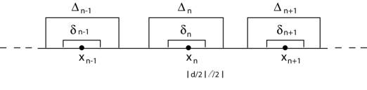
Figure 1: The picture shows the points $x_{n}$ associated to the different outcomes of an experiment, together with the intervals $\delta_{n}$ and $\Delta_{n}$ used for the proof of Theorem 1.

Up to now we have spoken only of the position of the pointer, but as we have said it is custom to refer the probabilities to the (numerical) outcomes of the measurement. To this end we introduce the following calibration function:

$$f(q_{t_{\makebox{\tiny F}}})\;=\;v_{n}\,\in\,{\mathcal{O}}\qquad\quad\text{iff:}\;\;q_{t_{\makebox{\tiny F}}}\,\in\,\Delta_{n},$$ (21)

which simply means that the outcome of the experiment is $v_{n}$ whenever the pointer, at the end of the measurement process, lies around the position $x_{n}$ of the graduate scale. In the above definition, we have chosen $\Delta_{n}$ as the relevant intervals in order to make the proof of the following theorem simpler: however, on a macroscopic scale the two sets of intervals ($\{\delta_{n}\}$ and $\{\Delta_{n}\}$) are practically identical. Note that, since we want different outcomes to correspond to different macroscopic configurations of the pointer, the intervals $\Delta_{n}$ should not overlap, which means that the distance between two consecutive points $x_{n}$ and $x_{n+1}$ along the graduate scale should be bigger that $d+\ell\simeq 10^{-6}$ m; this is of course a perfectly reasonable assumption.

We are now in the position to prove the following theorem, which is the cornerstone for the subsequent derivation of the Hilbert space formalism from the framework of DRMs.

Theorem 1. Let us consider an experiment globally described by the stave vector $|\psi_{t}\rangle$, let $q_{t}$ be the position of the (center of mass of the) pointer at time $t$ right before the measurement begins, and let $t_{\makebox{\tiny F}}$ be the time at which the experiment ends. Then:

$$\forall\,\,V\,\in\,{\mathcal{G}}:\qquad\left|{\mathbb{P}}_{f(q_{t_{\makebox{\tiny F}}})}[V]-{\mathbb{Q}}_{t_{\makebox{\tiny F}}}[V]\right|\;\leq\;2\left[\left(\frac{\sigma_{q}}{\ell}\right)^{2}+\eta\right],$$ (22)

where the probability measure ${\mathbb{Q}}_{t}$ is defined as follows:

$${\mathbb{Q}}_{t}[V]\;\equiv\;{\mathbb{E}}_{\mathbb{P}}[\langle\psi_{t}|P_{\Delta_{V}}|\psi_{t}\rangle],$$ (23)

and $P_{\Delta_{V}}$ is the projection operator on the (measurable) subset $\Delta_{V}\equiv f^{-1}(V)$, which is the subset of ${\mathbb{R}}$ of all positions of the pointer corresponding to a precise outcome $v$ among the possible outcomes belonging to $V$.

The above theorem is very powerful: according to the very general structures of DRMs, the probability distribution ${\mathbb{P}}_{f(q_{t_{\makebox{\tiny F}}})}$ of the outcomes of an experiment can, for all practical purposes, be replaced by the probability measure ${\mathbb{Q}}_{t_{\makebox{\tiny F}}}$ which has a the very simple mathematical expression given by Eq. (23). This is due to Eq. (22) and to the fact that, according to the typical numerical values for $\lambda,\eta$, $\sigma_{q}$ and $\ell$ given before, one has:

$$2\left[\left(\frac{\sigma_{q}}{\ell}\right)^{2}+\eta\right]\;\simeq\;2\times 10^{-16},$$ (24)

a vanishingly small value. We point out that Eq. (23) should not be confused with the quantum average value of the projection operator $P_{B}$ relative to the position of the pointer, as given by standard quantum mechanics. As a matter of fact, since an experiment always involves a macroscopic system, the one described by $|\psi_{t}\rangle$, a state vector which includes both the measured system and the measuring apparatus entails a dynamical evolution which is entirely different from that predicted by the Schrödinger equation, in particular it always keeps the measuring device in a state well localized in space. We now prove the theorem.

$$\left|{\mathbb{P}}_{f(q_{t_{\makebox{\tiny F}}})}[V]-{\mathbb{Q}}_{t_{\makebox{\tiny F}}}[V]\right| \equiv \left|{\mathbb{P}}[q_{t_{\makebox{\tiny F}}}^{-1}(\Delta_{V})]\;-\;{\mathbb{E}}_{\mathbb{P}}[\langle\psi_{t_{\makebox{\tiny F}}}|P_{\Delta_{V}}|\psi_{t_{\makebox{\tiny F}}}\rangle]\right|$$ (25)

$$= \left|\int_{q_{t_{\makebox{\tiny F}}}^{-1}(\Delta_{V})}d{\mathbb{P}}\;-\;\int_{\Omega}\langle\psi_{t_{\makebox{\tiny F}}}|P_{\Delta_{V}}|\psi_{t_{\makebox{\tiny F}}}\rangle\,d{\mathbb{P}}\right|$$

$$\leq \int_{q_{t_{\makebox{\tiny F}}}^{-1}(\Delta_{V})}(1-\langle\psi_{t_{\makebox{\tiny F}}}|P_{\Delta_{V}}|\psi_{t_{\makebox{\tiny F}}}\rangle)d{\mathbb{P}}\;+\;\int_{\Omega-q_{t_{\makebox{\tiny F}}}^{-1}(\Delta_{V})}\langle\psi_{t_{\makebox{\tiny F}}}|P_{\Delta_{V}}|\psi_{t_{\makebox{\tiny F}}}\rangle\,d{\mathbb{P}}$$

$$= \int_{q_{t_{\makebox{\tiny F}}}^{-1}(\Delta_{V})}\langle\psi_{t_{\makebox{\tiny F}}}|P_{{\mathbb{R}}-\Delta_{V}}|\psi_{t_{\makebox{\tiny F}}}\rangle d{\mathbb{P}}\;+\;\int_{q_{t_{\makebox{\tiny F}}}^{-1}({\mathbb{R}}-\Delta_{V})}\langle\psi_{t_{\makebox{\tiny F}}}|P_{\Delta_{V}}|\psi_{t_{\makebox{\tiny F}}}\rangle\,d{\mathbb{P}},$$

where $\Omega$ is the sample space on which the stochastic dynamics is defined. Let us define $\delta_{V}\equiv\cup_{n}\delta_{n}$ with $\delta_{n}\,\in\,\Delta_{V}$; the first of the two terms in the last line can be re-written as follows:

$$\int_{q_{t_{\makebox{\tiny F}}}^{-1}(\Delta_{V})}\langle\psi_{t_{\makebox{\tiny F}}}|P_{{\mathbb{R}}-\Delta_{V}}|\psi_{t_{\makebox{\tiny F}}}\rangle\,d{\mathbb{P}}\;=\;\int_{q_{t_{\makebox{\tiny F}}}^{-1}(\delta_{V})}\langle\psi_{t_{\makebox{\tiny F}}}|P_{{\mathbb{R}}-\Delta_{V}}|\psi_{t_{\makebox{\tiny F}}}\rangle\,d{\mathbb{P}}\;+\;\int_{q_{t_{\makebox{\tiny F}}}^{-1}(\Delta_{V}-\delta_{V})}\langle\psi_{t_{\makebox{\tiny F}}}|P_{{\mathbb{R}}-\Delta_{V}}|\psi_{t_{\makebox{\tiny F}}}\rangle\,d{\mathbb{P}};$$ (26)

according to the second property of DRMs listed above, the probability measure of the set $\Delta_{V}-\delta_{V}$ is smaller than $\eta$; thus, taking also into account that $\langle\psi_{t_{\makebox{\tiny F}}}|P_{{\mathbb{R}}-\Delta_{V}}|\psi_{t_{\makebox{\tiny F}}}\rangle\leq 1$, we can write:

$$\int_{q_{t_{\makebox{\tiny F}}}^{-1}(\Delta_{V}-\delta_{V})}\langle\psi_{t_{\makebox{\tiny F}}}|P_{{\mathbb{R}}-\Delta_{V}}|\psi_{t_{\makebox{\tiny F}}}\rangle\,d{\mathbb{P}}\;\leq\;\eta.$$ (27)

Regarding the first term on the right-hand-side of Eq. (26), we now show that the integrand $\langle\psi_{t_{\makebox{\tiny F}}}|P_{{\mathbb{R}}-\Delta_{V}}|\psi_{t_{\makebox{\tiny F}}}\rangle$ is extremely small for any $\omega\in\Omega$ such that $q_{t_{\makebox{\tiny F}}}$ lies within $\delta_{V}$. Defining $\psi(x)=\langle x|\psi_{t_{\makebox{\tiny F}}}\rangle$, we have of course

$$\langle\psi_{t_{\makebox{\tiny F}}}|P_{{\mathbb{R}}-\Delta_{V}}|\psi_{t_{\makebox{\tiny F}}}\rangle=\int d\{q\}\int_{{\mathbb{R}}-\Delta_{V}}dx\;|\psi_{t_{\makebox{\tiny F}}}(\{q\},x)|^{2},$$ (28)

where $\{q\}$ denote all degrees of freedom involved in the measurement, except the one for the center of mass of the pointer. Whenever $q_{t_{\makebox{\tiny F}}}$ belongs to $\delta_{V}$, we have that the parameter $\ell$ defining essentially the extension of the intervals $\Delta_{n}$, satisfies $\ell^{2}\leq(x-q_{t_{\makebox{\tiny F}}})^{2}$ for all $x\in{\mathbb{R}}-\Delta_{V}$; we get then the following inequality:

$$\ell^{2}\int d\{q\}\int_{{\mathbb{R}}-\Delta_{V}}dx\;|\psi_{t_{\makebox{\tiny F}}}(\{q\},x)|^{2} \leq \int d\{q\}\int_{{\mathbb{R}}-\Delta_{V}}dx\;(x-q_{t_{\makebox{\tiny F}}})^{2}|\psi_{t_{\makebox{\tiny F}}}(\{q\},x)|^{2}$$ (29)

$$\leq \int d\{q\}\int_{{\mathbb{R}}}dx\;(x-q_{t_{\makebox{\tiny F}}})^{2}|\psi_{t_{\makebox{\tiny F}}}(\{q\},x)|^{2}\;\equiv\;\sigma_{q}^{2}.$$

Eqs. (26), (27) and (29) lead to the following result:

$$\int_{q_{t_{\makebox{\tiny F}}}^{-1}(\Delta_{V})}\langle\psi_{t_{\makebox{\tiny F}}}|P_{{\mathbb{R}}-\Delta_{V}}|\psi_{t_{\makebox{\tiny F}}}\rangle d{\mathbb{P}}\;\leq\;\left(\frac{\sigma_{q}}{\ell}\right)^{2}+\eta$$ (30)

A completely symmetric argument holds for the second and last terms at the right-hand-side of equation (25) as well, hence the theorem is proven.

To summarize, we have shown that in measurement-like situations it is fully legitimate, as a consequence of the reducing dynamics of DRM, to use the probability measure ${\mathbb{Q}}_{t}$ in place of ${\mathbb{P}}_{f(q_{t})}$ to compute the probabilities of the possible outcomes of an experiment.

III.2.2 The emergence of the Hilbert-space operator formalism

Let us now focus our attention on the probability measure ${\mathbb{Q}}_{t}$ which, according to the definition (23), can be re-written also as:

$${\mathbb{Q}}_{t}[V]\;\equiv\;\makebox{Tr}\,[\rho_{t}\,({\mathbb{I}}_{\{q\}}\otimes P_{\Delta_{V}})]\qquad\quad V\,\in\,{\mathcal{G}},$$ (31)

where ${\mathbb{I}}_{\{q\}}$ is the identity operator acting on the space of all degrees of freedom of the experiment, except the one referring to the center of mass of the pointer. The above expression is a consequence of the well-known formula typical of DRMs rev1 :

$${\mathbb{E}}_{\mathbb{P}}[\langle\psi_{t}|O|\psi_{t}\rangle]\;=\;\makebox{Tr}\,[O\rho_{t}]\qquad\quad\text{with: $\rho_{t}\equiv{\mathbb{E}}_{\mathbb{P}}[|\psi_{t}\rangle\langle\psi_{t}|]$},$$ (32)

where $O$ is any suitable operator. We remind the reader that the state vector $|\psi_{t}\rangle$ (thus also $\rho_{t}$) refers both to the (whole) state of the measuring device as well as to the state of the microscopic system. Regarding the initial state $|\psi_{t_{0}}\rangle$ (or, equivalently, $\rho_{t_{0}}$), right before the experiment begins, we make the following assumption:

Assumption 1.

At the beginning of the experiment ($t=t_{0}$), the state of the micro-system and that of the apparatus are factorized:

$$\qquad\rho_{t_{0}}\;=\;\rho^{S}_{t_{0}}\otimes\rho^{A}_{t_{0}},$$ (33)

where $\rho^{S}_{t_{0}}=|\psi^{S}_{t_{0}}\rangle\langle\psi^{S}_{t_{0}}|$ represents the initial state of the microscopic system, which we assume to be pure, while $\rho^{A}_{t_{0}}$ represents the initial state of the apparatus.

This initial factorization of the two states is a very natural assumption to make, since otherwise the microscopic system would not be in any defined state, whose property the experiment should detect. Moreover, we recall the following important property characterizing dynamical reduction models:

Property 3.

The dynamical evolution $\Sigma_{(t_{0},t_{\makebox{\tiny F}})}$ mapping the density matrix $\rho_{t_{0}}$ describing the global state prior to the experiment, into the final state $\rho_{t_{\makebox{\tiny F}}}$ after the experiment, is of the quantum dynamical semigroup type, thus, in particular, linear and trace-preserving.

According to the above two assumptions, we can write ${\mathbb{Q}}_{t}$, computed at time $t=t_{\makebox{\tiny F}}$, as follows:

$${\mathbb{Q}}_{t_{\makebox{\tiny F}}}[V]\;\equiv\;\makebox{Tr}\,[\Sigma_{(t_{0},t_{\makebox{\tiny F}})}(\rho^{S}_{t_{0}}\otimes\rho^{A}_{t_{0}}){\mathbb{I}}_{\{q\}}\otimes P_{\Delta_{V}}]\qquad\quad V\,\in\,{\mathcal{G}},$$ (34)

for any fixed $V\in{\mathcal{G}}$. Assuming now that $|\psi^{S}_{t_{0}}\rangle$ can run over the entire Hilbert space ${\mathcal{H}}^{S}$, the above expression defines the diagonal part of the following bounded sesquilinear form:

$$\begin{array}[]{ccl}{\mathcal{H}}^{S}\otimes{\mathcal{H}}^{S}&\longrightarrow&{\mathbb{C}}\\ (|\psi^{S}_{t_{0}}\rangle,|\phi^{S}_{t_{0}}\rangle)&\longrightarrow&\makebox{Tr}\,[\Sigma_{(t_{0},t_{\makebox{\tiny F}})}(|\psi^{S}_{t_{0}}\rangle\langle\phi^{S}_{t_{0}}|\otimes\rho^{A}_{t_{0}}){\mathbb{I}}_{S}\otimes P_{\Delta_{V}}];\end{array}$$ (35)

which, according to the Riesz representation theorem, can be written as follows:

$${\mathbb{Q}}_{t_{\makebox{\tiny F}}}[V]\quad=\quad\langle\psi^{S}_{t_{0}}|O_{V}|\psi^{S}_{t_{0}}\rangle\quad=\quad\text{Tr}\,[\rho_{t_{0}}O_{V}],$$ (36)

where $O_{V}$ is a bounded linear operator in ${\mathcal{H}^{S}}$. In our case, $O_{V}$ turns out to be also self-adjoint and defines a POVM from the measurable space of the possible outcomes $({\mathcal{O}},{\mathcal{G}})$ to the Hilbert space ${\mathcal{H}}^{S}$ of the micro-system. This is the desired result, which we formalize in the following theorem:

Theorem 2. According to the properties of DRMs stated before (properties 1–3), according to assumption 1 and, within the limits set by Theorem 1, one can write:

$${\mathbb{P}}_{f(q_{t_{\makebox{\tiny F}}})}[V]\quad\simeq\quad\langle\psi^{S}_{t_{0}}|O_{V}|\psi^{S}_{t_{0}}\rangle\qquad\quad\forall\,\,V\,\in\,{\mathcal{G}}.$$ (37)

In other words, the probability that the outcome of a given experiment belongs to the measurable subset $V$ of the set ${\mathcal{O}}$ of possible outcomes can be (with very high accuracy) expressed as the average value of the effect $O_{V},V\in{\mathcal{G}}$, of a POVM, over the initial state $|\psi^{S}_{t_{0}}\rangle$ of the microscopic system.

We have thus recovered the operator formalism of standard quantum mechanics.

It is interesting to compare Eq. (36) with Eq. (34):

$${\mathbb{Q}}_{t_{\makebox{\tiny F}}}[V]\quad=\quad\makebox{Tr}\,[\Sigma_{(t_{0},t_{\makebox{\tiny F}})}(\rho^{S}_{t_{0}}\otimes\rho^{A}_{t_{0}}){\mathbb{I}}_{S}\otimes P_{\Delta_{V}}]\quad=\quad\text{Tr}\,[\rho_{t_{0}}O_{V}];$$ (38)

the middle term of the above equation provides the true physical description of the experiment: it gives the probability for the pointer to lie within a well-defined region along the graduate scale at time $t_{\makebox{\tiny F}}$; on the other hand, the last term provides the compact (and very handy) quantum way of expressing such probabilities in terms of the initial state of the micro-system. A couple of further comments are at order.

1. Clearly, since a wave function has always a spatial extension, the width of the intervals $\Delta_{n}$ can not be set equal to zero. This means that, according to DRMs, only experiments having at most a countable number of outcomes can be performed. This of course includes all physically realizable experiments, while those having a continuous number of outcomes represent a mathematical idealization.

2. Nowhere in our analysis we have explicitly used the fact that the probabilities of the possible outcomes of the experiment, as predicted by DRMs, practically coincides with quantum probabilities. However, such a feature of DRMs is implicitly contained in property 3, i.e. in the fact that the evolution law for the statistical operator is linear; the reason is the following. When a jump process of the form (1) occurs on the $n$-th particle of a many-particle system, a density matrix $\rho\equiv\sum_{i}c_{i}|\psi_{i}\rangle\langle\psi_{i}|$ changes, in accordance to axiom B, as follows:

$$\rho\equiv\sum_{i}c_{i}|\psi_{i}\rangle\langle\psi_{i}|\quad\longrightarrow\quad\sum_{i}c_{i}\int d^{3}{\bf x}\;p({\bf x})\;\frac{L_{n}({\bf x})|\psi_{i}\rangle\langle\psi_{i}|L_{n}({\bf x})}{\|L_{n}({\bf x})\psi_{i}\rangle\|^{2}},$$ (39)

where $p({\bf x})$ is the probability density for a jump to occur in ${\bf x}$. As we see, the above evolution is not linear in $\rho$, unless we require $p({\bf x})$ to be of the form (2), which agrees with the Born probability rule.

IV Reproducibility and PVM

The example we have discussed in Sec. II belongs to a particular subclass of experiments, because it can be associated to a PVM, while the general theorem of the previous section shows that experiments are in general associated to POVM, which are more general than PVM. In this section we show that the possibility of associating a PVM to an experiment is strictly connected to the reproducibility of the experiment itself: since on standard books on quantum mechanics it is (implicitly) assumed that experiments are reproducible, the analysis shows why usually experiments are associated to projection operators.

We say that an experiment is reproducible if it can be performed many times on the same physical system and, each time we perform two runs in a row, one right after the other, the second one always yields the same outcome as the first one. In order to give a more rigorous definition, we first have to recall another important feature of DRMs:

Property 4.

At the end of a measurement process, the final state $|\psi_{t_{\makebox{\tiny F}}}\rangle$ of the whole system is, to a great accuracy, a factorized state of the system and the apparatus: $|\psi_{t_{\makebox{\tiny F}}}\rangle\simeq|\psi_{t_{\makebox{\tiny F}}}^{S}\rangle\otimes|\psi_{t_{\makebox{\tiny F}}}^{A}\rangle$. Accordingly, the vector $|\psi^{S}_{t_{0}}\rangle$ representing the state of the microscopic system right before the experiment began, changes to a new (normalized) state $|\psi^{S}_{t_{\makebox{\tiny F}}}\rangle$, which depends in general both on $|\psi^{S}_{t_{0}}\rangle$ and on the stochastic dynamics of the interaction between the system $S$ and the apparatus $A$.

In the following, when convenient we will write $|\psi^{S}_{t_{\makebox{\tiny F}}}/\psi^{S}_{t_{0}}\rangle$ in place of $|\psi^{S}_{t_{\makebox{\tiny F}}}\rangle$, to stress the dependence of the final state on the initial one; moreover, we will often write $|\psi^{S,v_{n}}_{t_{\makebox{\tiny F}}}\rangle$ in place of $|\psi^{S}_{t_{\makebox{\tiny F}}}\rangle$ to signify that $|\psi^{S}_{t_{\makebox{\tiny F}}}\rangle$ is the state to which the systems $S$ is reduced at the end of the first experiment in which we suppose that the outcome $v_{n}$ has been obtained. Let $|\psi^{2:v_{n}}_{t}\rangle$ describe the time evolution during the second experiment, when the initial state at time $t_{0}^{\prime}$ at which the second experiment takes place is assumed to be: $|\psi^{2:v_{n}}_{t_{0}^{\prime}}\rangle=|\psi^{S,v_{n}}_{t_{\makebox{\tiny F}}}\rangle\otimes|\psi^{A}_{t_{0}^{\prime}}\rangle$. A reproducible experiment is defined as follows.

Definition 3: Reproducible experiment. An experiment on a physical system $S$ is said to be reproducible if and only if:

1. The experiment can be performed on $S$ at least twice; moreover, the Hilbert space ${\mathcal{H}}$ of vectors describing the possible states of $S$ before the measurement is the same as the Hilbert space of vectors describing the possible states of the system after the measurement; in other words, the totality of the possible final states $|\psi^{S}_{t_{\makebox{\tiny F}}}\rangle$ must span ${\mathcal{H}}$:

   $$\operatorname{span}\set{}{\psi^{S}_{t_{\makebox{\tiny F}}}/\psi^{S}_{t_{0}}\rangle,\;\;|\psi^{S}_{t_{0}}\rangle\,\in\,{\mathcal{H}}}=\mathcal{H}.$$ (40)

2. Let us suppose that two experiments are done, one immediately after the other; let ${\mathbb{P}}^{v_{n}}_{f(q_{t_{\makebox{\tiny F}}^{\prime}})}$ be the probability distribution of the outcomes of the second experiment, assuming that $|\psi^{S:v_{n}}_{t_{\makebox{\tiny F}}}\rangle$ has been taken as the initial state of the microscopic system for the second experiment, i.e. assuming that the outcome of the first experiment is $v_{n}$. We then require that:

   $${\mathbb{P}}^{v_{n}}_{f(q_{t_{\makebox{\tiny F}}^{\prime}})}[V]=1,\qquad\forall\,\,V\,:v_{n}\in V$$ (41)

   i.e. that the outcome of the second run of the experiment belongs to $V$ with certainty.

Let us briefly comment on the above definition. The first request in the definition above excludes experiments which alter the nature of the physical system, e.g. because they destroy it, or one of its parts, or because they transform it in a new physical system with a space of states $\mathcal{H}^{\prime}$ different from the original space $\mathcal{H}$. The second request just embodies the idea of reproducibility, by assuring that the same outcome is obtained with certainty when the experiment is performed twice. Now we can state the following theorem:

Theorem 3: Reproducible experiment. Let us consider an experiment which, according to Theorem 2, is associated to a POVM $\{O_{V}\}_{V}$. If the experiment is reproducible, and within the limits of replacing the probability ${\mathbb{P}}^{v_{n}}_{f(q_{t_{\makebox{\tiny F}}^{\prime}})}$ with the probability ${\mathbb{Q}}^{v_{n}}_{t_{\makebox{\tiny F}}^{\prime}}[V]={\mathbb{E}}_{\mathbb{P}}[\langle\psi^{2:v_{n}}_{t_{\makebox{\tiny F}}^{\prime}}|P_{\Delta_{V}}|\psi^{2:v_{n}}_{t_{\makebox{\tiny F}}^{\prime}}\rangle]$, then the POVM is a PVM.

The proof of the theorem is given in Ref. bm ; here we propose a simplified version of it. We first of all notice that, given a self-adjoint positive semidefinite operator $O$ with bounds $0\leq O\leq I$, then

$$\langle\psi|O|\psi\rangle=1 \qquad\Rightarrow\qquad O|\psi\rangle=|\psi\rangle$$ (42)

$$\langle\psi|O|\psi\rangle=0 \Rightarrow O|\psi\rangle=|\omega\rangle,$$ (43)

where $|\omega\rangle$ is the null vector. To show this, let us write ${\mathcal{H}}=\mathcal{H}_{1}\oplus\mathcal{H}_{1}^{\perp}$, where $\mathcal{H}_{1}$ is the subspace of all eigenstates of $O$ corresponding to the eingenvalue 1 and $\mathcal{H}_{1}^{\perp}$ its orthogonal complement. Let $|\psi\rangle$ be a normalized vector, which we decompose in: $\ket{\psi}=\ket{\psi_{\parallel}}+\ket{\psi_{\perp}}$, where $\ket{\psi_{\parallel}}\in\mathcal{H}_{1}$ and $\ket{\psi_{\perp}}\in\mathcal{H}_{1}^{\perp}$. It follows that:

$$\langle\psi|O|\psi\rangle=1\qquad\Rightarrow\qquad\Braket{\psi_{\perp}}{O}{\psi_{\perp}}=\Braket{\psi_{\perp}}{\psi_{\perp}}.$$ (44)

On the other hand, the property $0\leq O\leq I$ implies that $O$ acts on the subspace $\mathcal{H}_{1}^{\perp}$ like a contraction, i.e. that $\|O\ket{\psi_{\perp}}\|<\|\ket{\psi_{\perp}}\|$, unless $\ket{\psi_{\perp}}=|\omega\rangle$. This contraction property, together with the Cauchy-Schwarz inequality, gives

$$\braket{\psi_{\perp}}{O}{\psi_{\perp}}\;<\;\braket{\psi_{\perp}}{\psi_{\perp}}\qquad\text{unless}\;\;\ket{\psi_{\perp}}=|\omega\rangle.$$ (45)

Now, Eqs. (44) and (45) are incompatible unless $\ket{\psi_{\perp}}=|\omega\rangle$, which proves Eq. (42). In a similar way one can prove also Eq. (43).

Coming back to the probability measure ${\mathbb{Q}}^{v_{n}}_{t_{\makebox{\tiny F}}^{\prime}}$, according to the analysis of the previous section and to the hypotheses of our theorem, we can write, for any $V\subseteq{\mathcal{G}}$:

$${\mathbb{Q}}^{v_{n}}_{t_{\makebox{\tiny F}}^{\prime}}[V]\;=\;\langle\psi^{S:v_{n}}_{t_{\makebox{\tiny F}}}|O_{V}|\psi^{S:v_{n}}_{t_{\makebox{\tiny F}}}\rangle\;=\;\left\{\begin{array}[]{ll}1&\text{if}\;v_{n}\in V,\\ 0&\text{else.}\end{array}\right.$$ (46)

Let ${\mathcal{H}}_{1}^{V}$ be the subspace of all eigenstates of $O_{V}$ corresponding to the eingenvalue 1, and ${\mathcal{H}}_{0}^{V}$ be the subspace of all eigenstates corresponding to the eingenvalue 0; according to (46), and to the fact that $\text{span}\{|\psi^{S:v_{n}}_{t_{\makebox{\tiny F}}}\rangle\}\equiv{\mathcal{H}}$, we can write: ${\mathcal{H}}={\mathcal{H}}_{1}^{V}\oplus{\mathcal{H}}_{0}^{V}$. This result proves that $O_{V}$ is an orthogonal projector on $\mathcal{H}$, with support in ${\mathcal{H}}_{1}^{V}$. Hence the POVM $\set{O_{V}}_{V}$ is a PVM.

The ideal measurements usually considered in many QM textbook, i.e., those obeying the rule of the Wave-Packet Reduction (WPR) postulate, are reproducible, and therefore the POVM associated to them reduces to a PVM. When this happens, the experiment can be entirely characterized, with respect to its statistical properties, by a single self-adjoint operator, as is usually done in quantum mechanics.

V The “tail problem”; the Stern-Gerlach experiment revisited

One of the reason why, with reference to theorem 1, the two probabilities ${\mathbb{P}}_{q_{t_{\makebox{\tiny F}}}}$ and ${\mathbb{Q}}_{t_{\makebox{\tiny F}}}$ are not strictly equal is that, even when $q_{t}\in\delta_{n}$, the wave function for the center of mass of the pointer has not a compact support contained in the interval $\Delta_{n}$, but it has tails spreading out to infinity; such tails, being extremely small (in the sense that the integral of the square modulus of the wave function over the region laying outside $\Delta_{n}$, assuming that its center is contained within $\delta_{n}$, is very small), give not rise to any problem in connection with the interpretation of the theory and its physical predictions.

In this section we want to point out that precisely the same problem with tails occur also in standard quantum mechanics. Let us take as an example the Stern-Gerlach experiment: this is often used in textbooks as the paradigmatic experiment which illustrates the correspondence between observables and self-adjoint operators. What textbooks usually provide is just a simplified description of the truly observed experimental results; a more realistic analysis which takes into account also the spatial (beside spin) degrees of freedom of the atoms sent through the apparatus would show that tails emerge also here, which (just in principle) give rise to some potential problems in interpreting the outcome of the experiment, and in associating a self-adjoint operator to it. In this section we perform such a kind of analysis, we discuss the role of the tails of the wave function of the atoms and we make precise the sense in which it is legitimate to associate the usual spin operator $S_{z}$ to the experiment.

As it is well known, Stern and Gerlach used an oven to produce and send a beam of silver atoms through an inhomogeneous magnetic field, letting it eventually impinge on a glass plate. In order to analyze the effect of the magnetic field on the beam, two separate experiments were originally sg performed: one with the magnet generating the field turned on, with a run time of 8 hours, another with the magnet turned off, with a run time of 4.5 hours. In the magnet-off case, a single bar of silver approximately 1.1 mm long and 0.06–0.1 mm wide was deposited on the glass plate. In the magnet-on case, a pair-of-lips shape appeared on the glass: the shape was 1.1 mm long, one lip was 0.11 mm wide, the other was 0.20 mm wide; both lips appeared deflected with respect to the position of the magnet-off bar, and the maximum gap between the upper and lower lips was approximately of the order of magnitude of the width of the lips. Stern and Gerlach made only visual observations through a microscope, with no statistics on the distributions: they did not obtain “two spots” as it is usually stated on textbooks, and though the beam was clearly split in two distinguishable parts, these were not disjoint. They accounted for the experiment as exhibiting the property of “space quantization in a magnetic field.”

Let us give a simplified mathematical description of the experiment, taking however into account not only the spin, but also the spatial degrees of freedom of (the center of mass of) the silver atoms boo . The silver atoms of a Stern-Gerlach experiment can be treated as spin one-half elementary particles to a very high degree of accuracy; let us assume that they are initially prepared in an (arbitrary) spin state

$$\ket{c_{+},c_{-}}=c_{+}\ket{+}+c_{-}\ket{-},\qquad\text{($|c_{+}|^{2}+|c_{-}|^{2}=1$)},$$ (47)

where $\ket{+}$ and $\ket{-}$ denote the usual normalized eigenstates of $S_{z}$. The wave function describing the center of mass of the atom at the initial time $t=0$ can be taken to be a normalized Gaussian wave packet

$$G({\bf x};{\bf x}_{0},{\bf p}_{0},\Delta_{\bf x})=\braket{{\bf x}}{{\bf x}_{0},{\bf p}_{0},\Delta_{\bf x}}$$ (48)

centered around the position ${\bf x}_{0}$, traveling along the $x$-axis towards the region where the magnet is located, with mean value of momentum ${\bf p}_{0}$ and spatial spread $\Delta_{\bf x}$, extremely well localized with respect to the dimensions of the region where the magnetic field is different from 0.

Let us model the interaction between the atom and the magnetic field, which we treat as a static external field, by the usual Hamiltonian operator $H_{\mathrm{SG}}=\bm{\mu}\cdot{\bf B}$ with $\bm{\mu}=k\bm{\sigma}$, ${\bf B}$ the magnetic field, $\bm{\sigma}=(\sigma_{x},\sigma_{y},\sigma_{z})$ the three Pauli operators, and $k$ a known constant whose value is irrelevant for the following discussion. Denoting by $\hat{\bf z}$ the unit vector along the $z$-axis, let us assume that the inhomogeneous magnetic field is ${\bf B}=(B_{0}-bz)\,\hat{\bf z}$ inside the spatial region where the magnet is located and with a negligible gradient outside it. Finally, to simplify the matter as far as possible, let us adopt the “impulsive measurement” assumption, which amounts to ignoring the free evolution of the silver atom while it is interacting with the magnetic field, and let us suppose that the time interval $\tau$ between the emission of the silver atom from the oven and the moment when it impinges on the glass plate is so small that the spread $\Delta_{\bf x}$ of its wave packet does not vary appreciably.

With these premises, a simple calculation shows that the state of the silver atom at the time $t=\tau$, after it went through the inhomogeneous magnetic field region and just before the detection by the glass plate, is

$$\ket{\psi_{\tau}} =c_{+}\ket{{\bf x}_{+},{\bf p}_{+},\Delta_{\bf x}}\otimes\ket{+}+c_{-}\ket{{\bf x}_{-},{\bf p}_{-},\Delta_{\bf x}}\otimes\ket{-},$$ (49)

where the wave functions $G({\bf x};{\bf x}_{\pm},{\bf p}_{\pm},\Delta_{\bf x})=\braket{{\bf x}}{{\bf x}_{\pm},{\bf p}_{\pm},\Delta_{\bf x}}$ are normalized Gaussian packets of mean momentum ${\bf p}_{\pm}$ and mean position ${\bf x}_{\pm}$ given by:

$${\bf p}_{\pm}\;=\;{\bf p}_{0}\pm kb\tau\,\hat{\bf z},\qquad\quad{\bf x}_{\pm}\;\simeq\;{\bf x}_{0}+\frac{{\bf p}_{0}}{m}\,\tau\pm\frac{kb}{m}\,\tau^{2}\,\hat{\bf z}.$$ (50)

The detection process by means of the glass plate can be modeled by associating to the plate the operator $Z\equiv Z_{+}-Z_{-}$, acting on the spatial degrees of freedom, where $Z_{+}$ and $Z_{-}$ are the two projection operators corresponding to the localization in the upper ($z\geq 0$) or lower ($z\leq 0$) half parts of the plate. Recalling that we choose a normalized vector to represent the initial state, the corresponding probabilities according to standard quantum mechanical rules are then easily seen to be

$${\mathbb{P}}_{(c_{+},c_{-})}(\pm 1) = \braket{\psi_{\tau}}{Z_{\pm}\otimes I_{{\mathbb{C}}^{2}}}{\psi_{\tau}}$$ (51)

$$= |c_{+}|^{2}\braket{{\bf x}_{+},{\bf p}_{+},\Delta_{\bf x}}{Z_{\pm}}{{\bf x}_{+},{\bf p}_{+},\Delta_{\bf x}}\;+\;|c_{-}|^{2}\braket{{\bf x}_{-},{\bf p}_{-},\Delta_{\bf x}}{Z_{\pm}}{{\bf x}_{-},{\bf p}_{-},\Delta_{\bf x}}$$

By looking at equation (51), we immediately see that the probability to observe an outcome in, say, the upper part of the screen, is not $|c_{+}|^{2}$, as one can find in the textbook descriptions of the experiment, because the two wave functions $G({\bf x};{\bf x}_{\pm},{\bf p}_{\pm},\Delta_{\bf x})$ are not localized sharply in (respectively) the upper and lower parts of the glass plate. Indeed, the tail of the “+” wave function $G({\bf x};{\bf x}_{+},{\bf p}_{+},\Delta_{\bf x})$ which lies in the lower part does not contribute at all to ${\mathbb{P}}_{(c_{+},c_{-})}(+1)$, while the tail of the “$-$” wave function $G({\bf x};{\bf x}_{-},{\bf p}_{-},\Delta_{\bf x})$ laying in the upper part does contribute (see Fig. 2). Needless to say, this is not a disfeature due to the use of a Gaussian wave-packet: the whole analysis could be repeated practically unaltered for an arbitrary initial wave packet, because even if one starts with a wave packet with compact support, the free evolution would immediately and unavoidably spread it all over space.

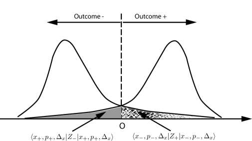
Figure 2: Typical (schematic) spatial distribution of the superposition of two Gaussian wave functions in a Stern-Gerlach experiment. The wave function corresponding to the outcome “+” has a tail spreading in the region corresponding to the outcome “$-$”, and vice-versa.

However, provided the initial wave packet is sufficiently well localized both in position as well as in momentum (within the limits allowed by the Heisenberg principle, of course), and the spatial separation of the two final wave packets is much greater than their spatial spreads, i.e. $2kb\tau^{2}/m\gg\Delta_{\bf x}$ the “crossed” contributions of the tails, namely $\braket{{\bf x}_{+},{\bf p}_{+},\Delta_{\bf x}}{Z_{-}}{{\bf x}_{+},{\bf p}_{+},\Delta_{\bf x}}$ and $\braket{{\bf x}_{-},{\bf p}_{-},\Delta_{\bf x}}{Z_{+}}{{\bf x}_{-},{\bf p}_{-},\Delta_{\bf x}}$, are small compared with the uncrossed contributions, and the textbook approximation ${\mathbb{P}}_{(c_{+},c_{-})}(\pm 1)=|c_{\pm}|^{2}$ can be meaningfully recovered.

It is interesting to restate the previous argument in the following way, by observing that equation (51) can be rewritten in terms of the initial spin state $\ket{c_{+},c_{-}}$ as

$${\mathbb{P}}_{(c_{+},c_{-})}(\pm 1)=\Braket{c_{+},c_{-}}{O_{\pm}}{c_{+},c_{-}}$$ (52)

where the two effects $O_{\pm}$ are:

$$O_{\pm}\;\equiv\;\braket{{\bf x}_{+},{\bf p}_{+},\Delta_{\bf x}}{Z_{\pm}}{{\bf x}_{+},{\bf p}_{+},\Delta_{\bf x}}|+\rangle\langle+|\;+\;\braket{{\bf x}_{-},{\bf p}_{-},\Delta_{\bf x}}{Z_{\pm}}{{\bf x}_{-},{\bf p}_{-},\Delta_{\bf x}}|-\rangle\langle-|$$ (53)

acting on the spin Hilbert space ${\mathbb{C}}^{2}$. We thus obtain a result we are now used to: the probability distribution of the outcomes has been expressed as the average value of the effects of a POVM over the initial state of the microscopic quantum system. However, since the wave packets are spread out in space, we see that the effects (53) are not projection operators, i.e., $O_{\pm}^{2}\neq O_{\pm}$. Concluding, the observable associated to the Stern-Gerlach experiment is not exactly represented by the operator $S_{z}$ (or, equivalently, by the PVM given by $|+\rangle\langle+|$ and $|-\rangle\langle-|$): it is rather a generalized observable described by the POVM formed by the two effects $O_{\pm}$. Thus, to be rigorous, also within standard Quantum Mechanics the association of the operator $S_{z}$ to a Stern-Gerlach experiment is just an approximation, whose range of validity has been made clear by the previous discussion: indeed, when the crossed contributions of the tails of the two Gaussian wave functions are negligible with respect to the uncrossed ones, we have

$$O_{+}\;\simeq\;|+\rangle\langle+|\qquad\text{and}\qquad O_{-}\;\simeq\;|-\rangle\langle-|,$$ (54)

so that the POVM $\{O_{+},O_{-}\}$ associated to the experiment approximately becomes the spectral PVM $\{|+\rangle\langle+|,|-\rangle\langle-|\}$ of the spin operator $S_{z}$.

VI Observables as self-adjoint operators in classical mechanics: an example from classical electromagnetic theory.

From the previous analysis one should have grasped that the operator formalism for describing the outcome of experiments is not a peculiar feature of Quantum Mechanics but, according to the Riesz representation theorem, it can be applied whenever the states of physical systems are represented by vectors of a linear vector space and the outcome of an experiment depends “quadratically” on the initial state of the system being measured. As such, there is no reason why it should not be possible to apply such a formalism also to classical systems: to illustrate this fact, we now give an example taken from classical electromagnetic theory.

Let us confine our attention to a monochromatic plane wave of frequency $\omega$ traveling in the vacuum in some given direction $\hat{\bf n}$ (i.e., with wave vector ${\bf k}=\omega\hat{\bf n}$). Such a wave is completely characterized by the electric field

$${\bf E}(t,{\bf x})=\text{Re}\,(\bm{\epsilon}\exp\left[\mathrm{i}\left(\omega t-{\bf k}\cdot{\bf x}\right)\right]);$$ (55)

the complex wave amplitude $\bm{\epsilon}$ expresses both the intensity as well as the polarization state of the wave. Accordingly, taking into account the linearity of Maxwell’s equations and the fact that the wave intensity $I$ can be written in terms of $\bm{\epsilon}$ by means of the canonical complex scalar product,

$$I=\bm{\epsilon}^{*}\cdot\bm{\epsilon},$$ (56)

we see that, if we limit our attention to the degrees of freedom contained in the wave amplitude alone, ignoring the spatial ones, a monochromatic plane wave qualifies as a physical system whose states belong to the Hilbert space ${\mathbb{C}}^{2}$ and on which experiments (typically detection of the intesity) represented by quadratic forms can be performed.

One of the simplest examples of such a kind of experiment on a monochromatic plane wave can be constructed by letting the wave impinge on a linear Polaroid and by measuring the transmitted intensity. To further simplify the matter, let us restrict to the case of a linearly polarized monochromatic plane wave, i.e., let us assume $\bm{\epsilon}\in{\mathbb{R}}^{2}$. Experience shows that in such a situation the transmitted wave intensity $I_{f}$ depends on the angle between the directions of polarization of the wave and the filter according to the Malus law:

$$I_{f}\;=\;I_{i}\cos^{2}\theta,$$ (57)

where $I_{i}=\bm{\epsilon}\cdot\bm{\epsilon}$ is of course the incident wave intensity and, if $\hat{\bm{\eta}}$ is the polarization direction of the filter, $\cos\theta=\bm{\epsilon}\cdot\hat{\bm{\eta}}/\|\bm{\epsilon}\|$. Accordingly, Malus law (57) can be re-written as,

$$I_{f}\;=\;(\hat{\bm{\eta}}\cdot\bm{\epsilon})^{2},$$ (58)

and we easily recognize that the outcome of the experiment (the output intensity $I_{f}$) is a quadratic form of the initial state of the wave (its polarization $\bm{\epsilon}$). Then, according to the Riesz representation theorem, we can express $I_{f}$ in terms of a bounded linear operator $O$ as follows (we now pass to the Dirac notation to highlight the conclusion):

$$I_{f}(\hat{\bm{\eta}})\;=\;\braket{\bm{\epsilon}}{O_{\hat{\bm{\eta}}}}{\bm{\epsilon}}\qquad\quad O_{\hat{\bm{\eta}}}\;=\;|\hat{\bm{\eta}}\rangle\langle\hat{\bm{\eta}}|.$$ (59)

Of course, in the present example, the average value of the operator $O_{\hat{\bm{\eta}}}$ over the initial state of the micro-system does not represent the average of the possible outcomes weighted with their probabilities, but it is simply the (deterministic) value of the output intensity.

Let us note that this example also shows that non-commutativity, which is usually considered as a characteristic trait of quantum mechanics, can and does arise in classical and deterministic contexts as well. Indeed, by taking into account the fact that the transmitted wave is polarized along the direction of the filter:

$$\ket{\bm{\epsilon}_{\text{out}}}\;=\;\ket{\hat{\bm{\eta}}}\braket{\hat{\bm{\eta}}}{\bm{\epsilon}_{\text{in}}},$$ (60)

and by considering two successive arbitrarily oriented filters, we see that the transmitted intensity

$$I_{f}=I_{i}\cos^{2}\theta_{1}\cos^{2}(\theta_{2}-\theta_{1})$$ (61)

of the wave after the two filters depends in general on their respective order. The mathematical counterpart of this property is that the two operator $O_{\hat{\bm{\eta}}_{1}}$ and $O_{\hat{\bm{\eta}}_{2}}$ associated to the two experiments do not commute, a part from the very special orientations which correspond to $\ket{\hat{\bm{\eta}}_{1}}=\pm\ket{\hat{\bm{\eta}}_{2}}$ or $\braket{\hat{\bm{\eta}}_{1}}{\hat{\bm{\eta}}_{2}}=0$.

VII Conclusions

In this paper we have shown how the Hilbert-space operator formalism—i.e., the use of self-adjoint operators and, more generally, of POVM to describe experiments on quantum systems—can be recovered within the context of DRMs: it can be derived from the dynamical laws of DRMs satisfying the very general assumptions that we have analyzed in section III.2 as a compact way to express the statistical properties of the outcomes of measurement-like experiments. It is worthwhile stressing once again that within the context of DRMs the operator formalism has no special ontological meaning: as this paper shows in detail, it is merely a convenient tool that can be used to describe certain experiments that we are accustomed to think of as “measurements.”

This and the previous analysis prove that DRMs represent a well-grounded theory, whose ontology is clearly specified and consistent with our macroscopic perceptions, deprived from the typical paradoxes of quantum mechanics which are connected to the special roles that the theory attributes to “measurement processes” and “observables”.

We consider the results of this paper as an important step which completes, at the non-relativistic level, the general line of though and the world view which has inspired the dynamical reduction program, both at the formal and interpretational level.

- (1) G.C. Ghirardi, A. Rimini and T. Weber, Phys. Rev. D 34, 470 (1986).
- (2) A. Bassi and G.C. Ghirardi, Phys. Rept. 379, 257 (2003).
- (3) P. Pearle, in: “Open Systems and Measurement in Relativistic Quantum Theory”, Lecture Notes in Physics 526 (1999).
- (4) P. Pearle, Phys. Rev. A 39, 2277 (1989).
- (5) G.C. Ghirardi, A. Rimini and T. Weber. Phys. Rev. A 42, 78 (1990).
- (6) S.L. Adler, Quantum Theory as an emergent phenomenon (Chapter 6), Cambridge University Press, Cambridge (2004).
- (7) G.C. Ghirardi, R. Grassi and F. Benatti, Found. Phys. 25, 5 (1995).
- (8) J.S. Bell, Speakable and Unspeakable in Quantum Mechanics, 2nd edition (Cambridge University Press, Cambridge 2004), p. 166.
- (9) D. Dürr, S. Goldstein and N. Zanghì, Journ. Stat. Phys. 116, 959 (2004).
- (10) A. Bassi and D.G.M. Salvetti, Journ. Phys. A: Math. Theor. 40, 9859 (2007).
- (11) W. Gerlach and O. Stern, Zeits. Phys. 9, 349 (1922).
- (12) P. Busch, M. Grabowski and P.J. Lahti, Operational quantum physics Springer Verlag, Berlin (1995).