Clifford Algebras and Possible Kinematics

Clifford Algebras and Possible Kinematics

Alan S. MCRAE

A.S. McRae

Department of Mathematics, Washington and Lee University, Lexington, VA 24450-0303, USA mcraea@wlu.edu

Received April 30, 2007, in final form July 03, 2007; Published online July 19, 2007

We review Bacry and Lévy-Leblond’s work on possible kinematics as applied to 2-dimensional spacetimes, as well as the nine types of 2-dimensional Cayley–Klein geometries, illustrating how the Cayley–Klein geometries give homogeneous spacetimes for all but one of the kinematical groups. We then construct a two-parameter family of Clifford algebras that give a unified framework for representing both the Lie algebras as well as the kinematical groups, showing that these groups are true rotation groups. In addition we give conformal models for these spacetimes.

Cayley–Klein geometries; Clifford algebras; kinematics

11E88; 15A66; 53A17

As long as algebra and geometry have been separated, their progress have been slow and their uses limited; but when these two sciences have been united, they have lent each mutual forces, and have marched together towards perfection.
Joseph Louis Lagrange (1736–1813)

The first part of this paper is a review of Bacry and Lévy-Leblond’s description of possible kinematics and how such kinematical structures relate to the Cayley–Klein formalism. We review some of the work done by Ballesteros, Herranz, Ortega and Santander on homogeneous spaces, as this work gives a unified and detailed description of possible kinematics (save for static kinematics). The second part builds on this work by analyzing the corresponding kinematical models from other unified viewpoints, first through generalized complex matrix realizations and then through a two-parameter family of Clifford algebras. These parameters are the same as those given by Ballesteros et. al., and relate to the speed of light and the universe time radius.

Part I. A review of kinematics via Cayley–Klein geometries

1 Possible kinematics

As noted by Inonu and Wigner in their work [18] on contractions of groups and their representations, classical mechanics is a limiting case of relativistic mechanics, for both the Galilei group as well as its Lie algebra are limits of the Poincaré group and its Lie algebra. Bacry and Lévy-Leblond [2] classified and investigated the nature of all possible Lie algebras for kinematical groups (these groups are assumed to be Lie groups as 4-dimensional spacetime is assumed to be continuous) given the three basic principles that

• space is isotropic and spacetime is homogeneous,

• parity and time-reversal are automorphisms of the kinematical group, and

• the one-dimensional subgroups generated by the boosts are non-compact.

Table 1: The 11 possible kinematical groups.

Symbol	Name 1ex 1ex
1ex $dS_{1}$	de Sitter group $SO(4,1)$
$dS_{2}$	de Sitter group $SO(3,2)$
$P$	Poincaré group
$P^{\prime}_{1}$	Euclidean group $SO(4)$
$P^{\prime}_{2}$	Para-Poincaré group
$C$	Carroll group
$N_{+}$	Expanding Newtonian Universe group
$N_{-}$	Oscillating Newtonian Universe group
$G$	Galilei group
$G^{\prime}$	Para-Galilei group
$St$	Static Universe group 0.5ex

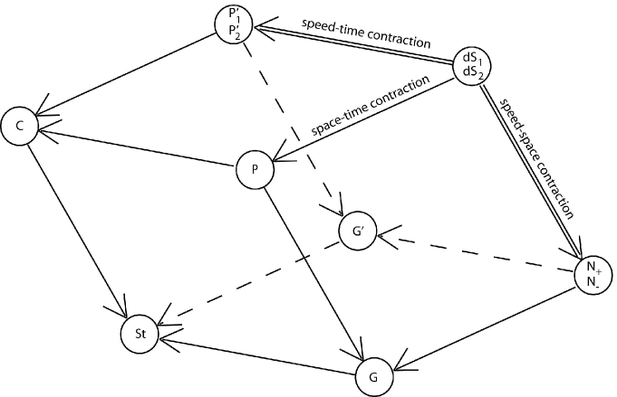
Figure 1: The contractions of the kinematical groups.

The resulting possible Lie algebras give 11 possible kinematics, where each of the kinematical groups (see Table 1) is generated by its inertial transformations as well as its spacetime translations and spatial rotations. These groups consist of the de Sitter groups and their rotation-invariant contractions: the physical nature of a contracted group is determined by the nature of the contraction itself, along with the nature of the parent de Sitter group. Below we will illustrate the nature of these contractions when we look more closely at the simpler case of a 2-dimensional spacetime. For Fig. 1, note that a “upper” face of the cube is transformed under one type of contraction into the opposite face.

Sanjuan [24] noted that the methods employed by Bacry and Lévy-Leblond could be easily applied to 2-dimensional spacetimes: as it is the purpose of this paper to investigate these kinematical Lie algebras and groups through Clifford algebras, we will begin by explicitly classifying all such possible Lie algebras. This section then is a detailed and expository account of certain parts of Bacry, Lévy-Leblond, and Sanjuan’s work.

Let $K$ denote the generator of the inertial transformations, $H$ the generator of time translations, and $P$ the generator of space translations. As space is one-dimensional, space is isotropic. In the following section we will see how to construct, for each possible kinematical structure, a spacetime that is a homogeneous space for its kinematical group, so that basic principle (i) is satisfied.

Now let $\Pi$ and $\Theta$ denote the respective operations of parity and time-reversal: $K$ must be odd under both $\Pi$ and $\Theta$. Our basic principle (ii) requires that the Lie algebra is acted upon by the $\mathbb{Z}_{2}\otimes\mathbb{Z}_{2}$ group of involutions generated by

$$\Pi\,:\,\left(K,H,P\right)\rightarrow\left(-K,H,-P\right)\qquad\mbox{and}\qquad\Theta\,:\,\left(K,H,P\right)\rightarrow\left(-K,-H,P\right).$$

Finally, basic principle (iii) requires that the subgroup generated by $K$ is noncompact, even though we will allow for the universe to be closed, or even for closed time-like worldlines to exist. We do not wish for $e^{0K}=e^{\theta K}$ for some non-zero $\theta$, for then we would find it possible for a boost to be no boost at all!

As each Lie bracket $[K,H]$, $[K,P]$, and $[H,P]$ is invariant under the involutions $\Pi$ and $\Theta$ as well as the involution

$$\Gamma=\Pi\Theta\,:\,\left(K,H,P\right)\rightarrow\left(K,-H,-P\right),$$

we must have that $[K,H]=pP$, $[K,P]=hH$, and $[H,P]=kK$ for some constants $k$, $h$, and $p$. Note that these Lie brackets are also invariant under the symmetries defined by

$$S_{P}:\{K\leftrightarrow H,p\leftrightarrow-p,k\leftrightarrow h\},\qquad S_{H}:\{K\leftrightarrow P,h\leftrightarrow-h,k\leftrightarrow-p\},\qquad\mbox{and}$$

$$S_{K}:\{H\leftrightarrow P,k\leftrightarrow-k,h\leftrightarrow p\},$$

and that the Jacobi identity is automatically satisfied for any triple of elements of the Lie algebra.

Table 2: The 21 kinematical Lie algebras, grouped into 11 essentially distinct types of kinematics.

$P$

$-P$

$P$

$-P$

$P$

$-P$

$0$

$0$

$0$

$0$

$0$

$H$

$-H$

$H$

$-H$

$0$

$0$

$H$

$-H$

$0$

$0$

$0$

$K$

$-K$

$-K$

$K$

$0$

$0$

$0$

$0$

$K$

$-K$

$0$

$0$

$0$

$0$

$0$

$P$

$-P$

$P$

$-P$

$P$

$-P$

$H$

$-H$

$H$

$-H$

$0$

$0$

$0$

$0$

$H$

$-H$

$K$

$-K$

$-K$

$K$

$K$

$-K$

$-K$

$K$

$0$

$0$

Table 3: 6 non-kinematical Lie algebras.

$P$	$-P$		$P$	$-P$		$-P$	$P$
$-H$	$H$		$-H$	$H$		$H$	$-H$
$K$	$-K$		$-K$	$K$		$0$	$0$

We can normalize the constants $k$, $h$, and $p$ by a scale change so that $k,h,p\in\{-1,0,1\}$, taking advantage of the simple form of the Lie brackets for the basis elements $K$, $H$, and $P$. There are then $3^{3}$ possible Lie algebras, which we tabulate in Tables 2 and 3 with columns that have the following form:

$[K,H]$

$[K,P]$

$[H,P]$

Table 4: Some kinematical groups along with their notation and structure constants.

	Anti-de Sitter	Oscillating Newtonian Universe	Para-Minkowski	Minkowski
	0.2ex $adS$	$N_{-}$	$M^{\prime}$	$M$
0.2ex$[K,H]$	$P$	$P$	$0$	$P$
$[K,P]$	$H$	$0$	$H$	$H$
$[H,P]$	$K$	$K$	$K$	$0$

Table 5: Some kinematical groups along with their notation and structure constants.

	de Sitter	Expanding Newtonian Universe	Expanding Minkowski Universe
	$dS$	$N_{+}$	$M_{+}$
0.2ex$[K,H]$	$P$	$P$	$0$
$[K,P]$	$H$	$0$	$H$
$[H,P]$	$-K$	$-K$	$-K$

Table 6: Some kinematical groups along with their notation and structure constants.

	Galilei	Carroll	Static de Sitter Universe	Static Universe
	$G$	$C$	$SdS$	$St$
$[K,H]$	$P$	$0$	$0$	$0$
$[K,P]$	$0$	$H$	$0$	$0$
$[H,P]$	$0$	$0$	$K$	$0$

We also pair each Lie algebra with its image under the isomorphism given by $P\leftrightarrow-P$, $H\leftrightarrow-H$, $K\leftrightarrow-K$, and $[\star,\star\star]\leftrightarrow[\star\star,\star]$, for both Lie algebras then give the same kinematics. There are then 11 essentially distinct kinematics, as illustrated in Table 2. Also (as we shall see in the next section) each of the other 6 Lie algebras (that are given in Table 3) violate the third basic principle, generating a compact group of inertial transformations.

These non-kinematical Lie algebras are the lie algebras for the motion groups for the elliptic, hyperbolic, and Euclidean planes: let us denote these respective groups as $El$, $H$, and $Eu$.

We name the kinematical groups (that are generated by the boosts and translations) in concert with the 4-dimensional case (see Tables 4, 5, and 6). Each of these kinematical groups is either the de Sitter or the anti-de Sitter group, or one of their contractions. We can contract with respect to any subgroup, giving us three fundamental types of contraction: speed-space, speed-time, and space-time contractions, corresponding respectively to contracting to the subgroups generated by $H$, $P$, and $K$.

Speed-space contractions. We make the substitutions $K\rightarrow\epsilon K$ and $P\rightarrow\epsilon P$ into the Lie algebra and then calculate the singular limit of the Lie brackets as $\epsilon\rightarrow 0$. Physically the velocities are small when compared to the speed of light, and the spacelike intervals are small when compared to the timelike intervals. Geometrically we are describing spacetime near a timelike geodesic, as we are contracting to the subgroup that leaves this worldline invariant, and so are passing from relativistic to absolute time. So $adS$ is contracted to $N_{-}$ while $dS$ is contracted to $N_{+}$, for example.

Speed-time contractions. We make the substitutions $K\rightarrow\epsilon K$ and $H\rightarrow\epsilon H$ into the Lie algebra and then calculate the singular limit of the Lie brackets as $\epsilon\rightarrow 0$. Physically the velocities are small when compared to the speed of light, and the timelike intervals are small when compared to the spacelike intervals. Geometrically we are describing spacetime near a spacelike geodesic, as we are contracting to the subgroup that leaves invariant this set of simultaneous events, and so are passing from relativistic to absolute space. Such a spacetime may be of limited physical interest, as we are only considering intervals connecting events that are not causally related.

Space-time contractions. We make the substitutions $P\rightarrow\epsilon P$ and $H\rightarrow\epsilon H$ into the Lie algebra and then calculate the singular limit of the Lie brackets as $\epsilon\rightarrow 0$. Physically the spacelike and timelike intervals are small, but the boosts are not restricted. Geometrically we are describing spacetime near an event, as we are contracting to the subgroup that leaves invariant only this one event, and so we call the corresponding kinematical group a local group as opposed to a cosmological group.

Fig. 2 illustrates several interesting relationships among the kinematical groups. For example, Table 7 gives important classes of kinematical groups, each class corresponding to a face of the figure, that transform to another class in the table under one of the symmetries $S_{H}$, $S_{P}$, or $S_{K}$, provided that certain exclusions are made as outlined in Table 8. The exclusions are necessary under the given symmetries as some kinematical algebras are taken to algebras that are not kinematical.

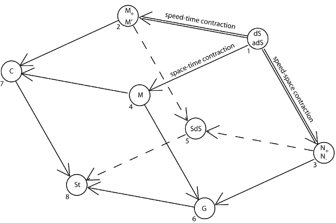
Figure 2: The contractions of the kinematical groups for 2-dimensional spacetimes.

Table 7: Important classes of kinematical groups and their geometrical configurations in Fig. 2.

Class of groups	Face
Relative-time	$1247$
Absolute-time	$3568$
Relative-space	$1346$
Absolute-space	$2578$
Cosmological	$1235$
Local	$4678$

Table 8: The 3 basic symmetries are represented by reflections of Fig. 2, with some exclusions.

Symmetry	Reflection across face
$S_{H}$	$1378$ (excluding $M_{+}$)
$S_{P}$	$1268$ (excluding $adS$ and $N_{-}$)
$S_{K}$	$1458$

2 Cayley–Klein geometries

In this section we wish to review work done by Ballesteros, Herranz, Ortega and Santander on homogeneous spaces that are spacetimes for kinematical groups, and we begin with a bit of history concerning the discovery of non-Euclidean geometries. Franz Taurinus was the first to explicitly give mathematical details on how a hypothetical sphere of imaginary radius would have a non-Euclidean geometry, what he called log-spherical geometry, and this was done via hyperbolic trigonometry (see [6] or [19]). Felix Klein is usually given credit for being the first to give a complete model of a non-Euclidean geometry: he built his model by suitably adapting Arthur Cayley’s metric for the projective plane. Klein [20] (originally published in 1871) went on, in a systematic way, to describe nine types of two-dimensional geometries (what Yaglom [29] calls Cayley–Klein geometries) that were then further investigated by Sommerville [27]. Yaglom gave conformal models for these geometries, extending what had been done for both the projective and hyperbolic planes. Each type of geometry is homogeneous and can be determined by two real constants ${\kappa_{1}}$ and ${\kappa_{2}}$ (see Table 9). The names of the geometries when ${\kappa_{2}}\leq 0$ are those as given by Yaglom, and it is these six geometries that can be interpreted as spacetime geometries.

Table 9: The 9 types of Cayley–Klein geometries.

	Metric Structure
Conformal	Elliptic	Parabolic	Hyperbolic
Structure	${\kappa_{1}}>0$	${\kappa_{1}}=0$	${\kappa_{1}}<0$
1ex Elliptic	elliptic	Euclidean	hyperbolic
${\kappa_{2}}>0$	geometries	geometries	geometries
Parabolic	co-Euclidean	Galilean	co-Minkowski
${\kappa_{2}}=0$	geometries	geometry	geometries
Hyperbolic	co-hyperbolic	Minkowski	doubly
${\kappa_{2}}<0$	geometries	geometries	hyperbolic
			geometries

Following Taurinus, it is easiest to describe a bit of the geometrical nature of these geometries by applying the appropriate kind of trigonometry: we will see shortly how to actually construct a model for each geometry. Let $\kappa$ be a real constant. The unit circle $a^{2}+\kappa b^{2}=1$ in the plane ${\mathbb{R}}^{2}=\{(a,b)\}$ with metric $ds^{2}=da^{2}+\kappa db^{2}$ can be used to defined the cosine

$${C_{\kappa}}(\phi)=\begin{cases}\cos{\left(\sqrt{\kappa}\,\phi\right)},&\text{if $\kappa>0$},\\ 1,&\text{if $\kappa=0$},\\ \cosh{\left(\sqrt{-\kappa}\,\phi\right)},&\text{if $\kappa<0$},\\ \end{cases}$$

and sine

$${S_{\kappa}}(\phi)=\begin{cases}\frac{1}{\sqrt{\kappa}}\sin{\left(\sqrt{\kappa}\,\phi\right)},&\text{if $\kappa>0$},\\ \phi,&\text{if $\kappa=0$},\\ \frac{1}{\sqrt{-\kappa}}\sinh{\left(\sqrt{-\kappa}\,\phi\right)},&\text{if $\kappa<0$}\\ \end{cases}$$

functions: here $(a,b)=({C_{\kappa}}(\phi),{S_{\kappa}}(\phi))$ is a point on the connected component of the unit circle containing the point $(1,0)$, and $\phi$ is the signed distance from $(1,0)$ to $(a,b)$ along the circular arc, defined modulo the length $\dfrac{2\pi}{\sqrt{\kappa}}$ of the unit circle when $\kappa>0$. We can also write down the power series for these analytic trigonometric functions:

$${C_{\kappa}}(\phi)=1-\frac{1}{2!}\kappa\phi^{2}+\frac{1}{4!}\kappa^{2}\phi^{4}+\cdots,$$

$${S_{\kappa}}(\phi)=\phi-\frac{1}{3!}\kappa\phi^{3}+\frac{1}{5!}\kappa^{2}\phi^{5}+\cdots.$$

Note that ${C_{\kappa}}^{2}(\phi)+\kappa{S_{\kappa}}^{2}(\phi)=1$. So if $\kappa>0$ then the unit circle is an ellipse (giving us elliptical trigonometry), while if $\kappa<0$ it is a hyperbola (giving us hyperbolic trigonometry). When $\kappa=0$ the unit circle consists of two parallel straight lines, and we will say that our trigonometry is parabolic. We can use such a trigonometry to define the angle $\phi$ between two lines, and another independently chosen trigonometry to define the distance between two points (as the angle between two lines, where each line passes through one of the points as well as a distinguished point).

At this juncture it is not clear that such geometries, as they have just been described, are of either mathematical or physical interest. That mathematicians and physicists at the beginning of the 20th century were having similar thoughts is perhaps not surprising, and Walker [28] gives an interesting account of the mathematical and physical research into non-Euclidean geometries during this period in history. Klein found that there was a fundamental unity to these geometries, and so that alone made them worth studying. Before we return to physics, let us look at these geometries from a perspective that Klein would have appreciated, describing their motion groups in a unified manner.

Ballesteros, Herranz, Ortega and Santander have constructed the Cayley–Klein geometries as homogeneous spaces by looking at real representations of their motion groups. These motion groups are denoted by ${SO_{{\kappa_{1}},{\kappa_{2}}}(3)}$ (that we will refer to as the generalized $SO(3)$ or simply by $SO(3)$) with their respective Lie algebras being denoted by ${so_{{\kappa_{1}},{\kappa_{2}}}(3)}$ (that we will refer to as the generalized $so(3)$ or simply by $so(3)$), and most if not all of these groups are probably familiar to the reader (for example, if both ${\kappa_{1}}$ and ${\kappa_{2}}$ vanish, then $SO(3)$ is the Heisenberg group). Later on in this paper we will use Clifford algebras to show how we can explicitly think of $SO(3)$ as a rotation group, where each element of $SO(3)$ has a well-defined axis of rotation and rotation angle.

Now a matrix representation of $so(3)$ is given by the matrices

$$H=\left(\begin{matrix}0&-{\kappa_{1}}&0\\ 1&0&0\\ 0&0&0\end{matrix}\right),\qquad P=\left(\begin{matrix}0&0&-{\kappa_{1}}{\kappa_{2}}\\ 0&0&0\\ 1&0&0\end{matrix}\right),\qquad\mbox{and}\qquad K=\left(\begin{matrix}0&0&0\\ 0&0&-{\kappa_{2}}\\ 0&1&0\end{matrix}\right),$$

where the structure constants are given by the commutators

$$\left[K,H\right]=P,\qquad\left[K,P\right]=-{\kappa_{2}}H,\qquad\mbox{and}\qquad\left[H,P\right]={\kappa_{1}}K.$$

By normalizing the constants we obtain matrix representations of the $adS$, $dS$, $N_{-}$, $N_{+}$, $M$, and $G$ Lie algebras, as well as the Lie algebras for the elliptic, Euclidean, and hyperbolic motion groups, denoted $El$, $Eu$, and $H$ respectively. We will see at the end of this section how the Cayley–Klein spaces can also be used to give homogeneous spaces for $M^{\prime}$, $M_{+}$, $C$, and $SdS$ (but not for $St$). One benefit of not normalizing the parameters ${\kappa_{1}}$ and ${\kappa_{2}}$ is that we can easily obtain contractions by letting ${\kappa_{1}}\rightarrow 0$ or ${\kappa_{2}}\rightarrow 0$.

Elements of $SO(3)$ are real-linear, orientation-preserving isometries of ${\mathbb{R}}^{3}=\{(z,t,x))\}$ imbued with the (possibly indefinite or degenerate) metric $ds^{2}=dz^{2}+{\kappa_{1}}dt^{2}+{\kappa_{1}}{\kappa_{2}}dx^{2}$. The one-parameter subgroups $\mathcal{H}$, $\mathcal{P}$, and $\mathcal{K}$ generated respectively by $H$, $P$, and $K$ consist of matrices of the form

$$e^{\alpha H}=\left(\begin{matrix}C_{{\kappa_{1}}}(\alpha)&-{\kappa_{1}}S_{{\kappa_{1}}}(\alpha)&0\\ S_{{\kappa_{1}}}(\alpha)&C_{{\kappa_{1}}}(\alpha)&0\\ 0&0&1\end{matrix}\right),\qquad e^{\beta P}=\left(\begin{matrix}C_{{\kappa_{1}}{\kappa_{2}}}(\beta)&0&-{\kappa_{1}}{\kappa_{2}}S_{{\kappa_{1}}{\kappa_{2}}}(\beta)\\ 0&1&0\\ S_{{\kappa_{1}}{\kappa_{2}}}(\beta)&0&C_{{\kappa_{1}}{\kappa_{2}}}(\beta)\end{matrix}\right),$$

and

$$e^{\theta K}=\left(\begin{matrix}1&0&0\\ 0&C_{{\kappa_{2}}}(\theta)&-{\kappa_{2}}S_{{\kappa_{2}}}(\theta)\\ 0&S_{{\kappa_{2}}}(\theta)&C_{{\kappa_{2}}}(\theta)\end{matrix}\right)$$

(note that the orientations induced on the coordinate planes may be different than expected). We can now see that in order for $\mathcal{K}$ to be non-compact, we must have that ${\kappa_{2}}\leq 0$, which explains the content of Table 3.

The spaces $SO(3)/\mathcal{K}$, $SO(3)/\mathcal{H}$, and $SO(3)/\mathcal{P}$ are homogeneous spaces for $SO(3)$. When $SO(3)$ is a kinematical group, then $S\equiv SO(3)/\mathcal{K}$ can be identified with the manifold of space-time translations. Regardless of the values of ${\kappa_{1}}$ and ${\kappa_{2}}$ however, $S$ is the Cayley–Klein geometry with parameters ${\kappa_{1}}$ and ${\kappa_{2}}$, and $S$ can be shown to have constant curvature ${\kappa_{1}}$ (also, see [21]). So the angle between two lines passing through the origin (the point that is invariant under the subgroup $\mathcal{K}$) is given by the parameter $\theta$ of the element of $\mathcal{K}$ that rotates one line to the other (and so the measure of angles is related to the parameter ${\kappa_{2}}$). Similarly if one point can be taken to another by an element of $\mathcal{H}$ or $\mathcal{P}$ respectively, then the distance between the two points is given by the parameter $\alpha$ or $\beta$, (and so the measure of distance is related to the parameter ${\kappa_{1}}$ or to ${\kappa_{1}}{\kappa_{2}}$). Note that the spaces $SO(3)/\mathcal{H}$ and $SO(3)/\mathcal{P}$ are respectively the spaces of timelike and spacelike geodesics for kinematical groups.

For our purposes we will also need to model $S$ as a projective geometry. First, we define the projective quadric $\bar{\Sigma}$ as the set of points on the unit sphere $\Sigma\equiv\{(z,t,x)\in{\mathbb{R}}^{3}\;|\;z^{2}+{\kappa_{1}}t^{2}+{\kappa_{1}}{\kappa_{2}}x^{2}=1\}$ that have been identified by the equivalence relation $(z,t,x)\thicksim(-z,-t,-x)$. The group $SO(3)$ acts on $\bar{\Sigma}$, and the subgroup $\mathcal{K}$ is then the isotropy subgroup of the equivalence class $\mathcal{O}=[(1,0,0)]$. The metric $g$ on ${\mathbb{R}}^{3}$ induces a metric on $\bar{\Sigma}$ that has ${\kappa_{1}}$ as a factor. If we then define the main metric $g_{1}$ on $\bar{\Sigma}$ by setting

$$\left(ds^{2}\right)_{1}=\frac{1}{{\kappa_{1}}}ds^{2},$$

then the surface $\bar{\Sigma}$, along with its main metric (and subsidiary metric, see below), is a projective model for the Cayley–Klein geometry $S$. Note that in general $g_{1}$ can be indefinite as well as nondegenerate.

The motion $\exp(\theta K$) gives a rotation (or boost for a spacetime) of $S$, whereas the motions $\exp(\alpha H$) and $\exp(\beta P$) give translations of $S$ (time and space translations respectively for a spacetime). The parameters ${\kappa_{1}}$ and ${\kappa_{2}}$ are, for the spacetimes, identified with the universe time radius $\tau$ and speed of light $c$ by the formulae

$${\kappa_{1}}=\pm\frac{1}{\tau^{2}}\qquad\mbox{and}\qquad{\kappa_{2}}=-\frac{1}{c^{2}}.$$

For the absolute-time spacetimes with kinematical groups $N_{-}$, $G$, and $N_{+}$, where ${\kappa_{2}}=0$ and $c=\infty$, we foliate $S$ so that each leaf consists of all points that are simultaneous with one another, and then $SO(3)$ acts transitively on each leaf. We then define the subsidiary metric $g_{2}$ along each leaf of the foliation by setting

$$\left(ds^{2}\right)_{2}=\frac{1}{{\kappa_{2}}}\left(ds^{2}\right)_{1}.$$

Of course when ${\kappa_{2}}\neq 0$, the subsidiary metric can be defined on all of $\bar{\Sigma}$. The group $SO(3)$ acts on $S$ by isometries of $g_{1}$, by isometries of $g_{2}$ when ${\kappa_{2}}\neq 0$ and, when ${\kappa_{2}}=0$, on the leaves of the foliation by isometries of $g_{2}$.

It remains to be seen then how homogeneous spacetimes for the kinematical groups $M_{+},$ $M^{\prime},$ $C,\!$ and $SdS$ may be obtained from the Cayley–Klein geometries. In Fig. 3 the face $1346$ contains the motion groups for all nine types of Cayley–Klein geometries, and the symmetries $S_{H}$, $S_{P}$, and $S_{K}$ can be represented as symmetries of the cube, as indicated in Table 10. As vertices $1$ and $8$ are in each of the three planes of reflection, it is impossible to get $St$ from any one of the Cayley–Klein groups through the symmetries $S_{H}$, $S_{P}$, and $S_{K}$. Under the symmetry $S_{K}$, respective spacetimes for $M_{+}$, $M^{\prime}$, and $C$ are given by the spacetimes $SO(3)/\mathcal{K}$ for $N_{+}$, $N_{-}$, and $G$, where space and time translations are interchanged.

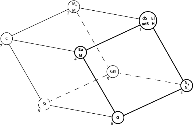
Figure 3: The 9 kinematical and 3 non-kinematical groups.

Table 10: The 3 basic symmetries are given as reflections of Fig. 3.

Symmetry	Reflection across face
$S_{H}$	$1378$
$S_{P}$	$1268$
$S_{K}$	$1458$

Under the symmetry $S_{H}$, the spacetime for $SdS$ is given by the homogeneous space $SO(3)/\mathcal{P}$ for $G$, as boosts and space translations are interchanged by $S_{H}$. Note however that there actually are no spacelike geodesics for $G$, as the Cayley–Klein geometry $S=SO(3)/\mathcal{K}$ for ${\kappa_{1}}={\kappa_{2}}=0$ can be given simply by the plane ${\mathbb{R}}^{2}=\{(t,x)\}$ with $ds^{2}=dt^{2}$ as its line element. Although $SO(3)/\mathcal{P}$ is a homogeneous space for $SO(3)$, $SO(3)$ does not act effectively on $SO(3)/\mathcal{P}$: since both $[K,P]=0$ and $[H,P]=0$, space translations do not act on $SO(3)/\mathcal{P}$. Similarly, inertial transformations do not act on spacetime for $SdS$, or on $St$ for that matter. Note that $SdS$ can be obtained from $dS$ by $P\rightarrow\epsilon P$, $H\rightarrow\epsilon H$, and $K\rightarrow\epsilon^{2}K$, where $\epsilon\rightarrow 0$. So velocities are negligible even when compared to the reduced space and time translations.

In conclusion to Part I then, a study of all nine types of Cayley–Klein geometries affords us a beautiful and unified study of all 11 possible kinematics save one, the static kinematical structure. It was this study that motivated the author to investigate another unified approach to possible kinematics, save for that of the Static Universe.

Part II. Another unified approach to possible kinematics

3 The generalized Lie algebra $\boldsymbol{so(3)}$

Preceding the work of Ballesteros, Herranz, Ortega, and Santander was the work of Sanjuan [24] on possible kinematics and the nine Cayley–Klein geometries. Sanjuan represents each kinematical Lie algebra as a real matrix subalgebra of $M(2,{\mathbb{C}})$, where ${\mathbb{C}}$ denotes the generalized complex numbers (a description of the generalized complex numbers is given below). This is accomplished using Yaglom’s analytic representation of each Caley–Klein geometry as a region of ${\mathbb{C}}$: for the hyperbolic plane this gives the well-known Poincaré disk model. Sanjuan constructs the Lie algebra for the hyperbolic plane using the standard method, stating that this method can be used to obtain the other Lie algebras as well. Also, extensive work has been done by Gromov [7, 8, 9, 10, 11] on the generalized orthogonal groups $SO(3)$ (which we refer to simply as $SO(3)$), deriving representations of the generalized $so(3)$ (which we refer to simply as $so(3)$) by utilizing the dual numbers as well as the standard complex numbers, where again it is tacitly assumed that the parameters ${\kappa_{1}}$ and ${\kappa_{2}}$ have been normalized. Also, Pimenov has given an axiomatic description of all Cayley–Klein spaces in arbitrary dimensions in his paper [23] via the dual numbers $i_{k}$, $k=1,2,\dots$, where $i_{k}i_{m}=i_{m}i_{k}\neq 0$ and $i_{k}^{2}=0$.

Unless stated otherwise, we will not assume that the parameters ${\kappa_{1}}$ and ${\kappa_{2}}$ have been normalized, as we wish to obtain contractions by simply letting ${\kappa_{1}}\rightarrow 0$ or ${\kappa_{2}}\rightarrow 0$. Our goal in this section is to derive representations of $so(3)$ as real subalgebras of $M(2,{\mathbb{C}})$, and in the process give a conformal model of $S$ as a region of the generalized complex plane ${\mathbb{C}}$ along with a hermitian metric, extending what has been done for the projective and hyperbolic planes. We feel that it is worthwhile to write down precisely how these representations are obtained in order that our later construction of a Clifford algebra is more meaningful.

The first step is to represent the generators of $SO(3)$ by Möbius transformations (that is, linear fractional transformations) of an appropriately defined region in the complex number plane ${\mathbb{C}}$, where the points of $S$ are to be identified with this region.

Definition 3.1.

By the complex number plane ${\mathbb{C}}_{\kappa}$ we will mean $\{w=u+iv\,|\,(u,v)\in{\mathbb{R}}^{2}\ \mbox{and}\ i^{2}=-\kappa\}$ where $\kappa$ is a real-valued parameter.

Thus ${\mathbb{C}}_{\kappa}$ refers to the complex numbers, dual numbers, or double numbers when $\kappa$ is normalized to $1$, $0$, or $-1$ respectively (see [29] and [13]). One may check that ${\mathbb{C}}_{\kappa}$ is an associative algebra with a multiplicative unit, but that there are zero divisors when $\kappa\leq 0$. For example, if $\kappa=0$, then $i$ is a zero-divisor. The reader will note below that $\frac{1}{i}$ appears in certain equations, but that these equations can always be rewritten without the appearance of any zero-divisors in a denominator. One can extend ${\mathbb{C}}_{\kappa}$ so that terms like $\frac{1}{i}$ are well-defined (see [29]). It is these zero divisors that play a crucial rule in determining the null-cone structure for those Cayley–Klein geometries that are spacetimes.

Definition 3.2.

Henceforward ${\mathbb{C}}$ will denote ${\mathbb{C}}_{{\kappa_{2}}}$, as it is the parameter ${\kappa_{2}}$ which determines the conformal structure of the Cayley–Klein geometry $S$ with parameters ${\kappa_{1}}$ and ${\kappa_{2}}$.

Theorem 3.3.

The matrices $\frac{i}{2}{\sigma_{1}}$, $\frac{i}{2}{\sigma_{2}}$, and $\frac{1}{2i}{\sigma_{3}}$ are generators for the generalized Lie algebra $so(3)$, where $so(3)$ is represented as a subalgebra of the real matrix algebra $M(2,{\mathbb{C}})$, where

$${\sigma_{1}}=\left(\begin{matrix}1&0\\ 0&-1\end{matrix}\right),\qquad{\sigma_{2}}=\left(\begin{matrix}0&1\\ {\kappa_{1}}&0\end{matrix}\right)\qquad\mbox{and}\qquad{\sigma_{3}}=\left(\begin{matrix}0&i\\ -{\kappa_{1}}i&0\end{matrix}\right).$$

In fact, we will show that $\mathcal{K}$, $\mathcal{H}$, and $\mathcal{P}$ (the subgroups generated respectively by boosts, time and space translations) can be respectively represented by elements of $SL(2,{\mathbb{C}})$ of the form $e^{i\frac{\theta}{2}{\sigma_{1}}}$, $e^{i\frac{\alpha}{2}{\sigma_{2}}}$, and $e^{\frac{\beta}{2i}{\sigma_{3}}}$.

Note that when ${\kappa_{1}}=1$ and ${\kappa_{2}}=1$, we recover the Pauli spin matrices, though my indexing is different, and there is a sign change as well: recall that the Pauli spin matrices are typically given as

$${\sigma_{1}}=\left(\begin{matrix}0&1\\ 1&0\end{matrix}\right),\qquad{\sigma_{2}}=\left(\begin{matrix}0&-i\\ i&0\end{matrix}\right)\qquad\mbox{and}\qquad{\sigma_{3}}=\left(\begin{matrix}1&0\\ 0&-1\end{matrix}\right).$$

We will refer to ${\sigma_{1}}$, ${\sigma_{2}}$, and ${\sigma_{3}}$ as given in the statement of Theorem 1 as the generalized Pauli spin matrices.

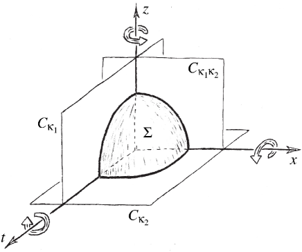
Figure 4: The unit sphere $\Sigma$ and the three complex planes ${\mathbb{C}}_{{\kappa_{2}}}$, ${\mathbb{C}}_{{\kappa_{1}}}$, and ${\mathbb{C}}_{{\kappa_{1}}{\kappa_{2}}}$.

The remainder of this section is devoted to proving the above theorem. The reader may find Fig. 4 helpful. The respective subgroups $\mathcal{K}$, $\mathcal{H}$, and $\mathcal{P}$ preserve the $z$, $x$, and $t$ axes as well as the ${\mathbb{C}}_{{\kappa_{2}}}$, ${\mathbb{C}}_{{\kappa_{1}}}$, and ${\mathbb{C}}_{{\kappa_{1}}{\kappa_{2}}}$ number planes, acting on these planes as rotations. Also, as these groups preserve the unit sphere $\Sigma=\{(z,t,x)\;|\;z^{2}+{\kappa_{1}}t^{2}+{\kappa_{1}}{\kappa_{2}}x^{2}=1\}$, they preserve the respective intersections of $\Sigma$ with the ${\mathbb{C}}_{{\kappa_{2}}}$, ${\mathbb{C}}_{{\kappa_{1}}}$, and ${\mathbb{C}}_{{\kappa_{1}}{\kappa_{2}}}$ number planes. These intersections are, respectively, circles of the form ${\kappa_{1}}w\bar{w}=1$ (there is no intersection when ${\kappa_{1}}=0$ or when ${\kappa_{1}}<0$ and ${\kappa_{2}}>0$), ${\mathsf{w}}\bar{{\mathsf{w}}}=1$, and ${\mathfrak{w}}\bar{{\mathfrak{w}}}=1$, where $w$, ${\mathsf{w}}$, and ${\mathfrak{w}}$ denote elements of ${\mathbb{C}}_{{\kappa_{2}}}$, ${\mathbb{C}}_{{\kappa_{1}}}$, and ${\mathbb{C}}_{{\kappa_{1}}{\kappa_{2}}}$ respectively. We will see in the next section how a general element of $SO(3)$ behaves in a manner similar to the generators of $\mathcal{K}$, $\mathcal{H}$, and $\mathcal{P}$, utilizing the power of a Clifford algebra.

So we will let the plane $z=0$ in ${\mathbb{R}}^{3}$ represent ${\mathbb{C}}$ (recall that ${\mathbb{C}}$ denotes ${\mathbb{C}}_{{\kappa_{2}}}$). We may then identify the points of $S$ with a region $\varsigma$ of ${\mathbb{C}}$ by centrally projecting $\Sigma$ from the point $(-1,0,0)$ onto the plane $z=0$, projecting only those points $(z,t,x)\in\Sigma$ with non-negative $z$-values. The region $\varsigma$ may be open or closed or neither, bounded or unbounded, depending on the geometry of $S$. Such a construction is well known for both the projective and hyperbolic planes ${\bf RP}^{2}$ and ${\bf H}^{2}$ and gives rise to the conformal models of these geometries. We will see later on how the conformal structure on ${\mathbb{C}}$ agrees with that of $S$, and then how the simple hermitian metric (see Appendix B)

$$ds^{2}=\frac{dwd\overline{w}}{\left(1+{\kappa_{1}}\left|w\right|^{2}\right)^{2}}$$

gives the main metric $g_{1}$ for $S$. This metric can be used to help indicate the general character of the region $\varsigma$ for each of the nine types of Cayley–Klein geometries, as illustrated in Fig. 5. Note that antipodal points on the boundary of $\varsigma$ (if there is a boundary) are to be identified. For absolute-time spacetimes (when ${\kappa_{2}}=0$) the subsidiary metric $g_{2}$ is given by

$$g_{2}=\frac{dx^{2}}{\left(1+{\kappa_{1}}t_{0}^{2}\right)^{2}}$$

and is defined on lines $w=t_{0}$ of simultaneous events. For all spacetimes, with Here-Now at the origin, the set of zero-divisors gives the null cone for that event.

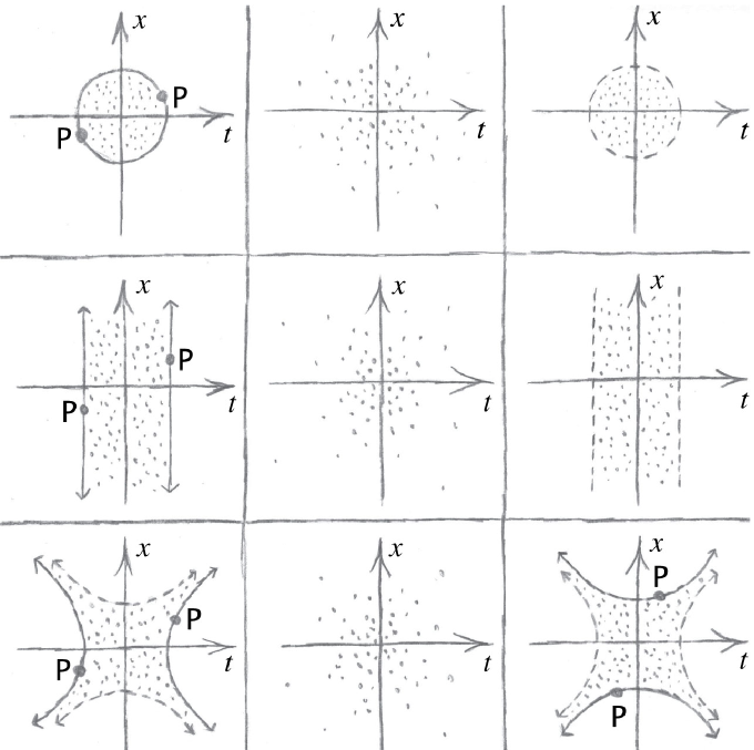
Figure 5: The regions $\varsigma$.

Via this identification of points of $S$ with points of $\varsigma$, transformations of $S$ correspond to transformations of $\varsigma$. If the real parameters ${\kappa_{1}}$ and ${\kappa_{2}}$ are normalized to the values ${K_{1}}$ and ${K_{2}}$ so that

$$K_{i}=\begin{cases}1,&\text{if $\kappa_{i}>0$},\\ 0,&\text{if $\kappa_{i}=0$},\\ -1,&\text{if $\kappa_{i}<0$}\end{cases}$$

then Yaglom [29] has shown that the linear isometries of ${\mathbb{R}}^{3}$ (with metric $ds^{2}=dz^{2}+{K_{1}}dt^{2}+{K_{1}}{K_{2}}dx^{2}$) acting on $\bar{\Sigma}$ project to those Möbius transformations that preserve $\varsigma$, and so these Möbius transformations preserve cycles: a cycle is a curve of constant curvature, corresponding to the intersection of a plane in ${\mathbb{R}}^{3}$ with $\bar{\Sigma}$. We would like to show that elements of $SO(3)$ project to Möbius transformations if the parameters are not normalized, and then to find a realization of $so(3)$ as a real subalgebra of $M(2,{\mathbb{C}})$.

Given ${\kappa_{1}}$ and ${\kappa_{2}}$ we may define a linear isomorphism of ${\mathbb{R}}^{3}$ as indicated below.

${\kappa_{1}}\neq 0,\;{\kappa_{2}}\neq 0$	${\kappa_{1}}\neq 0,\;{\kappa_{2}}=0$	${\kappa_{1}}={\kappa_{2}}=0$
$z\mapsto z^{\prime}=z$	$z\mapsto z^{\prime}=z$	$z\mapsto z^{\prime}=z$
$t\mapsto t^{\prime}=\frac{1}{\sqrt{|{\kappa_{1}}|}}t$	$t\mapsto t^{\prime}=\frac{1}{\sqrt{|{\kappa_{1}}|}}t$	$t\mapsto t^{\prime}=t$
1ex$x\mapsto x^{\prime}=\frac{1}{\sqrt{|{\kappa_{1}}{\kappa_{2}}|}}x$	$x\mapsto x^{\prime}=x$	$x\mapsto x^{\prime}=x$

This transformation preserves the projection point $(-1,0,0)$ as well as the complex plane $z=0$, and maps the projective quadric $\bar{\Sigma}$ for parameters ${K_{1}}$ and ${K_{2}}$ to that for ${\kappa_{1}}$ and ${\kappa_{2}}$, and so gives a correspondence between elements of $SO_{{K_{1}},{K_{2}}}(3)$ with those of ${SO_{{\kappa_{1}},{\kappa_{2}}}(3)}$ as well as the projections of these elements. As the Möbius transformations of ${\mathbb{C}}$ are those transformations that preserve curves of the form

$$\mbox{Im}\frac{(w^{\prime}_{1}-w^{\prime}_{3})(w^{\prime}_{2}-w^{\prime})}{(w^{\prime}_{1}-w^{\prime})(w^{\prime}_{2}-w^{\prime}_{3})}=0$$

(where $w^{\prime}_{1}$, $w^{\prime}_{2}$, and $w^{\prime}_{3}$ are three distinct points lying on the cycle), then if this form is invariant under the induced action of the linear isomorphism, then elements of $SO_{{\kappa_{1}},{\kappa_{2}}}(3)$ project to Möbius transformations of $\varsigma$. As a point $(z,t,x)$ is projected to the point $\left(0,\frac{t}{z+1},\frac{x}{z+1}\right)$ corresponding to the complex number $w=\frac{1}{z+1}(t+\mathcal{I}x)\in{\mathbb{C}}_{{K_{2}}}$, if the linear transformation sends $(z,t,x)$ to $(z^{\prime},t^{\prime},x^{\prime})$, then it sends $w=\frac{1}{z+1}(t+\mathcal{I}x)\in{\mathbb{C}}_{{K_{2}}}$ to $w^{\prime}=\frac{1}{z^{\prime}+1}(t^{\prime}+ix^{\prime})\in{\mathbb{C}}_{{\kappa_{2}}}={\mathbb{C}}$, where $\mathcal{I}^{2}=-{K_{2}}$ and $i^{2}=-{\kappa_{2}}$. We can then write that

${\kappa_{1}}\neq 0,\;{\kappa_{2}}\neq 0$	${\kappa_{1}}\neq 0,\;{\kappa_{2}}=0$	${\kappa_{1}}={\kappa_{2}}=0$
1ex $w=\frac{1}{z+1}\left(t+\mathcal{I}x\right)\mapsto$	$w=\frac{1}{z+1}\left(t+\mathcal{I}x\right)\mapsto$	$w=\frac{1}{z+1}\left(t+\mathcal{I}x\right)\mapsto$
$w^{\prime}=\frac{1}{z+1}\frac{1}{\sqrt{|{\kappa_{1}}|}}\left(t+\frac{\mathcal{I}}{\sqrt{|{\kappa_{2}}|}}x\right)$	$w^{\prime}=\frac{1}{z+1}\left(\frac{1}{\sqrt{|{\kappa_{1}}|}}t+\mathcal{I}x\right)$	$w^{\prime}=w$ 1ex

And so

$$\mbox{Im}\frac{(w_{1}-w_{3})(w_{2}-w)}{(w_{1}-w)(w_{2}-w_{3})}=0\iff\mbox{Im}\frac{(w^{\prime}_{1}-w^{\prime}_{3})(w^{\prime}_{2}-w^{\prime})}{(w^{\prime}_{1}-w^{\prime})(w^{\prime}_{2}-w^{\prime}_{3})}=0,$$

as can be checked directly, and we then have that elements of $SO(3)$ project to Möbius transformations of $\varsigma$.

The rotations $e^{\theta K}$ preserve the complex number plane $z=t+ix=0$ and so correspond simply to the transformations of ${\mathbb{C}}$ given by $w\mapsto e^{i\theta}w$, as $e^{i\theta}={C_{{\kappa_{2}}}}(\theta)+i{S_{{\kappa_{2}}}}(\theta)$, keeping in mind that $i^{2}=-{\kappa_{2}}$. Now in order to express this rotation as a Möbius transformation, we can write

$$w\mapsto\frac{e^{\frac{\theta}{2}i}w+0}{0w+e^{-\frac{\theta}{2}i}}.$$

Since there is a group homomorphism from the subgroup of Möbius transformations corresponding to $SO(3)$ to the group $M(2,{\mathbb{C}})$ of $2\times 2$ matrices with entries in ${\mathbb{C}}$, this transformation being defined by

$$\frac{aw+b}{cw+d}\mapsto\left(\begin{matrix}a&b\\ c&d\end{matrix}\right),$$

each Möbius transformation is covered by two elements of $SL(2,{\mathbb{C}})$. So the rotations $e^{\theta K}$ correspond to the matrices

$$\pm\left(\begin{matrix}e^{\frac{\theta}{2}i}&0\\ 0&e^{-\frac{\theta}{2}i}\end{matrix}\right)=\pm e^{\frac{\theta}{2}i\left(\begin{matrix}1&0\\ 0&-1\end{matrix}\right).}$$

For future reference let us now define

$${\sigma_{1}}\equiv\left(\begin{matrix}1&0\\ 0&-1\end{matrix}\right),$$

where $\frac{i}{2}{\sigma_{1}}$ is then an element of the Lie algebra $so(3)$.

We now wish to see which elements of $SL(2,{\mathbb{C}})$ correspond to the motions $e^{\alpha H}$ and $e^{\beta P}$. The $x$-axis, the $zt$-coordinate plane, and the unit sphere $\Sigma$, are all preserved by $e^{\alpha H}$. So the $zt$-coordinate plane is given the complex structure ${{\mathbb{C}}_{{\kappa_{1}}}}=\{{\mathsf{w}}=z+it\,|\,i^{2}=-{\kappa_{1}}\}$, for then the unit circle ${\mathsf{w}}\overline{{\mathsf{w}}}=1$ gives the intersection of $\Sigma$ with ${{\mathbb{C}}_{{\kappa_{1}}}}$, and the transformation induced on ${{\mathbb{C}}_{{\kappa_{1}}}}$ by $e^{\alpha H}$ is simply given by ${\mathsf{w}}\mapsto e^{i\alpha}{\mathsf{w}}$. Similarly the transformation induced by $e^{\beta P}$ on ${{\mathbb{C}}_{{\kappa_{1}}{\kappa_{2}}}}=\{{\mathfrak{w}}=z+ix\;|\;i^{2}=-{\kappa_{1}}{\kappa_{2}}\}$ is given by ${\mathfrak{w}}\mapsto e^{i\beta}{\mathfrak{w}}$.

In order to explicitly determine the projection of the rotation ${\mathsf{w}}\mapsto e^{i\alpha}{\mathsf{w}}$ of the unit circle in ${{\mathbb{C}}_{{\kappa_{1}}}}$ and also that of the rotation ${\mathfrak{w}}\mapsto e^{i\beta}{\mathfrak{w}}$ of the unit circle in ${{\mathbb{C}}_{{\kappa_{1}}{\kappa_{2}}}}$, note that the projection point $(z,t,x)=(-1,0,0)$ lies in either unit circle and that projection sends a point on the unit circle (save for the projection point itself) to a point on the imaginary axis as follows:

$${\mathsf{w}}=e^{i\phi}\mapsto i{T_{{\kappa_{1}}}}\left(\frac{\phi}{2}\right),\qquad{\mathfrak{w}}=e^{i\phi}\mapsto i{T_{{\kappa_{1}}{\kappa_{2}}}}\left(\frac{\phi}{2}\right)$$

(where $T_{\kappa}$ is the tangent function) for

$$T_{\kappa}\left(\frac{\mu}{2}\right)=\frac{S_{\kappa}(\mu)}{C_{\kappa}(\mu)+1},$$

noting that a point $a+ib$ on the unit circle $w\overline{w}$ of the complex plane $C_{\kappa}$ can be written as $a+ib=e^{i\psi}={C_{\kappa}}(\psi)+i{S_{\kappa}}(\psi)$. So the rotations $e^{\alpha H}$ and $e^{\beta P}$ induce the respective transformations

$$i{T_{{\kappa_{1}}}}\left(\frac{\phi}{2}\right)\mapsto i{T_{{\kappa_{1}}}}\left(\frac{\phi+\alpha}{2}\right),\qquad i{T_{{\kappa_{1}}{\kappa_{2}}}}\left(\frac{\phi}{2}\right)\mapsto i{T_{{\kappa_{1}}{\kappa_{2}}}}\left(\frac{\phi+\beta}{2}\right)$$

on the imaginary axes. We know that such transformations of either imaginary or real axes can be extended to Möbius transformations, and in fact uniquely determine such Möbius maps. For example, if ${\mathsf{w}}=i{T_{{\kappa_{1}}}}\left(\frac{\phi}{2}\right)$, then we have that

$${\mathsf{w}}\mapsto\frac{{\mathsf{w}}+i{T_{{\kappa_{1}}}}\left(\frac{\alpha}{2}\right)}{1-\frac{{\kappa_{1}}{\mathsf{w}}}{i}{T_{{\kappa_{1}}}}\left(\frac{\alpha}{2}\right)}$$

or

$${\mathsf{w}}\mapsto\frac{{C_{{\kappa_{1}}}}\left(\frac{\alpha}{2}\right){\mathsf{w}}+i{S_{{\kappa_{1}}}}\left(\frac{\alpha}{2}\right)}{-\frac{{\kappa_{1}}}{i}{S_{{\kappa_{1}}}}\left(\frac{\alpha}{2}\right){\mathsf{w}}+{C_{{\kappa_{1}}}}\left(\frac{\alpha}{2}\right)}$$

with corresponding matrix representation

$$\pm\left(\begin{matrix}{C_{{\kappa_{1}}}}\left(\frac{\alpha}{2}\right)&i{S_{{\kappa_{1}}}}\left(\frac{\alpha}{2}\right)\vspace{1mm}\\ i{S_{{\kappa_{1}}}}\left(\frac{\alpha}{2}\right)&{C_{{\kappa_{1}}}}\left(\frac{\alpha}{2}\right)\end{matrix}\right)$$

in $SL(2,{C_{{\kappa_{1}}}})$, where we have applied the trigonometric identity

$$T_{\kappa}(\mu\pm\psi)=\frac{T_{\kappa}(\mu)\pm T_{\kappa}(\psi)}{1\mp\kappa T_{\kappa}(\mu)T_{\kappa}(\psi)}.$$

However, it is not these Möbius transformations that we are after, but those corresponding transformations of ${\mathbb{C}}$.

Now a transformation of the imaginary axis (the $x$-axis) of ${{\mathbb{C}}_{{\kappa_{1}}{\kappa_{2}}}}$ corresponds to a transformation of the imaginary axis of ${\mathbb{C}}$ (also the $x$-axis) while a transformation of the imaginary axis of ${{\mathbb{C}}_{{\kappa_{1}}}}$ (the $t$-axis) corresponds to a transformation of the real axis of ${\mathbb{C}}$ (also the $t$-axis). For this reason, values on the $x$-axis, which are imaginary for both the ${\mathbb{C}}_{{\kappa_{1}}{\kappa_{2}}}$ as well as the ${\mathbb{C}}$ plane, correspond as

$$i{T_{{\kappa_{1}}{\kappa_{2}}}}\left(\frac{\phi}{2}\right)=i\frac{1}{\sqrt{{\kappa_{1}}}}{T_{{\kappa_{2}}}}\left(\sqrt{{\kappa_{1}}}\frac{\phi}{2}\right)$$

if ${\kappa_{1}}>0$,

$$i{T_{{\kappa_{1}}{\kappa_{2}}}}\left(\frac{\phi}{2}\right)=i\frac{1}{\sqrt{-{\kappa_{1}}}}T_{-{\kappa_{2}}}\left(\sqrt{-{\kappa_{1}}}\frac{\phi}{2}\right)$$

if ${\kappa_{1}}<0$, and

$$i{T_{{\kappa_{1}}{\kappa_{2}}}}\left(\frac{\phi}{2}\right)=i\left(\frac{\phi}{2}\right)$$

if ${\kappa_{1}}=0$, as can be seen by examining the power series representation for $T_{\kappa}$. The situation for the rotation $e^{i\alpha}$ is similar. We can then compute the elements of $SL(2,{\mathbb{C}})$ corresponding to $e^{\alpha H}$ and $e^{\beta P}$ as given in tables $13$ and $14$ in Appendix C. In all cases we have the simple result that those elements of $SL(2,{\mathbb{C}})$ corresponding to $e^{\alpha H}$ can be written as $e^{\frac{\alpha}{2i}{\sigma_{3}}}$ and those for $e^{\beta P}$ as $e^{i\frac{\beta}{2}{\sigma_{2}}}$, where

$${\sigma_{2}}\equiv\left(\begin{matrix}0&1\\ {\kappa_{1}}&0\end{matrix}\right)\qquad\mbox{and}\qquad{\sigma_{3}}\equiv\left(\begin{matrix}0&i\\ -{\kappa_{1}}i&0\end{matrix}\right).$$

Thus $\frac{i}{2}{\sigma_{1}}$, $\frac{i}{2}{\sigma_{2}}$, and $\frac{1}{2i}{\sigma_{3}}$ are generators for the generalized Lie algebra $so(3)$, a subalgebra of the real matrix algebra $M(2,{\mathbb{C}})$.

4 The Clifford algebra $\boldsymbol{Cl_{3}}$

Definition 4.1.

Let $Cl_{3}$ be the 8-dimensional real Clifford algebra that is identified with $M(2,{\mathbb{C}})$ as indicated by Table 11, where ${\mathbb{C}}$ denotes the generalized complex numbers ${\mathbb{C}}_{{\kappa_{2}}}$. Here we identify the scalar $1$ with the identity matrix and the volume element $i$ with the $2\times 2$ identity matrix multiplied by the complex scalar $i$: in this case $\frac{1}{i}{\sigma_{3}}$ can be thought of as the $2\times 2$ matrix $\left(\begin{matrix}0&1\\ -{\kappa_{1}}&0\end{matrix}\right)$. We will also identify the generalized Paul spin matrices ${\sigma_{1}}$, ${\sigma_{2}}$, and ${\sigma_{3}}$ with the vectors $\hat{i}=\langle 1,0,0\rangle$, $\hat{j}=\langle 0,1,0\rangle$, and $\hat{k}=\langle 0,0,1\rangle$ respectively of the vector space ${\mathbb{R}}^{3}=\{(z,t,x)\}$ given the Cayley–Klein inner product.

Table 11: The basis elements for $Cl_{3}$.

Subspace of		with basis
scalars	${\mathbb{R}}$	1
vectors	${\mathbb{R}}^{3}$	${\sigma_{1}},{\sigma_{2}},{\sigma_{3}}$
bivectors	$\bigwedge^{2}{\mathbb{R}}^{3}$	$i{\sigma_{1}},i{\sigma_{2}},\frac{1}{i}{\sigma_{3}}$
volume elements	$\bigwedge^{3}{\mathbb{R}}^{3}$	$i$

Proposition 4.2.

Let $Cl_{3}$ be the Clifford algebra given by Definition 3.

• The Clifford product $\sigma_{i}^{2}$ gives the square of the length of the vector $\sigma_{i}$ under the Cayley–Klein inner product.

• The center Cen($Cl_{3}$) of $Cl_{3}$ is given by ${\mathbb{R}}\oplus\bigwedge^{3}{\mathbb{R}}^{3}$, the subspace of scalars and volume elements.

• The generalized Lie algebra $so(3)$ is isomorphic to the space of bivectors $\bigwedge^{2}{\mathbb{R}}^{3}$, where

  $$H=\frac{1}{2i}{\sigma_{3}},\qquad P=\frac{i}{2}{\sigma_{2}},\qquad\mbox{and}\qquad K=\frac{i}{2}{\sigma_{1}}.$$

• If $\hat{n}=\langle n^{1},n^{2},n^{3}\rangle$ and $\vec{\sigma}=\langle i{\sigma_{1}},i{\sigma_{2}},{\sigma_{3}}/i\rangle$, then we will let ${\hat{n}\cdot\vec{\sigma}}$ denote the bivector $n^{1}i{\sigma_{1}}+n^{2}i{\sigma_{2}}+n^{3}\frac{1}{i}{\sigma_{3}}$. This bivector is simple, and the parallel vectors $i{\hat{n}\cdot\vec{\sigma}}$ and $\frac{1}{i}{\hat{n}\cdot\vec{\sigma}}$ are perpendicular to any plane element represented by ${\hat{n}\cdot\vec{\sigma}}$. Let $\eta$ denote the line through the origin that is determined by $i{\hat{n}\cdot\vec{\sigma}}$ or $\frac{1}{i}{\hat{n}\cdot\vec{\sigma}}$.

• The generalized Lie group $SO(3)$ is also represented within $Cl_{3}$, for if $a$ is the vector $a^{1}{\sigma_{1}}+a^{2}{\sigma_{2}}+a^{3}{\sigma_{3}}$, then the linear transformation of ${\mathbb{R}}^{3}$ defined by the inner automorphism

  $$a\mapsto e^{-\frac{\phi}{2}\hat{n}\cdot\vec{\sigma}}a\,e^{\frac{\phi}{2}\hat{n}\cdot\vec{\sigma}}$$

  faithfully represents an element of $SO(3)$ as it preserves vector lengths given by the Cayley–Klein inner product, and is in fact a rotation, rotating the vector $\langle a^{1},a^{2},a^{3}\rangle$ about the axis $\eta$ through the angle $\phi$. In this way we see that the spin group is generated by the elements

  $$e^{\frac{\theta}{2}i{\sigma_{1}}},\qquad e^{\frac{\beta}{2}i{\sigma_{2}}},\qquad\mbox{and}\qquad e^{\frac{\alpha}{2i}{\sigma_{3}}}.$$

• Bivectors ${\hat{n}\cdot\vec{\sigma}}$ act as imaginary units as well as generators of rotations in the oriented planes they represent. Let $\varkappa$ be the scalar $-\left({\hat{n}\cdot\vec{\sigma}}\right)^{2}$. Then if $a$ lies in an oriented plane determined by the bivector ${\hat{n}\cdot\vec{\sigma}}$, where this plane is given the complex structure of ${\mathbb{C}}_{\varkappa}$, then $e^{-\frac{\phi}{2}{\hat{n}\cdot\vec{\sigma}}}ae^{\frac{\phi}{2}{\hat{n}\cdot\vec{\sigma}}}$ is simply the vector $\langle a^{1},a^{2},a^{3}\rangle$ rotated by the angle $\phi$ in the complex plane ${\mathbb{C}}_{\varkappa}$, where $\iota^{2}=-\varkappa$. So this rotation is given by unit complex multiplication.

The goal of this section is to prove Proposition 1. We can easily compute the following:

$${\sigma_{1}}^{2}=1,\qquad{\sigma_{2}}^{2}={\kappa_{1}},\qquad{\sigma_{3}}^{2}={\kappa_{1}}{\kappa_{2}},$$

$${\sigma_{3}}{\sigma_{2}}=-{\sigma_{2}}{\sigma_{3}}={\kappa_{1}}i{\sigma_{1}},\qquad{\sigma_{1}}{\sigma_{3}}=-{\sigma_{3}}{\sigma_{1}}=i{\sigma_{2}},$$

$${\sigma_{1}}{\sigma_{2}}=-{\sigma_{2}}{\sigma_{1}}=\frac{1}{i}{\sigma_{3}},\qquad{\sigma_{1}}{\sigma_{2}}{\sigma_{3}}=-{\kappa_{1}}i.$$

Recalling that ${\mathbb{R}}^{3}$ is given the Cayley–Klein inner product, we see that $\sigma_{i}^{2}$ gives the square of the length of the vector $\sigma_{i}$. Note that when ${\kappa_{1}}=0$, $Cl_{3}$ is not generated by the vectors. Cen($Cl_{3}$) of $Cl_{3}$ is given by ${\mathbb{R}}\oplus\bigwedge^{3}{\mathbb{R}}^{3}$, and we can check directly that if

$$H\equiv\frac{1}{2i}{\sigma_{3}},\qquad P\equiv\frac{i}{2}{\sigma_{2}},\qquad\mbox{and}\qquad K\equiv\frac{i}{2}{\sigma_{1}},$$

then we have the following commutators:

$$\left[H,P\right]=HP-PH=\frac{1}{4}\left({\sigma_{3}}{\sigma_{2}}-{\sigma_{2}}{\sigma_{3}}\right)=\frac{{\kappa_{1}}i{\sigma_{1}}}{2}={\kappa_{1}}K,$$

$$\left[K,H\right]=KH-HK=\frac{1}{4}\left({\sigma_{1}}{\sigma_{3}}-{\sigma_{3}}{\sigma_{1}}\right)=\frac{i{\sigma_{2}}}{2}=P,$$

$$\left[K,P\right]=KP-PK=\frac{i^{2}}{4}\left({\sigma_{1}}{\sigma_{2}}-{\sigma_{2}}{\sigma_{1}}\right)=\frac{i{\sigma_{3}}}{2}=-{\kappa_{2}}H.$$

So the Lie algebra $so(3)$ is isomorphic to the space of bivectors $\bigwedge^{2}{\mathbb{R}}^{3}$.

The product of two vectors $a=a^{1}{\sigma_{1}}+a^{2}{\sigma_{2}}+a^{3}{\sigma_{3}}$ and $b=b^{1}{\sigma_{1}}+b^{2}{\sigma_{2}}+b^{3}{\sigma_{3}}$ in $Cl_{3}$ can be expressed as $ab=a\cdot b+a\wedge b=\frac{1}{2}(ab+ba)+\frac{1}{2}(ab-ba)$, where $a\cdot b=\frac{1}{2}(ab+ba)=a^{1}b^{1}+{\kappa_{1}}a^{2}b^{2}+{\kappa_{1}}{\kappa_{2}}a^{3}b^{3}$ is the Cayley–Klein inner product and the wedge product is given by

$$a\wedge b=\frac{1}{2}(ab-ba)=\left|\begin{matrix}-{\kappa_{1}}i{\sigma_{1}}&-i{\sigma_{2}}&\frac{1}{i}{\sigma_{3}}\\ a^{1}&a^{2}&a^{3}\\ b^{1}&b^{2}&b^{3}\end{matrix}\right|,$$

so that $ab$ is the sum of a scalar and a bivector: here $|\star|$ denotes the usual $3\times 3$ determinant.

By the properties of the determinant, if $e\wedge f=g\wedge h$ and ${\kappa_{1}}\neq 0$, then the vectors $e$ and $f$ span the same oriented plane as the vectors $g$ and $h$. When ${\kappa_{1}}=0$ the bivector ${\hat{n}\cdot\vec{\sigma}}$ is no longer simple in the usual way. For example, for the Galilean kinematical group (aka the Heisenberg group) where ${\kappa_{1}}=0$ and ${\kappa_{2}}=0$, we have that both ${\sigma_{1}}\wedge{\sigma_{3}}=i{\sigma_{2}}$ and $\left({\sigma_{1}}+{\sigma_{2}}\right)\wedge{\sigma_{3}}=i{\sigma_{2}}$, so that the bivector $i{\sigma_{2}}$ represents plane elements that do no all lie in the same plane. Recalling that ${\sigma_{1}}$, ${\sigma_{2}}$, and ${\sigma_{3}}$ correspond to the vectors $\hat{i}$, $\hat{j}$, and $\hat{k}$ respectively, we observe that the subgroup $\mathcal{P}$ of the Galilean group fixes the $t$-axis and preserves both of these planes, inducing the same kind of rotation upon each of them: for the plane spanned by $\hat{i}$ and $\hat{k}$ we have that

$$e^{\beta P}:\left(\begin{matrix}\hat{i}\\ \hat{k}\end{matrix}\right)\mapsto\left(\begin{matrix}\hat{i}+\beta\hat{k}\\ \hat{k}\end{matrix}\right)$$

while for the plane spanned by $\hat{i}+\hat{j}$ and $\hat{k}$ we have that

$$e^{\beta P}:\left(\begin{matrix}\hat{i}+\hat{j}\\ \hat{k}\end{matrix}\right)\mapsto\left(\begin{matrix}\hat{i}+\hat{j}+\beta\hat{k}\\ \hat{k}\end{matrix}\right).$$

If we give either plane the complex structure of the dual numbers so that $i^{2}=0$, then the rotation is given by simply multiplying vectors in the plane by the unit complex number $e^{\beta i}$. We will see below that this kind of construction holds generally.

What we need for our construction below is that any bivector can be meaningfully expressed as $e\wedge f$ for some vectors $e$ and $f$, so that the bivector represents at least one plane element: we will discuss the meaning of the magnitude and orientation of the plane element at the end of the section. If the bivector represents multiple plane elements spanning distinct planes, so much the better. If $\hat{n}=\langle n^{1},n^{2},n^{3}\rangle$ and $\vec{\sigma}=\langle i{\sigma_{1}},i{\sigma_{2}},{\sigma_{3}}/i\rangle$, then we will let ${\hat{n}\cdot\vec{\sigma}}$ denote the bivector $B=n^{1}i{\sigma_{1}}+n^{2}i{\sigma_{2}}+n^{3}\frac{1}{i}{\sigma_{3}}$. Now if

$$a=n^{1}{\sigma_{3}}+{\kappa_{1}}n^{3}{\sigma_{1}},\qquad b=-n^{1}{\sigma_{2}}+{\kappa_{1}}n^{2}{\sigma_{1}},\qquad c=n^{3}{\sigma_{2}}+n^{2}{\sigma_{3}},$$

then

$$a\wedge c={\kappa_{1}}n^{3}{\hat{n}\cdot\vec{\sigma}},\qquad b\wedge a={\kappa_{1}}n^{1}{\hat{n}\cdot\vec{\sigma}},\qquad b\wedge c={\kappa_{1}}n^{2}{\hat{n}\cdot\vec{\sigma}},$$

where at least one of the bivectors $n^{i}{\hat{n}\cdot\vec{\sigma}}$ is non-zero as ${\hat{n}\cdot\vec{\sigma}}$ is non-zero. If ${\kappa_{1}}=0$ and $n^{1}=0$, then ${\sigma_{1}}\wedge c={\hat{n}\cdot\vec{\sigma}}$. However, if both ${\kappa_{1}}=0$ and $n^{1}\neq 0$, then it is impossible to have $e\wedge f={\hat{n}\cdot\vec{\sigma}}$: in this context we may simply replace the expression ${\hat{n}\cdot\vec{\sigma}}$ with the expression ${\sigma_{3}}\wedge{\sigma_{2}}$ whenever ${\kappa_{1}}=0$ and $n^{1}\neq 0$ (as we will see at the end of this section, we could just as well replace ${\hat{n}\cdot\vec{\sigma}}$ with any non-zero multiple of ${\sigma_{3}}\wedge{\sigma_{2}}$). The justification for this is given by letting ${\kappa_{1}}\rightarrow 0$, for then

$$e\wedge f=\left(\sqrt{|{\kappa_{1}}|}n^{2}{\sigma_{1}}-\frac{n^{1}}{\sqrt{|{\kappa_{1}}|}}{\sigma_{2}}\right)\wedge\left(\sqrt{|{\kappa_{1}}|}\frac{n^{3}}{n^{1}}{\sigma_{1}}+\frac{1}{\sqrt{|{\kappa_{1}}|}}{\sigma_{3}}\right)={\hat{n}\cdot\vec{\sigma}}$$

shows that the plane spanned by the vectors $e$ and $f$ tends to the $xt$-coordinate plane. We will see below how each bivector ${\hat{n}\cdot\vec{\sigma}}$ corresponds to an element of $SO(3)$ that preserves any oriented plane corresponding to ${\hat{n}\cdot\vec{\sigma}}$: in the case where ${\kappa_{1}}=0$ and $n^{1}\neq 0$, we will then have that this element preserves the $tx$-coordinate plane, which is all that we require.

It is interesting to note that the parallel vectors $i(a\wedge b)$ and $\frac{1}{i}(a\wedge b)$ (when defined) are perpendicular to both $a$ and $b$ with respect to the Cayley–Klein inner product, as can be checked directly. However, due to the possible degeneracy of the Cayley–Klein inner product, there may not be a unique direction that is perpendicular to any given plane. The vector $i{\hat{n}\cdot\vec{\sigma}}=-{\kappa_{2}}n^{1}{\sigma_{1}}-{\kappa_{2}}n^{2}{\sigma_{2}}+n^{3}{\sigma_{1}}$ is non-zero and perpendicular to any plane element corresponding to ${\hat{n}\cdot\vec{\sigma}}$ except when both ${\kappa_{2}}=0$ and $n^{3}=0$, in which case $i{\hat{n}\cdot\vec{\sigma}}$ is the zero vector. In this last case the vector $\frac{1}{i}{\hat{n}\cdot\vec{\sigma}}=n^{1}{\sigma_{1}}+n^{2}{\sigma_{2}}$ gives a non-zero normal vector. In either case, let $\eta$ denote the axis through the origin that contains either of these normal vectors.

Before we continue, let us reexamine those elements of $SO(3)$ that generate the subgroups $\mathcal{K}$, $\mathcal{P}$, and $\mathcal{H}$. Here the respective axes of rotation (parallel to ${\sigma_{1}}$, ${\sigma_{2}}$, and ${\sigma_{3}}$) for the generators $e^{\theta K}$, $e^{\beta P}$, and $e^{\alpha H}$ are given by $\eta$, where ${\hat{n}\cdot\vec{\sigma}}$ is given by $i{\sigma_{1}}$ (or ${\sigma_{3}}\wedge{\sigma_{2}}$ by convention), $i{\sigma_{2}}={\sigma_{1}}\wedge{\sigma_{3}}$, and $\frac{1}{i}{\sigma_{3}}={\sigma_{1}}\wedge{\sigma_{2}}$. These plane elements are preserved under the respective rotations. In fact, for each of these planes the rotations are given simply by multiplication by a unit complex number, as the $zt$-coordinate plane is identified with ${{\mathbb{C}}_{{\kappa_{1}}}}$, the $zx$-coordinate plane with ${{\mathbb{C}}_{{\kappa_{1}}{\kappa_{2}}}}$, and the $tx$-coordinate plane with ${{\mathbb{C}}_{{\kappa_{2}}}}$ as indicated in Fig. 4. Note that the basis bivectors act as imaginary units in $Cl_{3}$ since

$$\left(\frac{1}{i}{\sigma_{3}}\right)^{2}=-{\kappa_{1}},\qquad\left(i{\sigma_{2}}\right)^{2}=-{\kappa_{1}}{\kappa_{2}},\qquad\mbox{and}\qquad\left(i{\sigma_{1}}\right)^{2}=-{\kappa_{2}}.$$

The product of a vector $a$ and a bivector $B$ can be written as $aB=a\dashv B+a\wedge B=\frac{1}{2}(aB-Ba)+\frac{1}{2}(aB+Ba)$ so that $aB$ is the sum of a vector $a\dashv B$ (the left contraction of $a$ by $B$) and a volume element $a\wedge B$. Let $B=b\wedge c$ for some vectors $b$ and $c$. Then

$$2a\dashv(b\wedge c)=a(b\wedge c)-(b\wedge c)a=\frac{1}{2}a(bc-cb)-\frac{1}{2}(bc-cb)a$$

so that

$$4a\dashv(b\wedge c)=cba+abc-acb-bca$$

$$\phantom{4a\dashv(b\wedge c)}{}=c(b\cdot a+b\wedge a)+(a\cdot b+a\wedge b)c-(a\cdot c+a\wedge c)b-b(c\cdot a+c\wedge a)$$

$$\phantom{4a\dashv(b\wedge c)}{}=2(b\cdot a)c-2(c\cdot a)b+c(b\wedge a)+(a\wedge b)c-(a\wedge c)b-b(c\wedge a)$$

$$\phantom{4a\dashv(b\wedge c)}{}=2(b\cdot a)c-2(c\cdot a)b+c(b\wedge a)-(b\wedge a)c+b(a\wedge c)-(a\wedge c)b$$

$$\phantom{4a\dashv(b\wedge c)}{}=2(b\cdot a)c-2(c\cdot a)b+2\left[c\dashv(b\wedge a)+b\dashv(a\wedge c)\right]$$

$$\phantom{4a\dashv(b\wedge c)}{}=2(b\cdot a)c-2(c\cdot a)b-2a\dashv(c\wedge b)$$

$$\phantom{4a\dashv(b\wedge c)}{}=2(b\cdot a)c-2(c\cdot a)b+2a\dashv(b\wedge c)$$

where we have used the Jacobi identity

$$c\dashv(b\wedge a)+b\dashv(a\wedge c)+a\dashv(c\wedge b)=0,$$

recalling that $M(2,{\mathbb{C}})$ is a matrix algebra where the commutator is given by left contraction. Thus

$$2a\dashv(b\wedge c)=2(b\cdot a)c-2(c\cdot a)b$$

and so

$$a\dashv(b\wedge c)=(a\cdot b)c-(a\cdot c)b.$$

So the vector $a\dashv B$ lies in the plane determined by the plane element $b\wedge c$. Because of the possible degeneracy of the Cayley–Klein metric, it is possible for a non-zero vector $b$ that $b\dashv(b\wedge c)=0$.

We will show that if $a$ is the vector $a^{1}{\sigma_{1}}+a^{2}{\sigma_{2}}+a^{3}{\sigma_{3}}$, then the linear transformation of ${\mathbb{R}}^{3}$ defined by

$$a\mapsto e^{-\frac{\phi}{2}\hat{n}\cdot\vec{\sigma}}a\,e^{\frac{\phi}{2}\hat{n}\cdot\vec{\sigma}}$$

faithfully represents an element of $SO(3)$ (and all elements are thus represented). In this way we see that the spin group is generated by the elements

$$e^{\frac{\theta}{2}i{\sigma_{1}}},e^{\frac{\beta}{2}i{\sigma_{2}}},\qquad\mbox{and}\qquad e^{\frac{\alpha}{2i}{\sigma_{3}}}.$$

First, let us see how, using this construction, the vectors ${\sigma_{1}}$, ${\sigma_{2}}$, and ${\sigma_{3}}$ (and hence the bivectors $i{\sigma_{1}}$, $i{\sigma_{2}}$, and $\frac{1}{i}{\sigma_{3}}$) correspond to rotations of the coordinate axes (and hence coordinate planes) given by $e^{\theta K}$, $e^{\beta P}$, and $e^{\alpha H}$ respectively. Since

$$e^{\frac{\theta}{2}i{\sigma_{1}}}={C_{{\kappa_{2}}}}\left(\frac{\theta}{2}\right)+i{S_{{\kappa_{2}}}}\left(\frac{\theta}{2}\right){\sigma_{1}},\qquad e^{\frac{\beta}{2}i{\sigma_{2}}}={C_{{\kappa_{1}}{\kappa_{2}}}}\left(\frac{\beta}{2}\right)+i{S_{{\kappa_{1}}{\kappa_{2}}}}\left(\frac{\beta}{2}\right){\sigma_{2}},$$

$$e^{\frac{\alpha}{2i}{\sigma_{3}}}={C_{{\kappa_{1}}}}\left(\frac{\alpha}{2}\right)+\frac{1}{i}{S_{{\kappa_{1}}}}\left(\frac{\alpha}{2}\right){\sigma_{3}}$$

and

$$2{C_{\kappa}}\left(\frac{\phi}{2}\right){S_{\kappa}}\left(\frac{\phi}{2}\right)={S_{\kappa}}(\phi),\qquad{C_{\kappa}}^{2}\left(\frac{\phi}{2}\right)-\kappa{S_{\kappa}}^{2}\left(\frac{\phi}{2}\right)={C_{\kappa}}(\phi),$$

$${C_{\kappa}}^{2}\left(\frac{\phi}{2}\right)+\kappa{S_{\kappa}}^{2}\left(\frac{\phi}{2}\right)=1$$

(noting that ${C_{\kappa}}$ is an even function while ${S_{\kappa}}$ is odd) it follows that

$$e^{-\frac{\theta}{2}i{\sigma_{1}}}\sigma_{j}e^{\frac{\theta}{2}i{\sigma_{1}}}=\begin{cases}{\sigma_{1}}&\text{if $j=1$},\\ {C_{{\kappa_{2}}}}(\theta){\sigma_{2}}-{S_{{\kappa_{2}}}}(\theta){\sigma_{3}}&\text{if $j=2$},\\ {C_{{\kappa_{2}}}}(\theta){\sigma_{3}}+{\kappa_{2}}{S_{{\kappa_{2}}}}(\theta){\sigma_{2}}&\text{if $j=3$},\end{cases}$$

$$e^{-\frac{\beta}{2}i{\sigma_{2}}}\sigma_{j}e^{\frac{\beta}{2}i{\sigma_{2}}}=\begin{cases}{C_{{\kappa_{1}}{\kappa_{2}}}}(\beta){\sigma_{1}}+{S_{{\kappa_{1}}{\kappa_{2}}}}(\beta){\sigma_{3}}&\text{if $j=1$},\\ {\sigma_{2}}&\text{if $j=2$},\\ {C_{{\kappa_{1}}{\kappa_{2}}}}(\beta){\sigma_{3}}-{\kappa_{1}}{\kappa_{2}}{S_{{\kappa_{1}}{\kappa_{2}}}}(\beta){\sigma_{1}}&\text{if $j=3$},\end{cases}$$

$$e^{-\frac{\alpha}{2i}{\sigma_{3}}}\sigma_{j}e^{\frac{\alpha}{2i}{\sigma_{3}}}=\begin{cases}{C_{{\kappa_{1}}}}(\alpha){\sigma_{1}}+{S_{{\kappa_{1}}}}(\alpha){\sigma_{2}}&\text{if $j=1$},\\ {C_{{\kappa_{1}}}}(\alpha){\sigma_{2}}-{\kappa_{1}}{S_{{\kappa_{1}}}}(\alpha){\sigma_{1}}&\text{if $j=2$},\\ {\sigma_{3}}&\text{if $j=3$}.\end{cases}$$

So for each plane element, the $\sigma_{j}$ transform as the components of a vector under rotation in the clockwise direction, given the orientations of the respective plane elements:

$$i{\sigma_{1}}\;\mbox{is represented by}\;{\sigma_{3}}\wedge{\sigma_{2}},\qquad i{\sigma_{2}}={\sigma_{1}}\wedge{\sigma_{3}},\qquad\mbox{and}\qquad\frac{1}{i}{\sigma_{3}}={\sigma_{1}}\wedge{\sigma_{2}}.$$

Now we can write

$$e^{\frac{\phi}{2}{\hat{n}\cdot\vec{\sigma}}}=1+\frac{\phi}{2}{\hat{n}\cdot\vec{\sigma}}+\frac{1}{2!}\left(\frac{\phi}{2}\right)^{2}\left({\hat{n}\cdot\vec{\sigma}}\right)^{2}+\frac{1}{3!}\left(\frac{\phi}{2}\right)^{3}\left({\hat{n}\cdot\vec{\sigma}}\right)^{3}+\cdots.$$

If $\varkappa$ is the scalar $-\left({\hat{n}\cdot\vec{\sigma}}\right)^{2}$, then

$$e^{\frac{\phi}{2}{\hat{n}\cdot\vec{\sigma}}}=\left(1-\frac{1}{2!}\left(\frac{\phi}{2}\right)^{2}\varkappa+\frac{1}{4!}\left(\frac{\phi}{2}\right)^{4}\varkappa^{2}-\cdots\right)$$

$$\phantom{e^{\frac{\phi}{2}{\hat{n}\cdot\vec{\sigma}}}=}{}+{\hat{n}\cdot\vec{\sigma}}\left(\frac{\phi}{2}-\frac{1}{3!}\left(\frac{\phi}{2}\right)^{3}\varkappa+\frac{1}{5!}\left(\frac{\phi}{2}\right)^{5}\varkappa^{2}-\cdots\right)$$

$$\phantom{e^{\frac{\phi}{2}{\hat{n}\cdot\vec{\sigma}}}}{}=C_{\varkappa}\left(\frac{\phi}{2}\right)+{\hat{n}\cdot\vec{\sigma}}S_{\varkappa}\left(\frac{\phi}{2}\right).$$

As $a=a^{1}{\sigma_{1}}+a^{2}{\sigma_{2}}+a^{3}{\sigma_{3}}$ is a vector, we can compute its length easily using Clifford multiplication as $aa=(a^{1})^{2}+{\kappa_{1}}(a^{2})^{2}+{\kappa_{1}}{\kappa_{2}}(a^{3})^{2}=|a|^{2}$. We would like to show that $e^{-\frac{\phi}{2}{\hat{n}\cdot\vec{\sigma}}}ae^{\frac{\phi}{2}{\hat{n}\cdot\vec{\sigma}}}$ is also a vector with the same length as $a$. If $g$ and $h$ are elements of a matrix Lie algebra, then so is $e^{-\phi\,{\mbox{\tiny ad}}\,g}h=e^{-\phi g}he^{\phi g}$ (see [26] for example). So if $B$ is a bivector $B^{1}i{\sigma_{1}}+B^{2}i{\sigma_{2}}+B^{3}\frac{1}{i}{\sigma_{3}}$, then $e^{-\frac{\phi}{2}{\hat{n}\cdot\vec{\sigma}}}Be^{\frac{\phi}{2}{\hat{n}\cdot\vec{\sigma}}}$ is also a bivector. It follows that $e^{-\frac{\phi}{2}{\hat{n}\cdot\vec{\sigma}}}ae^{\frac{\phi}{2}{\hat{n}\cdot\vec{\sigma}}}$ is a vector as the volume element $i$ lies in Cen($Cl_{3}$) so that $e^{-\frac{\phi}{2}{\hat{n}\cdot\vec{\sigma}}}{\sigma_{1}}e^{\frac{\phi}{2}{\hat{n}\cdot\vec{\sigma}}}$, $e^{-\frac{\phi}{2}{\hat{n}\cdot\vec{\sigma}}}{\sigma_{2}}e^{\frac{\phi}{2}{\hat{n}\cdot\vec{\sigma}}}$, and $e^{-\frac{\phi}{2}{\hat{n}\cdot\vec{\sigma}}}{\sigma_{3}}e^{\frac{\phi}{2}{\hat{n}\cdot\vec{\sigma}}}$ are all vectors. Since

$$\left(e^{-\frac{\phi}{2}{\hat{n}\cdot\vec{\sigma}}}ae^{\frac{\phi}{2}{\hat{n}\cdot\vec{\sigma}}}\right)\left(e^{-\frac{\phi}{2}{\hat{n}\cdot\vec{\sigma}}}ae^{\frac{\phi}{2}{\hat{n}\cdot\vec{\sigma}}}\right)=e^{-\frac{\phi}{2}{\hat{n}\cdot\vec{\sigma}}}|a|^{2}e^{\frac{\phi}{2}{\hat{n}\cdot\vec{\sigma}}}=|a|^{2}e^{-\frac{\phi}{2}{\hat{n}\cdot\vec{\sigma}}}e^{\frac{\phi}{2}{\hat{n}\cdot\vec{\sigma}}}=\left|a\right|^{2}$$

it follows that $e^{-\frac{\phi}{2}{\hat{n}\cdot\vec{\sigma}}}ae^{\frac{\phi}{2}{\hat{n}\cdot\vec{\sigma}}}$ has the same length as $a$. So the inner automorphism of ${\mathbb{R}}^{3}$ given by $a\mapsto e^{-\frac{\phi}{2}{\hat{n}\cdot\vec{\sigma}}}ae^{\frac{\phi}{2}{\hat{n}\cdot\vec{\sigma}}}$ corresponds to an element of $SO(3)$. We will see in the next section that all elements of $SO(3)$ are represented by such inner automorphisms of ${\mathbb{R}}^{3}$.

Finally, note that $e^{-\frac{\phi}{2}{\hat{n}\cdot\vec{\sigma}}}\left({\hat{n}\cdot\vec{\sigma}}\right)e^{\frac{\phi}{2}{\hat{n}\cdot\vec{\sigma}}}={\hat{n}\cdot\vec{\sigma}}$ as ${\hat{n}\cdot\vec{\sigma}}$ commutes with $e^{\frac{\phi}{2}{\hat{n}\cdot\vec{\sigma}}}$: so any plane element represented by ${\hat{n}\cdot\vec{\sigma}}$ is preserved by the corresponding element of $SO(3)$. In fact, if ${\hat{n}\cdot\vec{\sigma}}=a\wedge b$ for some vectors $a$ and $b$ and $\varkappa$ is the scalar $-\left(a\wedge b\right)^{2}$, then

$$e^{-\frac{\phi}{2}a\wedge b}(a)e^{\frac{\phi}{2}a\wedge b}=\left[C_{\varkappa}\left(\frac{\phi}{2}\right)-(a\wedge b)S_{\varkappa}\left(\frac{\phi}{2}\right)\right](a)\left[C_{\varkappa}\left(\frac{\phi}{2}\right)+(a\wedge b)S_{\varkappa}\left(\frac{\phi}{2}\right)\right]$$

$$\phantom{e^{-\frac{\phi}{2}a\wedge b}(a)e^{\frac{\phi}{2}a\wedge b}}{}=C^{2}_{\varkappa}\left(\frac{\phi}{2}\right)a+C_{\varkappa}\left(\frac{\phi}{2}\right)S_{\varkappa}\left(\frac{\phi}{2}\right)(a\wedge b)a(a\wedge b)$$

$$\phantom{e^{-\frac{\phi}{2}a\wedge b}(a)e^{\frac{\phi}{2}a\wedge b}=}{}-C_{\varkappa}\left(\frac{\phi}{2}\right)S_{\varkappa}\left(\frac{\phi}{2}\right)(a\wedge b)a-S^{2}_{\varkappa}\left(\frac{\phi}{2}\right)a(a\wedge b).$$

Since $a(a\wedge b)=-(a\wedge b)a$, then

$$e^{-\frac{\phi}{2}a\wedge b}(a)e^{\frac{\phi}{2}a\wedge b}=\left[C_{\varkappa}(\phi)-(a\wedge b)S_{\varkappa}(\phi)\right]a,$$

and so vectors lying in the plane determined by $a\wedge b$ are simply rotated by an angle $-\phi$, and this rotation is given by simple multiplication by a unit complex number $e^{-i\phi}$ where $i^{2}=-\varkappa$. Thus, the linear combination $ua+vb$ is sent to $ue^{-i\phi}a+ve^{-i\phi}b$, and so the plane spanned by the vectors $a$ and $b$ is preserved.

The significance is that if $a$ lies in an oriented plane determined by the bivector ${\hat{n}\cdot\vec{\sigma}}$ where this plane is given the complex structure of ${\mathbb{C}}_{\varkappa}$, then $e^{-\frac{\phi}{2}{\hat{n}\cdot\vec{\sigma}}}ae^{\frac{\phi}{2}{\hat{n}\cdot\vec{\sigma}}}$ is simply the vector $a$ rotated by an angle of $-\phi$ in the complex plane ${\mathbb{C}}_{\varkappa}$, where $\iota^{2}=-\varkappa$. Furthermore, the axis of rotation is given by $\eta$ as $\eta$ is preserved (recall that $i$ lies in the center of $Cl_{3}$). Since the covariant components $\sigma_{i}$ of $a$ are rotated clockwise, the contravariant components $a^{j}$ are rotated counterclockwise. So $\langle a^{1},a^{2},a^{3}\rangle$ is rotated by the angle $\phi$ in the complex plane $C_{\varkappa}$ determined by ${\hat{n}\cdot\vec{\sigma}}$.

If we use $b\wedge a$ instead of $a\wedge b$ to represent the plane element, then $\varkappa$ remains unchanged. Note however that, if $c$ is a vector lying in this plane, then

$$e^{-\frac{\phi}{2}b\wedge a}ce^{-\frac{\phi}{2}b\wedge a}=\left[C_{\varkappa}(\phi)-(b\wedge a)S_{\varkappa}(\phi)\right]c=\left[C_{\varkappa}(-\phi)-(a\wedge b)S_{\varkappa}(-\phi)\right]c$$

so that rotation by an angle of $\phi$ in the plane oriented according to $b\wedge a$ corresponds to a rotation of angle $-\phi$ in the same plane under the opposite orientation as given by $a\wedge b$.

It would be appropriate at this point to note two things: one, the magnitude of ${\hat{n}\cdot\vec{\sigma}}$ appears to be important, since $\varkappa=-\left({\hat{n}\cdot\vec{\sigma}}\right)^{2}$, and two, the normalization $(n^{1})^{2}+(n^{2})^{2}+(n^{3})^{2}=1$ of $\hat{n}$ is somewhat arbitrary. These two matters are one and the same. We have chosen this normalization because it is a simple and natural choice. This particular normalization is not essential, however. For suppose that $\varkappa=-(a\wedge b)^{2}$ while $\varkappa^{\prime}=-(na\wedge b)^{2}$, where $n$ is a positive constant. Let ${\mathbb{C}}_{\varkappa}=\{t+ix\,|\,i^{2}=-\varkappa\}$ with angle measure $\phi$ and ${\mathbb{C}}_{\varkappa^{\prime}}=\{t+\iota x\,|\,\iota^{2}=-\varkappa^{\prime}=-n^{2}\varkappa\}$ with angle measure $\theta$: without loss of generality let $\varkappa>0$. Then $\phi=n\theta$, for

$$e^{i\theta}=\cos{\left(\sqrt{\varkappa^{\prime}}\theta\right)}-\frac{\iota}{\sqrt{\varkappa^{\prime}}}\sin{\left(\sqrt{\varkappa^{\prime}}\theta\right)}=\cos{\left(n\sqrt{\varkappa}\theta\right)}-\frac{\iota}{n\sqrt{\varkappa}}\sin{\left(n\sqrt{\varkappa}\theta\right)}$$

$$\phantom{e^{i\theta}}{}=\cos{\left(\sqrt{\varkappa}\phi\right)}-\frac{i}{\sqrt{\varkappa}}\sin{\left(\sqrt{\varkappa}\phi\right)}=e^{i\phi}.$$

So we see that $SO(3)$ is truly a rotation group, where each element has a distinct axis of rotation as well as a well-defined rotation angle.

5 $\boldsymbol{SU(2)}$

Since the generators of the generalized Lie group $SO(3)$ can be represented by inner automorphisms of the subspace ${\mathbb{R}}^{3}$ of vectors of $Cl_{3}$ (see Definition 3), then every element of $SO(3)$ can be represented by an inner automorphism, as the composition of inner automorphisms is an inner automorphism. On the other hand, we’ve seen that any inner automorphism represents an element of $SO(3)$. In fact, each rotation belonging to $SO(3)$ is then represented by two elements $\pm e^{\frac{\phi}{2}{\hat{n}\cdot\vec{\sigma}}}$ of $SL(2,{\mathbb{C}})$, where as usual ${\mathbb{C}}$ denotes the generalized complex number ${\mathbb{C}}_{{\kappa_{2}}}$: we will denote the subgroup of $SL(2,{\mathbb{C}})$ consisting of elements of the form $\pm e^{\frac{\phi}{2}{\hat{n}\cdot\vec{\sigma}}}$ by $SU(2)$.

Definition 5.1.

Let $A$ be the matrix

$$A=\left(\begin{matrix}{\kappa_{1}}&0\\ 0&1\end{matrix}\right).$$

We will now use Definition 4 to show that $SU(2)$ is a subgroup of the subgroup $G$ of $SL(2,{\mathbb{C}})$ consisting of those matrices $U$ where $U^{\star}AU=A$: in fact, both these subgroups of $SL(2,{\mathbb{C}})$ are one and the same, as we shall see. Now

$$\big{(}e^{\frac{\phi}{2}{\hat{n}\cdot\vec{\sigma}}}\big{)}^{\star}Ae^{\frac{\phi}{2}{\hat{n}\cdot\vec{\sigma}}}=\left[C_{\varkappa}\left(\frac{\phi}{2}\right)+\left({{\hat{n}\cdot\vec{\sigma}}}\right)^{\star}S_{\varkappa}\left(\frac{\phi}{2}\right)\right]A\left[C_{\varkappa}\left(\frac{\phi}{2}\right)+{\hat{n}\cdot\vec{\sigma}}S_{\varkappa}\left(\frac{\phi}{2}\right)\right]$$

$$\phantom{\big{(}e^{\frac{\phi}{2}{\hat{n}\cdot\vec{\sigma}}}\big{)}^{\star}Ae^{\frac{\phi}{2}{\hat{n}\cdot\vec{\sigma}}}}{}=C_{\varkappa}^{2}\left(\frac{\phi}{2}\right)A+\left({{\hat{n}\cdot\vec{\sigma}}}\right)^{\star}A\left({\hat{n}\cdot\vec{\sigma}}\right)S_{\varkappa}^{2}\left(\frac{\phi}{2}\right)$$

$$\phantom{\big{(}e^{\frac{\phi}{2}{\hat{n}\cdot\vec{\sigma}}}\big{)}^{\star}Ae^{\frac{\phi}{2}{\hat{n}\cdot\vec{\sigma}}}=}{}+A\left({\hat{n}\cdot\vec{\sigma}}\right)C_{\varkappa}\left(\frac{\phi}{2}\right)S_{\varkappa}\left(\frac{\phi}{2}\right)+\left({{\hat{n}\cdot\vec{\sigma}}}\right)^{\star}AC_{\varkappa}\left(\frac{\phi}{2}\right)S_{\varkappa}\left(\frac{\phi}{2}\right)=A$$

because $A\left({\hat{n}\cdot\vec{\sigma}}\right)=-\left({{\hat{n}\cdot\vec{\sigma}}}\right)^{\star}A$ implies that

$$A\left({\hat{n}\cdot\vec{\sigma}}\right)C_{\varkappa}\left(\frac{\phi}{2}\right)S_{\varkappa}\left(\frac{\phi}{2}\right)+\left({{\hat{n}\cdot\vec{\sigma}}}\right)^{\star}AC_{\varkappa}\left(\frac{\phi}{2}\right)S_{\varkappa}\left(\frac{\phi}{2}\right)=0$$

and $\left({{\hat{n}\cdot\vec{\sigma}}}\right)^{\star}A\left({\hat{n}\cdot\vec{\sigma}}\right)=-A\left({\hat{n}\cdot\vec{\sigma}}\right)^{2}=\varkappa A$ implies that

$$C_{\varkappa}^{2}\left(\frac{\phi}{2}\right)A+\left({{\hat{n}\cdot\vec{\sigma}}}\right)^{\star}A\left({\hat{n}\cdot\vec{\sigma}}\right)S_{\varkappa}^{2}\left(\frac{\phi}{2}\right)=C_{\varkappa}^{2}\left(\frac{\phi}{2}\right)A+\varkappa S_{\varkappa}^{2}\left(\frac{\phi}{2}\right)A=A.$$

So $SU(2)$ is a subgroup of the subgroup $G$ of $SL(2,{\mathbb{C}})$ consisting of those matrices $U$ where $U^{\star}AU=A$.

We can characterize this subgroup $G$ as

$$\left\{\left(\begin{matrix}\alpha&\beta\\ -{\kappa_{1}}\overline{\beta}&\overline{\alpha}\end{matrix}\right)|\,\alpha,\beta\in{\mathbb{C}}\;\mbox{and}\;\alpha\overline{\alpha}+{\kappa_{1}}\beta\overline{\beta}=1\right\}.$$

Now

$$e^{\frac{\phi}{2}{\hat{n}\cdot\vec{\sigma}}}=\left(\begin{matrix}C_{\varkappa}^{2}\left(\frac{\phi}{2}\right)+n^{1}iS_{\varkappa}^{2}\left(\frac{\phi}{2}\right)&n^{2}iS_{\varkappa}^{2}\left(\frac{\phi}{2}\right)+n^{3}S_{\varkappa}^{2}\left(\frac{\phi}{2}\right)\vspace{1mm}\\ n^{2}{\kappa_{1}}iS_{\varkappa}^{2}\left(\frac{\phi}{2}\right)-n^{3}{\kappa_{1}}S_{\varkappa}^{2}\left(\frac{\phi}{2}\right)&C_{\varkappa}^{2}\left(\frac{\phi}{2}\right)-n^{1}iS_{\varkappa}^{2}\left(\frac{\phi}{2}\right)\end{matrix}\right)$$

as can be checked directly, recalling that

$$e^{\frac{\phi}{2}{\hat{n}\cdot\vec{\sigma}}}=C_{\varkappa}\left(\frac{\phi}{2}\right)+\left({\hat{n}\cdot\vec{\sigma}}\right)S_{\varkappa}\left(\frac{\phi}{2}\right),$$

where

$$\varkappa=-\left({\hat{n}\cdot\vec{\sigma}}\right)^{2}=\left(n^{1}\right)^{2}{\kappa_{2}}+\left(n^{2}\right)^{2}{\kappa_{1}}{\kappa_{2}}+\left(n^{3}\right)^{2}{\kappa_{1}}.$$

Thus $\det\left(e^{\frac{\phi}{2}{\hat{n}\cdot\vec{\sigma}}}\right)=1$, and we see that any element of $G$ can be written in the form $e^{\frac{\phi}{2}{\hat{n}\cdot\vec{\sigma}}}$. So the group $SU(2)$ can be characterized by

$$SU(2)=\left\{\left(\begin{matrix}\alpha&\beta\\ -{\kappa_{1}}\overline{\beta}&\overline{\alpha}\end{matrix}\right)|\,\alpha,\beta\in{\mathbb{C}}\;\mbox{and}\;\alpha\overline{\alpha}+{\kappa_{1}}\beta\overline{\beta}=1\right\}.$$

Note that if $U(\lambda)$ is a curve passing through the identity at $\lambda=0$, then

$$\left.\frac{d}{d\lambda}\right|_{\lambda=0}\left(U^{\star}AU=A\right)\ \Longrightarrow\ \dot{U}^{\star}A+A\dot{U}=0$$

so that $su(2)$ consists of those elements $B$ of $M(2,{\mathbb{C}})$ such that $B^{\star}A+AB=0$. Although $SU(2)$ is a double cover of $SO(3)$, it is not necessarily the universal cover for $SO(3)$, nor even connected, for sometimes $SO(3)$ is itself simply-connected. Thus we have shown that:

Theorem 5.2.

The Clifford algebra $Cl_{3}$ can be used to construct a double cover of the generalized Lie group $SO(3)$, for a vector $a$ can be rotated by the inner automorphism

$${\mathbb{R}}^{3}\rightarrow{\mathbb{R}}^{3},\qquad a\mapsto\mathit{s}^{-1}a\mathit{s}$$

where $\mathit{s}$ is an element of the group

$${\bf Spin}(3)=\left\{\left(\begin{matrix}\alpha&\beta\\ -{\kappa_{1}}\overline{\beta}&\overline{\alpha}\end{matrix}\right)|\,\alpha,\beta\in{\mathbb{C}}\;\mbox{and}\;\alpha\overline{\alpha}+{\kappa_{1}}\beta\overline{\beta}=1\right\},$$

where ${\mathbb{C}}$ denotes the generalized complex number ${\mathbb{C}}_{{\kappa_{2}}}$.

Lemma 5.3.

We define the generalized special unitary group $SU(2)$ to be ${\bf Spin}(3)$. Then $su(2)$ consists of those matrices $B$ of $M(2,{\mathbb{C}})$ such that $B^{\star}A+AB=0$.

6 The conformal completion of $\boldsymbol{S}$

Yaglom [29] has shown how the complex plane ${\mathbb{C}}_{\kappa}$ may be extended to a Riemann sphere $\Gamma$ or inversive plane (and so dividing by zero-divisors is allowed), upon which the entire set of Möbius transformations acts globally and so gives a group of conformal transformations. In this last section we would like to take advantage of the simple structure of this conformal group and give the conformal completion of $S$, where $S$ is conformally embedded simply by inclusion of the region $\varsigma$ lying in ${\mathbb{C}}$ and therefore lying in $\Gamma$. Herranz and Santander [17] found a conformal completion of $S$ by realizing the conformal group as a group of linear transformations acting on ${\mathbb{R}}^{4}$, and then constructing the conformal completion as a homogeneous phase space of this conformal group. The original Cayley–Klein geometry $S$ was then embedded into its conformal completion by one of two methods, one a group-theoretical one involving one-parameter subgroups and the other stereographic projection.

The 6-dimensional real Lie algebra for $SL(2,{\mathbb{C}})$ consist of those matrices in $M(2,{\mathbb{C}})$ with trace equal to zero. In addition to the three generators $H$, $P$, and $K$

$$H=\frac{1}{2i}{\sigma_{3}}=\left(\begin{matrix}0&\frac{1}{2}\\ -\frac{{\kappa_{1}}}{2}&0\end{matrix}\right),\qquad P=\frac{i}{2}{\sigma_{2}}=\left(\begin{matrix}0&\frac{i}{2}\\ \frac{{\kappa_{1}}i}{2}&0\end{matrix}\right),\qquad K=\frac{i}{2}{\sigma_{1}}=\left(\begin{matrix}\frac{i}{2}&0\\ 0&-\frac{i}{2}\end{matrix}\right)$$

that come from the generalized Lie group $SO(3)$ of isometries of $S$, we have three other generators for $SL(2,{\mathbb{C}})$: one, labeled $D$, for the subgroup of dilations centered at the origin and two others, labeled $G_{1}$ and $G_{2}$, for “translations”. It is these transformations $D$, $G_{1}$, $G_{2}$, that necessitate extending $\varsigma$ to the entire Riemann sphere $\Gamma$, upon which the set of Möbius transformations acts as a conformal group. Note that the following correspondences for the Möbius transformations $w\mapsto w+t$ and $w\mapsto w+ti$ (for real parameter $t$) are valid only if ${\kappa_{1}}\neq 0$, which explains why our “translations” $G_{1}$ and $G_{2}$ are not actually translations:

$$\exp\left[t\left(\begin{matrix}0&1\\ 0&0\end{matrix}\right)\right]=\left(\begin{matrix}1&t\\ 0&1\end{matrix}\right)\hskip 18.06749pt\rightleftarrows\hskip 18.06749ptw\mapsto w+t,$$

$$\mbox{exp}\left[t\left(\begin{matrix}0&i\\ 0&0\end{matrix}\right)\right]=\left(\begin{matrix}1&ti\\ 0&1\end{matrix}\right)\hskip 18.06749pt\rightleftarrows\hskip 18.06749ptw\mapsto w+ti.$$

Please see Tables 15 and 16. The structure constants $[\star,\star\star]$ for this basis of $sl(2,{\mathbb{C}})$ (which is the same basis as that given in [16] save for a sign change in $G_{2}$) are given by Table 12.

Table 12: Additional basis elements for $sl(2,{\mathbb{C}})$.

$\star\diagdown\star\star$	$H$	$P$	$K$	$G_{1}$	$G_{2}$	$D$
$H$	0	${\kappa_{1}}K$	$-P$	$D$	$K$	$-H-{\kappa_{1}}G_{1}$
$P$	$-{\kappa_{1}}K$	0	${\kappa_{2}}H$	$K$	$-{\kappa_{2}}D$	$-P+{\kappa_{1}}G_{2}$
$K$	$P$	$-{\kappa_{2}}H$	0	$-S_{2}$	${\kappa_{2}}G_{2}$	$0$
$G_{1}$	$-D$	$-K$	$S_{2}$	0	$0$	$G_{1}$
$G_{2}$	$-K$	${\kappa_{2}}D$	$-{\kappa_{2}}G_{2}$	$0$	0	$G_{2}$
$D$	$H+{\kappa_{1}}G_{1}$	$P-{\kappa_{1}}G_{2}$	$0$	$-G_{1}$	$-G_{2}$	0

Appendix A Appendix: Trigonometric identities

The following trigonometric identities are taken from [15] and [16], and are used throughout Sections 3, 4, and 5

$$\frac{d}{d\phi}C_{\kappa}(\phi)=-\kappa S_{\kappa}(\phi),\qquad\frac{d}{d\phi}S_{\kappa}(\phi)=C_{\kappa}(\phi),\qquad\frac{d}{d\phi}T^{-1}_{\kappa}(\phi)=\frac{1}{1+\kappa\phi^{2}},$$

$$C^{2}_{\kappa}(\phi)+\kappa S^{2}_{\kappa}(\phi)=1,\qquad C_{\kappa}(2\phi)=C^{2}_{\kappa}(\phi)-\kappa S^{2}_{\kappa}(\phi),\qquad S_{\kappa}(2\phi)=2C_{\kappa}(\phi)S_{\kappa}(\phi),$$

$$T_{\kappa}\left(\frac{\phi}{2}\right)=\frac{S_{\kappa}(\phi)}{C_{\kappa}(\phi)+1},\qquad T_{\kappa}(\phi\pm\psi)=\frac{T_{\kappa}(\phi)\pm T_{\kappa}(\psi)}{1\mp\kappa T_{\kappa}(\phi)T_{\kappa}(\psi)}.$$

Appendix B Appendix: The Hermitian metric

The hermitian metric

$$ds^{2}=\frac{dwd\overline{w}}{\left(1+{\kappa_{1}}\left|w\right|^{2}\right)^{2}}$$

was used in Section 3 to construct conformal models for the Cayley–Klein geometries.

Following Cayley and Klein we can construct a homomorphism from $SL(2,{\mathbb{C}})$ to the group of Möbius transformations as follows. Let $u$ and $v$ be complex numbers, where the two component vector $\left(\begin{matrix}u\\ v\end{matrix}\right)$ will be called a spinor. If $\left(\begin{matrix}a&b\\ c&d\end{matrix}\right)$ is an element of $SL(2,{\mathbb{C}})$, then writing

$$\left(\begin{matrix}a&b\\ c&d\end{matrix}\right)\left(\begin{matrix}u\\ v\end{matrix}\right)=\left(\begin{matrix}u^{\prime}\\ v^{\prime}\end{matrix}\right)$$

we can define

$$w\equiv\frac{u}{v},\qquad w^{\prime}\equiv\frac{u^{\prime}}{v^{\prime}}$$

so that

$$w^{\prime}=\frac{au+bv}{cu+dv}=\frac{aw+b}{cw+d}.$$

The isometry group of $\varsigma$ with metric $g_{1}$ is that given by those transformations belonging to ${\bf Spin}(3)$. After some tedious algebra we have that

$$\frac{dw^{\prime}d\overline{w^{\prime}}}{\left(1+{\kappa_{1}}\left|w^{\prime}\right|^{2}\right)^{2}}=\frac{dwd\overline{w}}{\left(1+{\kappa_{1}}\left|w\right|^{2}\right)^{2}}$$

when

$$\left(\begin{matrix}a&b\\ c&d\end{matrix}\right)\in SU(2)$$

so that

$$ds^{2}=\frac{dwd\overline{w}}{\left(1+{\kappa_{1}}\left|w\right|^{2}\right)^{2}}$$

gives the main metric $g_{1}$ on $\varsigma$. We have then proved the following lemma.

Lemma B.1.

Those Möbius transformations that correspond to ${\bf Spin}(3)$ form the isometry group of $\varsigma$ with main metric

$$g_{1}=\frac{dwd\overline{w}}{\left(1+{\kappa_{1}}\left|w\right|^{2}\right)^{2}}.$$

We would also like to show, following the proof that is given in [4] for the hyperbolic plane, that

$$d(w_{1},w_{2})={T_{{\kappa_{1}}}}^{-1}\left(\left|\frac{w_{2}-w_{1}}{{\kappa_{1}}\overline{w_{1}}w_{2}+1}\right|\right)$$

where $d(w_{1},w_{2})$ is the Cayley–Klein distance between two points $w_{1}$ and $w_{2}$ lying in $\varsigma$. Let

$$M(w)=\frac{\alpha w+\beta}{-{\kappa_{1}}\overline{\beta}w+\overline{\alpha}}$$

be a Möbius transformation where

$$\left(\begin{matrix}\alpha&\beta\\ -{\kappa_{1}}\overline{\beta}&\overline{\alpha}\end{matrix}\right)\in SU(2).$$

without loss of generality ${\kappa_{1}}>0$, so that if $\alpha$, $\beta$, and $c$ are small positive numbers, then the transformation

$$[0,c]\longrightarrow\left[\frac{\beta}{\alpha},\frac{\beta+\alpha c}{\alpha-{\kappa_{1}}\beta c}\right]$$

induced by $M$ is bijective, and the intersection of the real axis with $\varsigma$ is a geodesic. Since $M$ is an isometry of $\varsigma$ and distances are additive along a geodesic,

$$d\left(0,\frac{\beta+\alpha c}{\alpha-{\kappa_{1}}\beta c}\right)=d\left(0,\frac{\beta}{\alpha}\right)+d\left(\frac{\beta}{\alpha},\frac{\beta+\alpha c}{\alpha-{\kappa_{1}}\beta c}\right)=d\left(0,\frac{\beta}{\alpha}\right)+d(0,c).$$

Let us define the quantities

$$\epsilon=d\left(0,\dfrac{\beta}{\alpha}\right)\qquad\mbox{and}\qquad t=d(0,c)$$

so that

$$d\left(0,\frac{\beta+\alpha c}{\alpha-{\kappa_{1}}\beta c}\right)=\epsilon+t.$$

Let $g$ denote the inverse of $d:[0,c]\rightarrow[0,t]$, where $d(w)$ is shorthand for $d(0,w)$. Then

$$g(t+\epsilon)=\frac{\beta+\alpha c}{\alpha-{\kappa_{1}}\beta c}=\frac{\frac{\beta}{\alpha}+c}{1-\frac{{\kappa_{1}}\beta}{\alpha}c}=\frac{g(\epsilon)+g(t)}{1-{\kappa_{1}}g(\epsilon)g(t)}$$

and so

$$g(t+\epsilon)-{\kappa_{1}}g(t+\epsilon)g(t)g(\epsilon)=g(\epsilon)+g(t)$$

and then we can divide by $\epsilon$

$$\frac{g(t+\epsilon)-g(t)}{\epsilon}=\frac{g(\epsilon)}{\epsilon}\left[1+{\kappa_{1}}g(t)g(t+\epsilon)\right]$$

and take the limit

$$\lim_{\epsilon\rightarrow 0^{+}}\frac{g(\epsilon)}{\epsilon}=\lim_{\epsilon\rightarrow 0^{+}}\frac{\frac{\beta}{\alpha}}{{T_{{\kappa_{1}}}}^{-1}\left(\frac{\beta}{\alpha}\right)}=\lim_{\phi\rightarrow 0^{+}}\frac{\phi}{{T_{{\kappa_{1}}}}^{-1}(\phi)}=\lim_{\phi\rightarrow 0^{+}}\frac{1}{\frac{1}{1+{\kappa_{1}}\phi^{2}}}=1.$$

So $g^{\prime}(t)=1+{\kappa_{1}}g^{2}(t)$. By the inverse function rule for differentiation,

$$d^{\prime}(w)=\frac{1}{1+{\kappa_{1}}w^{2}}$$

and so $d(w)={T_{{\kappa_{1}}}}^{-1}(w)$ as $d(0)=0$.

If $M$ is the Möbius transformation given by

$$M(w)=\frac{cw-cw_{1}}{c{\kappa_{1}}\overline{w_{1}}w+c}$$

and where

$$c=\frac{1}{\sqrt{1+{\kappa_{1}}|w|^{2}}},$$

then

$$M(w_{2})\rightarrow\frac{w_{2}-w_{1}}{{\kappa_{1}}\overline{w_{1}}w_{2}+1}$$

as $w_{1}\rightarrow 0$. Since

$$d\left(0,\frac{w_{2}-w_{1}}{{\kappa_{1}}\overline{w_{1}}w_{2}+1}\right)=d\left(0,\left|\frac{w_{2}-w_{1}}{{\kappa_{1}}\overline{w_{1}}w_{2}+1}\right|\right)$$

as rotations are isometries, then $d(w_{1},w_{2})=$

$$d\left(0,\frac{w_{2}-w_{1}}{{\kappa_{1}}\overline{w_{1}}w_{2}+1}\right)={T_{{\kappa_{1}}}}^{-1}\left(\frac{w_{2}-w_{1}}{{\kappa_{1}}\overline{w_{1}}w_{2}+1}\right)={T_{{\kappa_{1}}}}^{-1}\left(\left|\frac{w_{2}-w_{1}}{{\kappa_{1}}\overline{w_{1}}w_{2}+1}\right|\right).$$

So we have proven the following lemma.

Lemma B.2.

If $w_{1}$ and $w_{2}$ are two points of $\varsigma$ given the metric $g_{1}$, then the distance between them is given by

$$d\left(w_{1},w_{2}\right)={T_{{\kappa_{1}}}}^{-1}\left(\left|\frac{w_{2}-w_{1}}{{\kappa_{1}}\overline{w_{1}}w_{2}+1}\right|\right).$$

Appendix C Appendix: Tables

Tables 13 and 14 are referred to at the end of Section 3, and Tables 15 and 16 are referred to at the end of Section 6.

Acknowledgements

I wish to thank the referees for their careful reading of this paper and their suggestions for valuable improvements.

Table 13: Elements of $SL(2,{\mathbb{C}})$ corresponding to $e^{\alpha H}$.

	0.5ex Elements of $SL(2,{\mathbb{C}})$ corresponding to $e^{\alpha H}$
$\frac{{\kappa_{1}}}{{\kappa_{2}}}$ is positive	4ex $\pm\left(\begin{matrix}{C_{{\kappa_{2}}}}\left(\sqrt{\frac{{\kappa_{1}}}{{\kappa_{2}}}}\frac{\alpha}{2}\right)&\sqrt{\frac{{\kappa_{2}}}{{\kappa_{1}}}}{S_{{\kappa_{2}}}}\left(\sqrt{\frac{{\kappa_{1}}}{{\kappa_{2}}}}\frac{\alpha}{2}\right)\\ -{\kappa_{2}}\sqrt{\frac{{\kappa_{1}}}{{\kappa_{2}}}}{S_{{\kappa_{2}}}}\left(\sqrt{\frac{{\kappa_{1}}}{{\kappa_{2}}}}\frac{\alpha}{2}\right)&{C_{{\kappa_{2}}}}\left(\sqrt{\frac{{\kappa_{1}}}{{\kappa_{2}}}}\frac{\alpha}{2}\right)\end{matrix}\right)$ 5ex
$\frac{{\kappa_{1}}}{{\kappa_{2}}}$ is negative	$\pm\left(\begin{matrix}C_{-{\kappa_{2}}}\left(\sqrt{-\frac{{\kappa_{1}}}{{\kappa_{2}}}}\frac{\alpha}{2}\right)&\sqrt{-\frac{{\kappa_{2}}}{{\kappa_{1}}}}S_{-{\kappa_{2}}}\left(\sqrt{-\frac{{\kappa_{1}}}{{\kappa_{2}}}}\frac{\alpha}{2}\right)\\ {\kappa_{2}}\sqrt{-\frac{{\kappa_{1}}}{{\kappa_{2}}}}S_{-{\kappa_{2}}}\left(\sqrt{-\frac{{\kappa_{1}}}{{\kappa_{2}}}}\frac{\alpha}{2}\right)&C_{-{\kappa_{2}}}\left(\sqrt{-\frac{{\kappa_{1}}}{{\kappa_{2}}}}\frac{\alpha}{2}\right)\end{matrix}\right)$ 5ex
${\kappa_{1}}=0$	$\pm\left(\begin{matrix}1&\frac{\alpha}{2}\\ 0&1\end{matrix}\right)$3ex
${\kappa_{1}}\neq 0,{\kappa_{2}}=0$	$\pm\left(\begin{matrix}{C_{{\kappa_{1}}}}\left(\frac{\alpha}{2}\right)&{S_{{\kappa_{1}}}}\left(\frac{\alpha}{2}\right)\\ -{\kappa_{1}}{S_{{\kappa_{1}}}}\left(\frac{\alpha}{2}\right)&{C_{{\kappa_{1}}}}\left(\frac{\alpha}{2}\right)\end{matrix}\right)$3ex
Derivatives at $\alpha=0$ are given by $\pm\left(\begin{matrix}0&\frac{1}{2}\\ -\frac{{\kappa_{1}}}{2}&0\end{matrix}\right)$2ex2ex

Table 14: Elements of $SL(2,{\mathbb{C}})$ corresponding to $e^{\beta P}$.

0.5ex	Elements of $SL(2,{\mathbb{C}})$ corresponding to $e^{\beta P}$
${\kappa_{1}}>0$	4ex $\pm\left(\begin{matrix}{C_{{\kappa_{2}}}}\left(\sqrt{{\kappa_{1}}}\frac{\beta}{2}\right)&\frac{i}{\sqrt{{\kappa_{1}}}}{S_{{\kappa_{2}}}}\left(\sqrt{{\kappa_{1}}}\frac{\beta}{2}\right)\\ i\sqrt{{\kappa_{1}}}{S_{{\kappa_{2}}}}\left(\sqrt{{\kappa_{1}}}\frac{\beta}{2}\right)&{C_{{\kappa_{2}}}}\left(\sqrt{{\kappa_{1}}}\frac{\beta}{2}\right)\end{matrix}\right)$ 4ex
${\kappa_{1}}<0$	$\pm\left(\begin{matrix}C_{-{\kappa_{2}}}\left(\sqrt{-{\kappa_{1}}}\frac{\beta}{2}\right)&\frac{i}{\sqrt{-{\kappa_{1}}}}S_{-{\kappa_{2}}}\left(\sqrt{-{\kappa_{1}}}\frac{\beta}{2}\right)\\ -i\sqrt{-{\kappa_{1}}}S_{-{\kappa_{2}}}\left(\sqrt{-{\kappa_{1}}}\frac{\beta}{2}\right)&C_{-{\kappa_{2}}}\left(\sqrt{-{\kappa_{1}}}\frac{\beta}{2}\right)\end{matrix}\right)$ 4ex
${\kappa_{1}}=0$	$\pm\left(\begin{matrix}1&i\frac{\beta}{2}\\ 0&1\end{matrix}\right)$
D  erivatives at $\beta=0$ are given by $\pm\left(\begin{matrix}0&\frac{i}{2}\\ \frac{{\kappa_{1}}i}{2}&0\end{matrix}\right)$2ex 2ex

Table 15: The additional basis elements for $sl(2,{\mathbb{C}})$ and their one-parameter subgroups in $SL(2,{\mathbb{C}})$.

Additional basis	Corresponding one-parameter subgroup
elements for $sl(2,{\mathbb{C}})$	in $SL(2,{\mathbb{C}})$
2ex $G_{1}=\left(\begin{matrix}0&0\\ 1&0\end{matrix}\right)$	$\left(\begin{matrix}1&0\\ t&1\end{matrix}\right)$ 2ex
$G_{2}=\left(\begin{matrix}0&0\\ i&0\end{matrix}\right)$	$\left(\begin{matrix}1&0\\ ti&1\end{matrix}\right)$ 2ex
$D=\frac{1}{2}\left(\begin{matrix}1&0\\ 0&-1\end{matrix}\right)$	$\left(\begin{matrix}e^{\frac{t}{2}}&0\\ 0&e^{-\frac{t}{2}}\end{matrix}\right)$ 2.5ex

Table 16: The additional basis elements for $sl(2,{\mathbb{C}})$ and their corresponding Möbius transformations.

Additional basis	Corresponding Möbius transformation of ${\mathbb{C}}$
elements for $sl(2,{\mathbb{C}})$
2ex $G_{1}=\left(\begin{matrix}0&0\\ 1&0\end{matrix}\right)$	$w\mapsto\frac{w}{tw+1}=\frac{1}{t+\frac{1}{w}}$ 2ex
$G_{2}=\left(\begin{matrix}0&0\\ i&0\end{matrix}\right)$	$w\mapsto\frac{w}{tiw+1}=\frac{1}{ti+\frac{1}{w}}$ 2ex
$D=\frac{1}{2}\left(\begin{matrix}1&0\\ 0&-1\end{matrix}\right)$	$w\mapsto e^{t}w$ 2ex

References

[1]
[2] Bacry H.,
Lévy-Leblond J., Possible kinematics, J. Math. Phys.9 (1968), 1605–1614.
[3] Ballesteros A., Herranz F.J., Superintegrability
on three-dimensional Riemannian and relativistic spaces of constant curvature, SIGMA2 (2006), 010,
22 pages, math-ph/0512084.
[7] Gromov N., The Jordan–Schwinger representations of Cayley–Klein groups I:
The orthogonal groups, J. Math. Phys.31 (1990), 1047–1053.
[8] Gromov N., Transitions: contractions and analytic continuations of the Cayley–Klein groups,
Internat. J. Theoret. Phys.29 (1990), 607–620.
[9] Gromov N., The Gelfand–Tsetlin representations
of the orthogonal Cayley–Klein algebras, J. Math. Phys.33 (1992), 1363–1373.
[10] Gromov N.A., Moskaliuk S.S., Special orthogonal groups in Cayley–Klein spaces,
Hadronic J.18 (1995), 451–483.
[11] Gromov N.A., Moskaliuk S.S., Classification of transitions between
groups in Cayley–Klein spaces and kinematic groups, Hadronic J.19 (1996), 407–435.
[12] Fjelstad P., Gal S.G., Two-dimensional geometries,
topologies, trigonometries and physics generated by complex-type numbers,
Adv. Appl. Clifford Algebr.11 (2001), 81–107.
[14] Herranz F.J., Ortega R., Santander M.,
Homogeneous phase spaces: the Cayley–Klein framework,
Mem. Real Acad. Cienc. Exact. Fís. Natur. Madrid32 (1998), 59–84,
physics/9702030.
[15] Herranz F.J., Ortega R., Santander M., Trigonometry of spacetimes:
a new self-dual approach to a curvature/signature (in)dependent trigonometry,
J. Phys. A: Math. Gen.33 (2000), 4525–4551,
math-ph/9910041.
[16] Herranz F.J., Santander M., Conformal symmetries of spacetimes,
J. Phys. A: Math. Gen.35 (2002), 6601–6618,
math-ph/0110019.
[17] Herranz F.J., Santander M., Conformal compactification of spacetimes,
J. Phys. A: Math. Gen.35 (2002), 6619–6629, math-ph/0110019.
[18] Inonu E., Wigner E.P., On the contraction of groups and their representations,
Proc. Nat. Acad. Sci. U.S.A.39 (1953), 510–524.
[19] Katz V., A history of mathematics: an introduction, 2nd ed., Addison Wesley Longman, Inc., New York, 1998.
[20] Klein F., Über die sogenannte nicht-Euklidische geometrie,
Gesammelte Math. Abh.I (1921), 254–305, 311–343, 344–350, 353–383.
[21] McRae A.S., The Gauss-Bonnet theorem for Cayley–Klein geometries of dimension two,
New York J. Math.12 (2006), 143–155.
[22] Penrose R., The road to reality, Alfred A. Knopf, New York, 2005.
[23] Pimenov R.I., Unified axiomatics of spaces with the maximum group of motions,
Litovsk. Mat. Sb.5 (1965), 457–486.
[24] Fernández Sanjuan M.A., Group contraction and the nine Cayley–Klein geometries,
Internat. J. Theoret. Phys.23 (1984), 1–14.
[25] Santander M., The Hyperbolic-AntiDeSitter-DeSitter triality, Pub. de la RSME5 (2005), 247–260.
[26] Sattinger D.H., Weaver O.L., Lie groups and algebras with applications to physics,
geometry, and mechanics, Springer-Verlag, New York, 1986.
[27] Sommerville D.M.Y., Classification of geometries with projective metrics,
Proc. Edinb. Math. Soc.28 (1910–1911), 25–41.
[28] Walker S., The non-Euclidean style of Minkowskian relativity,
in The Symbolic Universe, Editor J. Gray, Oxford University Press, Oxford, 1999, 91–127.
[29] Yaglom I.M., A simple non-Euclidean geometry and its physical basis:
an elementary account of Galilean geometry and the Galilean principle of relativity,
Heidelberg Science Library, translated from the Russian by A. Shenitzer,
with the editorial assistance of B. Gordon, Springer-Verlag, New York – Heidelberg, 1979.