Abstract

Let ${\cal C}_{m}$ be the closure of the Hecke algebra with $m$ strings $H_{m}$ in the oriented framed Homfly skein ${\cal C}$ of the annulus [11, 5, 9, 2], which provides the natural parameter space for the Homfly satellite invariants of a knot. The submodule ${\cal C}_{+}\subset{\cal C}$ spanned by the union $\cup_{m\geq 0}\,{\cal C}_{m}$ is an algebra, isomorphic to the algebra of the symmetric functions. Turaev’s geometrical basis for $\mathcal{C}_{+}$ consists of monomials in closed $m$-braids $A_{m}$, the closure of the braid $\sigma_{m-1}\cdots\sigma_{2}\sigma_{1}$.

We collect and expand formulae relating elements expressed in terms of symmetric functions to Turaev’s basis. We reformulate the formulae of Rosso and Jones for quantum $sl(N)$ invariants of cables [14] in terms of plethysms of symmetric functions, and use the connection between quantum $sl(N)$ invariants and the skein $\mathcal{C}_{+}$ to give a formula for the satellite of a cable as an element of the Homfly skein $\mathcal{C}_{+}$. We can then analyse the case where a cable is decorated by the pattern $P_{d}$ which corresponds to a power sum in the symmetric function interpretation of $\mathcal{C}_{+}$ to get direct relations between the Homfly invariants of some diagrams decorated by power sums.

1 Introduction

The skein $\mathcal{C}$ of the annulus provides the natural parameter space for organising a large collection of invariants of knots and links, collectively known as their Homfly satellite invariants. There is a 2-variable invariant $P(K;Q)\in{\bf Z}[v^{\pm 1},s^{\pm 1}]$ of a framed knot $K$ for each $Q\in\mathcal{C}$, obtained as the Homfly polynomial of the satellite knot $K*Q$ with companion $K$ and pattern $Q$.

The skein $\mathcal{C}$ has a natural structure as a commutative algebra, leading to several different ways of describing its elements, and consequently the resulting link invariants. For example, one basis $\{Q_{\lambda,\mu}\}$ for $\mathcal{C}$ gives a ready translation to the quantum $sl(N)$ invariants of $K$, which are 1-parameter Laurent polynomials, determined by irreducible $sl(N)$ modules.

A subalgebra $\mathcal{C}_{+}\subset\mathcal{C}$ can be interpreted as the ring of symmetric functions in infinitely many variables $x_{1},\ldots,x_{N},\ldots$, as described for example in [11], and in this context the Schur functions $s_{\lambda}(x_{1},\ldots,x_{N},\ldots)$ coincide with the basis elements $Q_{\lambda,\phi}=Q_{\lambda}$ above. In the same spirit the full algebra $\mathcal{C}$ can be interpreted as the ring of supersymmetric functions in variables $\{x_{i}\}$ and $\{x^{*}_{j}\}$.

The skein $\mathcal{C}$ was originally studied by Turaev [15], who showed that it is a free polynomial algebra on a doubly infinite sequence of closed braids $\{A_{m}\}$ and $\{A^{*}_{m}\}$. The subalgebra $\mathcal{C}_{+}$ is generated by the braids $\{A_{m}\}$ alone. In the symmetric function interpretation each $A_{m}$ is homogeneous of degree $m$. The monomials $A_{\lambda}=A_{\lambda_{1}}A_{\lambda_{2}}\cdots A_{\lambda_{k}}$, as $\lambda\vdash m$ runs through partitions of $m$ with parts $\lambda_{1}\geq\lambda_{2}\geq\cdots\geq\lambda_{k}>0$, form a geometrically flavoured basis for the linear subspace $\mathcal{C}_{m}$ corresponding to the symmetric functions of degree $m$.

In the initial part of this paper we gather together and extend some of the combinatorial formulae relating Turaev’s geometric basis $\{A_{\lambda}\}_{\lambda\vdash m}$ of $\mathcal{C}_{m}$ to the elements representing the complete and elementary symmetric functions $h_{m}$ and $e_{m}$ and the power sum $P_{m}=\sum x_{i}^{m}$ of degree $m$. The combinatorial properties of monomials $\{h_{\lambda}\},\{e_{\lambda}\}$ and $\{P_{\lambda}\}$ in any of these functions are well-documented, for example by Macdonald [10], as are the Jacobi-Trudi and other formulae relating the Schur functions $\{s_{\lambda}\}$ to these.

We derive expressions for Aiston’s more geometric representative $X_{m}$ for the power sum $P_{m}$ (theorem 7) and for the mirror image $\overline{A}_{m}$ of $A_{m}$ (theorem 6) in Turaev’s basis $\{A_{\lambda}\}$, following the skein theoretic arguments in [11, 12] combined with simple manipulation of formal power series.

There is a compact power series formula (2), established in [11], giving $\{A_{m}\}$ in terms of the complete symmetric functions $\{h_{j}\}$. We use this formula to give a reverse transition expressing $h_{m}$ in Turaev’s basis in theorem 8, although we would have liked to get a tidier form for the coefficients which are given in closed form by lemma 9. In some sense this is one of the more extreme transitions from the geometric to the representation theoretic; the power sums $X_{m}$ or $P_{m}$ provide an intermediate state which has a foot in both camps, and correspondingly the transitions between these elements and either $\{A_{m}\}$ or $\{h_{m}\}$ have a much easier form.

The formula (2) can also be used directly to express $A_{m}$ in terms of the Schur functions, and hence in terms of the skein elements $\{Q_{\lambda}\}$, resulting in a simple deformation of the combinatorial expression for the power sum $P_{m}$ as an alternating sum of $m$-hooks in theorem 11. This formula can be derived from the work of Rosso and Jones, [14], and was used by Aiston [1] in her original construction of a geometric representative for $P_{m}$.

In the later part of the paper we interpret the descriptions of Rosso and Jones, [14], about quantum invariants of cables in the case of $sl(N)$, in terms of plethysms of symmetric functions. This involves the decoration of one of the closed braids $T^{n}_{m}$ representing the $(m,n)$ torus knot by an element $Q\in\mathcal{C}$ to form an element $T^{n}_{m}*Q$, and allows us to express $T^{n}_{m}*Q$ as itself an element of $\mathcal{C}$, in theorem 13. We apply this in the case where $Q$ is a power sum $P_{d}$ to establish a geometric relation between certain diagrams decorated by power sums in theorem 17, originally conjectured in work by the first author with Garoufalidis.

Interest in Homfly power sum invariants of links, where all components are decorated by power sums, has been stimulated by the work of Labastida and Mariño [7], following the conjectures of Ooguri and Vafa about the integrality of certain combinations of these invariants [13]. The fact that power sums can be represented in terms of a small number of closed braids or tangles has given some hope that they may collectively have nice skein theoretic properties, and the results here represent some limited success in their understanding.

The organisation of the paper

Section 2 gives a brief account of Homfly skein theory, including the skein-theoretic model for Hecke algebras of type $A$ and their extensions to the skein of the annulus, $\mathcal{C}$, related to these by the geometric operation of closure of braids and tangles. We define the mirror map in a Homfly skein, and then describe Turaev’s closed braid basis $\{A_{\lambda}\}$ for the subalgebra $\mathcal{C}_{+}$ of the skein $\mathcal{C}$, following closely the account in [11].

In section 3 we introduce the geometric elements $X_{m}$ and derive formulae for $X_{m}$ and the mirror image $\overline{A}_{m}$ in terms of Turaev’s basis. The skein theory arguments, following largely the account in [12], lead to our formal power series derivation of the formulae.

Section 4 summarises the interpretation of $\mathcal{C}_{+}$ as symmetric functions. We discuss the representation of the complete symmetric functions $h_{m}$, the elementary symmetric functions $e_{m}$ and the power sums $P_{m}$, following [11]. The power series equation (2) relating the closed braids $\{A_{m}\}$ and the complete symmetric functions from [11] is inverted to provide a formula for $h_{m}$ in terms of Turaev’s basis $\{A_{\lambda}\}$. This gives immediately a corresponding formula for $e_{m}$, complemented by a formula for $P_{m}$ arising from its close relation with $X_{m}$, given in equation (1).

Section 5 introduces the meridian maps and the skein theoretic representatives $\{Q_{\lambda}\}$ for the Schur functions $\{s_{\lambda}\}$, following Lukac [9]. In theorem 11 we expand equation (2) using symmetric functions to express $A_{m}$ in the basis $\{Q_{\lambda}\}$ of Schur functions.

Section 6 describes the relation between the Homfly satellite invariants of a knot and its quantum $sl(N)$ invariants, using the skein theoretic model of the Hecke algebras and their idempotents in [2], and the work of Lukac, [8].

Section 7 shows how to interpret the work of Rosso and Jones on quantum invariants of cables in terms of decoration of the cable patterns $T^{n}_{m}$ by elements of $\mathcal{C}_{+}$, initially using the elements $Q_{\lambda}$.

Section 8 applies this to show how a power sum $P_{M}$ in the skein $\mathcal{C}$ enclosed by a meridian decorated by another power sum $P_{N}$ can be represented in $\mathcal{C}$ by a simple closed braid decorated by the power sum $P_{d}$ where $d={\gcd(M,N)}$.

We conclude with a number of consequences of this result in section 9.

2 Homfly skein theory

For a surface $F$ with some designated input and output boundary points the (linear) Homfly skein of $F$ is defined as linear combinations of oriented diagrams in $F$, up to Reidemeister moves II and III, modulo the skein relations

1. $\raisebox{-0.5pt}{\includegraphics[scale={.250}]{xor.eps}}\ -\ \raisebox{-0.5pt}{\includegraphics[scale={.250}]{yor.eps}}\qquad=\qquad{(s-s^{-1})}\quad\ \raisebox{-0.5pt}{\includegraphics[scale={.250}]{ior.eps}}\ ,$

2. $\raisebox{-0.5pt}{\includegraphics[scale={.250}]{rcurlor.eps}}\quad=\quad{v^{-1}}\quad\raisebox{-0.5pt}{\includegraphics[scale={.250}]{idor}}\ ,\qquad\raisebox{-0.5pt}{\includegraphics[scale={.250}]{lcurlor.eps}}\quad=\quad{v}\quad\raisebox{-0.5pt}{\includegraphics[scale={.250}]{idor}}.$

It is an immediate consequence that

 = $\delta$  ,

where $\delta=\displaystyle\frac{v^{-1}-v}{s-s^{-1}}\in\Lambda$. The coefficient ring $\Lambda$ is taken as $Z[v^{\pm 1},s^{\pm 1}]$, with denominators $\{r\}=s^{r}-s^{-r},r\geq 1$.

The skein of the annulus is denoted by ${\cal C}$. It becomes a commutative algebra with a product induced by placing one annulus outside another.

The skein of the rectangle with $m$ inputs at the top and $m$ outputs at the bottom is denoted by $H_{m}$. We define a product in $H_{m}$ by stacking one rectangle above the other, obtaining the Hecke algebra $H_{m}(z)$, when $z=s-s^{-1}=\{1\}$ and the coefficients are extended to $\Lambda$. The Hecke algebra $H_{m}$ can be also seen as the group algebra of Artin’s braid group $B_{m}$ generated by the elementary braids $\sigma_{i}$, $i=1,\dots,m-1$, modulo the further quadratic relations $\sigma_{i}^{2}=z\sigma_{i}+1$.

The closure map from $H_{m}$ to ${\cal C}$ is the $\Lambda$-linear map induced by considering the closure $\hat{T}$ of a tangle $T$ in the annulus (see figure 1). The image of this map is denoted by ${\cal C}_{m}$.

$T$ at 58 185

$\hat{T}\quad=\quad\raisebox{-0.5pt}{\includegraphics[scale={.250}]{closure}}$

Figure 1: The closure map

The mirror map in the skein of $F$, defined as in [11], is the conjugate linear involution $(\overline{\phantom{w}})$ on the skein of $F$ induced by switching all crossings on diagrams and inverting $v$ and $s$ in $\Lambda$. We will use it mainly in the skein $\mathcal{C}$, noting also that $\overline{z}=-z$.

The linear subspace ${\cal C}_{m}$ has a useful interpretation as the space of symmetric polynomials of degree $m$ in variables $x_{1},\dots,x_{N}$ for large enough $N$. Moreover, the submodule ${\cal C}_{+}\subset{\cal C}$ spanned by the union $\cup_{m\geq 0}\,{\cal C}_{m}$ is a subalgebra of ${\cal C}$ isomorphic to the algebra of the symmetric functions (see section 4).

We now describe Turaev’s geometrical basis of the skein ${\cal C}_{+}$. The element $A_{m}\in{\cal C}_{m}$ is the closure of the braid $\sigma_{m-1}\cdots\sigma_{2}\sigma_{1}\in H_{m}$, and $\overline{A}_{m}$ is its mirror image (see figure 2).

$m$ strings at 234 -25

$\sigma_{m-1}\cdots\sigma_{2}\sigma_{1}\ =\$  , $m$ strings at 234 -25 $\qquad\sigma_{m-1}^{-1}\cdots\sigma_{2}^{-1}\sigma_{1}^{-1}\ =\$

Figure 2: $A_{m}$ (resp. $\overline{A}_{m}$) is the closure of $\sigma_{m-1}\cdots\sigma_{2}\sigma_{1}$ (resp. $\sigma_{m-1}^{-1}\cdots\sigma_{2}^{-1}\sigma_{1}^{-1}$)

Given a partition $\lambda=(\lambda_{1},\dots,\lambda_{l})$ of $m$ with length $l$ (we will just write $\lambda\vdash m$), we define the monomial $A_{\lambda}$ by the formula $A_{\lambda}=A_{\lambda_{1}}\cdots A_{\lambda_{l}}$. The monomials $\{A_{\lambda}\}_{\lambda\vdash m}$ constitute a basis of ${\cal C}_{m}$ ([15]), and the monomials $\{A_{\lambda}\}$ together form Turaev’s geometric basis for $\mathcal{C}_{+}$.

3 Geometric relations in the skein of the annulus

We define intermediate closed braids $A_{i,j}$ between $A_{m}$ and $\overline{A}_{m}$, with $i,j\geq 0$, by successively switching one of the crossings as shown in figure 3.

$j$ strings at 210 73 $i$ strings at 500 73 $i+j+1$ strings at 337 -37

$A_{i,j}\quad=\quad$

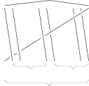
Figure 3: The closed braid $\ A_{i,j}\ (i,j\geq 0)$

Note that $A_{m}=A_{m-1,0}$ and $\overline{A}_{m}=A_{0,m-1}$.

We define the element $X_{m}$ in the skein $\mathcal{C}$, shown in figure 4, as the sum of $m$ closed $m$-braids,

$$X_{m}=\sum_{j=0}^{m-1}A_{m-1-j,j}.$$

$+$ at 320 90 $+\ \ \cdots\ \ +$ at 766 90

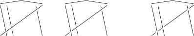
Figure 4: The element $X_{m}$

The elements $\overline{A}_{m}$ and $X_{m}$ are readily related to the elements $A_{m}$ by two formal power series formulae.

Write

$$A(t)=1+z\sum_{i=1}^{\infty}A_{i}t^{i}$$

and its mirror image

$$\overline{A(t)}=1-z\sum_{i=1}^{\infty}\overline{A}_{i}t^{i}.$$

Theorem 1.

$$A(t)\overline{A(t)}=1.$$

Theorem 2.

$$z\sum_{m=1}^{\infty}\frac{X_{m}}{m}t^{m}=\ln(A(t)).$$

These two theorems are consequences of a simple skein-theoretic lemma, originally used by Aiston in [1]. We set $A_{0}=\frac{1}{z}$ and $\overline{A}_{0}=-\frac{1}{z}$ to simplify the notation in the following statements.

Lemma 3.

For $i\geq 1$ we have $A_{i,j}=zA_{i}\overline{A}_{j+1}+A_{i-1,j+1}$.

Proof. Use the quadratic relation in the skein at the marked crossing to get

$j$ strings at 210 -25 $i$ strings at 500 -25 $A_{i,j}\quad=\quad\raisebox{-0.5pt}{\includegraphics[scale={.150}]{AijMarcado}}\quad=\quad zA_{i}\overline{A}_{j+1}+A_{i-1,j+1}.$

 

Lemma 4.

For $m\geq 1$ we have $\overline{A}_{m}=-z\sum_{k=1}^{m}A_{k}\overline{A}_{m-k}$.

Proof. Repeated use of lemma 3 gives

$$A_{m} = A_{m-1,0}$$

$$= zA_{m-1}\overline{A}_{1}+A_{m-2,1}$$

$$= zA_{m-1}\overline{A}_{1}+zA_{m-2}\overline{A}_{2}+A_{m-3,2}$$

$$\vdots$$

$$= zA_{m-1}\overline{A}_{1}+zA_{m-2}\overline{A}_{2}+\dots+zA_{1}\overline{A}_{m-1}+A_{0,m-1}.\$$

The last equation can be written

$$A_{m}=z\sum_{k=1}^{m-1}A_{m-k}\overline{A}_{k}+\overline{A}_{m}=z\sum_{k=1}^{m}\overline{A}_{k}A_{m-k}.$$

Now apply the mirror map.  

of theorem 1. The coefficient of $t^{m}$ in $A(t)\overline{A(t)}$ is

$$-z\overline{A}_{m}-z^{2}A_{1}\overline{A}_{m-1}-z^{2}A_{2}\overline{A}_{m-2}-\ldots-z^{2}A_{m-1}\overline{A}_{1}+zA_{m}$$

$$= z\left(A_{m}-\overline{A}_{m}-z\sum_{k=1}^{m-1}A_{k}\overline{A}_{m-k}\right).$$

This is $0$ for $m\geq 1$ by lemma 4, while the constant term is $1$.  

Lemma 5.

For $m\geq 1$ we have $X_{m}=-z\displaystyle\sum_{j=1}^{m}jA_{j}\overline{A}_{m-j}.$

Proof. Sum all the equations except the first in the proof of lemma 4 to get

$$(m-1)A_{m}=z((m-1)A_{m-1}\overline{A}_{1}+(m-2)A_{m-2}\overline{A}_{2}+...+A_{1}\overline{A}_{m-1})+\sum_{j=1}^{m-1}A_{m-1-j,j}.$$

Since $A_{m}=A_{m-1,0}$ it follows that

$$mA_{m}=z\sum_{j=1}^{m-1}jA_{j}\overline{A}_{m-j}+X_{m}.$$

 

of theorem 2. Since the constant terms in the two series are equal, it is enough to show that their derivatives are equal.

Now

$$\frac{d}{dt}\left(z\sum\frac{X_{m}}{m}t^{m}\right)=z\sum X_{m}t^{m-1}$$

and

$$\frac{d}{dt}\left(\ln(A(t))\right)=\frac{A^{\prime}(t)}{A(t)}=A^{\prime}(t)\overline{A(t)}$$

by theorem 1. The coefficient of $t^{m-1}$ in $A^{\prime}(t)\overline{A(t)}$ is

$$-z^{2}\displaystyle\sum_{j=1}^{m}jA_{j}\overline{A}_{m-j}=zX_{m}$$

by lemma 5, for all $m\geq 1$, and so the two series are equal.  

We shall use the power series relations to give expressions for $\overline{A}_{m}$ and $X_{m}$ in terms of the Turaev basis $\{A_{\lambda}\}_{\lambda\vdash m}$ for $\mathcal{C}_{m}$. The first of these depends on the general expression for the coefficients $\{d_{m}\}$ of the inverse, $1+\sum d_{m}t^{m}$, of a formal power series $1+\sum c_{n}t^{n}$, in terms of monomials in the coefficients $\{c_{n}\}$, while the second, which can be deduced quickly from the first, gives the coefficients of the logarithm of a formal power series. Both of these results can be found by applying the technique given in [10] (example 11, page 30) for finding the coefficients of the resulting power series when one power series is substituted in another.

When discussing monomials in the coefficients $\{c_{n}\}$ it is helpful to distinguish between ordered monomials, $c_{r_{1}}c_{r_{2}}\ldots c_{r_{l}}$, and the corresponding standard monomial $c_{\lambda_{1}}c_{\lambda_{2}}\ldots c_{\lambda_{l}}$, where the sequence $(r_{1},r_{2},\dots,r_{l})$ is rearranged into descending order $(\lambda_{1},\lambda_{2},\dots,\lambda_{l})$. The standard monomial can then be described as $c_{\lambda}$ where $\lambda$ is the partition of $m=\sum\lambda_{i}$ having $l$ parts $\lambda_{1}\geq\lambda_{2}\geq\dots\geq\lambda_{l}>0$. We write $k_{\lambda}$ for the number of ordered monomials with standard monomial $c_{\lambda}$, or equally the number of rearrangements of the sequence $(\lambda_{1},\lambda_{2},\dots,\lambda_{l})$.

The coefficient $d_{m}$ of $t^{m}$ in the inverse series is the sum over partitions $\lambda\vdash m$ of $(-1)^{l}k_{\lambda}c_{\lambda}$.

Theorem 6.

For $m\geq 1$ we have that

$$\overline{A}_{m}=\sum_{\lambda\vdash m}k_{\lambda}(-z)^{l-1}A_{\lambda}.$$

Proof. This follows at once from theorem 1 and the formula for the inverse series.  

There is a simple combinatorial formula for $k_{\lambda}$ as a multinomial coefficient, in terms of the multiplicities of the parts of $\lambda$. If $\lambda$ has $r$ distinct parts repeated $m_{1},\ldots,m_{r}$ times respectively, making a total of $l=m_{1}+\cdots+m_{r}$ parts altogether, there are ${l\choose{m_{1},\ldots,m_{r}}}=\displaystyle\frac{l!}{m_{1}!\cdots m_{r}!}=k_{\lambda}$ possible rearrangements.

Example.  The partition $\lambda=(4,4,4,2,2,1,1,1)$ with length $l=8$ has three distinct parts with multiplicities $m_{1}=3,m_{2}=2$ and $m_{3}=3$, hence $k_{\lambda}=\frac{8!}{3!\ 2!\ 3!}=560$. It follows from theorem 6 that the coefficient of $A_{4}^{3}A_{2}^{2}A_{1}^{3}$ in $\overline{A}_{19}$ is $-560z^{7}$.

Theorem 7.

$X_{m}$ is given in terms of the monomials $\{A_{\lambda}\}_{\lambda\vdash m}$ by the formula

$$X_{m}=m\sum_{\lambda\vdash m}\frac{k_{\lambda}}{l}(-z)^{l-1}A_{\lambda}.$$

Proof. Differentiate $\ln(A(t))$ with respect to $z$, treating each $A_{i}$ as constant.

By theorem 1

$$\frac{d}{dz}\left(\ln(A(t))\right) = \frac{d}{dz}(A(t))/A(t)=\frac{d}{dz}(A(t))\times\overline{A(t)}$$

$$= \frac{A(t)-1}{z}\times\overline{A(t)}=\frac{1-\overline{A(t)}}{z}$$

$$= \sum_{m=1}^{\infty}\overline{A}_{m}t^{m}.$$

By theorems 2 and 6, we have

$$\frac{d}{dz}(zX_{m}/m)=\overline{A}_{m}=\sum_{\lambda\vdash m}k_{\lambda}(-z)^{l-1}A_{\lambda}.$$

Integrating the right hand side gives

$$\frac{zX_{m}}{m}=\sum_{\lambda\vdash m}k_{\lambda}(-1)^{l-1}\frac{z^{l}}{l}A_{\lambda},$$

and the theorem follows.  

Example.  For the partition $\lambda=(3,3,1,1,1)$ we have $m=9,l=5,m_{1}=2$ and $m_{2}=3$. Then $k_{\lambda}=\frac{5!}{2!\ 3!}=10$ and the coefficient of $A_{3}^{2}A_{1}^{3}$ in $X_{9}$ is

$$m\frac{k_{\lambda}}{l}(-z)^{l-1}=9\frac{10}{5}(-z)^{5-1}=18z^{4}.$$

4 Symmetric functions

The element $h_{m}\in{\cal C}_{m}$, which is taken to represent the complete symmetric function of degree $m$, is the closure of the element $\frac{1}{\alpha_{m}}a_{m}\in H_{m}$ where $a_{m}=\sum_{\pi\in S_{m}}s^{l(\pi)}\omega_{\pi}$ is one of the two basic quasi-idempotent elements of $H_{m}$. Here $\omega_{\pi}$ is the positive permutation braid associated to the permutation $\pi\in S_{m}$ with length $l(\pi)$ and $\alpha_{m}$ is given by the equation $a_{m}a_{m}=\alpha_{m}a_{m}$ [9, 2, 11]. Using the other quasi-idempotent $b_{m}=\sum_{\pi\in S_{m}}(-s)^{-l(\pi)}\omega_{\pi}$ in a similar way determines the element $e_{m}$ which represents the elementary symmetric function. These elements are related by the power series equation $H(t)E(-t)=1$, where $H(t)=1+\sum h_{n}t^{n}$ and $E(t)=1+\sum e_{n}t^{n}$. The involution on the skein $\mathcal{C}$ induced by sending each diagram to itself and altering the coefficients by fixing $v$ and interchanging $s$ with $-s^{-1}$ will interchange $h_{m}$ and $e_{m}$.

The subalgebra $\mathcal{C}_{+}$ of $\mathcal{C}$ is generated as an algebra by $\{h_{n}\}$, and the monomials $h_{\lambda}$ of weight $m$, where $\lambda\vdash m$, form a basis for $\mathcal{C}_{m}$, allowing $\mathcal{C}_{+}$ to be interpreted as the ring of symmetric functions in variables $x_{1},\ldots,x_{N},\ldots$ with coefficients in $\Lambda$. In this interpretation $\mathcal{C}_{m}$ consists of the homogeneous functions of degree $m$.

The power sums $P_{m}=\sum x_{i}^{m}$ are symmetric functions which can be written in terms of the complete symmetric functions by Newton’s power sum relation $\ln H(t)=\sum_{m}\frac{P_{m}}{m}t^{m}$. This equation defines $P_{m}$ as an element of the skein $\mathcal{C}_{m}$. The element $P_{m}$ is used in [11] for describing the $m$th power sum of the Murphy operators in $H_{n}$, independently of $n$. It is shown in [12] that the more geometric element $X_{m}$ in figure 4 is a scalar multiple of $P_{m}$, given explicitly as $X_{m}=[m]P_{m}$, where $[m]$ is the quantum integer $\displaystyle\frac{s^{m}-s^{-m}}{s-s^{-1}}$.

Theorem 7 gives the immediate expression

$$P_{m}=\frac{m}{[m]}\sum_{\lambda\vdash m}\frac{k_{\lambda}}{l}(-z)^{l-1}A_{\lambda}$$ (1)

for $P_{m}$ in Turaev’s basis.

The complete symmetric functions $\{h_{n}\}$ themselves are shown in theorem 3.6 of [11] to be related to Turaev’s closed braids $\{A_{m}\}$ by the equation

$$A(t)=\frac{H(st)}{H(s^{-1}t)}.$$ (2)

We now derive an expression for $h_{m}$ in terms of Turaev’s basis. We had hoped for a more illuminating way to display the coefficient of $A_{\lambda}$ in terms of the partition $\lambda\vdash m$, but we do have an explicit rational function in $\Lambda$ whose numerator may be able to be reorganised better in some given cases.

4.1 The complete symmetric functions $h_{m}$

Equation (2) can be written in the form $H(s^{-1}t)A(t)-H(st)=0$. Equivalently

$$\left(\sum_{n=0}^{\infty}s^{-n}h_{n}t^{n}\right)\left(1+z\sum_{m=1}^{\infty}A_{m}t^{m}\right)-\sum_{n=0}^{\infty}s^{n}h_{n}t^{n}=0.$$

Considering the coefficient of $t^{m}$ we obtain the equation

$$s^{-m}h_{m}+z\sum_{j=0}^{m-1}s^{-j}h_{j}A_{m-j}-s^{m}h_{m}=0,$$

hence

$$[m]h_{m}=\sum_{j=0}^{m-1}s^{-j}h_{j}A_{m-j}.$$

For a partition $\lambda=(\lambda_{1},\dots,\lambda_{l})$ of $m$, we will write $l_{i}$ for the multiplicity of the part $\lambda_{i}$ in $\lambda$. We will also write $\lambda-\lambda_{i}$ for the partition $(\dots,\lambda_{i-1},\lambda_{i+1},\dots)\vdash m-\lambda_{i}$ with length $l-1$.

Theorem 8.

The complete symmetric functions can be written as

$$h_{m}=\sum_{\lambda\vdash m}\theta_{\lambda}\ A_{\lambda},$$

where $\theta_{\lambda}$ is given recursively by the formula

$$\theta_{\lambda}=\frac{1}{s^{m}[m]}\ \sum_{i=1}^{l}\frac{s^{\lambda_{i}}}{l_{i}}\ \theta_{\lambda-\lambda_{i}}$$

and $\theta_{\emptyset}=1$, where $\emptyset$ denotes the empty partition.

Proof. We prove the theorem by induction on $m$. For $m=1$ we have that $\lambda=(1)$ is the only partition of $1$ and $\theta_{(1)}=1$, hence the formula just says that $h_{1}=A_{1}$. Assume the theorem for $1,\dots,m-1$. Then

$$[m]h_{m} = \sum_{j=0}^{m-1}s^{-j}h_{j}A_{m-j}$$

$$= \sum_{j=0}^{m-1}s^{-j}A_{m-j}\left(\sum_{\mu\vdash j}\theta_{\mu}\ A_{\mu_{1}}\cdots A_{\mu_{l}}\right)\ \ \ \ \mbox{(by induction)}$$

$$= \sum_{\lambda\vdash m}\left(\sum_{i=1}^{l}\frac{s^{-(m-\lambda_{i})}}{l_{i}}\ \theta_{\lambda-\lambda_{i}}\right)A_{\lambda_{1}}\cdots A_{\lambda_{l}},$$

and $\theta_{\lambda}$ is obviously the expression in brackets divided by $[m]$.  

Remark.  The coefficient of $A_{1}^{m}$ in $h_{m}$ is $\theta_{(1,\stackrel{{\scriptstyle m}}{{\dots}},1)}=\frac{1}{\alpha_{m}}$, where $\alpha_{m}=s^{\frac{m(m-1)}{2}}[m]!$ satisfies the equation $a_{m}^{2}=\alpha_{m}a_{m}$. Also the coefficient of $A_{m}$ in $h_{m}$ is $\theta_{(m)}=\frac{1}{[m]}$.

We now provide a non-recursive formula for the coefficients $\{\theta_{\lambda}\}$ of theorem 8. First, we introduce some notation: if $\mu=(\mu_{1},\dots,\mu_{l})$ is a (not necessarily decreasing) finite sequence of integers $\mu_{j}>0$, we define the coefficient

$$c_{\mu}=\prod_{i=1}^{l}\frac{1}{[\mu_{1}+\dots+\mu_{i}]s^{\mu_{1}+\dots+\mu_{i}}}.$$

If $\lambda=(\lambda_{1},\dots,\lambda_{l})$ is a partition with length $l$ and $\alpha\in S_{l}$, the set of permutations of $\{1,2,\dots,l\}$, we will write $\lambda_{\alpha}$ for the finite sequence $\lambda_{\alpha}=(\lambda_{\alpha(1)},\dots,\lambda_{\alpha(l)})$.

Lemma 9.

For a partition $\lambda$ of $m$ with length $l$ the coefficient $\theta_{\lambda}$ can be written as

$$\theta_{\lambda}=\frac{k_{\lambda}}{l!}s^{m}\sum_{\alpha\in S_{l}}c_{\lambda_{\alpha}}.$$

Proof. By induction on the length $l$ of the partition $\lambda$. If $l=1$ we have $\theta_{\lambda}=\theta_{(m)}=\frac{1}{[m]}$, and the right hand side is

$$\frac{k_{(m)}}{1!}s^{m}\frac{1}{[m]s^{m}}=\frac{1}{[m]}.$$

Assume now the formula for $1,\dots,l-1$ and consider a partition $\lambda=(\lambda_{1},\dots,\lambda_{l})\vdash m$ with length $l$. By definition

$$\theta_{\lambda}=\frac{1}{s^{m}[m]}\sum_{i=1}^{l}\frac{s^{\lambda_{i}}}{l_{i}}\theta_{\lambda-\lambda_{i}}$$

and by induction (the partitions $\lambda-\lambda_{i}$ have length $l-1$), we have that

$$\theta_{\lambda}=\frac{1}{s^{m}[m]}\sum_{i=1}^{l}\left(\frac{s^{\lambda_{i}}}{l_{i}}\frac{k_{\lambda-\lambda_{i}}}{(l-1)!}s^{m-\lambda_{i}}\sum_{\beta\in S_{l-1}}c_{(\lambda-\lambda_{i})_{\beta}}\right).$$

Since $k_{\lambda-\lambda_{i}}=k_{\lambda}\frac{l_{i}}{l}$, we deduce that

$$\theta_{\lambda}=\frac{k_{\lambda}}{l![m]}\sum_{i=1}^{l}\sum_{\beta\in S_{l-1}}c_{(\lambda-\lambda_{i})_{\beta}}.$$

For every $1\leq i\leq l$ and permutation $\beta\in S_{l-1}$ we define the permutation $\alpha\in S_{l}$ as the composite permutation $\alpha=\beta\ (l,i,i+1,\dots,l-1)$ which maps $l$ to $i$, establishing a bijection between $\{1,\dots,l\}\times S_{l-1}$ and $S_{l}$. It turns out that $\lambda_{i}$ is the last part of $\lambda_{\alpha}$, and $\lambda_{\alpha}-(\lambda_{\alpha})_{l}=(\lambda-\lambda_{i})_{\beta}$. It follows that $[m]s^{m}c_{\lambda_{\alpha}}=c_{(\lambda-\lambda_{i})_{\beta}}$, hence

$$\theta_{\lambda}=\frac{k_{\lambda}}{l![m]}\sum_{\alpha\in S_{l}}[m]s^{m}c_{\lambda_{\alpha}}=\frac{k_{\lambda}}{l!}s^{m}\sum_{\alpha\in S_{l}}c_{\lambda_{\alpha}}.$$

 

Example.  We have

$$\begin{array}[]{l}h_{1}=A_{1},\\ h_{2}=\frac{s}{s^{2}+1}A_{2}+\frac{1}{s^{2}+1}A_{1}^{2},\\ h_{3}=\frac{s^{2}}{s^{4}+s^{2}+1}A_{3}+\frac{s(s^{2}+2)}{(s^{4}+s^{2}+1)(s^{2}+1)}A_{2}A_{1}+\frac{1}{(s^{4}+s^{2}+1)(s^{2}+1)}A_{1}^{3},\ {\rm etc.}\end{array}$$

For example, for $\lambda=(2,1)$, we have $k_{\lambda}=2$, $l=2$, $m=3$, $c_{(2,1)}=\frac{1}{[2][3]s^{5}}$ and $c_{(1,2)}=\frac{1}{[3]s^{4}}$, giving the coefficient of $A_{2}A_{1}$ in $h_{3}$ as $\theta_{(2,1)}=\frac{s(s^{2}+2)}{(s^{4}+s^{2}+1)(s^{2}+1)}$.

In general each coefficient in $h_{m}$ is a rational function with denominator $[m]!$. As a further example, the coefficient $\theta_{(3,3,2)}$ of $A_{3}^{2}A_{2}$ in $h_{8}$ is

$$\ \frac{s^{8}}{2}(2c_{(3,3,2)}+2c_{(3,2,3)}+2c_{(2,3,3)})=s^{8}\left(\frac{1}{s^{17}[3][6][8]}+\frac{1}{s^{16}[3][5][8]}+\frac{1}{s^{15}[2][5][8]}\right).$$

Corollary 10.

We have a similar formula for the elementary symmetric functions,

$$e_{m}=\sum_{\lambda\vdash m}\tau_{\lambda}\ A_{\lambda},$$

where, for each partition $\lambda\vdash m$ with length $l$, the coefficient $\tau_{\lambda}$ is

$$\tau_{\lambda}=(-1)^{m+l}\frac{k_{\lambda}}{l!}s^{-m}\sum_{\alpha\in S_{l}}\prod_{i=1}^{l}\frac{s^{\lambda_{\alpha(1)}+\dots+\lambda_{\alpha(i)}}}{[\lambda_{\alpha(1)}+\dots+\lambda_{\alpha(i)}]}.$$

Proof. The element $e_{m}$ can be obtained from $h_{m}$ with the substitution $s=-s^{-1}$. After this substitution, $[k]s^{k}$ becomes $-\frac{[k]}{s^{k}}$.  

5 Schur functions and hook partitions

The meridian maps, introduced explicitly in [11], are linear maps $\varphi,\overline{\varphi}:\mathcal{C}\to\mathcal{C}$, induced by including an oriented meridian around any diagram $X$ in the annulus as shown in figure 5.

$X$ at 22 262 $\varphi(X)\ =\ \raisebox{-0.5pt}{\includegraphics[scale={.20}]{meridianmap}}\quad\quad\overline{\varphi}(X)\ =\ {\labellist\small\pinlabel{$X$}at22262\endlabellist}\raisebox{-0.5pt}{\includegraphics[scale={.20}]{meridianmapRev}}$

Figure 5: The meridian maps

It is shown in [5] that the eigenvectors of $\varphi$ have no repeated eigenvalues, and that there is a basis $Q_{\lambda,\mu}$ of $\mathcal{C}$ consisting of these eigenvectors, where $\lambda$ and $\mu$ run through all pairs of partitions. The subspace $\mathcal{C}_{m}$ has a basis $Q_{\lambda,\phi}=Q_{\lambda}$, where $\lambda$ runs through partitions of $m$.

This basis has been identified by Lukac with the basis formed by the closures $Q_{\lambda}$ of Aiston’s idempotent elements $e_{\lambda}$ in the Hecke algebra $H_{m}$. Lukac has shown also that they represent the Schur functions $s_{\lambda}$ in the interpretation as symmetric functions. Thus they can be expressed as determinants of the elements $h_{m}$ by the Jacobi-Trudi formula; precisely, $Q_{\lambda}={\rm det}(h_{\lambda_{i}+j-i})_{1\leq i,j\leq l}$ if $\lambda=(\lambda_{1},\dots,\lambda_{l})$ ([9, 5]). Since $\overline{h}_{i}=h_{i}$ ([11], lemma 3.7), the elements $Q_{\lambda}$ are not affected by the mirror map.

As extreme cases we have $Q_{\lambda}=h_{m}$ when $\lambda=(m)$ is a row partition, and $Q_{\lambda}=e_{m}$ when $\lambda=(1,\stackrel{{\scriptstyle m}}{{\dots}},1)$ is a column partition. In Frobenius notation, $(a|b)$ denotes the hook partition of $m=a+b+1$ with an arm of length $a$ and a leg of length $b$, as shown in figure 6.

$a$ at 91 105 $b$ at 6 38

Figure 6: The hook $(a|b)$

The hook partitions of $m$ include the single row $(m-1|0)$ and the single column $(0|m-1)$. The power sums can be written, by the Frobenius character formula, as $P_{m}=\sum_{a+b=m-1}(-1)^{b}Q_{(a|b)}$ ([4], 4.10, 4.16). In particular, $P_{m}$ is not affected by the mirror map. Since $\overline{[m]}=[m]$, we have also that $\overline{X}_{m}=X_{m}$.

The Pieri formula for products of Schur functions ([10], page 73) shows that $h_{i}e_{j}$ is the sum of the Schur functions of two hook partitions $(i-1|j)$ and $(i|j-1)$. We can write explicitly $h_{i}e_{j}=Q_{(i-1|j)}+Q_{(i|j-1)}$ for all $i,j\geq 0$, by setting $Q_{(i|j)}=0$ when $i<0$ or $j<0$. We can use equation (2) to write $A_{m}$ in the basis $\{Q_{\lambda}\}_{\lambda\vdash m}$, where the only partitions $\lambda$ required are hooks of length $m$.

Theorem 11.

$$A_{m}=\sum_{a+b=m-1}(-1)^{b}s^{a-b}Q_{(a|b)}.$$

Proof. By equation (2) we have

$$A(t)=\frac{H(st)}{H(s^{-1}t)}={H(st)}{E(-s^{-1}t)}.$$

Comparing the coefficients of $t^{m}$, taking $h_{0}=e_{0}=1$, gives

$$zA_{m} = \sum_{i+j=m}s^{i}h_{i}(-1)^{j}s^{-j}e_{j}=\sum_{i+j=m}(-1)^{j}s^{i-j}h_{i}e_{j}$$

$$= \sum_{i+j=m}(-1)^{j}s^{i-j}\left(Q_{(i-1|j)}+Q_{(i|j-1)}\right).$$

We can rewrite the sum as

$$\sum_{a+b=m-1}(-1)^{b}s^{a+1-b}Q_{(a|b)}+\sum_{a+b=m-1}(-1)^{b+1}s^{a-b-1}Q_{(a|b)}$$

$$= (s-s^{-1})\sum_{a+b=m-1}(-1)^{b}s^{a-b}Q_{(a|b)},$$

giving the result, since $z=s-s^{-1}$.  

The formula obtained in theorem 11 resembles the formula obtained by Rosso and Jones in [14], theorem 8. They remark there that the only partitions which occur when calculating the Homfly polynomial of the torus knots are hooks. We show later how to deduce theorem 11 from theorem 13, which makes use of quantum invariants and [14] in its proof.

We can now give a simpler diagrammatic representation of $P_{m}$ using theorem 11 and the meridian map $\varphi$. For $Q\in\mathcal{C}$ set $\Delta_{\varphi}(Q)=\varphi(Q)-\delta Q\in\mathcal{C}$ and $\Delta_{\overline{\varphi}}(Q)=\overline{\varphi}(Q)-\delta Q\in\mathcal{C}$.

Theorem 12.

We have

$$(s-s^{-1})X_{m}=v\Delta_{\varphi}(\overline{A}_{m})=-v^{-1}\Delta_{\overline{\varphi}}(A_{m}),$$

hence

$$\{m\}P_{m}=v\Delta_{\varphi}(\overline{A}_{m})=-v^{-1}\Delta_{\overline{\varphi}}(A_{m}).$$

Proof. Applying the mirror map to the equation of theorem 11 we get

$$\overline{A}_{m}=\sum_{(a|b)\vdash m}(-1)^{b}s^{b-a}Q_{(a|b)}.$$

It follows that

$$\Delta_{\varphi}(\overline{A}_{m})=\sum_{(a|b)\vdash m}(-1)^{b}s^{b-a}\Delta_{\varphi}(Q_{(a|b)}).$$

In general,

$$\Delta_{\varphi}(Q_{\lambda})=v^{-1}(s-s^{-1})\sum_{x\in\lambda}s^{2c(x)}Q_{\lambda}$$ (3)

where the sum runs over cells $x\in\lambda$ and $c(x)=j-i$ is the content of the cell $x$ in position $(i,j)$, which can be deduced from [5], theorem 3.4.

For $\lambda=(a|b)\vdash m$ we have $\displaystyle\sum_{x\in\lambda}s^{2c(x)}=\frac{s^{m}-s^{-m}}{s-s^{-1}}s^{a-b}$, hence in particular

$$\Delta_{\varphi}(Q_{(a|b)})=v^{-1}(s^{m}-s^{-m})s^{a-b}Q_{(a|b)}.$$

Then

$$v\Delta_{\varphi}(\overline{A}_{m}) = (s^{m}-s^{-m})\sum_{(a|b)\vdash m}(-1)^{b}Q_{(a|b)}$$

$$= (s^{m}-s^{-m})P_{m}=\{m\}P_{m}$$

$$= (s-s^{-1})X_{m}.$$

Applying the mirror map gives the other representation.  

Hence we have an even simpler diagrammatic representative for $P_{m}$ in $\mathcal{C}$ in terms of just two closed tangles, as seen in figure 7.

$-$ at 346 217

$v^{-1}\{m\}P_{m}=$

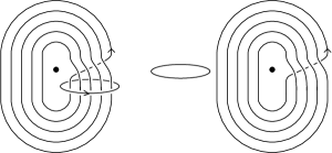
Figure 7: A representation of $P_{m}$ by two tangles

6 Satellite and quantum $sl(N)$ invariants

One of the most useful features of the skein $\mathcal{C}$ is its role in parametrising Homfly satellite invariants of a framed knot $K$.

6.1 Satellites

A satellite of $K$ is determined by choosing a diagram $Q$ in the standard annulus, and then drawing $Q$ on the annular neighbourhood of $K$ determined by the framing, to give the satellite knot $K*Q$. We refer to this construction as decorating $K$ with the pattern $Q$ (see figure 8).

$Q=$ at -60 195 $K=$ at 430 195 $K*Q=$ at 1060 195

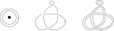
Figure 8: Satellite construction

The Homfly polynomial $P(K*Q)$ of the satellite depends on $Q$ only as an element of the skein $\mathcal{C}$ of the annulus, hence we can extend the definition of $K*Q$ to cover a general element $Q\in\mathcal{C}$ if we are only concerned with its Homfly polynomial. We regard $\mathcal{C}$ as the natural parameter space for these invariants of $K$, known collectively as the Homfly satellite invariants of $K$. We use the notation $P(K;Q)$ in place of $P(K*Q)$ when we want to emphasise the dependence on $K$. When $Q$ is restricted to lie in $\mathcal{C}_{m}$ the invariants are called the $m$-string satellite invariants, and can be realised as linear combination of a finite number of satellite invariants. For example any closed $m$-braid $Q=\hat{\beta}$ in the annulus determines an element of $\mathcal{C}_{m}$ which can be written as $Q=\sum_{\lambda\vdash m}c_{\lambda}Q_{\lambda}$ in terms of the basis $\{Q_{\lambda}\}_{\lambda\vdash m}$, with coefficients $c_{\lambda}\in\Lambda$. The Homfly polynomial of the satellite $K*Q$ is then $P(K*Q)=\sum c_{\lambda}P(K*Q_{\lambda})$.

The same overall collection of invariants of $K$ can be constructed from the quantum invariants arising from the quantum groups $sl(N)_{q}$.

Here is a brief summary of the interrelations. A more extensive account can be found in the thesis of Lukac ([8]), including details of variant Homfly skeins with a framing correction factor, $x$. These are isomorphic to the skeins used here but the parameter allows a careful adjustment of the quadratic skein relation to agree directly with the natural relation arising from use of the quantum groups $sl(N)_{q}$.

6.2 Quantum invariants

Quantum groups give rise to 1-parameter invariants $J(K;W)$ of an oriented framed knot $K$ depending on a choice of finite dimensional module $W$ over the quantum group, following constructions of Turaev and others ([15, 17, 2]). This choice is referred to as colouring $K$ by $W$, and can be extended for a link allowing a choice of colour for each component.

Fix a natural number $N$. When we colour $K$ by a finite dimensional module $W$ over the quantum group $sl(N)_{q}$, its invariant $J(K;W)$ depends on one variable $s$. The invariant $J$ is linear under the direct sum of modules and all the modules over $sl(N)_{q}$ are semi-simple, so we can restrict our attention to the irreducible modules $V_{\lambda}^{(N)}$. For $sl(N)_{q}$ these are indexed by partitions $\lambda$ with at most $N$ parts, without distinguishing two partitions which differ in some initial columns with $N$ cells.

Remark.  (Comparison theorem)

1. The $sl(N)_{q}$ invariant for the irreducible module $V_{\lambda}^{(N)}$ is the Homfly invariant for the knot decorated by $Q_{\lambda}$ with $v=s^{-N}$, suitably normalised as in [8]. Explicitly,

   $$P(K*Q_{\lambda})|_{v=s^{-N}}=x^{k|\lambda|^{2}}J(K;V_{\lambda}^{(N)})$$

   where $k$ is the writhe of $K$, $x=s^{1/N}$ and $|\lambda|=\sum\lambda_{i}$.

2. Each invariant $P(K*Q)|_{{v=s^{-N}}}$ is a linear combination $\sum c_{\alpha}J(K;W_{\alpha})$ of quantum invariants .

3. Each $J(K;W)$ is a linear combination $\sum d_{j}P(K*Q_{j})|_{{v=s^{-N}}}$ of Homfly invariants.

Remark.  The 2-variable invariant $P(K*Q)$ can be recovered from the specialisations $P(K*Q)|_{{v=s^{-N}}}$ for sufficiently many $N$.

Remark.  If the pattern $Q$ is a closed braid on $m$ strings then we only need use partitions $\lambda\vdash m$, since $\mathcal{C}_{m}$ is spanned by $\{Q_{\lambda}\}_{\lambda\vdash m}$. Conversely, to realise $J(K;V_{\lambda}^{(N)})$ with $\lambda\vdash m$ we can use closed $m$-braid patterns.

6.3 Basic constructions

A quantum group $\cal G$ is an algebra over a formal power series ring ${\bf Q}[[h]]$, typically a deformed version of a classical Lie algebra. We write $q=e^{h},s=e^{h/2}$ when working in $sl(N)_{q}$. A finite dimensional module over $\cal G$ is a linear space on which $\cal G$ acts.

Crucially, $\cal G$ has a coproduct $\Delta$ which ensures that the tensor product ${V\otimes W}$ of two modules is also a module. It also has a universal $R$-matrix (in a completion of ${\cal G}\otimes{\cal G}$) which determines a well-behaved module isomorphism

$$R_{VW}:V\otimes W\to W\otimes V.$$

This has a diagrammatic view indicating its use in converting coloured tangles to module homomorphisms:

$W\ \otimes\ V$ at 165 156 $V\ \otimes\ W$ at 165 12 $R_{VW}$ at -50 84

A braid $\beta$ on $m$ strings with permutation $\pi\in S_{m}$ and a colouring of the strings by modules $V_{1},\ldots,V_{m}$ leads to a module homomorphism

$$J_{\beta}:V_{1}\otimes\cdots\otimes V_{m}\to V_{\pi(1)}\otimes\cdots\otimes V_{\pi(m)}$$

using $R_{V_{i},V_{j}}^{\pm 1}$ at each elementary braid crossing. The homomorphism $J_{\beta}$ depends only on the braid $\beta$ itself, not its decomposition into crossings, by the Yang-Baxter relation for the universal $R$-matrix.

When $V_{i}=V$ for all $i$ we get a module homomorphism $J_{\beta}:W\to W$, where $W=V^{\otimes m}$. Now any module $W$ decomposes as a direct sum $\bigoplus{(W_{\mu}\otimes V_{\mu}^{(N)})}$, where $W_{\mu}\subset W$ is a linear subspace consisting of the highest weight vectors of type $\mu$ associated to the module $V_{\mu}^{(N)}$. Highest weight subspaces of each type are preserved by module homomorphisms, and so $J_{\beta}$ determines (and is determined by) the restrictions $J_{\beta}(\mu):W_{\mu}\to W_{\mu}$ for each $\mu$, where $\mu$ runs over partitions with at most $N$ parts.

If a knot (or one component of a link) $K$ is decorated by a pattern $T$ which is the closure of an $m$-braid $\beta$, then its quantum invariant $J(K*T;V)$ can be found from the endomorphism $J_{\beta}$ of $W=V^{\otimes m}$ in terms of the quantum invariants of $K$ and the restriction maps $J_{\beta}(\mu):W_{\mu}\to W_{\mu}$ by the formula

$$J(K*T;V)=\sum c_{\mu}J(K;V_{\mu}^{(N)})$$ (4)

with $c_{\mu}=\mbox{tr}\,J_{\beta}(\mu)$. This formula follows from lemma II.4.4 in Turaev’s book [16]. We set $c_{\mu}=0$ when $W$ has no highest weight vectors of type $\mu$.

6.4 Invariants of satellites

The quantum invariant $J(K*T;V)$, where $V=\bigoplus V_{\lambda}^{(N)}$ is decomposed into irreducible modules, is the sum $\sum J(K*T;V_{\lambda}^{(N)})$. This is given by the sum of Homfly satellite invariants $\sum P(K*T;Q_{\lambda})$, with $v=s^{-N}$, after adjustment by the framing correction parameter $x$.

To discuss these further we note that the satellite $(K*T)*Q$ of $K*T$ when decorated with a pattern $Q$ can also be viewed as $K*(T*Q)$, namely the satellite of $K$ when decorated by the pattern $T*Q$ in the annulus. For a general element $Q=\sum c_{i}Q_{i}$ in $\mathcal{C}$, written as a linear combination of diagrams $Q_{i}$, we can define $T*Q$ as an element of $\mathcal{C}$ by $T*Q=\sum c_{i}T*Q_{i}$. This leads to the equation

$$P(K*T;Q)=P(K;T*Q),$$

where $T$ is a diagram in the annulus and $Q\in\mathcal{C}$.

Hence we can find the Homfly polynomial $P(K*T;Q_{\lambda})$ as the satellite invariant $P(K;T*Q_{\lambda})$, which in turn can be found by writing $T*Q_{\lambda}$ in terms of the basis elements of the skein $\mathcal{C}$. Where $T$ is a closed $m$-braid and $\lambda\vdash d$, this element lies in $\mathcal{C}_{md}$ and we have

$$T*Q_{\lambda}=\sum_{\mu\vdash md}a_{\mu}Q_{\mu}$$

for some $a_{\mu}\in\Lambda$, giving

$$P(K*T;Q_{\lambda})=\sum_{\mu\vdash md}a_{\mu}P(K;Q_{\mu}).$$

Remark.  The same is true if the diagram $T$ is the closure of an $m$-tangle with all strings oriented in the same direction, but we must use the full basis elements $Q_{\nu,\rho}$ when $T$ is the closure of a tangle with some reverse oriented strings.

7 Cables and plethysms

The work of Rosso and Jones on traces in quantum groups, [14], gives us a skein theoretic description of $T*Q$ in the annulus where $T=T_{m}^{n}$ is a cable diagram, and $Q$ is an element of $\mathcal{C}_{+}$.

By the cable diagram $T_{m}^{n}$ we mean the diagram in the annulus formed by closing the framed $m$-braid $(\beta_{m})^{n}$ shown in figure 9. With the blackboard framing, $T_{m}^{n}$ is the diagram of the $(m,n)$ torus link with framing given by its neighbourhood in the surface of the torus. When $n=1$ we have $T_{m}^{1}=v^{-1}A_{m}$ as an element of $\mathcal{C}$ because of the choice of framing.

$m$ at 134 -25

$\beta_{m}$ = 

Figure 9: $T_{m}^{n}$ is the closure of $(\beta_{m})^{n}$

If $m$ and $n$ have highest common factor $d$ we can regard $T_{m}^{n}$ as the $d$-fold parallel of a torus knot diagram, and reduce our calculations to the case where $m$ and $n$ are coprime. In this case the cable diagram $T_{m}^{n}$ induces a map $F_{m}^{n}:\mathcal{C}\to\mathcal{C}$ taking an element $Q\in\mathcal{C}$ to the satellite $T_{m}^{n}*Q$.

The framing change map is the map $\tau=F_{1}^{1}$, illustrated in figure 10 by its effect on the 2-parallel element $(A_{1})^{2}$.

Figure 10: The framing change map on a $2$-parallel

It is shown in [2], theorem 17, that $\tau(Q_{\lambda})=\tau_{\lambda}Q_{\lambda}$ where $\tau_{\lambda}=v^{k}s^{r}$ with $k=-|\lambda|$ and $\displaystyle r=2\sum_{x\in\lambda}c(x)$.

We define a fractional twist map $\tau^{\frac{n}{m}}:{\cal C_{+}}\to{\cal C_{+}}$ as the linear map defined on the basis $\{Q_{\lambda}\}$ by

$$\tau^{\frac{n}{m}}(Q_{\lambda})=(\tau_{\lambda})^{\frac{n}{m}}Q_{\lambda}.$$

Remark.  Since the basis vectors $Q_{\lambda,\mu}$ for $\mathcal{C}$ are also eigenvectors of the framing change map, [5], we could define $\tau^{\frac{n}{m}}$ on the whole of $\mathcal{C}$ in a similar way, using the fact that $Q_{\lambda,\mu}$ has eigenvalue $\tau_{\lambda,\mu}=v^{k}s^{r}$ with $k=|\mu|-|\lambda|$ and $\displaystyle r=2\sum_{x\in\lambda}c(x)-2\sum_{x\in\mu}c(x)$.

To give the formula for $F_{m}^{n}(Q)$ with $Q\in\mathcal{C}_{+}$ we shall use the interpretation of $\mathcal{C}_{+}$ as the ring of symmetric functions, and adopt the terminology of plethysms to describe the resulting elements of the skein.

7.1 Plethysm

Let $p(x_{1},\dots,x_{N})=M_{1}+\dots+M_{r}$ be a symmetric polynomial in $N$ variables, which can be written as a sum of $r$ monomials, each with coefficient $1$. These include the Schur functions and the power sums. Let $q(x_{1},\dots,x_{r})$ be a symmetric function in $r$ variables. The plethysm $q[p]$ is the symmetric function of $N$ variables

$$q[p]=q(M_{1},\dots,M_{r}).$$

Remark.  A more general definition covering all symmetric polynomials $p$, along with further properties of plethysms, can be found in [10], where the notation $q\circ p$ is used in place of $q[p]$. We adopt here the notation from [3].

We can write the symmetric polynomial $q[p]$ in the basis of Schur functions as the linear combination

$$q[p]=\sum_{\nu}b_{qp}^{\nu}s_{\nu}.$$

Determining the coefficients $b_{qp}^{\nu}$ is in general a non-trivial problem. If $p$ and $q$ are themselves Schur functions $s_{\lambda}$ and $s_{\mu}$ respectively, we write

$$s_{\mu}[s_{\lambda}]=\sum_{\nu}a_{\mu\lambda}^{\nu}s_{\nu}.$$

It is shown in [10] that $a_{\mu\lambda}^{\nu}$ is a non-negative integer in all cases. It is a feature of many such calculations with symmetric polynomials that the coefficients are independent of the number of variables, $N$, under the condition that we take $s_{\nu}=0$ when $\nu$ has more than $N$ parts.

Here are some properties of plethysms that we will use shortly:

1. $q[p]$ is linear in $q$: $(a_{1}q_{1}+a_{2}q_{2})[p]=a_{1}q_{1}[p]+a_{2}q_{2}[p]$, for any scalars $a_{1},a_{2}$.

2. In general $q[p]$ is not linear in $p$, but if $q=P_{m}$ is a power sum, then $q[A+B]=q[A]+q[B]$, where $A$ and $B$ are both sums of monomials. For if $A=A_{1}+\dots+A_{r}$ and $B=B_{1}+\dots+B_{s}$, then $P_{m}[A+B]=A_{1}^{m}+\dots+A_{r}^{m}+B_{1}^{m}+\dots+B_{s}^{m}=P_{m}[A]+P_{m}[B].$

3. $s_{\lambda}[P_{m}]=P_{m}[s_{\lambda}]$ for any partition $\lambda$.

4. $P_{d}[P_{m}]=P_{md}=P_{m}[P_{d}]$, since $P_{d}[P_{m}]=(x_{1}^{m})^{d}+\dots+(x_{r}^{m})^{d}=x_{1}^{md}+\dots+x_{r}^{md}=P_{md}$.

Let $Q$ be any element of $\mathcal{C}_{+}$, regarded as a symmetric function, and let $P\in\mathcal{C}_{+}$ represent a sum of monomials each with coefficient $+1$, for example $P=P_{m}$ or $P=Q_{\lambda}$. We adopt the notation $Q[P]\in\mathcal{C}_{+}$ for the element corresponding to the plethysm of the functions represented by $Q$ and $P$.

With this notation we can give a compact formula for the element $F_{m}^{n}(Q)=T_{m}^{n}*Q$ given by decorating the $(m,n)$ torus link in the annulus by $Q\in\mathcal{C}_{+}$, shown schematically in figure 11.

$F_{m}^{n}(Q)\quad=\quad\raisebox{-0.5pt}{\includegraphics[scale={.200}]{torusknot45}}\quad*\ Q$

Figure 11: The element $F_{m}^{n}(Q)$ with $m=4,n=5$

This formula is purely in terms of the Homfly skein of the annulus, although the proof makes use of the formulae in [14] for quantum invariants of cables.

Theorem 13.

Let $Q\in\mathcal{C}_{+}$. Then

$$F_{m}^{n}(Q)=\tau^{\frac{n}{m}}(Q[P_{m}]).$$

Proof. Since $F_{m}^{n},\tau^{\frac{n}{m}}$ and the plethysm are linear in $Q$, it is enough to prove the result when $Q=Q_{\lambda}$.

We start with an expression for $\tau^{\frac{n}{m}}(Q_{\lambda}[P_{m}])$. Recall (see section 5) that $P_{m}=\sum_{\nu\vdash m}\omega_{\nu}Q_{\nu}$ with

$$\omega_{\nu}=\left\{\begin{array}[]{cl}0&\mbox{if $\nu$ is not a hook partition},\\ (-1)^{b}&\mbox{if $\nu$ is the hook partition $(a|b)$ of $m$}.\end{array}\right.$$

Let $\lambda\vdash d$. Then $Q_{\lambda}[P_{m}]=P_{m}[Q_{\lambda}]=\sum_{\nu\vdash m}\omega_{\nu}Q_{\nu}[Q_{\lambda}]$, so

$$\tau^{\frac{n}{m}}(Q_{\lambda}[P_{m}]) = \tau^{\frac{n}{m}}(\sum_{\nu\vdash m}\omega_{\nu}\sum_{\mu\vdash md}a_{\nu,\lambda}^{\mu}Q_{\mu})$$

$$= \sum_{\mu\vdash md}a_{\mu}Q_{\mu},$$

with $a_{\mu}=(\tau_{\mu})^{n/m}\sum_{\nu\vdash m}\omega_{\nu}a_{\nu,\lambda}^{\mu}$.

We must now show that decorating the cable pattern $T_{m}^{n}$ with $Q_{\lambda}$ gives the same result, in other words $F_{m}^{n}(Q_{\lambda})=T_{m}^{n}*Q_{\lambda}=\sum_{\mu\vdash md}a_{\mu}Q_{\mu}$. It is enough to show that $P(K;T^{n}_{m}*Q_{\lambda})=\sum a_{\mu}P(K;Q_{\mu})$ for all choices of knot $K$, and in turn it is enough to know this for all evaluations with $v=s^{-N}$.

Let $k$ be the writhe of $K$, hence the writhe of $K*T_{m}^{n}$ is $m^{2}k+mn$. The comparison theorem establishes that

$$P(K;T^{n}_{m}*Q_{\lambda})=P(K*T_{m}^{n};Q_{\lambda})=x^{d^{2}(m^{2}k+mn)}J(K*T_{m}^{n};V_{\lambda}^{(N)})$$

after the substitutions $v=s^{-N}$ and $x=s^{\frac{1}{N}}$.

We draw on [14] in calculating the invariant of cables coloured by a quantum group module to find $J(K*T_{m}^{n};V_{\lambda}^{(N)})$, where $N\geq l(\lambda)$.

The diagram $T_{m}^{n}$ is the closure of the framed braid $(\beta_{m})^{n}$, which defines an endomorphism $J_{(\beta_{m})^{n}}$ of $W=V^{\otimes m}$ when the braid $(\beta_{m})^{n}$ is coloured by a module $V$ over $sl(N)_{q}$. We have $J(K*T_{m}^{n};V)=\sum c_{\mu}J(K;V_{\mu}^{(N)})$ where $c_{\mu}$ is the trace of $J_{(\beta_{m})^{n}}$ restricted to the highest weight subspace $W_{\mu}\subset W$ of type $\mu$, using equation (4).

Rosso and Jones calculate the trace of such a restriction for a general quantum group. In their paper the subspace $W_{\mu}$ is called $M_{\nu}$, the braid is $\overline{X}_{n}^{m}$, with a slightly different framing, and the roles of $m$ and $n$ are interchanged. In our terminology they observe that $(\beta_{m})^{m}$ operates as a scalar $f_{\mu}$ on $W_{\mu}$, and that consequently $J_{(\beta_{m})^{n}}$ operates as $(f_{\mu})^{n/m}$ times a matrix $D_{\mu}$ with integer trace. Our choice of framing on $\beta_{m}$ ensures that the scalar $f_{\mu}$ does not depend on $V$.

The trace of $D_{\mu}$ is independent of the quantum parameter and can be calculated from classical invariant theory in terms of the decomposition of $V^{\otimes m}$ as $\bigoplus_{\nu\vdash m}(N_{\nu}\otimes L_{\nu})$, where the symmetric group $S_{m}$ acts on $N_{\nu}$ and $gl(V)$ acts on $L_{\nu}$ by the irreducible representation given by the partition $\nu$. (Rosso and Jones use $Y$ in place of $\nu$ here, and $\nu$ in place of $\mu$). They decompose $L_{\nu}$ further into irreducible modules $V_{\mu}$ over the classical version of the quantum group, with some multiplicity $[\nu:\mu]$, and derive the formula $\mbox{tr}\,D_{\mu}=\sum_{\nu\vdash m}\chi_{\nu}(\sigma)[\nu:\mu]$, where $\chi_{\nu}$ is the character defined by the representation of $S_{m}$ on $N_{\nu}$, and $\sigma$ is the permutation of the braid $(\beta_{m})^{n}$.

When $m$ and $n$ are coprime the permutation is an $m$-cycle, and its character is $\chi_{\nu}(\sigma)=\omega_{\nu}$ in the terminology above.

Where $V=V_{\lambda}^{(N)}$ is the irreducible representation of $sl(N)_{q}$ of highest weight $\lambda\vdash d$, the decomposition of $L_{\nu}$ is given by the plethysm coefficients $a_{\nu,\lambda}^{\mu}$ for $s_{\mu}[s_{\lambda}]$, following the interpretation of plethysms as composite of representations of general linear or symmetric groups [10, 3]. This gives $L_{\nu}=\sum_{\mu\vdash md}a_{\nu,\lambda}^{\mu}V_{\mu}^{(N)}$, leading to the formula

$$\mbox{tr}\,D_{\mu}=\sum_{\nu\vdash m}\omega_{\nu}a_{\nu,\lambda}^{\mu}.$$

It follows that $c_{\mu}=(f_{\mu})^{n/m}\mbox{tr}\,D_{\mu}=(f_{\mu})^{n/m}\sum_{\nu\vdash m}\omega_{\nu}a_{\nu,\lambda}^{\mu}$, hence

$$J(K*T_{m}^{n};V_{\lambda}^{(N)})=\sum_{\mu\vdash md}c_{\mu}J(K;V_{\mu}^{(N)})=\sum_{\mu\vdash md}(f_{\mu})^{n/m}\sum_{\nu\vdash m}\omega_{\nu}a_{\nu,\lambda}^{\mu}J(K;V_{\mu}^{(N)}).$$

Then

$$P(K;T^{n}_{m}*Q_{\lambda})=x^{d^{2}(m^{2}k+mn)}\sum_{\mu\vdash md}c_{\mu}J(K;V_{\mu}^{(N)})$$

while $\sum a_{\mu}P(K;Q_{\mu})=x^{(md)^{2}k}\sum a_{\mu}J(K;V_{\mu}^{(N)})$, also by the comparison theorem. These will give the same value provided that $x^{d^{2}mn}c_{\mu}=a_{\mu}$, and for this it is enough to know that $x^{(md)^{2}}f_{\mu}=\tau_{\mu}$, when $v=s^{-N}$ and $x=s^{1/N}$.

Now theorem 13 holds when $m=n=1$, since $T_{1}^{1}*Q_{\lambda}=\tau_{\lambda}Q_{\lambda}$ for any $\lambda$, by the definition of $\tau_{\lambda}$. Taking $V=V_{\lambda}^{(N)}$ with $m=1$ gives $W=V_{\lambda}^{(N)}$. This has only one non-zero highest weight subspace $W_{\lambda}$, which has dimension $1$, and the braid $(\beta_{1})^{1}$ acts on it by the scalar $f_{\lambda}$, so $J(K*T_{1}^{1};V_{\lambda}^{(N)})=f_{\lambda}J(K;V_{\lambda}^{(N)})$. The comparison theorem shows on the one hand that

$$P(K*T_{1}^{1};Q_{\lambda})=P(K;T_{1}^{1}*Q_{\lambda})=\tau_{\lambda}P(K;Q_{\lambda})=x^{k|\lambda|^{2}}\tau_{\lambda}J(K;V_{\lambda}^{(N)}),$$

and on the other hand that

$$P(K*T_{1}^{1};Q_{\lambda})=x^{(k+1)|\lambda|^{2}}f_{\lambda}J(K;V_{\lambda}^{(N)})$$

for any $K$, with $v=s^{-N}$. Taking $K$ to be the trivial knot then establishes the relation $\tau_{\lambda}=x^{|\lambda|^{2}}f_{\lambda}$ for all $\lambda$, with $v=s^{-N}$ and $x=s^{1/N}$, which completes the proof.  

As a corollary to theorem 13 we have the following formula for $T_{m}^{n}*P_{d}$, entirely in the Homfly skein $\mathcal{C}$, when the $(m,n)$ cable pattern $T_{m}^{n}$ is decorated by a power sum:

Corollary 14.

$$T_{m}^{n}*P_{d}=F_{m}^{n}(P_{d})=\tau^{\frac{n}{m}}(P_{md})=\sum_{\nu\vdash md}(\tau_{\nu})^{\frac{n}{m}}\omega_{\nu}Q_{\nu}.$$ (5)

Note that only $md$-hooks $\nu$ appear in this formula, because $\omega_{\nu}=0$ for any other partition $\nu\vdash md$.

Theorem 11 is the special case of (5) when $n=d=1$. Indeed, we have

$$A_{m}=vT_{m}^{1}=v\sum\omega_{\nu}(\tau_{\nu})^{\frac{1}{m}}Q_{\nu}=\sum_{a+b+1=m}(-1)^{b}s^{a-b}Q_{(a|b)},$$

since the sum of the contents of an $m$-hook $(a|b)$ is $\frac{1}{2}m(a-b)$ and so $\tau_{(a|b)}=v^{-m}s^{m(a-b)}$.

8 Decorating by power sums

We now use corollary 14 to establish some results in the Homfly skein, where we consider decorations of knots or links by power sums $P_{M}$. In part this has been encouraged by the known and conjectured integrality results for such invariants from [7] and [13] and work by Garoufalidis and Le in trying to develop some direct skein theoretic properties of these invariants. In particular, substitution of the element $X_{M}$ in place of $P_{M}$ can have a good effect because this can be represented by a positive integer sum of diagrams, and then the integrality of the standard Homfly polynomial for links can be used.

We don’t have a general means of working purely with power sum decorations at the skein level of the underlying diagrams, but in theorem 17 we give a relation in $\mathcal{C}$ between some diagrams when decorated by power sums, originally conjectured by the first author in the course of a visit to Garoufalidis at Georgia Institute of Technology in 2003.

8.1 Murphy operators in the Hecke algebras

The Murphy operators $T_{1},\ldots,T_{n}$ are commuting elements in the Hecke algebra $H_{n}$, where $T_{i}$ is represented by the framed diagram in figure 12. The framing used here, which is inherited from the surface of a vertical cylinder, agrees with that used for $T_{i}$ in [2], while the element $T(i)$ in [11] is $T_{i}$ with the blackboard framing as a braid. Any symmetric polynomial $f(T_{1},\ldots,T_{n})$ is in the centre of $H_{n}$. More details of this description of $H_{n}$ and the Murphy operators can be found in [11].

$i$ at 203 -19

Figure 12: A diagram for $T_{i}$ with the blackboard framing

For $\mu\vdash n$ write $e_{\mu}\in H_{n}$ for Aiston’s idempotent [2], whose closure in $\mathcal{C}$ is $Q_{\mu}$. The details of the following result are due to Lukac:

Theorem 15.

The symmetric polynomial $f(T_{1},\ldots,T_{n})$ satisfies

$$f(T_{1},\ldots,T_{n})e_{\mu}=f(y_{1},\ldots,y_{n})e_{\mu},$$

where $\{y_{1},\ldots,y_{n}\}=\{v^{-1}s^{2c(x)}\}_{x\in\mu}$ as an unordered set.

Proof. The result can be established, using theorem 17 of [2], in the case where $f$ is an elementary symmetric function, choosing an ordering for the cells, and the corresponding Murphy operators, so that the first $k$ cells form a legitimate Young diagram for each $k$.

Since any symmetric polynomial is a polynomial in the elementary symmetric functions the general case follows.  

8.2 Power sums and cables

For $Y\in\mathcal{C}$ we define a linear map $\Delta_{Y}:\mathcal{C}\to\mathcal{C}$ by $\Delta_{Y}(Q)=\varphi_{Y}(Q)-P(Y)Q$. Here $\varphi_{Y}(Q)\in\mathcal{C}$ is the element illustrated in figure 13 and $P(Y)$ is the Homfly polynomial of $Y$ regarded as a decoration of the unknot in the plane.

$Q$ at 20 260 $Y$ at 380 140

Figure 13: The element $\varphi_{Y}(Q)\in\mathcal{C}$, where $Q,Y\in\mathcal{C}$

When $Y$ is the core curve $A_{1}=P_{1}$ in the annulus, we have earlier used the notation $\Delta_{\varphi}$ in place of $\Delta_{P_{1}}$ in theorem 12.

We know that $Q_{\lambda,\mu}$ is an eigenvector for any $\Delta_{Y}$, by [5], since $\Delta_{Y}$ commutes with $\varphi$ and all the eigenvalues of $\varphi$ have multiplicity 1. Write $\Delta_{\varphi}(Q_{\mu})=\Delta_{P_{1}}(Q_{\mu})=t_{\mu}Q_{\mu}$, where $t_{\mu}=\{1\}v^{-1}\sum_{x\in\mu}s^{2c(x)}$, by equation (3). We define $\psi_{N}:\Lambda\to\Lambda$ by $\psi_{N}(s)=s^{N},\psi_{N}(v)=v^{N}$.

Lemma 16.

$\Delta_{P_{N}}(Q_{\mu})=\psi_{N}(t_{\mu})Q_{\mu}=\{N\}v^{-N}\sum_{x\in\mu}(s^{N})^{2c(x)}Q_{\mu}$.

Proof. Suppose that $\mu$ is a partition of $M$. The element $\Delta_{P_{N}}(Q_{\mu})$ is the closure of $Y_{M,N}\,e_{\mu}$, where $Y_{M,N}$ is the following element of the Hecke algebra $H_{M}$:

$$Y_{M,N}={\labellist\small\pinlabel{P_{N}}at1145\pinlabel{Mstrings}at46195\endlabellist}\raisebox{-0.5pt}{\includegraphics[scale={.300}]{Heckemeridian}}\ -\ {\labellist\small\pinlabel{P_{N}}at45153\pinlabel{Mstrings}at122195\endlabellist}\raisebox{-0.5pt}{\includegraphics[scale={.300}]{deltaIdentity}}$$

Theorem 3.9 in [11] establishes the equation $Y_{M,N}=\{N\}\sum_{j=1}^{M}T_{j}^{N}$ in $H_{M}$, where the framing for each $T_{j}$ is given above. It follows that $Y_{M,N}e_{\mu}=\{N\}\sum_{x\in\mu}(v^{-1}s^{2c(x)})^{N}e_{\mu}$ by theorem 15. Taking the closure gives

$$\Delta_{P_{N}}(Q_{\mu})=\{N\}\sum_{x\in\mu}(v^{-1}s^{2c(x)})^{N}Q_{\mu}.$$

When $N=1$ we have $\Delta_{\varphi}(Q_{\mu})=\{1\}\sum_{x\in\mu}v^{-1}s^{2c(x)}Q_{\mu}=t_{\mu}Q_{\mu}$, while the general result reads $\Delta_{P_{N}}(Q_{\mu})=\psi_{N}(t_{\mu})Q_{\mu}$.  

Theorem 17.

$\Delta_{P_{N}}(P_{M})=\{MN\}T_{m}^{n}*P_{d}$, where $d=\gcd(M,N)$, $M=md$ and $N=nd$.

Proof.

$$\Delta_{P_{N}}(P_{M}) = \sum_{\mu\vdash M}\omega_{\mu}\Delta_{P_{N}}(Q_{\mu})$$

$$= \sum_{\mu\vdash M}\omega_{\mu}\psi_{N}(t_{\mu})Q_{\mu}$$

$$= \sum_{\mu\vdash M}\omega_{\mu}(\{N\}\sum_{x\in\mu}v^{-N}(s^{N})^{2c(x)})Q_{\mu}$$

$$= \sum_{\mu=(a|b)\vdash M}\omega_{\mu}v^{-N}((s^{N})^{M}-(s^{N})^{-M})s^{N(a-b)}Q_{\mu}$$

$$= \sum_{\mu=(a|b)\vdash M}\omega_{\mu}v^{-N}\{MN\}s^{N(a-b)}Q_{\mu}.$$

Now equation (5) shows that

$$T_{m}^{n}*P_{d}=\sum_{\mu\vdash md}\omega_{\mu}(\tau_{\mu})^{n/m}Q_{\mu}.$$

For a hook partition $\mu=(a|b)\vdash md=M$ we have $2\sum_{x\in\mu}c(x)=M(a-b)$, hence $\tau_{\mu}=v^{-M}s^{M(a-b)}$. Then $(\tau_{(a|b)})^{n/m}=(\tau_{(a|b)})^{N/M}=v^{-N}s^{N(a-b)}$, giving the result.  

We show theorem 17 in diagrammatic form in figure 14, where $m=4,n=5$ in the torus knot diagram, and all the diagrams are decorated by power sums.

$P_{M}$ at 10 266 $P_{N}$ at 340 85 $\ -\$$P_{M}$ at 10 266 $P_{N}$ at 207 120  $=\{MN\}\$ $*\ P_{d}$ at 600 330 $T_{m}^{n}$ at 220 506

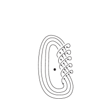
Figure 14: In this formula $d=\gcd(M,N)$, $M=md$ and $N=nd$

9 Examples

We conclude with some explicit special cases of theorem 17, which inspired its general formulation.

Example.  When $M$ and $N$ are coprime then $d=1,m=M$, $n=N$, and so $\Delta_{P_{n}}(P_{m})=\{mn\}T_{m}^{n}$, the framed $(m,n)$ torus link in the solid torus.

Example.  When $N$ is a multiple of $M$ then $d=M,m=1$, $N=Mn$, and so $\Delta_{P_{Mn}}(P_{M})=\{M^{2}n\}T_{1}^{n}*P_{M}$.

In particular where $M=N$, of interest in considering links with all components decorated by $P_{M}$, we have $m=n=1$, $d=M$ and $\Delta_{P_{M}}(P_{M})=\{M^{2}\}T_{1}^{1}*P_{M}$, giving a formula for the effect of the framing change on $P_{M}$ in terms of other links decorated by $P_{M}$ (see figure 15).

$P_{M}$ at 10 266 $P_{M}$ at 340 85 $\ -\$$P_{M}$ at 10 266 $P_{M}$ at 207 120  $=\{M^{2}\}$ $P_{M}$ at 290 450

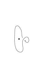
Figure 15: The effect of the framing change on $P_{M}$

Example.  When $M$ is a multiple of $N$, then $d=N,n=1$, $M=mN$ and so $\Delta_{P_{N}}(P_{mN})=\{mN^{2}\}T_{m}^{1}*P_{N}$.

The special case where $N=1$ gives $\Delta_{\varphi}(P_{m})=\Delta_{P_{1}}(P_{m})=\{m\}T_{m}^{1}=v^{-1}\{m\}A_{m}$.

This may be compared with the formula $\Delta_{\overline{\varphi}}(A_{m})=-v\{m\}P_{m}$ obtained in theorem 12, which leads to the formula

$$\Delta_{\overline{\varphi}}\Delta_{\varphi}(P_{m})=-\{m\}^{2}P_{m}.$$

Indeed, lemma 16 shows that $\Delta_{\overline{\varphi}}\Delta_{\varphi}$ operates as the scalar $-\{m\}^{2}$ on the subspace of $\mathcal{C}_{+}$ spanned by $m$-hooks, for each $m$. More generally, $\Delta_{P_{N}^{*}}\Delta_{P_{N}}$ operates as $-\{mN\}^{2}$ on this subspace, where $P_{N}^{*}\in\mathcal{C}$ is $P_{N}$ with the string orientations reversed.

References

- [1] A. K. Aiston, Skein theoretic idempotents of Hecke algebras and quantum group invariants. PhD. thesis, University of Liverpool, 1996.
- [2] A. K. Aiston and H. R. Morton, Idempotents of Hecke algebras of type . J. Knot Theory Ramifications 7 (1998), 463–487.
- [3] Y. M. Chen, A. M. Garsia and J. Remmel, Algorithms for plethysm. Combinatorics and algebra (Boulder, Colo., 1983), 109–153, Contemp. Math. 34 Amer. Math. Soc., Providence, RI, 1984.
- [4] W. Fulton and J. Harris, Representation theory. Graduate texts in mathematics 129, Springer, 1991.
- [5] R. J. Hadji and H. R. Morton, A basis for the full Homfly skein of the annulus. Math. Proc. Camb. Phil. Soc. 141 (2006), 81–100.
- [6] K. Kawagoe, On the skeins in the annulus and applications to invariants of -manifolds. J. Knot Theory Ramifications 7 (1998), 187–203.
- [7] J. M. F. Labastida and M. Mariño, A new point of view in the theory of knot and link invariants. J. Knot Theory Ramifications 11 (2002), 173 –197.
- [8] S. G. Lukac, Homfly skeins and the Hopf link. PhD. thesis, University of Liverpool, 2001.
- [9] S. G. Lukac, Idempotents of the Hecke algebra become Schur functions in the skein of the annulus. Math. Proc. Camb. Phil. Soc. 138 (2005), 79–96.
- [10] I. G. Macdonald, Symmetric functions and Hall polynomials. Clarendon Press, Oxford. Second edition, 1995.
- [11] H. R. Morton, Skein theory and the Murphy operators. J. Knot Theory Ramifications 11 (2002), 475–492.
- [12] H. R. Morton, Power sums and Homfly skein theory. In Geometry and Topology Monographs, Volume 4: Invariants of knots and -manifolds (Kyoto 2001), (2002), 235–244.
- [13] H. Ooguri and C. Vafa, Knot invariants and topological strings. Nuclear Phys. B 577 (2000), 419–438.
- [14] M. Rosso and V. F. R. Jones, On the invariants of torus knots derived from quantum groups. J. Knot Theory Ramifications 2 (1993), 97–112.
- [15] V. G. Turaev, The Conway and Kauffman modules of a solid torus. Zap. Nauchn. Sem. Leningrad. Otdel. Mat. Inst. Steklov. (LOMI) 167, 1988, Issled. Topol. 6, 79–89 (Russian), English translation: J. Soviet Math. 52 (1990), 2799–2805.
- [16] V. G. Turaev, Quantum invariants of knots and 3-manifolds. de Gruyter Studies in Mathematics, 18. Walter de Gruyter and Co., Berlin, 1994.
- [17] H. Wenzl, Representations of braid groups and the quantum Yang-Baxter equation. Pacific J. Math. 145 (1990), 153–180.