Disentanglement of two qubits coupled to an $XY$ spin chain: Role of quantum phase transition

Abstract

We study the disentanglement of two spin qubits which interact with a general XY spin-chain environment. The dynamical process of the disentanglement is numerically and analytically investigated in the vicinity of quantum phase transition (QPT) of the spin chain in both weak and strong coupling cases. We find that the disentanglement of the two qubits is in general enhanced greatly when the environmental spin chain is exposed to QPT. We give a detailed analysis to facilitate the understanding of the QPT-enhanced decaying behavior of the disentanglement factor. Furthermore, the scaling behavior in the disentanglement dynamics is also revealed and analyzed.

The coupling between an entangled quantum system and its environment leads to disentanglement of the system, the process through which quantum information is degraded. Disentanglement is a crucial issue that is of fundamental interest due to the fact that the distributed nonlocal coherence among multi-particles by the entanglement really matters in many important applications of quantum information Preskill ; Nielson . Consequently, the fragility of nonlocal entanglement is recognized as a main obstacle to realizing quantum computing and quantum information processing (QIP) Viola1999 ; Beige2001 . Apart from the important link to QIP realizations, a deeper understanding of disentanglement is also expected to lead new insights into quantum fundamentals, particularly quantum measurement and quantum-classical transitions Dodd . Recently, Yu and Eberly Yu2004 have showed that two entangled qubits become completely disentangled in a finite time under the influence of pure vacuum noise. Zubairy et al. Zubairy have demonstrated how the high quality cavities can be used to realize the new class of quantum erasers referred to as quantum disentanglement erasers. Dodd Dodd has studied the competing effects of environmental noise and interparticle coupling on disentanglement by solving the dynamics of two harmonically coupled oscillators. Cucchietti et al. Cucchietti2005 have considered the decoherence effect of a non-interacting spin chain on a single qubit.

In this paper, we study the disentanglement dynamics of a two-qubit quantum sysmtem. Here, the key point is that we choose a special correlated $XY$ spin chain to model the surrounding environment. This choice of the correlated environment is directly motivated by the recent recognition that the single-qubit decoherence induced by a spin-chain environment displays highly interesting properties Quan ; Cucchietti2007 ; Yuan ; Yi due to the unique occurrence of quantum phase transition (QPT) in the spin-chain environmental subsystem. Quan et al. Quan have studied the transition dynamics of a quantum two-level system from a pure state to a mixed one induced by QPT of the surrounding many-body system. They have shown that the decaying behavior of the Loschmidt echo (LE) is best enhanced by QPT of the surrounding system. Cucchietti et al. Cucchietti2007 have found that the QPT of the spin-chain environment will drive the decay of the quantum coherences in the central quantum system to be Gaussian with a width independent of the system-environment coupling strength.

Motivated by the above-mentioned advances in the QPT effect on the single-qubit decoherence, we turn to study the QPT effect of the environmental spin chain on the two-qubit disentanglement of the central quantum system. The coupled spin system we consider in this paper consists of two quantum subsystems. One subsystem is characterized by two spin-1/2 Hamiltonians, which denotes the general two qubits. We call this subsystem the central system, in the sense that these two spins play the role of measuring disentanglement. Whereas the other subsystem (a general $XY$ spin chain in a transverse magnetic field) plays the role of the many-body environment. Compared to the Ising model which has been recently used to study the QPT effect on the disentanglement Sun2007 , the XY model is parameterized by $\gamma$ and $\lambda$ (see Eq. (1) below). Two distinct critical regions appear in parameter space: the segment $(\gamma,\lambda)=(0,(0,1))$ for the $XX$ spin chain and the critical line $\lambda_{c}=1$ for the whole family of the $XY$ model Sach .

The total Hamiltonian for two central spins transversely coupled to a environmental spin chain, which is described by the one-dimensional $XY$ model, is given by ($\hbar$ is taken to be unity)

$$H =-\sum_{l}^{N}\left(\frac{1+\gamma}{2}\sigma_{l}^{x}\sigma_{l+1}^{x}+\frac{1-\gamma}{2}\sigma_{l}^{y}\sigma_{l+1}^{y}+\lambda\sigma_{l}^{z}\right)$$ (1)

$$-\frac{g}{2}\left(\sigma_{A}^{z}+\sigma_{B}^{z}\right)\sum_{l}^{N}\sigma_{l}^{z}$$

$$\equiv H_{E}^{(\lambda)}+H_{I}.$$

Where $H_{E}^{(\lambda)}$ given by first line in Eq. (1) denotes the Hamiltonian of the environmental spin chain, and $H_{I}$ given by the second line denotes describes the interaction between the central two-qubit spins and the spin chain. The Pauli matrices $\sigma_{A(B)}^{z}$ ($\alpha$=$x,y,z$) and $\sigma_{l}^{\alpha}$ are used to describe the central two-qubit spins and the environmental spin-chain subsystems, respectively. The parameters $\lambda$ characterizes the intensity of the transverse magnetic field, and $\gamma$ measures the anisotropy in the in-plane interaction. It is well known that the $XY$ spin model described by the first line in Eq. (1) encompasses two other well-known spin models: the Ising spin chain with $\gamma$=$1$ and the $XX$ chain with $\gamma$=$0$.

The eigenstates of the operator $(\sigma_{A}^{z}+\sigma_{B}^{z})$ are simply given by

$$|1\rangle =|++\rangle_{AB}\text{, \ }|2\rangle=|--\rangle_{AB},$$ (2)

$$|3\rangle =\frac{1}{\sqrt{2}}(|+-\rangle_{AB}+|+-\rangle_{AB}),$$

$$|4\rangle =\frac{1}{\sqrt{2}}(|+-\rangle_{AB}-|+-\rangle_{AB}),$$

where $|\pm\pm\rangle_{AB}\equiv|\pm\rangle_{A}\otimes|\pm\rangle_{B}$ denote the eigenstates of the product Pauli spin operator $\sigma_{A}^{z}\otimes\sigma_{B}^{z}$ with eigenvalues $\pm 1$. The two-qubit states $|1\rangle$, $|2\rangle$, and $|3\rangle$ are simply spin triplet states with total central spin $\sigma_{AB}=2$, while $|4\rangle$ is singlet state with total central spin $\sigma_{AB}=0$. In terms of these two-spin states, the Hamiltonian (1) is rewritten as

$$H=\sum_{j=1}^{4}|j\rangle\langle j|\otimes H_{E}^{(\lambda_{j})},$$ (3)

where the parameters $\lambda_{j}$ are

$$\lambda_{1(2)}=\lambda\pm g\text{, }\lambda_{3}=\lambda_{4}=\lambda,$$ (4)

and $H_{E}^{(\lambda_{j})}$ is given from $H_{E}^{(\lambda)}$ by the replacement of $\lambda$ with $\lambda_{j}$.

As for quantum criticality in the $XY$ model, there are two universality classes depending on the anisotropy $\gamma$. The critical features are characterized by a critical exponent $\nu$ defined by $\xi\sim|\lambda-\lambda_{c}|^{-\nu}$ with $\xi$ representing the correlation length. For any value of $\gamma$, quantum criticality occurs at a critical magnetic field $\lambda_{c}$=$1$. For the interval $0<\gamma\leq 1$ the model belongs to the Ising universality class characterized by the critical exponent $\nu$=$1$, while for $\gamma$=$0$ the model belongs to the $XX$ universality class with $\nu$=$1/2$ Sach .

Considering the initial state $|\Psi(0)\rangle$=$|\phi_{S}(0)\rangle\otimes|\psi_{E}(0)\rangle$, where $|\phi_{S}(0)\rangle$ is the initial state for the two central spins and $|\psi_{E}(0)\rangle$ is the initial state for the environmental spin chain, then the subsequent time evolution of the coupled spin system is determined by the time evolution operator $U(t)$=$\exp(-iHt)$, $|\Psi(t)\rangle$=$U(t)|\Psi(0)\rangle$. Given $|\Psi(t)\rangle$, the central quantity for our investigation, i.e., the evolved reduced density matrix for the two central spins, will be straightforward to obtain. Thus the key task is to determine the time evolution operator in a maximally compact form. For this purpose, we follow the standard procedure Sach by defining the conventional Jordan-Wigner (JW) transformation

$$\sigma_{l}^{x} =\underset{m<l}{\prod}(1-2a_{m}^{+}a_{m})\left(a_{l}+a_{l}^{+}\right),$$

$$\sigma_{l}^{y} =-i\underset{m<l}{\prod}(1-2a_{m}^{+}a_{m})\left(a_{l}-a_{l}^{+}\right),$$ (5)

$$\sigma_{l}^{z} =1-2a_{l}^{+}a_{l},$$

which maps spins to one-dimensional spinless fermions with creation (annihilation) operators $a_{l}^{+}$ ($a_{l}$). After a straightforward derivation, the projected environmental Hamiltonian becomes

$$H_{E}^{(\lambda_{j})}=-\overset{N}{\underset{l}{\sum}}[(a_{l+1}^{+}a_{l}+a_{l}^{+}a_{l+1})+\gamma(a_{l+1}a_{l}+a_{l}^{+}a_{l+1}^{+})+\lambda_{j}(1-2a_{l}^{+}a_{l})].$$ (6)

Next we introduce Fourier transforms of the fermionic operators described by $d_{k}$=$\frac{1}{\sqrt{N}}\sum_{l}a_{l}e^{-i2\pi lk/N}$ with $k$=$-M,..,M$ and $M$=($N-1)/2$. The Hamiltonian (1) can be diagonalized by transforming the fermion operators to momentum space and then using the Bogoliubov transformation. The final result is

$$H_{E}^{(\lambda_{j})}=\sum_{k}\Omega_{k}^{(\lambda_{j})}(b_{k,\lambda_{j}}^{+}b_{k,\lambda_{j}}-\frac{1}{2}),$$ (7)

where the energy spectrum $\Omega_{k}^{(\lambda_{j})}$ is given by

$$\Omega_{k}^{(\lambda_{j})}=2\sqrt{\left(\epsilon_{k}^{(\lambda_{j})}\right)^{2}+\gamma^{2}\sin^{2}\frac{2\pi k}{N}}$$ (8)

with $\epsilon_{k}^{(\lambda_{j})}$=$\lambda_{j}-\cos\frac{2\pi k}{N}$, and the corresponding Bogoliubov-transformed fermion operators are defined by

$$b_{k,\lambda_{j}}=\cos\frac{\theta_{k}^{(\lambda_{j})}}{2}d_{k}-i\sin\frac{\theta_{k}^{(\lambda_{j})}}{2}d_{-k}^{+}$$ (9)

with angles $\theta_{k}^{(\lambda_{j})}$ satisfying $\cos\theta_{k}^{(\lambda_{j})}$=$2\epsilon_{k}^{(\lambda_{j})}/\Omega_{k}^{(\lambda_{j})}$. It is straightforward to see that the normal mode $b_{k,\lambda_{j}}$ dressed by the system-environment interaction is related to the purely environmental normal mode $b_{k,\lambda}$ by the following identity

$$b_{k,\lambda_{j}}=(\cos\alpha_{k}^{(\lambda_{j})})b_{k,\lambda}-i(\sin\alpha_{k}^{(\lambda_{j})})b_{-k,\lambda}^{+},$$ (10)

where $\alpha_{k}^{(\lambda_{j})}$=$(\theta_{k}^{(\lambda_{j})}-\theta_{k}^{(\lambda)})/2$.

The time evolution operator for the Hamiltonian (3) is then given by

$$U(t)=\sum_{j=1}^{4}|j\rangle\langle j|\otimes U_{E}^{(\lambda_{j})}(t),$$ (11)

where $U_{E}^{(\lambda_{j})}(t)$=$\exp(-iH_{E}^{(\lambda_{j})}t)$ is the projected time evolution operator for the spin chain dressed by the system-environment interaction parameter $\lambda_{j}$.

Suppose that initially the central spins $A$ and $B$ are entangled with each other but not with the spin chain, i.e., at $t$=$0$ the two central spins and the environmental spin chain are assumed to be described by the product state

$$|\Psi_{\text{tot}}(0)\rangle=|\phi\rangle_{AB}\otimes|\psi_{E}\rangle,$$ (12)

where $|\phi\rangle_{AB}$ is the entangled initial state of the two central spins and $|\psi_{E}\rangle$ is the initial state of the environmental spin chain. The evolved reduced density matrix of the central spins is derived to be

$$\rho_{AB}(t) =\text{Tr}_{E}|\Psi_{\text{tot}}(t)\rangle\langle\Psi_{\text{tot}}(t)|$$ (13)

$$=\sum_{j,j^{\prime}=1}^{4}c_{j}c_{j^{\prime}}^{\ast}\langle\psi_{E}|U_{E}^{+(\lambda_{j^{\prime}})}(t)U_{E}^{(\lambda_{j})}(t)|\psi_{E}\rangle|j\rangle\langle j^{\prime}|,$$

where $c_{j}$=$\langle j|\phi\rangle_{AB}$. Equation (13) is our starting point for the following derivation and discussions. It reveals in Eq. (13) that the environmental spin chain only modulates the off-diagonal terms of $\rho_{AB}$ through the “decoherence factor”

$$F(t)=\langle\psi_{E}|U_{E}^{+(\lambda_{j^{\prime}})}(t)U_{E}^{(\lambda_{j})}(t)|\psi_{E}\rangle.$$ (14)

Whereas, the diagonal terms of $\rho_{AB}$ are not influenced by the environment since for $j$=$j^{\prime}$, the decoherence factor remains unity. One can see from Eq. (14) that the decoherence factor reflects the overlap between the two states of the environment obtained by evolving the initial state $|\psi_{E}\rangle$ with two Hamiltonians $H_{E}^{(\lambda_{j})}$ and $H_{E}^{(\lambda_{j^{\prime}})}$, which are different (for $j\neq j^{\prime}$) by the system-dependent parameters $\lambda_{j}$ and $\lambda_{j^{\prime}}$ [see Eq. (7)]. Furthermore, we notice that similar to the single-qubit case, the present decoherence factor $F(t)$ of the two qubits also in some special cases has a form of the Loschmidt echo (or fidelity), which can show universal behavior (with exponential decay) when $H_{E}^{(\lambda_{j})}$ are classically chaotic Hamiltonians Jalabert2001 ; Gorin2006 . The new physical connotation endowed by the special choice of spin-chain environment is QPT, which due to its dynamic hypersensitivity to the perturbation induced by a single qubit as previously investigated Quan ; Cucchietti2007 ; Yuan ; Yi , or two qubits to be studied here, will play a fundamental role in determining the dynamics of the central spin(s) and the corresponding decoherence (disentanglement) behaviors.

Before proceeding the discussion, we would like to point out that the reduced density matrix $\rho_{AB}$ sensitively depends through $F(t)$ on the special choice of the initial central-spin state $|\phi\rangle_{AB}$ and spin-chain state $|\psi_{E}\rangle$. In particular, if $|\phi\rangle_{AB}$ lies in the subspace spanned by $|3\rangle$ and $|4\rangle$ [see Eq. (2)], then there is no dynamic correlation between central spins and spin-chain environment, i.e., $F(t)$=$1$ in this case. Thus we choose the initial state of the central spins to have an entangled form

$$|\phi\rangle_{AB} =a|1\rangle+b|2\rangle$$ (15)

$$=a|++\rangle_{AB}+b|--\rangle_{AB}.$$

As a consequence, the time evolution of the two central spins will be confined within this two-dimensional subspace consisting of $|1\rangle$ and $|2\rangle$ and $\rho_{AB}$ is reduced to a $2\times 2$ matrix. On the other side, the choice of the initial spin-chain state $|\psi_{E}\rangle$ also needs to be mentioned. In the previous work Quan ; Cucchietti2007 ; Yuan ; Yi involving decoherence of single qubit in the spin-chain environment, the qubit is chosen to initially be its unperturbed ground state $|g\rangle$. Then $|\psi_{E}\rangle$ is naturally and simply chosen to be the ground state of the constrained spin-chain Hamiltonian, $H_{g}$=$\langle g|H|g\rangle$. In the present two-qubit case, however, since the initially chosen entangled state $|\phi\rangle_{AB}$ is not the eigenstate of the unperturbed qubits, thus one cannot choose the initial state of the spin chain in the same way as used in the single-qubit discussions. Here we choose the initial state $|\psi_{E}\rangle$ of the environment to be the ground state $|G\rangle_{\lambda}$ of the purely spin-chain Hamiltonian $H_{E}^{(\lambda)}$. This choice of $|\psi_{E}\rangle$ is natural since it may be assumed that the coupling between the central spin subsystem and the spin-chain subsystem is adiabatically applied.

The ground state $|G\rangle_{\lambda}$ of $H_{E}^{(\lambda)}$ is the vacuum of the fermionic modes described by $b_{k,\lambda}|G\rangle_{\lambda}$=$0$, and can be written as $|G\rangle_{\lambda}$=$\prod\nolimits_{k=1}^{M}\left(\cos\frac{\theta_{k}^{(\lambda)}}{2}|0\rangle_{k}|0\rangle_{-k}+i\sin\frac{\theta_{k}^{(\lambda)}}{2}|1\rangle_{k}|1\rangle_{-k}\right)$, where $|0\rangle_{k}$ and $|1\rangle_{k}$ denote the vacuum and single excitation of the $k$th mode $d_{k}$, respectively. Note that the ground state is a tensor product of states, each lying in the two-dimensional Hilbert space spanned by $|0\rangle_{k}|0\rangle_{-k}$ and $|1\rangle_{k}|1\rangle_{-k}$. From the relationship between the Bogoliubov modes $b_{k,\lambda}$ and $b_{k,\lambda_{j}}$ [equation (10)], one can see that the ground state $|G\rangle_{\lambda}$ of the purely spin-chain Hamiltonian $H_{E}^{\lambda}$ can be obtained from the ground state $|G\rangle_{\lambda_{j}}$ of the qubit-dressed Hamiltonian $H_{E}^{\lambda_{j}}$ by the transformation

$$|G\rangle_{\lambda}=\prod\nolimits_{k=1}^{M}(\cos\alpha_{k}^{(\lambda_{j})}+i\sin\alpha_{k}^{(\lambda_{j})}b_{k,\lambda_{j}}^{+}b_{-k,\lambda_{j}}^{+})|G\rangle_{\lambda_{j}}.$$ (16)

Given the initial state $|\Psi_{\text{tot}}(0)\rangle$=$|\phi\rangle_{AB}\otimes|\psi_{E}\rangle$ of the whole system, then our present task is to derive the explicit expression for the decoherence factor $F(t)$. First one notices that $F(t)$ in Eq. (14) can be written as

$$|F(t)| =|_{\lambda}\langle G|U_{E}^{+(\lambda_{2})}(t)U_{E}^{(\lambda_{1})}(t)|G\rangle_{\lambda}|$$ (17)

$$=|_{\lambda_{2}}\langle G|\prod_{k}\left(\cos\alpha_{k}^{(\lambda_{2})}-i\sin\alpha_{k}^{(\lambda_{2})}b_{-k,\lambda_{2}}b_{k,\lambda_{2}}\right)$$

$$\times e^{iH_{E}^{(\lambda_{2})}t}e^{-iH_{E}^{(\lambda_{1})}t}\prod_{k}\left(\cos\alpha_{k}^{(\lambda_{1})}+i\sin\alpha_{k}^{(\lambda_{1})}b_{k,\lambda_{j}}^{+}b_{-k,\lambda_{1}}^{+}\right)|G\rangle_{\lambda_{1}}|.$$

By using the identity $e^{-iH_{\lambda}t}b_{k,\lambda}^{+}e^{iH_{\lambda}t}$=$b_{k,\lambda}^{+}e^{-i\Omega_{k}^{(\lambda)}t}$, Eq. (17) is rewritten as

$$\left|F\left(t\right)\right| =\prod\nolimits_{k>0}|\sin\alpha_{k}^{(\lambda_{1})}\sin\alpha_{k}^{(\lambda_{2})}\cos\left(\alpha_{k}^{(\lambda_{1})}-\alpha_{k}^{(\lambda_{2})}\right)\exp\left(-i\Omega_{k}^{\lambda_{1}}t+i\Omega_{k}^{\lambda_{2}}t\right)$$ (18)

$$-\cos\alpha_{k}^{(\lambda_{1})}\sin\alpha_{k}^{(\lambda_{2})}\sin\left(\alpha_{k}^{(\lambda_{1})}-\alpha_{k}^{(\lambda_{2})}\right)\exp\left(i\Omega_{k}^{\lambda_{1}}t+i\Omega_{k}^{\lambda_{2}}t\right)$$

$$+\sin\alpha_{k}^{(\lambda_{1})}\cos\alpha_{k}^{(\lambda_{2})}\sin\left(\alpha_{k}^{(\lambda_{1})}-\alpha_{k}^{(\lambda_{2})}\right)\exp\left(-i\Omega_{k}^{\lambda_{1}}t-i\Omega_{k}^{\lambda_{2}}t\right)$$

$$+\cos\alpha_{k}^{(\lambda_{1})}\cos\alpha_{k}^{(\lambda_{2})}\cos\left(\alpha_{k}^{(\lambda_{1})}-\alpha_{k}^{(\lambda_{2})}\right)\exp\left(i\Omega_{k}^{\lambda_{1}}t-i\Omega_{k}^{\lambda_{2}}t\right)|.$$

Equation (18) will be used in the latter discussions, one variant of its form, which will also be used for discussion, is the following

$$|F(t)| =\prod\nolimits_{k>0}\{1-\sin^{2}\left(2\alpha_{k}^{(\lambda_{1})}\right)\sin^{2}\left(\Omega_{k}^{(\lambda_{1})}t\right)-\sin^{2}\left(2\alpha_{k}^{(\lambda_{2})}\right)\sin^{2}\left(\Omega_{k}^{(\lambda_{2})}t\right)$$ (19)

$$+2\sin\left(2\alpha_{k}^{(\lambda_{1})}\right)\sin\left(2\alpha_{k}^{(\lambda_{2})}\right)\sin\left(\Omega_{k}^{(\lambda_{1})}t\right)\sin\left(\Omega_{k}^{(\lambda_{2})}t\right)\cos\left(\Omega_{k}^{(\lambda_{1})}t-\Omega_{k}^{(\lambda_{2})}t\right)$$

$$-4\sin\left(2\alpha_{k}^{(\lambda_{1})}\right)\sin\left(2\alpha_{k}^{(\lambda_{2})}\right)\sin^{2}\left(\alpha_{k}^{(\lambda_{1})}-\alpha_{k}^{(\lambda_{2})}\right)\sin^{2}\left(\Omega_{k}^{(\lambda_{1})}t\right)\sin^{2}\left(\Omega_{k}^{(\lambda_{2})}t\right)\}^{\frac{1}{2}}$$

$$\equiv\prod\nolimits_{k>0}F_{k}(t).$$

Equation (19) [or Eq. (18)] is one main result in this paper. It can be simplified under some special conditions. For example, if one chooses the initial spin-chain state to be $|\psi_{E}\rangle$=$|G\rangle_{\lambda_{2}}$, then Eq. (14) and corresponding Eq. (19) will be reduced to a LE form given in Ref. Yuan . It is straightforward to see that each factor $F_{k}$ in Eq. (19) has a norm less than unity, thus one may expect $F(t)$ to decrease to zero in the large $N$ limit under some reasonable conditions. Now we study in detail the critical behavior of the decoherence factor $F(t)$ near the critical point $\lambda_{c}$=$1$ for finite lattice size $N$ of the spin chain. Following Ref. Quan , let us first make a heuristic analysis of the features of $F(t)$. For a cutoff frequency $K_{c}$ we define the partial product for $F(t)$

$$|F_{c}(t)|=\prod\nolimits_{k=1}^{K_{c}}F_{k}\geq|F(t)|,$$ (20)

and the corresponding partial sum $S(t)$=$\ln|F_{c}(t)|\equiv-\sum\nolimits_{k=1}^{K_{c}}|\ln F_{k}|$. For small $k$ and small $g$ (weak coupling) one has

$$\Omega_{k}^{(\lambda)} \approx 2\left|\lambda-1\right|+O(k^{2}),$$ (21)

$$\Omega_{k}^{(\lambda_{j})} \approx 2\left|\lambda_{j}-1\right|+O(k^{2}),$$

and then

$$\sin\left(2\alpha_{k}^{(\lambda_{j})}\right) \approx\frac{\mp 2\gamma\pi kg}{N|(\lambda_{j}-1)(\lambda-1)|},$$ (22)

$$\sin\left(\alpha_{k}^{(\lambda_{1})}-\alpha_{k}^{(\lambda_{2})}\right) \approx\frac{-2\gamma\pi kg}{N|(\lambda_{1}-1)(\lambda_{2}-1)|}.$$

As a result, one has

$$S(t) \approx-\frac{1}{2}E\left(K_{c}\right)\gamma^{2}g^{2}\left(\lambda-1\right)^{-2}\left(\lambda_{1}-1\right)^{-2}$$ (23)

$$\times\left(\lambda_{2}-1\right)^{-2}\{\left(\lambda_{2}-1\right)^{2}\sin^{2}\left(2\left|\lambda_{1}-1\right|t\right)$$

$$+\left(\lambda_{1}-1\right)^{2}\sin^{2}\left(2\left|\lambda_{2}-1\right|t\right)$$

$$-2\left|\left(\lambda_{1}-1\right)\left(\lambda_{2}-1\right)\right|\sin\left(2\left|\lambda_{1}-1\right|t\right)$$

$$\times\sin\left(2\left|\lambda_{2}-1\right|t\right)\cos\left(4\lambda t\right)\},$$

where $E\left(K_{c}\right)=4\pi^{2}K_{c}\left(K_{c}+1\right)\left(2K_{c}+1\right)/\left(6N^{2}\right)$. In the derivation of the above equation, we have omitted the terms related to the sum of $k^{4}/N^{4}$. Consequently, in the short time $t$ one has

$$\left|F_{c}(t)\right|\approx e^{-\tau t^{2}}$$ (24)

when $\lambda\rightarrow\lambda_{c}=1$, where $\tau=8E\left(K_{c}\right)\gamma^{2}g^{2}/\left(\lambda-1\right)^{2}$.

One can see from Eq. (24) that when $N$ is large enough and $\lambda$ $\rightarrow\lambda_{c}=1$, then $\left|F_{c}(t)\right|$ will decay to zero in a short time. It should be noticed that when increasing $N$, the cutoff frequency $K_{c}$ should also linearly increase to remain the validity of Eq. (24). Otherwise, one would derive an unphysical conclusion that in the thermodynamic limit, i.e., the number $N$ of the sites approaching infinite while keeping the length of the spin chain fixed, $\tau$ tends to zero and thus the approximate expression $\left|F_{c}(t)\right|$ remains unity without any decay. Therefore, in using Eq. (24) to reveal the close relationship between the decaying behavior of $\left|F(t)\right|$ and QPT which occur only in the thermodynamic limit, it is necessary to keep the value of $K_{c}/N$ invariant when increasing $N$ to infinity. Such kind of scaling relation will be further revealed in the latter discussions in this paper.

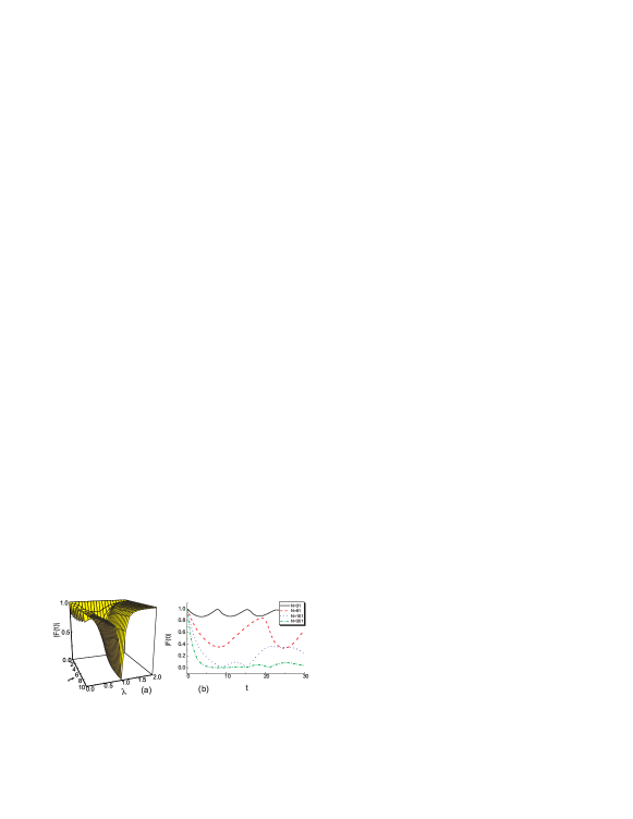
Figure 1: (Color online). (a) Disentanglement factor $|F(t)|$ as a function of magnetic intensity $\lambda$ and time $t$ for two central spin qubits coupled (with coupling strength $g=0.05$) to an Ising ($\gamma=1.0$) spin chain with the size $N=201$. (b) Disentanglement factor for different sizes of Ising spin chain at QPT point ($\lambda=1$).

Now we check the dynamical property of $\left|F(t)\right|$ by numerical analysis calculated from the exact expression Eq. (19). In Fig. 1(a), the $\left|F(t)\right|$ is plotted as a function of magnetic intensity $\lambda$ and time $t$ for $N$=$201$, $g$=$0.05$, and $\gamma$=$1.0$ (i.e., the case of Ising spin chain and in the weak coupling regime). One can see that apart from the critical point $\lambda_{c}$, the $\left|F(t)\right|$ in time domain is characterized by an oscillatory localization behavior. When the amplitude of $\lambda$ approaches to $\lambda_{c}$, the degree of localization of $\left|F(t)\right|$ is decreased to zero. The fundamental change occurs at a critical point of QPT, ie., $\lambda$=$\lambda_{c}$=1. At this point, as revealed in Fig. 1(a), the $\left|F(t)\right|$ evolves from unity to zero in a very short time, which implies that the disentanglement of two central spins is best enhanced by QPT in the environmental spin chain. The size dependence of the decoherence factor is shown in Fig. 1(b) for $\lambda$=$\lambda_{c}$ and $g$=$0.05$. Not surprisingly, with increasing $N$ towards thermodynamic limit, the role of QPT in Ising spin chain becomes clear by completely disentangling the two central qubits in a very short time.

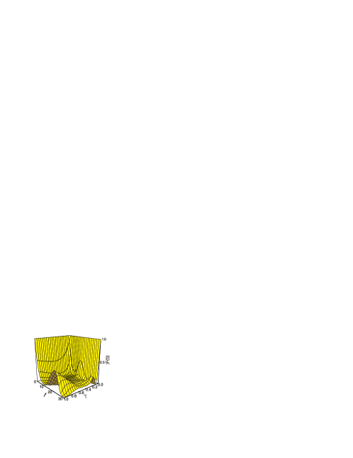
Figure 2: (Color online). Disentanglement factor $|F(t)|$ as a function of spin anisotropy parameter $\gamma$ and time $t$ for two central spin qubits coupled to an XY spin chain. The other parameters are set to be $\lambda=1$, $N=201$, and $g=0.05$.

As mentioned at the beginning of this paper, for the XY model we employed, there are two distinct critical regions in parameter space. Region I is the segment $(\gamma,\lambda)=(0,(0,1))$ for the $XX$ spin chain, while region II is a critical line $\lambda_{c}$=$1$ for the whole family of the $XY$ model (including the special case $\gamma$=$1$ of Ising model). We find that the best-enhancement behavior of the disentanglement factor $\left|F(t)\right|$ only occurs in QPT region II except for the point $(0,1)$. Whereas in the whole region I and at the point $(0,1)$, $\left|F(t)\right|$ remains unity during the time evolution, and thus the QPT in the environmental spin chain has no any effect on the entanglement of the two central spins. This full localization behavior of $\left|F(t)\right|$ can be seen from the analytic expression, Eq. (24), in which $\tau$=$0$ for $\gamma$=$0$, indicating no decay in $\left|F(t)\right|$, regardless of the variation of $\lambda$ and the couping strength $g$. Physically, this vanishing of disentanglement for the two central qubits under an $XX$ spin-chain environment can be seen by noticing that the parameters $\theta_{k}^{(\lambda_{j})}$ and $\theta_{k}^{(\lambda)}$ in Eq. (10) are zero (or $\pi$) at $\gamma$=$0$. In this case, the fermionic modes $b_{k,\lambda_{j}}$ and $b_{k,\lambda}$ coincide each other, which leads to complete overlap between the ground state $|G\rangle_{\lambda_{j}}$ of $H_{E}^{(\lambda_{j})}$ and the ground state $|G\rangle_{\lambda_{j^{\prime}}}$ of $H_{E}^{(\lambda_{j^{\prime}})}$, $|G\rangle_{\lambda_{j}}$=$|G\rangle_{\lambda_{j^{\prime}}}$. As a result, one sees from Eq. (14) that the disentanglement factor $F(t)$ keeps an invariant value of unity during its time evolution. Thus one arrives an important conclusion that the enhancement of the disentanglement by QPT may be broken by special choice of the spin-chain the occurrence of ground-state “accidental” degeneracy among the system-dressed environmental spin-chain Hamiltonians $H_{E}^{(\lambda_{j})}$ in critical parameter space. For further illustration, we show in Fig. 2 $\left|F(t)\right|$ as a function of time and $\gamma$ for $\lambda$=1.0, $N$=201, and $g$=0.05 (weak coupling), which corresponds to critical region II. One can see that with deviating $\gamma$ from zero, the disentanglement factor gradually evolves towards zero in an oscillatory way.

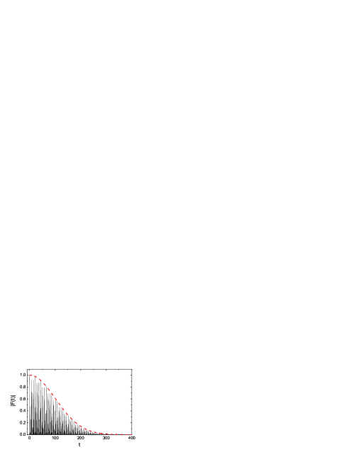
Figure 3: (Color online). Disentanglement factor $|F(t)|$ as a function of time in strong coupling regime. The system parameters are chosen to be $\lambda=1.0$, $N=201$, $\gamma=1.0$, and $g=500.0$. The exact numerical result is shown by solid line, while the approximate Gaussian envelope factor is plotted by dashed line.

After discussing the QPT effect on the disentanglement of two spin qubits in weak coupling regime ($g<<\lambda_{c}$), we turn now to study the QPT effect in strong coupling regime ($g>>\lambda_{c}$). In Fig. 3 (solid line) we display the time evolution of $|F(t)|$ for the values of $\lambda$=1.0, $\gamma$=1.$0$ (Ising model), $N$=$201$, and $g$=$500$. Besides the best-enhancement behavior ($|F(t)|\rightarrow$0 in final time) of the disentanglement as discussed above, one additional prominent new feature, which is absent in the weak coupling case, is that the decay of $|F(t)|$ is now characterized by an oscillatory Gaussian envelope. To explain this, we starts from the observation that when $g\gg 1$, the spin-chain energy spectrum in Eq. (8) can be simplified to $\Omega_{k}^{(\lambda_{1})}\approx 2\epsilon_{k}^{(\lambda_{1})}$ and $\Omega_{k}^{(\lambda_{2})}\approx-2\epsilon_{k}^{(\lambda_{2})}$. Thus from Eq. (9) one has $\theta_{k}^{(\lambda_{1})}\approx 0$ and $\theta_{k}^{(\lambda_{2})}\approx\pi$. This leads to the approximate identity $\alpha_{k}^{(\lambda_{1})}-\alpha_{k}^{(\lambda_{2})}\approx-\pi/2$, by substitution of which into Eq. (18) one can obtain

$$\left|F\left(t\right)\right|\approx\prod\nolimits_{k>0}|\cos^{2}\alpha_{k}^{(\lambda_{1})}\exp\left(i\bar{\Omega}_{k}t\right)+\sin^{2}\alpha_{k}^{(\lambda_{1})}\exp\left(-i\bar{\Omega}_{k}t\right)|,$$ (25)

where $\bar{\Omega}_{k}=\Omega_{k}^{\lambda_{1}}+\Omega_{k}^{\lambda_{2}}$. Remarkably, the above expression for $\left|F\left(t\right)\right|$ is completely analogous to the one found when studying decoherence on a qubit induced by noninteracting spin environment Cucchietti2005 (see Eq. (16) in Ref. Cucchietti2005 ). Thus, one can exactly follow the mathematical derivation given in Ref. Cucchietti2005 and Ref. Cucchietti2007 . The resultant approximate expression for $\left|F\left(t\right)\right|$ is as follows

$$\left|F\left(t\right)\right|\approx\exp\left(-s_{N}^{2}t^{2}/2\right)\left|\cos(\Omega t)\right|^{(N-1)/2},$$ (26)

where $\Omega$ is the mean value of $\bar{\Omega}_{k}$, i.e., $\Omega$=$\frac{1}{M}\sum_{k>0}\bar{\Omega}_{k}$, and

$$s_{N}^{2}=\sum_{k>0}\sin^{2}2\alpha_{k}^{(\lambda_{1})}\delta_{k}^{2}.$$ (27)

Here the quantity $\delta_{k}$ describes the deviation of $\bar{\Omega}_{k}$ from its mean value $\Omega$. It is straightforward to obtain $\Omega\approx 4g+\gamma^{2}/g$ and $\delta_{k}\approx-\frac{\gamma^{2}}{g}\cos\frac{4\pi k}{N}$. We remark that the present Gaussian character of the disentanglement factor is not only confined to the QPT regime. Here it is mainly for purpose of the consistency in organizing this paper that we focus our attention to the strongly coupling behavior of $\left|F\left(t\right)\right|$ in the vicinity of QPT. After a careful analysis of Eq. (27), we further find that the width of the Gaussian envelope is proportional to $g\gamma^{-2}N^{-1/2}$, which is an important scaling relation between the decaying factor $\left|F\left(t\right)\right|$ and the system parameters in the strong coupling QPT regime. For comparison with the exact numerical result, we also show in Fig. 3 (dashed line) the Gaussian envelope factor $\exp\left(-s_{N}^{2}t^{2}/2\right)$ in the approximate expression (26) of $\left|F\left(t\right)\right|$. Clearly, the agreement is very good, indicating the validity of our approximation in QPT region ($\lambda$=$1$ for Ising model) with strong system-environment interaction.

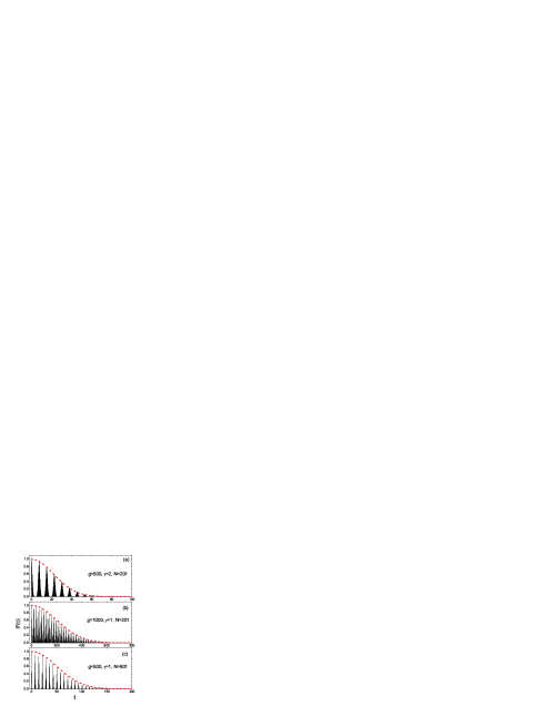
Figure 4: (Color online). Disentanglement factor $|F(t)|$ as a function of time in strong coupling QPT regime ($\lambda=1.0$) for different choices of parameters $\gamma$, $g$ and $N$ to show their relationships with the decaying width of $|F(t)|$. Again, the exact numerical result is shown by solid line, while the approximate Gaussian envelope factor is plotted by dashed line.

Figures 4(a)-(c) display the exactly numerical results (solid lines) of $\left|F\left(t\right)\right|$ and the analytic results (dashed lines) of Gaussian envelope factor $\exp\left(-s_{N}^{2}t^{2}/2\right)$ for $\lambda$=$1$ and different choices of the other parameters $g$, $\gamma$, and $N$. It remarkably reveals in Fig. 4 that the decaying width of $|F(t)|$ is proportional to the product $g\gamma^{-2}N^{-1/2}$, exactly as we have analyzed in the above discussions.

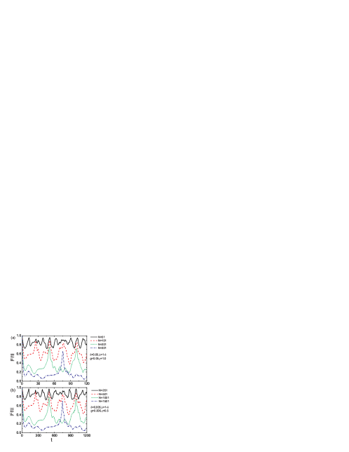
Figure 5: (Color online). Scaling behavior of $|F(t)|$ in the vicinity of the critical point $\lambda_{c}$=$1$ in the weak coupling case. The parameters used in plotting curves in (b) are related to those used in plotting curves (with the same curve type) in (a) by the transformation $g$ $\rightarrow\alpha g$, $\delta\rightarrow\alpha\delta$, $\gamma/N\rightarrow\alpha\gamma/N$ with $\alpha=0.1$. One can see that by further transformation $t\rightarrow t/\alpha$, figures (a) and (b) will completely overlap.

Finally, we find that in the vicinity of QPT, the shape of the disentanglement factor $\left|F\left(t\right)\right|$ during its time evolution is invariant under the scaling transformation $t\rightarrow t/\alpha$, $\delta\rightarrow\alpha\delta$, $g\rightarrow\alpha g$, and $\gamma/N\rightarrow\alpha\gamma/N$, where $\delta=\lambda_{c}-\lambda$ characterizes the vicinity of QPT. To illustrate this remarkable scaling property, we plot in Figs. 5 the exact numerical results of evolution of $|F(t)|$ for different values of the system parameters. Here the values of the system parameters used in Fig. 5(b) are obtained from those used in Fig. 5(a) by a scaling factor $\alpha=0.1$. Clearly, it shows in Fig. 5 that the exact time evolution of $\left|F\left(t\right)\right|$ faithfully follow this scaling transformation. Remarkably, the similar scaling property has been recently found Quan in studying dynamics of the LE for a single qubit coupled to an Ising-type spin chain. Clearly, this scaling rule in the disentanglement factor $|F(t)|$ for two entangled qubits or in the LE for the single qubit is highly meaningful in quantum computing and quantum information processing.

To understand this scaling property, here we give a detailed analysis of the behavior of $|F(t)|$ in the vicinity of the critical point $\lambda_{c}$=$1$ in the case of weak coupling strength $g$. Note that although in the present context we only concern the specific model employed in this paper, the following analysis can be easily applied to the other cases. We first notice that in the expression of $|F(t)|$ [Eq. (19)], most factors $F_{k}$ remains nearly unity. Thus only very few $F_{k}$’s have remarkable effect on the shape and amplitude of $|F(t)|$. From Eq (19) one can see that in order for the factor $F_{k}$ to deviate prominently from unity, at least one of its two coefficients $\sin 2\alpha_{k}^{(\lambda_{j})}$ ($j=1,2$) should be considerably non-zero. Next let us check the value of $\sin 2\alpha_{k}^{(\lambda_{j})}$. For this we define $k_{c}^{(\lambda_{j})}$ which enables $\left|\epsilon_{k_{c}}^{(\lambda_{j})}\right|$=$\left|\lambda_{j}-\cos\left(2\pi k_{c}^{(\lambda_{j})}/N\right)\right|$ as small as possible. For small $\delta$ (i.e., $\lambda-\lambda_{c}$) and $g$, one can see that $k_{c}^{(\lambda_{j})}\ll M$. From the definition of $\alpha_{k}^{(\lambda_{j})}$, we can write down

$$\sin 2\alpha_{k}^{(\lambda_{j})}=\mp 4\gamma g\sin\left(2\pi k/N\right)/\Omega_{k}^{(\lambda_{j})}\Omega_{k}^{\lambda}$$ (28)

for $j=1$, 2, respectively. One can see from Eq. (28) and the expressions of $\Omega_{k}^{(\lambda_{j})}$ and $\Omega_{k}^{\lambda}$ that for small $g$, to enable $\sin 2\alpha_{k}^{(\lambda_{j})}$ considerably non-zero, three conditions should be satisfied: (i) $k$ should be close to $k_{c}^{(\lambda_{j})}$ and $k_{c}^{(\lambda)}$ in order for the amplitude of $\gamma\sin\left(2\pi k/N\right)$ to be comparable with $\epsilon_{k_{c}}^{(\lambda_{j})}$ and $\epsilon_{k_{c}}^{(\lambda)}$; (ii) $g$ is small enough so that $k$ could be close to $k_{c}^{(\lambda_{j})}$ and $k_{c}^{(\lambda)}$ at the same time. (iii) $\delta$ is small which leads to small value of $\sin\left(2\pi k/N\right)$ when $k$ approaching $k_{c}^{(\lambda_{j})}$ and $k_{c}^{(\lambda)}$. Under these three conditions, one has the following approximate expressions

$$\Omega_{k}^{(\lambda_{j})} \approx 2\left[\left(\delta\mp g\right)^{2}+4\gamma^{2}\pi^{2}k^{2}/N^{2}\right]^{1/2},$$ (29)

$$\Omega_{k}^{\lambda} \approx 2\left(\delta^{2}+4\gamma^{2}\pi^{2}k^{2}/N^{2}\right)^{1/2}.$$

Combining Eq. (28) and Eq. (29), one immediately finds that the transformation $g$ $\rightarrow\alpha g$, $\delta\rightarrow\alpha\delta$, and $\gamma/N\rightarrow\alpha\gamma/N$ leads to $\Omega_{k}^{(\lambda_{j})}\rightarrow\alpha\Omega_{k}^{(\lambda_{j})}$, $\Omega_{k}^{\lambda}\rightarrow\alpha\Omega_{k}^{\lambda}$, while $\sin 2\alpha_{k}^{(\lambda_{j})}$ and $\cos 2\alpha_{k}^{(\lambda_{j})}$ remaining invariant. As a result, the time evolution of $|F(t)|$ in Eq. (19) is well invariant under further transformation $t\rightarrow t/\alpha$. This is what one has seen from the exact results in Fig. 5.

In summary, we have studied the dynamic process of the disentanglement of a coupled system consisting of two spin qubits and a general XY spin chain. The exact expression of the disentanglement factor $|F(t)|$ has been obtained. The relation between $|F(t)|$ and the QPT in the environmental spin chain has been extensively illustrated. It has been shown that in general, the disentanglement of the two qubits is best enhanced when the environmental spin chain is exposed to QPT in either strong or weak coupling case. Both the heuristic analysis and numerical calculations have shown the sharply decaying behavior of the decoherence factor in the vicinity of the critical line $\lambda$=$\lambda_{c}$=$1$. This decaying behavior, on the other side, has been found to break for the particular XX spin chain ($\gamma=0$), in which case $|F(t)|$ is not influenced by the environment. In the strong coupling case, it has been numerically and analytically found that in the vicinity of QPT the disentanglement factor decays to zero in an oscillatory Gaussian envelope. The width of the Gaussian envelope has been found to scale with a form $g\gamma^{-2}N^{-1/2}$. Furthermore, we have established a scaling rule for the time evolution of the disentanglement factor in the vicinity of QPT. We expect that the present results may shed light on the role of strongly correlated environment played in the disentanglement dynamics of multi-qubits.

ZY and SL were supported by NSFC under Grant No. 60325416 and 60521001. PZ was supported by NSFC under Grant Nos. 10604010 and 10544004.

References

• (1) J. Preskill, Lecture Notes on Quantum Information and Quantum Computation at www.theory.caltech.edu/people/preskill/ph229.
• (2) M.A. Nielson and I.L. Chuang, Quantum Computation and Quantum Information (Cambridge University, Cambridge, England, 2000).
• (3) L. Viola, E. Knill, and S. Lloyd, Phys. Rev. Lett. 83, 4888 (1999).
• (4) A. Beige, D. Braun, B. Tregenna, and P.L. Knight, Phys. Rev. Lett. 85, 1762 (2001).
• (5) P.J. Dodd and J.J. Halliwell, Phys. Rev. A 69, 052105 (2004); P.J. Dodd, Phys. Rev. A 69, 052106 (2004).
• (6) T. Yu and J.H. Eberly, Phys. Rev. Lett. 93, 140404 (2004).
• (7) M.S. Zubairy, G.S. Agarwal, and M.O. Scully, Phys. Rev. A 70, 012316 (2004).
• (8) F.M. Cucchietti, J.P. Paz, and W.H. Zurek, Phys. Rev. A 72, 052113 (2005).
• (9) H.T. Quan, Z. Song, X.F. Liu, P. Zanardi, and C.P. Sun, Phys. Rev. Lett. 96, 140604 (2006).
• (10) F.M. Cucchietti, S.F. Vidal, and J.P. Paz, Phys. Rev. A 75, 032337 (2007).
• (11) Z.-G. Yuan, P. Zhang, and S.-S. Li, Phys. Rev. A 75, 012102 (2007).
• (12) X.X. Yi, H. Wang, and W. Wang, e-print cond-mat/0601318.
• (13) Z. Sun, X. Wang, and C.P. Sun, e-print arXiv: quant-ph/0704.1172v1.
• (14) S. Sachdev, Quantum Phase Transition (Cambridge University Press, Cambridge, 1999).
• (15) R.A. Jalabert and H.M. Pastawski, Phys. Rev. Lett. 86, 2490 (2001).
• (16) T. Gorin, T. Prosen, T.H. Seligman, and M. Znidaric, Phys. Rep. 435, 33 (2006); T. Prosen and M. Znidaric, J. Phys. A 35, 1455 (2002).