Multimedia Capacity Analysis of the IEEE 802.11e Contention-based Infrastructure Basic Service Set ^†

Abstract

We first propose a simple mathematical analysis framework for the Enhanced Distributed Channel Access (EDCA) function of the recently ratified IEEE 802.11e standard. Our analysis considers the fact that the distributed random access systems exhibit cyclic behavior. The proposed model is valid for arbitrary assignments of AC-specific Arbitration Interframe Space (AIFS) values and Contention Window (CW) sizes and is the first that considers an arbitrary distribution of active Access Categories (ACs) at the stations. Validating the theoretical results via extensive simulations, we show that the proposed analysis accurately captures the EDCA saturation performance. Next, we propose a framework for multimedia capacity analysis of the EDCA function. We calculate an accurate station- and AC-specific queue utilization ratio by appropriately weighing the service time predictions of the cycle time model for different number of active stations. Based on the calculated queue utilization ratio, we design a simple model-based admission control scheme. We show that the proposed call admission control algorithm maintains satisfactory user-perceived quality for coexisting voice and video connections in an infrastructure BSS and does not present over- or under-admission problems of previously proposed models in the literature.

I Introduction

The IEEE 802.11 standard [1] defines the Distributed Coordination Function (DCF) which provides best-effort service at the Medium Access Control (MAC) layer of the Wireless Local Area Networks (WLANs). The recently ratified IEEE 802.11e standard [2] specifies the Hybrid Coordination Function (HCF) which enables prioritized and parameterized Quality-of-Service (QoS) services at the MAC layer, on top of DCF. The HCF combines a distributed contention-based channel access mechanism, referred to as Enhanced Distributed Channel Access (EDCA), and a centralized polling-based channel access mechanism, referred to as HCF Controlled Channel Access (HCCA). In this paper, we confine our analysis to the EDCA scheme, which uses Carrier Sense Multiple Access with Collision Avoidance (CSMA/CA) and slotted Binary Exponential Backoff (BEB) mechanism as the basic access method. The EDCA defines multiple Access Categories (AC) with AC-specific Contention Window (CW) sizes, Arbitration Interframe Space (AIFS) values, and Transmit Opportunity (TXOP) limits to support MAC-level QoS [2].

We first propose a simple analytical model in order to assess the performance of EDCA function accurately for the saturation (asymptotic) case when each contending AC always has a packet in service (each AC is always active). The analysis of the saturation provides in-depth understanding and insights into the random access schemes and the effect of different contention parameters on the performance. Moreover, as we will show, the saturation figures can effectively be used in network capacity estimation. Our analysis is based on the fact that a random access system exhibits cyclic behavior. A cycle time is defined as the duration in which an arbitrary tagged user successfully transmits one packet on average [3]. We derive the explicit mathematical expression of the station- and AC-specific EDCA cycle time. The derivation considers the AIFS and CW differentiation by employing a simple average collision probability analysis. Our formulation is also the first to consider the scenario such that the number of active ACs may vary from station to station. As a direct result, the proposed model also takes the internal collisions into account in the case of a station having more than one active ACs. We use the EDCA cycle time to predict the average throughput and the average service time in saturation. We show that the results obtained using the cycle time model closely follow the accurate predictions of the previously proposed more complex analytical models and simulation results. Our cycle time analysis can serve as a simple and practical alternative model for EDCA saturation performance analysis.

Due to its contention-based nature, EDCA cannot provide parameterized QoS for realtime applications that require strict QoS guarantees, if the network load and parameters are not tuned such that the network is operating in nonsaturated state [4],[5]. Although the use of an admission control algorithm is recommended in [2] to limit the network load for QoS provision, no algorithm is specified. A loose capacity estimation is harmful for admission control, since the quality of ongoing flows will be jeopardized. Conversely, an underestimation of the network capacity results in fewer number of admitted flows than the network can support.

Rather than designing a new and complex access model with a large number of states in order to calculate the EDCA capacity (in nonsaturation), we propose a novel, simple, and accurate framework which directly employs the results of the proposed simple saturation analysis. An approximate station- and AC-specific average service time is calculated by weighing the average service time calculated using cycle time model for different number of active stations. Given the average station- and AC-specific traffic load, the average service time is directly translated into a station- and AC-specific queue utilization ratio (note that since all the measures are station- and AC-specific, the proposed framework considers the potential unbalanced traffic load in the 802.11e BSS uplink and downlink). Next, we design a novel centralized EDCA admission control algorithm the admission decisions of which are based on the queue utilization ratio. The key point is that the delay guarantee of realtime applications is only possible when the queue utilization ratio of active multimedia flows is smaller than 1 (i.e., when the MAC queue is stable). Comparing the theoretical results with simulations, we show that the proposed call admission control algorithm maintains satisfactory user-perceived quality for coexisting voice and video connections in an infrastructure BSS by limiting the maximum number of admitted flows of each multimedia traffic type. Comparison with extensive simulation results also reveals that the proposed analysis does not result in an overestimation or a significant underestimation of the network capacity. Another attractive feature of the proposed scheme is that it fully complies with the 802.11e standard.

The main contributions of this paper are three-fold; i) a simple average cycle time model to evaluate the performance of the EDCA function in saturation for an arbitrary assignment of AC-specific AIFS and CW values and an arbitrary distribution of active ACs at the stations, ii) an approximate capacity estimation framework which weighs the saturation service times in order to calculate the nonsaturation service time, and iii) a practical model-based admission control algorithm to limit the number of admitted realtime multimedia flows in the 802.11e infrastructure BSS.

II EDCA Overview

The IEEE 802.11e EDCA is a QoS extension of IEEE 802.11 DCF. The major enhancement to support QoS is that EDCA differentiates packets using different priorities and maps them to specific ACs that are buffered in separate queues at a station. Each AC_i within a station ($0\leq i\leq i_{max}$, $i_{max}=3$ in [2]) having its own EDCA parameters contends for the channel independently of the others. Following the convention of [2], the larger the index $i$ is, the higher the priority of the AC is. Levels of services are provided through different assignments of the AC specific EDCA parameters; AIFS, CW, and TXOP limits.

If there is a packet ready for transmission in the MAC queue of an AC, the EDCA function must sense the channel to be idle for a complete AIFS before it can start the transmission. The AIFS of an AC is determined by using the MAC Information Base (MIB) parameters as

$$AIFS=SIFS+AIFSN\times T_{slot},$$ (1)

where $AIFSN$ is the AC-specific AIFS number, $SIFS$ is the length of the Short Interframe Space and $T_{slot}$ is the duration of a time slot.

If the channel is idle when the first packet arrives at the AC queue, the packet can be directly transmitted as soon as the channel is sensed to be idle for AIFS. Otherwise, a backoff procedure is completed following the completion of AIFS before the transmission of this packet. A uniformly distributed random integer, namely a backoff value, is selected from the range $[0,W]$. The backoff counter is decremented at the slot boundary if the previous time slot is idle. Should the channel be sensed busy at any time slot during AIFS or backoff, the backoff procedure is suspended at the current backoff value. The backoff resumes as soon as the channel is sensed to be idle for AIFS again. When the backoff counter reaches zero, the packet is transmitted in the following slot.

The value of $W$ depends on the number of retransmissions the current packet experienced. The initial value of $W$ is set to the AC-specific $CW_{min}$. If the transmitter cannot receive an Acknowledgment (ACK) packet from the receiver in a timeout interval, the transmission is labeled as unsuccessful and the packet is scheduled for retransmission. At each unsuccessful transmission, the value of $W$ is doubled until the maximum AC-specific $CW_{max}$ limit is reached. The value of $W$ is reset to the AC-specific $CW_{min}$ if the transmission is successful, or the retry limit is reached thus the packet is dropped.

The higher priority ACs are assigned smaller AIFSN. Therefore, the higher priority ACs can either transmit or decrement their backoff counters while lower priority ACs are still waiting in AIFS. This results in higher priority ACs enjoying a relatively faster progress through backoff slots. Moreover, the ACs with higher priority may select backoff values from a comparably smaller CW range. This approach prioritizes the access since a smaller CW value means a smaller backoff delay before the transmission.

Upon gaining the access to the medium, each AC may carry out multiple frame exchange sequences as long as the total access duration does not go over a TXOP limit. Within a TXOP, the transmissions are separated by SIFS. Multiple frame transmissions in a TXOP can reduce the overhead due to contention. A TXOP limit of zero corresponds to only one frame exchange per access.

An internal (virtual) collision within a station is handled by granting the access to the AC with the highest priority. The ACs with lower priority that suffer from a virtual collision run the collision procedure as if an outside collision has occured [2].

III Related Work

In this section, we provide a brief summary of the studies in the literature that are related to this work.

III-A Performance Analysis of EDCA in Saturation

Three major saturation performance models have been proposed for DCF; i) assuming constant collision probability for each station, Bianchi [6] developed a simple Discrete-Time Markov Chain (DTMC) and the saturation throughput is obtained by applying regenerative analysis to a generic slot time, ii) Cali et al. [7] employed renewal theory to analyze a p-persistent variant of DCF with persistence factor p derived from the CW, and iii) Tay et al. [8] instead used an average value mathematical method to model DCF backoff procedure and to calculate the average number of interruptions that the backoff timer experiences. Having the common assumption of slot homogeneity (for an arbitrary station, constant collision or transmission probability at an arbitrary slot), these models define all different renewal cycles all of which lead to accurate saturation performance analysis. These major methods (especially [6]) are modified by several researchers to include an accurate treatment of the QoS features of the EDCA function (AIFS and CW differentiation among ACs) in the saturation analysis [9, 10, 11, 12, 13, 14, 15, 16, 17, 18, 19].

Our approach in this paper is based on the observation that the transmission behavior in the contention-based 802.11 WLAN follows a pattern of periodic cycles. Previously, Medepalli et al. [3] provided explicit expressions for average DCF cycle time and system throughput. Similarly, Kuo et al. [19] calculated the EDCA transmission cycle assuming equal collision probability for any AC. On the other hand, such an assumption is shown to lead to analytical inaccuracies [9, 10, 11, 12, 13, 14, 15, 16, 17, 18]. One of the main contributions of this paper is that we incorporate accurate AIFS and CW differentiation calculation in the EDCA cycle time analysis. We show that the cyclic behavior is observed on a per AC per station basis in the EDCA. To maintain the simplicity of the cycle time analysis, we employ averaging on the AC- and station-specific collision probability. Another key contribution of the proposed model is that our analysis is the first analytical EDCA model to consider the possibility of the number of active ACs varying from station to station. The comparison with more complex and detailed theoretical and simulation models reveals that the analytical accuracy is preserved when average cyclic time analysis is used.

III-B Capacity Analysis and Admission Control in EDCA

The Markov analysis of [6] is also modified by several researchers to include the capacity analysis of the DCF or EDCA function in nonsaturation [20, 21, 22, 23]. A number of queueing models have also been proposed to analyze delay performance of a station or an AC under the assumption that the traffic is uniformly distributed [4, 5, 24, 25]. Some other queueing models also assumed a MAC queue size of one packet to define a Markovian framework for performance analysis [26, 27].

There are also studies on capacity analysis and admission control considering the infrastructure BSS where the AP usually has a higher load in the downlink than the stations serving traffic in the uplink. A group of studies mainly concentrated on capacity analysis of only Voice-over-IP traffic for DCF and did not consider traffic differentiation [28, 29, 30, 31, 32, 33]. Gao et al. [34] and Cheng et al. [35] calculated VoIP capacity of the WLAN when CW differentiation among uplink and downlink flows are used. Another group of studies defines parameter adaptation algorithms for QoS enhancement and defines measurement-assisted call admission control algorithms [36, 37, 38, 39, 40, 41, 42].

Being a very simple extension of the proposed cycle time analysis, our approach in this paper provides an accurate multimedia traffic capacity estimation in the case of traffic differentiation between voice, video, and best-effort flows in the WLAN. Our analysis considers the unbalanced traffic between the AP and the stations. Under the motivation of previous findings that the optimum operating point of the 802.11 WLAN lies in nonsaturation [5], we define a simple test for centralized admission control of multimedia traffic based on queue utilization estimates of a simple model. Comparison with simulation results for a broad range of traffic types and load shows that the proposed method provides an accurate network capacity estimation and the proposed admission control algorithm prevents both over- and under-admission problems of previously proposed models.

IV EDCA Cycle Time Analysis

We propose an average cycle time analysis to model the behavior of the EDCA function of any AC at any station. In this section, we will first define a Traffic Class (TC). Then, we will derive the TC-specific average collision probability. Next, we will calculate the TC-specific average cycle time. Finally, we will relate the average cycle time and the average collision probability to the normalized throughput and service time.

The main assumption for saturation analysis is that each AC always has a frame in service. Note that the performance of EDCA differs depends on the number of active ACs within the same station as well as the number of active ACs at the other stations due to the fact that the EDCA function acts differently in the case of an internal or an external collision. One of the key differences of our theoretical formulation from the previous work in the literature is as follows. We consider both the possibility of a station running multiple ACs (thus the possibility of internal collisions) and the possibility of the number of active ACs varying from station to station. For example, consider a simple WLAN scenario where an Access Point (AP, labeled $STA_{0}$ in the sequel) runs 2 downlink ACs, namely AC₁ and AC₂. Similarly, assume $n_{1}$ stations ($STA_{1},\ldots,STA_{n_{1}}$, $n_{1}>0$) only run AC₁ and $n_{2}$ other stations ($STA_{n_{1}+1},\ldots,STA_{n_{1}+n_{2}}$, $n_{2}>0$) only have AC₂ in the uplink. Although there are 2 distinct ACs active in the system, the downlink AC_i and the uplink AC_i ($i=\{1,2\}$ for the running example) cannot be expected to have the same performance due to internal and external collision differentiation [2]. In this case, the performance analysis should be carried out individually for 4 different Traffic Classes (TCs) which are uplink AC₁, downlink AC₁, uplink AC₂, and downlink AC₂.

We make the following mathematical definitions for the sake of the analysis in the sequel.

• Let $\delta_{k}$ ($0\leq k\leq n_{STA}$) be a vector of size 4 which denotes the activity status of ACs at $STA_{k}$ where $n_{STA}$ is the total number of stations that have at least one active AC. The value at dimension $i$ of $\delta_{k}$ shows whether AC_i is active or not at $STA_{k}$. The entries corresponding to the indices of active (inactive) ACs are labeled with 1 (0). In the example above, $\delta_{0}=(0,1,1,0)$, $\delta_{1}=(0,1,0,0)$, $\delta_{n_{1}+1}=(0,0,1,0)$, etc.

• Let $\zeta$ be the set of $\delta_{k}$, i.e., $\zeta=\{\delta_{k}:0\leq k\leq n_{STA}\}$. Above, $\zeta=\{(0,1,0,0),(0,0,1,0),(0,1,1,0)\}$.

• Let $\psi_{i}$ be the set of $\delta_{k}$ where AC_i is active, i.e., $\psi_{i}=\{\delta_{k}:\delta_{k}(i)=1,0\leq k\leq n\}$. In the example above, $\psi_{1}=\{(0,1,0,0),(0,1,1,0)\}$, $\psi_{2}=\{(0,0,1,0),(0,1,1,0)\}$, and $\psi_{0}=\psi_{3}=\{\}$.

• Let $N(S)$ be an operator on a set $S$ which shows the number of elements in the set. Then, the total number of TCs with AC_i active are $N(\psi_{i})$ and the total number of TCs is $J=\sum_{i=0}^{i=3}N(\psi_{i})$. Note that $N(\zeta)\leq J$ should always hold. In the sequel, each distinct TC is denoted by TC_j ($0\leq j<J$). We also define $\sigma_{j}$ as the activity status vector of TC_j. In the example above, $N(\zeta)=3$ and $J=4$. TC₀ is the AC₁ when only AC₁ is active at the station ($\sigma_{1}=\psi_{1}(1)$). TC₁ is the AC₁ with both AC₁ and AC₂ are active ($\sigma_{2}=\psi_{1}(2)$). TC₂ is the AC₂ when only AC₂ is active at the station ($\sigma_{3}=\psi_{2}(1)$). TC₃ is the AC₂ with both AC₁ and AC₂ are active ($\sigma_{4}=\psi_{2}(2)$).

• Let $F$ be a function with the domain of indices of TCs and the range of indices of ACs. We define this function such as the image of the argument $j$ under function $F$ is the index $i$ of the AC that TC_j uses, i.e., $F(j)=\{i:TC_{j}\in\psi_{i}\}$.

• Let $G$ be a function from the domain of the indices of TCs to the range of sets of indices of TCs. We define this function such as the image of the argument $j$ under mapping $G$ is the set of TC indices $j^{\prime}$ with the same $\sigma$, i.e., $G(j)=\{\forall j^{\prime}:\sigma_{j}=\sigma_{j^{\prime}},0\leq j^{\prime}<J\}$.

IV-A TC-specific Average Collision Probability

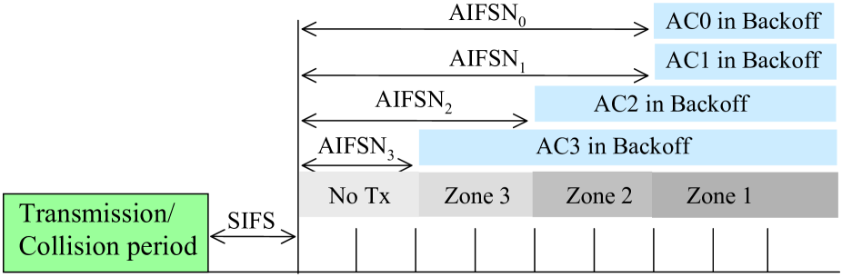
Figure 1: EDCA backoff after busy medium.

The difference in AIFS of each AC in EDCA creates the so-called contention zones or periods as shown in Fig. 1 [11],[12]. In each contention zone, the number of contending TCs may vary. In order to be consistent with the notation of [2], we assume $AIFS_{0}\geq AIFS_{1}\geq AIFS_{2}\geq AIFS_{3}$. Let $d_{j}=AIFSN_{F(j)}-AIFSN_{3}$. Also, let $n^{th}$ backoff slot after the completion of $AIFS_{3}$ idle interval following a transmission period be in contention zone $x$. Then, we define $x=\max\left(F(y)~{}|~{}d_{y}=\underset{z}{\max}(d_{z}~{}|~{}d_{z}\leq n)\right)$ which shows contention zone label $x$ is assigned the largest index value within a set of ACs that have the largest AIFSN value which is smaller than or equal to $n+AIFSN_{3}$.

We define $p_{c_{j,x}}$ ($0\leq j<J$) as the conditional probability that TC_j experiences either an external or an internal collision in contention zone $x$. Note $AIFS_{x}\geq AIFS_{F(j)}$ should hold for TC_j to transmit in zone $x$. Following the slot homogeneity assumption of [6], assume that each TC_j transmits with constant probability, $\tau_{j}$. Also, let the total number TC_j flows be $f_{j}$. Then,

$$p_{c_{j,x}}=1-\frac{\prod\limits_{\forall j^{\prime}:d_{j^{\prime}}\leq d_{F^{-1}(x)}}(1-\tau_{j^{\prime}})^{f_{j^{\prime}}}}{\prod\limits_{\forall j^{\prime}\in G(j):F(j^{\prime})\leq F(j)}(1-\tau_{j})}.$$ (2)

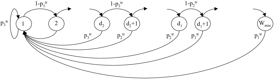
Figure 2: Transition through backoff slots in different contention zones for the example given in Fig.1.

We use the Markov chain shown in Fig. 2 to find the long term occupancy of the contention zones. Each state represents the $n^{th}$ backoff slot after the completion of the AIFS₃ idle interval following a transmission period. The Markov chain model uses the fact that a backoff slot is reached if and only if no transmission occurs in the previous slot. Moreover, the number of states is limited by the maximum idle time between two successive transmissions which is $W_{min}=\min(CW_{F(j),max})$ for a saturated scenario. The probability that at least one transmission occurs in a backoff slot in contention zone $x$ is

$$p^{tr}_{x}=1-\prod_{\forall j^{\prime}:d_{j^{\prime}}\leq d_{F^{-1}(x)}}(1-\tau_{j^{\prime}})^{f_{j^{\prime}}}.$$ (3)

Note that $F^{-1}$ is not one-to-one. Therefore, we define the image of $F^{-1}(i)$ as a randomly selected TC index $j$ which satisfies $F(j)=i$.

Given the state transition probabilities as in Fig. 2, the long term occupancy of the backoff slots $b^{\prime}_{n}$ can be obtained from the steady-state solution of the Markov chain. Then, the TC-specific average collision probability $p_{c_{j}}$ is found by weighing zone specific collision probabilities $p_{c_{j,x}}$ according to the long term occupancy of contention zones (thus backoff slots)

$$p_{c_{j}}=\frac{\sum_{n=d_{j}+1}^{W_{min}}p_{c_{j,x}}b^{\prime}_{n}}{\sum_{n=d_{j}+1}^{W_{min}}b^{\prime}_{n}}.$$ (4)

where $x$ is calculated depending on the value of $n$ as stated previously.

IV-B TC-Specific Average Cycle Time

Let $E_{j}[t_{cyc}]$ be average cycle time for a tagged TC_j user. $E_{j}[t_{cyc}]$ can be calculated as the sum of average duration for i) the successful transmissions, $E_{j}[t_{suc}]$, ii) the collisions, $E_{j}[t_{col}]$, and iii) the idle slots, $E_{j}[t_{idle}]$ in one cycle.

$$E_{j}[t_{cyc}]=E_{j}[t_{suc}]+E_{j}[t_{col}]+E_{j}[t_{idle}]$$ (5)

In order to calculate the average time spent on successful transmissions during a TC_j cycle time, we should find the expected number of total successful transmissions between two successful transmissions of TC_j. Let $Q_{j}$ represent this random variable. Also, let $\gamma_{j}$ be the probability that the transmitted packet belongs to an arbitrary user from TC_j given that the transmission is successful. Then,

$$\gamma_{j}=\frac{\sum_{n=d_{j}+1}^{W_{min}}b^{\prime}_{n}p_{s_{j,n}}/f_{j}}{\sum_{n=d_{j}+1}^{W_{min}}(b^{\prime}_{n}\sum\limits_{\forall l}p_{s_{l,n}})}$$ (6)

where

$$p_{s_{j,n}}=\left\{\\ \begin{IEEEeqnarraybox}[]{[}][c]{lc}\frac{f_{j}\tau_{j}\prod_{j^{\prime}:d_{j^{\prime}}\leq n-1}(1-\tau_{j^{\prime}})^{f_{j^{\prime}}}}{\prod_{\forall j^{\prime}\in G(j):F(j^{\prime})\leq F(j)}(1-\tau_{j})},&~{}{\rm if}~{}n\geq d_{j}+1\\ 0,&~{}{\rm if}~{}n<d_{j}+1.\end{IEEEeqnarraybox}\right.$$ (7)

Then, the Probability Mass Function (PMF) of $Q_{j}$ is

$$Pr(Q_{j}=k)=\gamma_{j}(1-\gamma_{j})^{k},~{}~{}k\geq 0.$$ (8)

We can calculate the expected number of successful transmissions of any TC${}_{j^{\prime}}$ during the cycle time of TC_j, $ST_{j^{\prime},j}$, as

$$ST_{j^{\prime},j}=f_{j^{\prime}}E[Q_{j}]\frac{\gamma_{j^{\prime}}}{1-\gamma_{j}}.$$ (9)

Inserting $E[Q_{j}]=(1-\gamma_{j})/\gamma_{j}$ in (9), the intuition that each user from TC_j can transmit successfully once on average during the cycle time of another TC_j user, i.e., $ST_{j,j}=f_{j}$, is confirmed. Including the own successful packet transmission time of tagged TC_j user in $E_{j}[t_{suc}]$, we find

$$E_{j}[t_{suc}]=\sum_{\forall j^{\prime}}ST_{j^{\prime},j}T_{s_{j^{\prime}}}$$ (10)

where $T_{s_{j^{\prime}}}$ is defined as the time required for a successful packet exchange sequence (will be derived in (18)).

To obtain $E_{j}[t_{col}]$, we need to calculate the average number of users who are involved in a collision, $f_{c_{n}}$, at the $n^{th}$ slot after last busy time for given $f_{j}$ and $\tau_{j}$, $\forall j$. Let the total number of users transmitting at the $n^{th}$ slot after last busy time be denoted as $Y_{n}$. We see that $Y_{n}$ is the sum of random variables, $Binomial(f_{j},\tau_{j})$, $\forall j:~{}d_{j}\leq n-1$. Employing simple probability theory, we can calculate $f_{c_{n}}=E[Y_{n}|Y_{n}\geq 2]$. After some algebra and simplification,

$$f_{c_{n}}=\frac{\sum\limits_{j:d_{j}\leq n-1}(f_{j}\tau_{j}-p_{s_{j,n}})}{1-\prod\limits_{j:d_{j}\leq n-1}(1-\tau_{j})^{f_{j}}-\sum\limits_{j:d_{j}\leq n-1}p_{s_{j,n}}}$$ (11)

If we let the average number of users involved in a collision at an arbitrary backoff slot be $f_{c}$, then

$$f_{c}=\sum_{\forall n}b^{\prime}_{n}f_{c_{n}}.$$ (12)

We can also calculate the expected number of collisions that an TC${}_{j^{\prime}}$ user experiences during the cycle time of a TC_j, $CT_{j^{\prime},j}$, as

$$CT_{j^{\prime},j}=\frac{p_{c_{j^{\prime}}}}{1-p_{c_{j^{\prime}}}}ST_{j^{\prime},j}.$$ (13)

Then, defining $T_{c_{j^{\prime}}}$ as the time wasted in a collision period (will be derived in (19)),

$$E_{j}[t_{col}]=\frac{1}{f_{c}}\sum_{\forall j^{\prime}}CT_{j^{\prime},j}T_{c_{j^{\prime}}}.$$ (14)

Given $p_{c_{j}}$, we can calculate the expected number of backoff slots $E_{j}[t_{bo}]$ that TC_j waits before attempting a transmission. Let $W_{i,k}$ be the CW size of AC_i at backoff stage $k$ [14]. Note that, when the retry limit $r_{i}$ is reached, any packet is discarded. Therefore, another $E_{j}[t_{bo}]$ passes between two transmissions with probability $p_{c_{j}}^{r_{i}}$ (where $i=F(j)$).

$$E_{j}[t_{bo}]=\frac{1}{1-p_{c_{j}}^{r_{i}}}\sum_{k=1}^{r_{i}}p_{c_{j}}^{k-1}(1-p_{c_{j}})\frac{W_{i,k}}{2}.$$ (15)

Noticing that between two successful transmissions, AC_j also experiences $CT_{j,j}$ collisions,

$$E_{j}[t_{idle}]=E_{j}[t_{bo}](CT_{j,j}/f_{j}+1)t_{slot}.$$ (16)

The transmission probability of a user using TC_j is

$$\tau_{j}=\frac{1}{E_{j}[t_{bo}]+1}.$$ (17)

Note that, in [12], it is proven that the mean value analysis for the average transmission probability calculated as in (17) matches the Markov analysis of [6].

The equations (2)-(4), (15), and (17) are a set of nonlinear equations which can be solved numerically for $\tau_{j}$ and $p_{c_{j}}$, $\forall j$. Then, the average cycle time for AC_j, $\forall j$, can be calculated using (5) where each term in (5) is obtained via (6)-(16).

IV-C Performance Analysis

Let $T_{p_{j}}$ be the average payload transmission time for TC_j ($T_{p_{j}}$ includes the transmission time of MAC and PHY headers), $\delta$ be the propagation delay, $T_{ack}$ be the time required for acknowledgment packet (ACK) transmission. Then, for the basic access scheme, we define the time spent in a successful transmission $T_{s_{j}}$ and a collision $T_{c_{j}}$ for any TC_j as

$$T_{s_{j}}= T_{p_{j}}+\delta+SIFS+T_{ack}+\delta+AIFS_{F(j)}$$ (18)

$$T_{c_{j}}= T_{p^{*}_{j}}+ACK\_Timeout+AIFS_{F(j)}$$ (19)

where $T_{p^{*}_{j}}$ is the average transmission time of the longest packet payload involved in a collision [6]. For simplicity, we assume the packet size to be equal for any TC, then $T_{p^{*}_{j}}=T_{p_{j}}$. Being not explicitly specified in the standards, we set $ACK\_Timeout$, using Extended Inter Frame Space (EIFS) as $EIFS_{i}-AIFS_{i}$ ($i=F(j)$). Note that the extensions of (18) and (19) for the RTS/CTS scheme are straightforward [6].

The average cycle time of an TC represents the renewal cycle for each TC. Then, the normalized throughput of TC_j is defined as the successfully transmitted information per renewal cycle

$$S_{j}=\frac{f_{j}T_{p_{j}}}{E_{j}[t_{cyc}]}.$$ (20)

The TC-specific cycle time is directly related but not equal to the mean protocol service time. By definition, the cycle time is the duration between successful transmissions. We define the average protocol service time such that it also considers the service time of packets which are dropped due to retry limit. On the average, $1/p_{j,drop}$ service intervals correspond to $1/p_{j,drop}-1$ cycles (where $p_{j,drop}=p_{c_{j}}^{r_{i}}$ is the average packet drop probability). Therefore, the mean service time $E_{j}[t_{srv}]$ can be calculated as

$$E_{j}[t_{srv}]=(1-p_{j,drop})E_{j}[t_{cyc}].$$ (21)

IV-D Validation

We validate the accuracy of the numerical results by comparing them to the simulation results obtained from ns-2 [43]. For the simulations, we employ the IEEE 802.11e HCF MAC simulation model for ns-2.28 [44]. This module implements all the EDCA and HCCA functionalities stated in [2].

In simulations, we consider two ACs, one high priority (AC₃) and one low priority (AC₁). Unless otherwise is stated, each station runs only one AC. For both ACs, the payload size is 1000 bytes. RTS/CTS handshake is turned on. The simulation results are reported for the wireless channel which is assumed to be not prone to any errors during transmission. The errored channel case is left for future study. All the stations have 802.11g Physical Layer (PHY) using 54 Mbps and 6 Mbps as the data and basic rate respectively ($T_{slot}=9~{}\mu s$, $SIFS=10~{}\mu s$) [45]. The simulation runtime is 100 seconds.

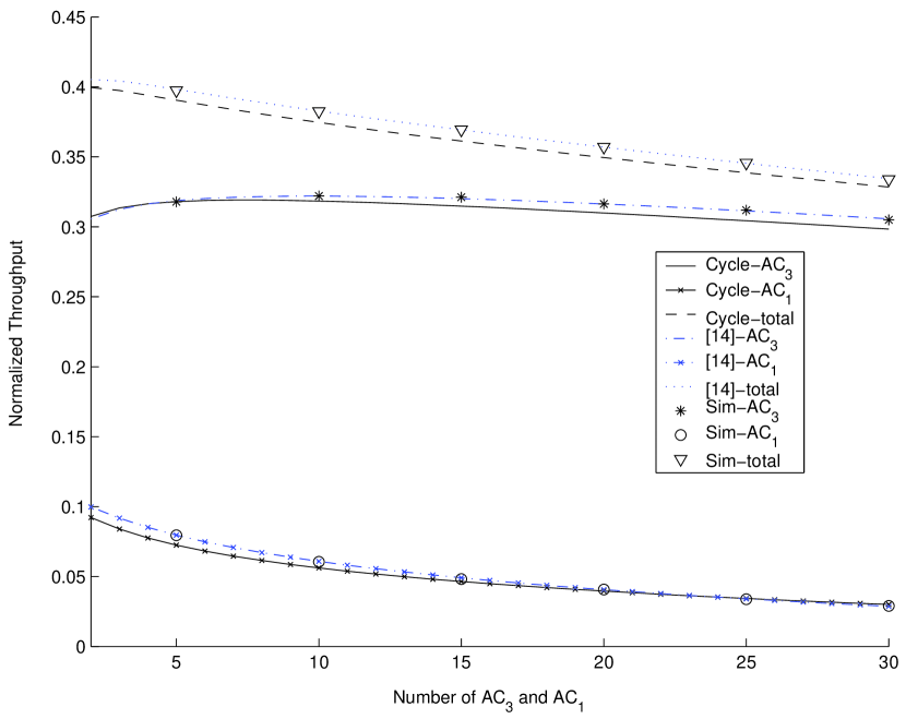
Figure 3: Analyzed and simulated normalized throughput of each AC when both $N_{1}$ and $N_{3}$ are varied from 5 to 30 and equal to each other for the cycle time analysis. Analytical results of the model proposed in [14] are also added for comparison.

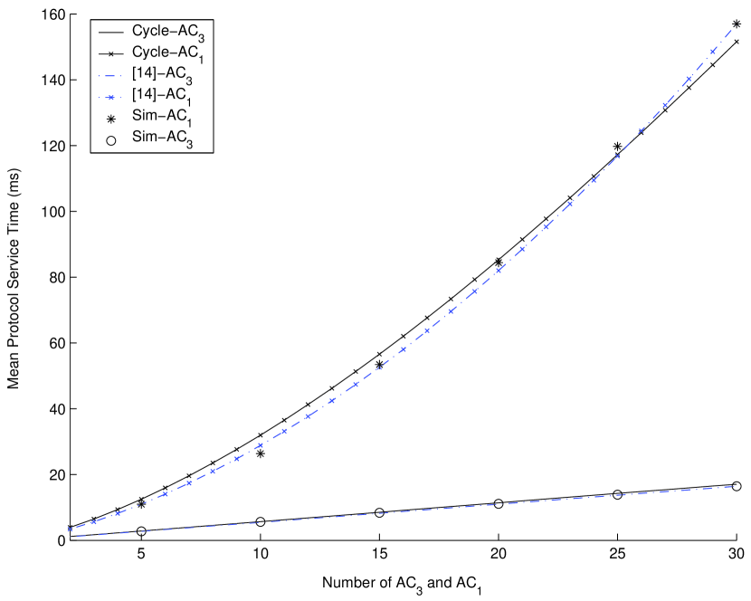
Figure 4: Analyzed and simulated mean protocol service time of each AC when both $N_{1}$ and $N_{3}$ are varied from 5 to 30 and equal to each other for the proposed cycle time analysis and the model in [14].

In the first set of experiments, we set $AIFSN_{1}=3$, $AIFSN_{3}=2$, $CW_{1,min}=31$, $CW_{3,min}=15$, $m_{1}=m_{3}=3$, $r_{1}=r_{3}=7$. Fig. 3 shows the normalized throughput of each AC when both $N_{1}$ and $N_{3}$ are varied from 5 to 30 and equal to each other. As the comparison with a more detailed analytical model [14] and the simulation results reveal, the cycle time analysis can predict saturation throughput accurately. Fig. 4 displays the mean protocol service time for the same scenario of Fig. 3. As comparison with [14] and the simulation results show, the mean protocol service time can accurately be predicted by the proposed cycle time model. Although not included in the figures, a similar discussion holds for the comparison with other detailed and/or complex models of [15]-[17] and for other performance metrics such as mean packet drop probability.

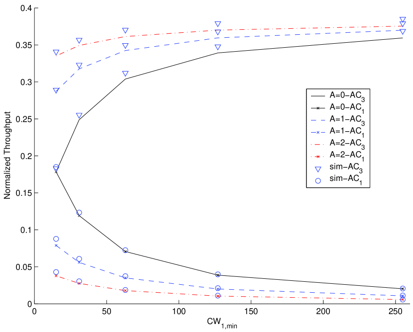
Figure 5: Analytically calculated and simulated performance of each AC when $AIFSN_{3}=2$, $CW_{3,min}=15$, $N_{1}=N_{3}=10$, $AIFSN_{1}$ varies from 2 to 4, and $CW_{1,min}$ takes values from the set $\{15,31,63,127,255\}$. Note that $AIFSN_{1}-AIFSN_{3}$ is denoted by $A$.

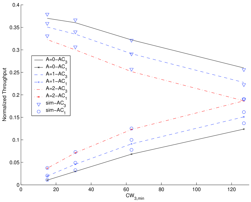
Figure 6: Analytically calculated and simulated performance of each AC when $AIFSN_{1}=4$, $CW_{1,min}=127$, $N_{1}=N_{3}=10$, $AIFSN_{3}$ varies from 2 to 4, and $CW_{3,min}$ takes values from the set $\{15,31,63,127\}$. Note that $AIFSN_{1}-AIFSN_{3}$ is denoted by $A$.

In the second set of experiments, we fix the EDCA parameters of one AC and vary the parameters of the other AC in order to show the proposed cycle time model accurately captures the normalized throughput for different sets of EDCA parameters. In the simulations, both $N_{1}$ and $N_{3}$ are set to 10. Fig. 5 shows the normalized throughput of each AC when we set $AIFSN_{3}=2$, $CW_{3,min}=15$, and vary $AIFSN_{1}$ and $CW_{1,min}$. Fig. 6 shows the normalized throughput of each AC when we set $AIFSN_{1}=4$, $CW_{1,min}=127$, and vary $AIFSN_{3}$ and $CW_{3,min}$. As the comparison with simulation results show, the predictions of the proposed cycle time model are accurate. Although, we do not include the results for packet drop probability and service time for this experiment, no discernable trends toward error are observed.

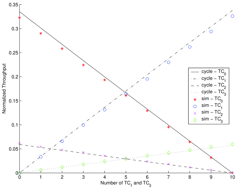
Figure 7: Analytically calculated and simulated performance of each TC when the number of TC₁ and TC₃ is varied from 0 to 10 (therefore, TC₀ and TC₂ vary from 10 to 0).

In the third set of experiments, we test the performance of the system when the stations run multiple ACs so that virtual collisions may occur. The stations run only AC₁, only AC₃, or both. Like in Section IV, we define TC₀ as the AC₃ when only AC₃ is active at the station, TC₁ the AC₃ when both AC₃ and AC₁ are active at the station, TC₂ as the AC₁ when only AC₁ is active at the station, and TC₃ the AC₁ when both AC₃ and AC₁ are active at the station. We keep both $N_{1}$ and $N_{3}$ at 10, and vary the number of TC₁ and TC₃ from 0 to 10 (therefore, TC₀ and TC₂ vary from 10 to 0). Fig. 7 shows the normalized throughput of each TC. The predictions of the proposed analytical model follow the simulation results closely. Although not significant for the tested scenario and not apparent in the graphical results, a closer look on the numerical results present the (slightly) higher level of differentiation between AC₃ and AC₁ which is due to the additional prioritization introduced at the virtual collision procedure.

V Multimedia Capacity Analysis for 802.11e Infrastructure BSS

When working in the saturated case, the contention-based 802.11 MAC suffers from a large collision probability, which leads to low channel utilization and excessively long delay. As shown in [5], the optimal operating point for the 802.11 to work lies in nonsaturation where contention-based 802.11 MAC can achieve maximum throughput and small delay. In [46], it is also shown that a very small increase in system load yields a huge increase (of about two orders of magnitude) of the backoff delay. When the traffic load does not exceed the service rate at saturation, the resulting medium access delay is very small.

In this section, we propose a novel framework where we calculate TC-specific average frame service rate $\mu$ via a weighted summation of saturation service rate $E[t_{srv}]$ over varying number of active stations. Defining a TC-specific average queue utilization ratio $\rho$, we design a simple call admission control algorithm which limits the number of admitted real-time multimedia flows in the 802.11e infrastructure BSS in order to prevent the corresponding TC queues going into saturation. As specified in [2], the admission control is conducted at the AP. Admitted real-time multimedia flows can be served with QoS guarantees, since low transmission delay and packet loss rate can be maintained when the 802.11e WLAN is in nonsaturation [5],[46]. Comparing with simulation results, we show that not only does the proposed admission control algorithm prevent the so-called over-admission or under-admission problems but also efficiently utilizes the network capacity.

V-A TC-specific Average Queue Utilization Ratio

Each station runs a QoS reservation procedure with the AP for all of its traffic streams that need parameterized (guaranteed) QoS support. The Station Management Entity (SME) at the AP decides whether the Traffic Stream (TS) is admitted or not regarding the Traffic Specification (TSPEC) in the Add Traffic Stream (ADDTS) request provided by the station. The TSPEC specifies the Traffic Stream Identification Number ($TSID$), the user priority ($UP$), the mean data rate ($R$), and the mean packet size ($L$) of the corresponding TS [2].

Let average frame service rate for TC_j be denoted as $\mu_{j}$. Also let the average packet arrival rate for TC_j be denoted as $\lambda_{j}$ which can easily be calculated employing $R$ of TSs using the same TC at the same station. For simplicity, in the sequel, we assume that TCs at different stations are running TSs with equal TSPEC values (so all traffic parameters remain TC-specific). Though all work in this section can be generalized for varying traffic load and parameters within a TC vary at different stations, we opted not to present this out-of-scope generalization since it would make the model difficult to understand.

We define TC-specific queue utilization ratio $\rho$ as follows

$$\rho_{j}=\lambda_{j}/\mu_{j},~{}\forall j.$$ (22)

V-B TC-specific Average Frame Service Rate

The TC-specific average queue utilization ratio $\rho_{j}$ shows the percentage of time on average that TC_j has a frame in service. In other words, $\rho_{j}$ is the probability that TC_j is active. Our novel approach in calculating $\mu_{j}$ is forming a weighted summation of $E_{j}[t_{srv}]$ for varying number of active TCs.

Let $P_{TC_{0},TC_{1},...,TC_{j},...,TC_{J-1}}^{j}(f^{\prime}_{0},f^{\prime}_{1},...,f^{\prime}_{j},...,f^{\prime}_{J-1})$ denote the joint conditional probability that $f^{\prime}_{j}$ stations using TC_j, $\forall j$, are active given that one TC_j has a frame in service and the total number of TCs is $J$. Also, let $E_{j}[t_{srv}(f^{\prime}_{0},f^{\prime}_{1},...,f^{\prime}_{J-1})]$ denote the average service time when $f^{\prime}_{j}$ stations using TC_j, $\forall j$, are active. We use the proposed cycle time model in Section IV to calculate $E_{j}[t_{srv}(f^{\prime}_{0},f^{\prime}_{1},...,f^{\prime}_{J-1})]$. Then, the TC-specific average frame service rate $\mu_{j}$ is calculated as follows

$$\frac{1}{\mu_{j}}=\sum_{0\leq f^{\prime}_{0}\leq f_{0}}...\sum_{1\leq f^{\prime}_{j}\leq f_{j}}...\sum_{0\leq f^{\prime}_{J-1}\leq f_{J-1}}E_{j}[t_{srv}(f^{\prime}_{0},...,f^{\prime}_{j},...,f^{\prime}_{J-1})]\cdot P_{TC_{0},...,TC_{j},...,TC_{J-1}}^{j}(f^{\prime}_{0},...,f^{\prime}_{j},...,f^{\prime}_{J-1}).$$ (23)

Note that the case when $\sum_{j^{\prime}=0}^{J-1}f^{\prime}_{j^{\prime}}=1$, i.e., there is only one active TC, is not considered by the proposed cycle time model. On the other hand, the cycle time calculation in this case is straightforward. Since no collisions can occur and no other station is active, the successful transmission is performed at AIFS completion. Therefore, $E_{j}[t_{srv}(f^{\prime}_{0},f^{\prime}_{1},...,f^{\prime}_{J-1})]=T_{s_{j}}$ if $\sum_{j^{\prime}=0}^{J-1}f^{\prime}_{j^{\prime}}=1$.

We noticed that the distribution of the number of active TCs approximates the sum of independent Binomial distributions with parameters $f_{j^{\prime}}$ and $\rho_{j^{\prime}}$, $\forall j^{\prime}$ as in (24) for the traffic models we used in this study. We confirm the validity of (24) via comparing the analytical estimations with simulation results in Section V-D. On the other hand, we do not argue that the binomial activity distribution holds for any type of traffic model in any scenario. Our observation is that for widely used voice and video traffic models this approximation works well. The proposed framework is generic in the sense that any other activity distribution profile may be used to incorporate other traffic models in other network scenarios.

$$P_{TC_{0},TC_{1},...,TC_{j},...,TC_{J-1}}^{j}(f^{\prime}_{0},f^{\prime}_{1},...,f^{\prime}_{j},...,f^{\prime}_{J-1})=\dbinom{f_{j}-1}{f^{\prime}_{j}-1}\rho_{j}^{f^{\prime}_{j}-1}(1-\rho_{j})^{f_{j}-f^{\prime}_{j}}\prod_{\forall j^{\prime}:j^{\prime}\neq j}\dbinom{f_{j^{\prime}}}{f^{\prime}_{j^{\prime}}}\rho_{j^{\prime}}^{f^{\prime}_{j^{\prime}}}(1-\rho_{j^{\prime}})^{f_{j^{\prime}}-f^{\prime}_{j^{\prime}}}$$ (24)

The fixed-point equations (22)-(24) can numerically be solved for $\rho_{j}$ and $\mu_{j}$, $\forall j$.

V-C Admission Control Procedure

Upon receiving the ADDTS request, the AP associates the TS with the AC and the TC using the value in the $UP$ field and the station MAC address. The traffic stream is admitted if and only if the following tests succeed

$$\rho_{j}\leq\rho_{th},~{}\forall j.$$ (25)

where $\rho_{th}\leq 1$. The tests in (25) ensure that the average traffic arrival rate to all TCs is smaller than the average service rate that can be provided to them. Therefore, the MAC queues of all TCs can be considered to be stable (all TCs remain in nonsaturation on average).

When a real-time flow ends, the source node transmits a Delete Traffic Stream (DELTS) request for the TS [2]. The AP deletes the corresponding entry from the list of admitted flows.

A few remarks on admission control and capacity analysis are as follows.

• The proposed capacity analysis and admission control scheme can easily be extended to the case where some TCs are running best-effort traffic. We actually do a worst-case analysis in Section V-D where the TCs that run best-effort traffic are assumed to be always active. This generalizes (23) as

  $$\frac{1}{\mu_{j}}=\sum_{0\leq f^{\prime}_{1}\leq f_{1}}...\sum_{1\leq f^{\prime}_{j}\leq f_{j}}...\sum_{0\leq f^{\prime}_{J^{\prime}}\leq f_{J^{\prime}}}E_{j}[t_{srv}(f^{\prime}_{1},...,f^{\prime}_{j},...,f^{\prime}_{J^{\prime}-1},f_{J^{\prime}},...,f_{J-1})]\cdot P_{TC_{1},...,TC_{J^{\prime}}}^{j}(f^{\prime}_{1},...,f^{\prime}_{J^{\prime}})$$ (26)

  where $J^{\prime}$ and $J-J^{\prime}$ are the number of TCs that run multimedia and best-effort flows respectively. In this case, the admission control tests in (25) are done for TCs that run real-time flows, i.e., $0\leq j\leq J^{\prime}$.

• Although the employed saturation model does not consider wireless channel errors, the admission control scheme can still be effective in an error-prone wireless channel as the admission control decisions are threshold-based. Selecting a comparably smaller $\rho_{th}<1$ can provide the necessary room for packet retransmissions occuring as a result of wireless channel losses. This may be a more simpler approach when compared to a solution that includes the design of a more complex saturation analysis model considering wireless channel errors. The investigation is left as future work.

• The proposed capacity estimation scheme is solely based on mean values and do not consider the worst-case scenario where all the admitted Variable Bit Rate (VBR) multimedia traffic may instantaneously transmit at their peak rate ($R_{peak}$). Again a wise decision $\rho_{th}$ can limit the channel utilization by multimedia flows thereby leaving room to accommodate bandwidth fluctuations caused by VBR traffic. Alternatively, $R_{peak}$ may be used in the calculation of $\lambda$ in (22). On the other hand, when $R_{peak}/R$ is very large, this may result in the rejection of many multimedia flows and unnecessarily low channel utilization.

• The TSPECs may also specify a Delay Bound ($DB$) which denotes the maximum time allowed to transport the frames across the wireless interface including the queueing delay [2]. As also provided in [5, Table I], multimedia services should satisfy QoS requirements in terms of one-way transmission delay, delay variation, and packet loss rate. For example, for voice and video the excellent (acceptable) quality is satisfied if the delay is smaller than 150 ms (400 ms) and the packet loss rate is smaller than $1\%-3\%$ [5]. Note that packet loss rate includes the dropped packets at the playout buffer of the receiver when the packets are not received within the delay bound. Our capacity analysis does not explicitly consider these metrics in admission control. On the other hand, the proposed call admission control algorithm makes the multimedia TC queues remain stable (TC queues do not go into saturation) by limiting the number of admitted real-time flows. This provides low transmission delays and packet loss ratio due to the low collision probability in nonsaturation [5].

• In the simulations, we observed that the delay experienced by multimedia flows in nonsaturation can go up to 40-50 ms depending on the scenario. In order to guarantee a stochastic delay bound, the admission control tests in (25) should be extended. We may use the method proposed in [35]

  $${\rm Pr}(Q_{j}>DB_{j}\cdot\mu_{j})\leq\epsilon$$ (27)

  where $Q_{j}$ is the queue length of the TC_j and $\epsilon$ is the delay violation probability. This test can be extended further for on/off traffic sources and statistical multiplexing at the AP as shown in [35]. On the other hand, in the simulation scenarios we have studied, the addition of this test does not limit the already admitted traffic using (25) since the QoS requirements of the multimedia flows are always satisfied if the system is in nonsaturation state.

• In the simulations, we consider two types of traffic sources; voice and video, where the average packet size of different traffic sources vary. Therefore, $T_{c}$ is not equal for any TC since $T_{p_{j}^{*}}=T_{p_{j}}$ does not always hold. Due to space limitations, we do not include the calculation of $T_{c_{j}}$ in this case. We use the method in [6] which has an extensive treatment of the subject.

V-D Validation

For the experiments, we use a network topology such that any connection is initiated between a distinct party in the Internet and the WLAN. The traffic is relayed at the AP from (to) the wireless channel to (from) the wired link. The simulations consider three types of traffic sources; voice, video, and background data. The voice traffic models G.711 or G.729 VoIP application as Constant Bit Rate (CBR) traffic (without the use of silence suppression scheme). The CBR traffic model is used for two reasons; i) it provides a worst-case upper bound for the case when the traffic presents on-off traffic characteristics (silence suppression) and ii) this enables comparison of voice capacity results with the models proposed in [28, 29, 30, 31, 32, 33, 34]. The parameters of the VoIP codecs are set as in [33, Table I]. For the video source models, we use the traces of real MPEG-4 video streams [47]. For the particular video source used in the simulations presented in this paper, the average codec bit rate is 174 kbps with an average packet size of 821 bytes. Real-time packets have 40-byte length RTP/UDP/IP header. The background data traffic is modeled by bulk data transfer where every AC using this type of traffic is saturated. Voice flows use AC₃, video flows use AC₂, and background traffic uses AC₁. We set the EDCA parameters as suggested in [2]; $AIFSN_{3}=3$, $AIFSN_{2}=2$, $AIFSN_{3}=2$, $CW_{1,min}=31$, $CW_{2,min}=15$, $CW_{3,min}=7$, $CW_{1,max}=1023$, $CW_{2,max}=31$, $CW_{3,max}=15$, $r=7$. PHY parameters are set as stated in Section IV-D. The wired link delay is set to 20 ms for all connections.

V-D1 Voice Capacity Analysis

In the first set of experiments, we investigate the VoIP capacity of 802.11e WLAN when no other type of traffic coexists. A two-way voice connection is established every $\omega$ ms, with the starting time randomly chosen over $[0,\omega]$ ms. We set $\omega$ equal to the packet interval duration of the voice codec used. Table I tabulates the maximum number of admitted VoIP connections for different codecs. In the simulations, the maximum number of voice connections is obtained in such a way that one more connection results in a packet loss ratio larger than $1\%$. As shown in Table I, the analytical results for the proposed model and the simulation results closely follow each other. As the comparison of the performance with 802.11e MAC parameters in 802.11g PHY layer indicates, the model in [33] has significant under-admission problems for an arbitrary selection of MAC parameters (especially when the CW settings are small and the underlying PHY is 802.11g). We do not provide any comparison with [30, 31, 32] the over-admission problems of which are already shown in [33].

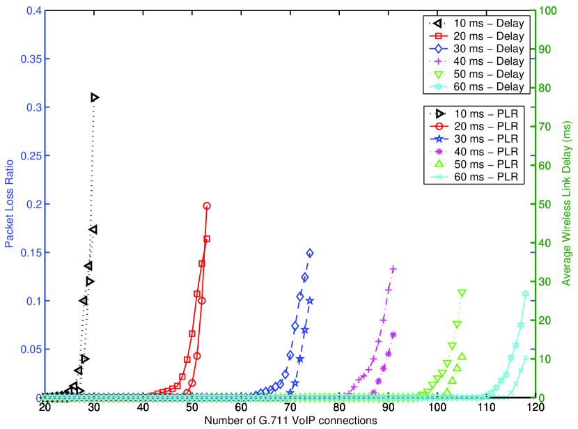
Figure 8: Packet loss ratio and average delay in the downlink for increasing number G.711 VoIP connections.

Fig. 8 shows the packet loss ratio and the average delay of successfully delivered packets for increasing number of active G.711 VoIP connections and codec packet sample interval. These results are obtained via simulation. As the comparison of the results in Table I and Fig. 8 denotes, there is a sudden increase in the downlink packet loss ratio and the average downlink packet delay mainly due to the increasing queueing delay when the queue utilization ratio exceeds the threshold, $\rho_{th}$=1. When the load does not exceed the capacity, the packet loss ratio stays smaller than $1\%$ and the average wireless link delay is around 10 ms. In the experiments, the downlink always suffer longer queueing delays and is the main limitation on VoIP capacity. The uplink experiences comparably much smaller packet delays and much less packet losses. We do not include uplink results in Fig. 8 in order not to crowd the figure. Although the corresponding results are not presented, a similar discussion holds when VoIP flows employ G.729 codec.

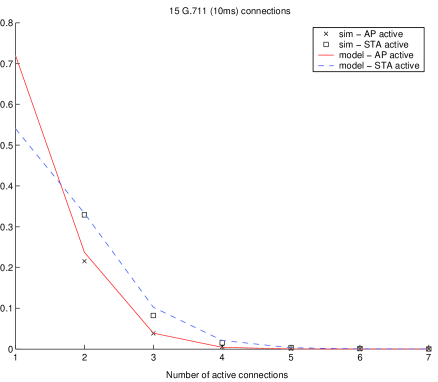
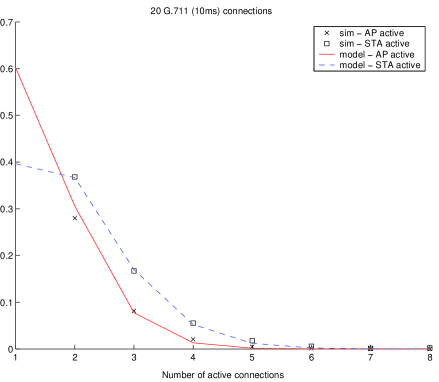
(a)	(b)
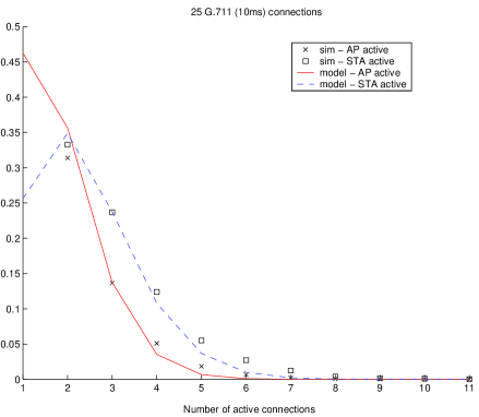
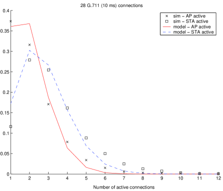
(c)	(d)

Figure 9: The pdf of active number of TCs given that the TC at the AP or at the station (denoted as STA) is active in a scenario consisting of G.711 VoIP connections (10 ms packet intervals). (a) 15 connections. (b) 20 connections. (c) 25 connections. (d) 28 connections. Note that the figures do not present the whole x-axis (activity profile for large number of stations) for better clarity on the comparison of simulation and analysis (especially when the activity probability is not close to zero).

Fig. 9 shows the probability density function (pdf) of active number of TCs given that the TC at the AP or at the non-AP station (denoted as STA in the figure) is active in a scenario consisting of only VoIP connections (G.711 VoIP codec with 10 ms packet intervals). As previously stated, we analytically calculate $P_{TC_{0},TC_{1},...,TC_{j},...,TC_{J-1}}^{j}(f^{\prime}_{0},f^{\prime}_{1},...,f^{\prime}_{j},...,f^{\prime}_{J-1})$ by assuming that the distribution of the number of active TCs approximates a Binomial distribution with parameters $f_{j}$ and $\rho_{j}$. The comparison in Fig. 9 shows that the pdf of analytical calculation closely follows the pdf obtained through simulation. Although the results are not presented here, a similar discussion holds for other codecs with different packet interval values. The pdf results for simulations are obtained through averaging over several simulation runs with different random number generator seeds and randomized flow start times.

V-D2 Voice Capacity Analysis in the Presence of Background Traffic

In the second set of experiments, we investigate the VoIP capacity when heavy background traffic coexists. Note that the analytical models of [29, 30, 31, 32, 33, 34, 35] do not provide such analysis capability. Table II shows the number of admitted G.711 VoIP flows for increasing the number of two-way background data connections. The comparison of analytical and simulation results shows that the proposed admission control scheme is highly accurate when a number of TCs (background) are always assumed active while some others (VoIP) are in nonsaturation. As the comparison of Tables I and II presents, the coexistence of background traffic is a big hit on the multimedia capacity of the WLAN. When the number of data connections is 5, the number of admitted flows decreases by around $30\%$. The decrease ratio goes up to $60\%$ when the number of data connections is increased to 30. Interestingly, the decrease ratio is almost insensitive to packet sampling interval length. Although the results are not presented, a similar discussion holds when VoIP flows employ G.729 codec.

V-D3 Voice and Video Capacity Analysis

In the third set of experiments, we investigate the capacity of 802.11e WLAN when both voice and video traffic coexist (using different ACs). Once again, note that the analytical models of [29, 30, 31, 32, 33, 34, 35] do not provide such analysis capability. Table III shows the number of admitted uplink, downlink, and two-way MPEG-4 flows for increasing the number of VoIP connections. In this scenario, we use the G.711 codec with a 20 ms sample interval. As the results indicate, the analytical and simulation results closely follow each other. Such a comparison reveals that the proposed capacity prediction and admission control scheme is also effective when different classes of multimedia traffic coexist in the BSS. As the comparison of the number of admitted uplink and downlink flows shows, channel contention overhead in the main limitation on capacity. For the same number of coexisting VoIP connections, the number of admitted downlink flows is larger than the number of admitted uplink flows, as contention overhead is much lower in the downlink scenario. With increasing number of VoIP connections, the difference increases as well. As expected, the two-way video capacity in terms of admitted number of flows is less than the capacity in the uplink only and the downlink only scenarios. The increasing VoIP load does not affect the ratio of downlink to two-way video capacity as significantly as it affects the ratio of the ratio of downlink to uplink video capacity.

VI Conclusion

We have developed a simple and novel average cycle time model to evaluate the performance of the EDCA function in saturation. The proposed model captures the performance in the case of an arbitrary assignment of AC-specific AIFS and CW values and is the first model to consider an arbitrary distribution of active ACs at the stations. We have shown that the analytical results obtained using the cycle time model closely follow the accurate predictions of the previously proposed more complex analytical models and simulation results. The proposed cycle time analysis can serve as a simple and practical alternative model for EDCA saturation throughput analysis.

We have also designed a practical and simple multimedia capacity prediction and admission control algorithm to limit the number of admitted realtime multimedia flows in the 802.11e infrastructure BSS. Motivated by the previous findings in the literature such that the contention-based 802.11 MAC can achieve high throughput and low delay in nonsaturation, the proposed admission control algorithm is based on simple tests on station- and AC-specific queue utilization ratio estimates. Our novel approach is the calculation of the queue utilization ratio by weighing the average service time predictions of the proposed cycle time saturation model among varying number of active stations. The proposed simple framework is effective in capacity estimation in the case of coexisting multimedia flows using different ACs with arbitrarily selected MAC parameters. Comparing the theoretical results with simulations, we have shown that the proposed algorithm provides guaranteed QoS for coexisting voice or video connections. One of the key insights provided by this study is the accuracy of the proposed approximate capacity estimation framework that uses relatively simpler saturation analysis rather than defining a more complex and hard to implement nonsaturation model.

TABLE I: Comparison of the Maximum Number of VoIP Connections

Sample Period	G.711		G.729
	Analysis/Simulation	[33]	Analysis/Simulation	[33]
10 ms	27/27	21	29/29	22
20 ms	49/49	38	56/56	43
30 ms	70/70	53	85/85	65
40 ms	87/87	67	112/112	85
50 ms	102/102	79	139/139	106
60 ms	115/115	89	166/166	128

TABLE II: Comparison of the Maximum Number of G.711 VoIP Connections (Analysis/Simulation) when heavy background traffic coexist.

VoIP Codec	Sample Period	Number of co-existing two-way background data connections
		5	10	15	20	25	30
G.711	10 ms	19/18	16/16	14/14	12/12	11/11	10/10
	20 ms	35/35	29/29	26/25	23/22	21/20	19/18
	30 ms	49/47	41/41	36/36	32/32	29/29	27/27
	40 ms	62/62	52/52	45/45	40/40	37/37	34/34
	50 ms	73/73	61/61	53/53	47/47	43/43	40/40
	60 ms	83/84	69/69	60/60	54/54	49/50	45/47

TABLE III: Comparison of the Maximum Number of Video Connections (Analysis/Simulation) when VoIP flows coexist.

		Number of existing two-way G.711 (20 ms) connections
		5	10	15	20	25	30
Number of admitted MPEG-4 flows	Downlink	109/110	98/100	87/88	76/78	64/65	52/54
	Uplink	88/89	67/69	57/57	48/48	37/37	28/28
	Two-way	54/55	46/47	41/41	34/34	28/28	19/19

References

- [1] IEEE Standard 802.11: Wireless LAN medium access control (MAC) and physical layer (PHY) specifications, IEEE 802.11 Std., 1999.
- [2] IEEE Standard 802.11: Wireless LAN medium access control (MAC) and physical layer (PHY) specifications: Medium access control (MAC) Quality of Service (QoS) Enhancements, IEEE 802.11e Std., 2005.
- [3] K. Medepalli and F. A. Tobagi, “Throughput Analysis of IEEE 802.11 Wireless LANs using an Average Cycle Time Approach,” in Proc. IEEE Globecom ’05, November 2005.
- [4] X. Chen, H. Zhai, X. Tian, and Y. Fang, “Supporting QoS in IEEE 802.11e Wireless LANs,” IEEE Trans. Wireless Commun., pp. 2217–2227, August 2006.
- [5] H. Zhai, X. Chen, and Y. Fang, “How Well Can the IEEE 802.11 Wireless LAN Support Quality of Service?” IEEE Trans. Wireless Commun., pp. 3084–3094, November 2005.
- [6] G. Bianchi, “Performance Analysis of the IEEE 802.11 Distributed Coordination Function,” IEEE Trans. Commun., pp. 535–547, March 2000.
- [7] F. Cali, M. Conti, and E. Gregori, “Dynamic Tuning of the IEEE 802.11 Protocol to Achieve a Theoretical Throughput Limit,” IEEE/ACM Trans. Netw., pp. 785–799, December 2000.
- [8] J. C. Tay and K. C. Chua, “A Capacity Analysis for the IEEE 802.11 MAC Protocol,” Wireless Netw., pp. 159–171, July 2001.
- [9] Y. Xiao, “Performance Analysis of Priority Schemes for IEEE 802.11 and IEEE 802.11e Wireless LANs,” IEEE Trans. Wireless Commun., pp. 1506–1515, July 2005.
- [10] Z. Kong, D. H. K. Tsang, B. Bensaou, and D. Gao, “Performance Analysis of the IEEE 802.11e Contention-Based Channel Access,” IEEE J. Select. Areas Commun., pp. 2095–2106, December 2004.
- [11] J. W. Robinson and T. S. Randhawa, “Saturation Throughput Analysis of IEEE 802.11e Enhanced Distributed Coordination Function,” IEEE J. Select. Areas Commun., pp. 917–928, June 2004.
- [12] J. Hui and M. Devetsikiotis, “A Unified Model for the Performance Analysis of IEEE 802.11e EDCA,” IEEE Trans. Commun., pp. 1498–1510, September 2005.
- [13] H. Zhu and I. Chlamtac, “Performance Analysis for IEEE 802.11e EDCF Service Differentiation,” IEEE Trans. Wireless Commun., pp. 1779–1788, July 2005.
- [14] I. Inan, F. Keceli, and E. Ayanoglu, “Saturation Throughput Analysis of the 802.11e Enhanced Distributed Channel Access Function,” in Proc. IEEE ICC ’07, June 2007.
- [15] Z. Tao and S. Panwar, “Throughput and Delay Analysis for the IEEE 802.11e Enhanced Distributed Channel Access,” IEEE Trans. Commun., pp. 596–602, April 2006.
- [16] J. Zhao, Z. Guo, Q. Zhang, and W. Zhu, “Performance Study of MAC for Service Differentiation in IEEE 802.11,” in Proc. IEEE Globecom ’02, November 2002.
- [17] A. Banchs and L. Vollero, “Throughput Analysis and Optimal Configuration of IEEE 802.11e EDCA,” Comp. Netw., pp. 1749–1768, August 2006.
- [18] Y. Lin and V. W. Wong, “Saturation Throughput of IEEE 802.11e EDCA Based on Mean Value Analysis,” in Proc. IEEE WCNC ’06, April 2006.
- [19] Y.-L. Kuo, C.-H. Lu, E. H.-K. Wu, G.-H. Chen, and Y.-H. Tseng, “Performance Analysis of the Enhanced Distributed Coordination Function in the IEEE 802.11e,” in Proc. IEEE VTC ’03 - Fall, October 2003.
- [20] K. Duffy, D. Malone, and D. J. Leith, “Modeling the 802.11 Distributed Coordination Function in Non-Saturated Conditions,” IEEE Commun. Lett., pp. 715–717, August 2005.
- [21] F. Alizadeh-Shabdiz and S. Subramaniam, “Analytical Models for Single-Hop and Multi-Hop Ad Hoc Networks,” Mobile Networks and Applications, pp. 75–90, February 2006.
- [22] G. R. Cantieni, Q. Ni, C. Barakat, and T. Turletti, “Performance Analysis under Finite Load and Improvements for Multirate 802.11,” Comp. Commun., pp. 1095–1109, June 2005.
- [23] P. E. Engelstad and O. N. Osterbo, “Analysis of the Total Delay of IEEE 802.11e EDCA and 802.11 DCF,” in Proc. IEEE ICC ’06, June 2006.
- [24] O. Tickoo and B. Sikdar, “A Queueing Model for Finite Load IEEE 802.11 Random Access MAC,” in Proc. IEEE ICC ’04, June 2004.
- [25] H. Zhai, Y. Kwon, and Y. Fang, “Performance Analysis of IEEE 802.11 MAC Protocols in Wireless LANs,” Wireless Communications and Mobile Computing, pp. 917–931, December 2004.
- [26] C. H. Foh and M. Zukerman, “A New Technique for Performance Evaluation of Random Access Protocols,” in Proc. European Wireless ’02, February 2002.
- [27] J. W. Tantra, C. H. Foh, I. Tinnirello, and G. Bianchi, “Analysis of the IEEE 802.11e EDCA Under Statistical Traffic,” in Proc. IEEE ICC ’06, June 2006.
- [28] J. Hui and M. Devetsikiotis, “Metamodeling of Wi-Fi Performance,” in Proc. IEEE ICC ’06, June 2006.
- [29] K. Medepalli and F. A. Tobagi, “System Centric and User Centric Queueing Models for IEEE 802.11 based Wireless LANs,” in Proc. IEEE Broadnets ’05, October 2005.
- [30] D. P. Hole and F. A. Tobagi, “Capacity of an IEEE 802.11b Wireless LAN Supporting VoIP,” in Proc. IEEE ICC ’04, June 2004.
- [31] S. Garg and M. Kappes, “An Experimental Study of Throughput for UDP and VoIP Traffic in IEEE 802.11b Networks,” in Proc. IEEE WCNC ’03, March 2003.
- [32] ——, “Can I Add a VoIP Call?” in Proc. IEEE ICC ’03, May 2003.
- [33] L. X. Cai, X. Shen, J. W. Mark, L. Cai, and Y. Xiao, “Voice Capacity Analysis of WLAN with Unbalanced Traffic,” IEEE Trans. Veh. Technol., pp. 752–761, May 2006.
- [34] D. Gao, J. Cai, and C. W. Chen, “Capacity Analysis of Supporting VoIP in IEEE 802.11e EDCA WLANs,” in Proc. IEEE Globecom ’06, November 2006.
- [35] Y. Cheng, L. Cai, X. Ling, W. Song, W. Zhuang, X. Shen, and A. Leon-Garcia, “Improvement of WLAN QoS Capability via Statistical Multiplexing,” in Proc. IEEE Globecom ’06, November 2006.
- [36] L. Zhang and S. Zeadally, “HARMONICA: Enhanced QoS Support with Admission Control for IEEE 802.11 Contention-based Access,” in Proc. IEEE RTAS ’04, May 2004.
- [37] D. Pong and T. Moors, “Call Admission Control for IEEE 802.11 Contention Access Mechanism,” in Proc. IEEE Globecom ’03, December 2003.
- [38] J. He, D. Kaleshi, A. Munro, M. Barton, Z. Tang, and Z. Yang, “Management of Services Differentiation and Guarantee in IEEE 802.11e Wireless LANs,” in Proc. IEEE VTC ’05 - Spring, May 2005.
- [39] Y. Xiao and H. Li, “Voice and Video Transmissions with Global Data Parameter Control for the IEEE 802.11e Enhanced Distributed Channel Access,” IEEE Trans. Parallel Distrib. Syst., pp. 1041–1053, November 2004.
- [40] ——, “Local Data Control and Admission Control for QoS Support in Wireless Ad Hoc Networks,” IEEE Trans. Veh. Technol., pp. 1558–1572, September 2004.
- [41] Y. Xiao and Y. Pan, “Differentiation, QoS Guarantee, and Optimization for Real-Time Traffic over One-Hop Ad Hoc Networks,” IEEE Trans. Parallel Distrib. Syst., pp. 538–549, June 2005.
- [42] Y. Xiao, “QoS Guarantee and Provisioning at the Contention-Based Wireless MAC Layer in the IEEE 802.11e Wireless LANs,” IEEE Wireless Commun. Mag., pp. 14–21, February 2006.
- [43] (2006) The Network Simulator, ns-2. [Online]. Available: http://www.isi.edu/nsnam/ns
- [44] IEEE 802.11e HCF MAC model for ns-2.28. [Online]. Available: http://newport.eecs.uci.edu/fkeceli/ns.htm
- [45] IEEE Standard 802.11: Wireless LAN medium access control (MAC) and physical layer (PHY) specifications: Further Higher Data Rate Extension in the 2.4 GHz Band, IEEE 802.11g Std., 2003.
- [46] P. Serrano, A. Banchs, T. Melia, and L. Vollero, “Performance Anomalies of nonoptimally configured Wireless LANs,” in Proc. IEEE WCNC ’06, April 2006.
- [47] P. Seeling, M. Reisslein, and B. Kulapala, “Network Performance Evaluation Using Frame Size and Quality Traces of Single-Layer and Two-Layer Video: A Tutorial,” IEEE Communications Surveys and Tutorials, vol. 6, no. 2, pp. 58–78, Third Quarter 2004. [Online]. Available: http://www.eas.asu.edu/trace