Proceedings of the $11$th World Congress in Mechanism and Machine Science
August $18$-$21$, $2003$, Tianjin, China
China Machinery Press, edited by Tian Huang
A Comparative Study between Two Three-DOF Parallel Kinematic Machines using Kinetostatic Criteria and Interval Analysis
Damien Chablat¹ Philippe Wenger¹ Jean-Pierre Merlet ^2
1Institut de Recherche en Communications et Cybernétique de Nantes
1, rue de la Noë, 44321 Nantes, France,
²INRIA Sophia-Antipolis, 2004 Route des Lucioles,
06902 Sophia Antipolis, France,
Damien.Chablat@irccyn.ec-nantes.fr and Jean-Pierre.Merlet@sophia.inria.fr

Abstract: This paper addresses the workspace analysis of two 3-DOF translational parallel mechanisms designed for machining applications. The two machines features three fixed linear joints. The joint axes of the first machine are orthogonal whereas these of the second are parallel. In both cases, the mobile platform moves in the Cartesian $x-y-z$ space with fixed orientation. The workspace analysis is conducted on the basis of prescribed kinetostatic performances. Interval analysis based methods are used to compute the dextrous workspace and the largest cube enclosed in this workspace.

Keywords: Parallel kinematic architecture, Singularity, Workspace, Transmissions factors, Stiffness, Design, Interval analysis.

${\bf 1}$ Introduction

Parallel kinematic machines (PKM) are known for their high dynamic performances and low positioning errors. The kinematic design of PKM has drawn the interest of several researchers. The workspace is usually considered as a relevant design criterion [1, 2, 3]. Parallel singularities [4] occur in the workspace where stiffness is lost, and thus are very undesirable. They are generally eliminated by design. The Jacobian matrix, which relates the joint rates to the output velocities is generally not constant and not isotropic. Consequently, the performances (e.g. maximum speeds, forces, accuracy and stiffness) vary considerably for different points in the Cartesian workspace and for different directions at one given point. This is a serious drawback for machining applications [5, 6, 7]. Some parallel mechanisms were recently shown to be isotropic throughout the workspace [8, 9, 10]. But their legs are subject to bending which is not desirable for machining applications . To be of interest for machining applications, a PKM should preserve good workspace properties, that is, regular shape and acceptable kinetostatic performances throughout. In milling applications, the machining conditions must remain constant along the whole tool path [11, 12]. In many research papers, this criterion is not taken into account in the algorithmic methods used to calculate the workspace volume [13, 14].

This paper compares two PKM with three translational DOF derived from the Delta robot originally designed by Reymond Clavel for pick-and-place operations [2]. The first one, called UraneSX (Renault Automation) [15], has three non coplanar horizontal linear joints, like the Quickstep (Krause & Mauser) . The second one, called Orthoglide, has three orthogonal linear joints [16].

The comparative study is conducted on the basis of the size of a prescribed workspace with bounded velocity and force transmission factors, called the dextrous workspace. Interval analysis based method is used to compute the dextrous workspace as well as the largest cube enclosed in this workspace [21].

Next section presents the Orthoglide and UraneSX mechanisms. The kinematic equations and the singularity analysis are detailed in Section 3. Section 4 is devoted to the determination of the largest cube enclosed in the dextrous workspace and to the comparative study between the two mechanisms.

${\bf 2}$ Description of the Orthoglide and the UraneSX

Most existing PKM can be classified into two main families. PKM of the first family have fixed foot points and variable length struts and are generally called “hexapods”. PKM of the second family have variable foot points and fixed length struts. They are interesting because the actuators are fixed and thus the moving masses are lower than in the hexapods and tripods.

The Orthoglide and the UraneSX mechanisms studied in this paper are $3$-axis translational PKM and belong to the second family. Figures 1 and 2 show the general kinematic architecture of the Orthoglide and of the UraneSX, respectively. Both mechanisms have three parallel $PRPaR$ identical chains (where $P$, $R$ and $Pa$ stand for Prismatic, Revolute and Parallelogram joint, respectively). The actuated joints are the three linear joints.

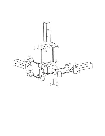
Figure 1: Orthoglide kinematic architecture

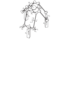
Figure 2: UraneSX kinematic architecture

The output body is connected to the linear joints through a set of three parallelograms of equal lengths $L~{}=~{}A_{i}B_{i}$, so that it can move only in translation. Vectors ${\bf{e}}_{i}$ coincide with the direction of the $i$th linear joint. The base points $A_{i}$ are located at the middle of the first two revolute joints of the $i^{th}$ parallelogram, and $B_{i}$ is at the middle of the last two revolute joints of the $i^{th}$ parallelogram.

For the Orthoglide mechanism, the first linear joint axis is parallel to the $x$-axis, the second one is parallel to the $y$-axis and the third one is parallel to the $z$-axis. When each vector ${\bf{e}}_{i}$ is aligned with ${\bf{A}}_{i}{\bf{B}}_{i}$, the Orthoglide is in an isotropic configuration and the tool center point $P$ is located at the intersection of the three linear joint axes.

The linear joint axes of the UraneSX mechanism are parallel to the $z$-axis. In fig. 2, points $A_{1}$, $A_{2}$ and $A_{3}$ are the vertices of an equilateral triangle whose geometric center is $O$ and such that $OA_{i}=R$. Thus, points $B_{1}$, $B_{2}$ and $B_{3}$ are the vertices of an equilateral triangle whose geometric center is $P$, and such that $OB_{i}=r$.

${\bf 3}$ Kinematic Equations and Singularity Analysis

We recall briefly here the kinematics and the singularities of the Orthoglide and of the UraneSX (See [15, 16] for more details).

${\bf 3.1}$ Kinematic equation and singularity analysis

Let $\theta_{i}$ and $\beta_{i}$ denote the joint angles of the parallelogram about axes ${\bf{i}}_{i}$ and ${\bf{j}}_{i}$, respectively (Figs. 1 and 2). Let ${\bf{\rho}}_{1}$, ${\bf{\rho}}_{2}$, ${\bf{\rho}}_{3}$ denote the linear joint variables and $L$ denote the length of the three legs, $A_{i}B_{i}$.

For the Orthoglide, the position vector p of the tool center point $P$ is defined in a reference frame (O, $x$, $y$, $z$) centered at the intersection of the three linear joint axes (note that the reference frame has been translated in Fig. 1 for more legibility).

For the UraneSX, the position vector p of the tool center point $P$ is defined in a reference frame (O, $x$, $y$, $z$) centered at the geometric center of the points $A_{1}$, $A_{2}$, and $A_{3}$ (same remark as above).

Let $\dot{\mbox{\boldmath${\rho}$\unboldmath}}$ be referred to as the vector of actuated joint rates and $\dot{{\bf{p}}}$ as the velocity vector of point $P$:

$$\dot{\mbox{\boldmath${\rho}$\unboldmath}}=[\dot{\rho}_{1}~{}\dot{\rho}_{2}~{}\dot{\rho}_{3}]^{T},\quad\dot{{\bf{p}}}=[\dot{x}~{}\dot{y}~{}\dot{z}]^{T}$$

$\dot{{\bf{p}}}$ can be written in three different ways by traversing the three chains $A_{i}B_{i}P$:

$$\dot{{\bf{p}}}={\bf{e}}_{i}\dot{\rho}_{i}+(\dot{\theta}_{i}{\bf{i}}_{i}+\dot{\beta}_{i}{\bf{j}}_{i})\times({\bf{b}}_{i}-{\bf{a}}_{i})\\$$ (1)

where ${\bf{b}}_{i}$ and ${\bf{c}}_{i}$ are the position vectors of the points $B_{i}$ and $C_{i}$, respectively, and ${\bf{e}}_{i}$ is the direction vector of the linear joints, for $i=1,2,$3.

We want to eliminate the three idle joint rates $\dot{\theta}_{i}$ and $\dot{\beta}_{i}$ from Eqs. (1), which we do by dot-multiplying Eqs. (1) by ${\bf{b}}_{i}-{\bf{a}}_{i}$:

$$({\bf{b}}_{i}-{\bf{a}}_{i})^{T}\dot{{\bf{p}}}=({\bf{b}}_{i}-{\bf{a}}_{i})^{T}{\bf{e}}_{i}\dot{\rho}_{i}$$ (2)

Equations (2) can now be cast in vector form, namely ${\bf{A}}\dot{\bf p}={\bf{B}}\dot{\mbox{\boldmath${\rho}$\unboldmath}}$, where A and B are the parallel and serial Jacobian matrices, respectively:

$${\bf{A}}=\left[\begin{array}[]{c}({\bf{b}}_{1}-{\bf{a}}_{1})^{T}\\ ({\bf{b}}_{2}-{\bf{a}}_{2})^{T}\\ ({\bf{b}}_{3}-{\bf{a}}_{3})^{T}\end{array}\right]{\rm~{}~{}and~{}~{}}{\bf{B}}=\left[\begin{array}[]{ccc}\eta_{1}&0&0\\ 0&\eta_{2}&0\\ 0&0&\eta_{3}\end{array}\right]$$ (9)

with $\eta_{i}=({\bf{b}}_{i}-{\bf{a}}_{i})^{T}{\bf{e}}_{i}$ for $i=1,2,3$.

Parallel singularities occur when the determinant of the matrix A vanishes, i.e. when $\det({\bf{A}})=0$. Eq. (9) shows that the parallel singularities occur when:

$$({\bf{b}}_{1}-{\bf{a}}_{1})=\alpha({\bf{b}}_{2}-{\bf{a}}_{2})+\lambda({\bf{b}}_{3}-{\bf{a}}_{3})$$

that is when the points $A_{1}$, $B_{1}$, $A_{2}$, $B_{2}$, $A_{3}$ and $B_{3}$ lie in parallel planes. A particular case occurs when the links $A_{i}B_{i}$ are parallel:

$$({\bf{b}}_{1}-{\bf{a}}_{1})//({\bf{b}}_{2}-{\bf{a}}_{2})\quad{\rm and}\quad({\bf{b}}_{2}-{\bf{a}}_{2})//({\bf{b}}_{3}-{\bf{a}}_{3})$$ (10)

$$\quad{\rm and}\quad({\bf{b}}_{3}-{\bf{a}}_{3})//({\bf{b}}_{1}-{\bf{a}}_{1})$$

Serial singularities arise when the serial Jacobian matrix B is no longer invertible i.e. when $\det({\bf{B}})=0$. At a serial singularity a direction exists along which no Cartesian velocity can be produced. Equation (9) shows that $\det({\bf{B}})=0$ when for one leg $i$, $({\bf{b}}_{i}-{\bf{a}}_{i})\perp({\bf{b}}_{i}-{\bf{a}}_{i})$.

When A is not singular, we can write,

$$\dot{{\bf{p}}}={\bf{J}}\dot{\mbox{\boldmath${\rho}$\unboldmath}}{\rm~{}with~{}}{\bf{J}}={\bf{A}}^{-1}{\bf{B}}$$ (11)

${\bf 3.2}$ Velocity transmission factors

For joint rates belonging to a unit ball, namely, $||\dot{\mbox{\boldmath${\rho}$\unboldmath}}||\leq 1$, the Cartesian velocities belong to an ellipsoid such that:

$$\dot{\mbox{\boldmath${p}$\unboldmath}}^{T}({\bf{J}}{\bf{J}}^{T})\dot{\mbox{\boldmath${p}$\unboldmath}}\leq 1$$

The eigenvectors of matrix ${\bf{J}}{\bf{J}}^{T}$ define the direction of the principal axes of this ellipsoid. The square roots $\psi_{1}$, $\psi_{2}$ and $\psi_{3}$ of the real eigenvalues $\sigma_{1}$, $\sigma_{2}$ and $\sigma_{3}$ of ${\bf{J}}{\bf{J}}^{T}$, i.e. the lengths of the aforementioned principal axes are the velocity transmission factors in the principal axes directions. To limit the variations of these factors in the Cartesian workspace, we set

$$\psi_{min}\leq\psi_{i}\leq\psi_{max}$$ (12)

throughout the workspace. To simplify the problem, we set $\psi_{min}=1/\psi_{max}$ where the value of $\psi_{max}$ depends on given performance requirements.

${\bf 4}$ Determination of the largest cube enclosed in the dextrous workspace

For usual machine tools, the Cartesian workspace shape is generally a parallelepiped. Due to the symmetrical architecture of the Orthoglide, the Cartesian workspace has a fairly regular shape in which it is possible to include a cube whose sides are parallel to the planes $xy$, $yz$ and $xz$ respectively.

The Cartesian workspace of the UraneSX is the intersection of three cylinders whose axes are parallel to the $z$-axis. Thus, the workspace is theoretically unlimited in the $z$-direction and the Jacobian matrix does not depend on the $z$ coordinate. Practically, only the limits on the linear joints define the limits of the Cartesian workspace in the $z$-directions.

The aim of the following section is to define the edge length of the largest cube enclosed in the dextrous workspace of the Orthoglide and the edge length of the largest square enclosed in the dextrous workspace of the UraneSX, as well as the location of their respective centers for both mechanisms. This is done using an interval analysis method. Unlike numerical computing methods, such a method allows to prove formally that the velocity amplification factors lie in the predefined range $[\psi_{min}~{}\psi_{max}]$ in a given subpart of the Cartesian workspace.

Two algorithms are described to define (i) a set of boxes in the Cartesian workspace in which the velocity amplification factors remain under the prescribed values, and (ii) the largest cube enclosed in the dextrous workspace.

${\bf 4.1}$ Box verification

A basic tool of the algorithm is a module ${\cal M}(B)$ that takes as input a Cartesian box $B$ and whose output is:

• either that for any point in the box the eigenvalues lie in the range $[\sigma_{min},\sigma_{max}]$

• or that for any point in the box one of the eigenvalues is either lower than $\sigma_{min}$ or larger than $\sigma_{max}$

• or that the two previous conditions does not hold for all the points of the box i.e. that for some points the eigenvalues lie in the range $[\sigma_{min},\sigma_{max}]$ while this is not true for some other points

The first step of this module consists in considering an arbitrary point of the box (e.g. its center) and to compute the eigenvalues at this point: either all of them lie in the range $[\sigma_{min},\sigma_{max}]$ or at least one of them lie outside this range.

In the first case if we are able to check that there is no point in $B$ such that one of the eigenvalues at this point is be equal to $\sigma_{min}$ or $\sigma_{max}$, then we can guarantee that for any point in $B$ the eigenvalues will be in the range $[\sigma_{min},\sigma_{max}]$. Indeed assume that at a given point $B$ the lowest eigenvalue is lower than $\sigma_{min}$: this implies that somewhere along the line joining this point to the center of the box the lowest eigenvalue will be exactly $\sigma_{min}$. To perform this check we substitute $\sigma_{min}$ to the unknown in the characteristic polynomial of ${\bf{J}}{\bf{J}}^{T}$ to get a polynomial in $x,y,z$ only. We now have to check if there exists some values for these three cartesian coordinates that cancel the polynomial, being understood that these values have to define a point belonging to $B$: this is done by using an interval analysis algorithm from the ALIAS library [21].

Assume now that at the center of the box the largest eigenvalue is greater than $\sigma_{max}$. If there is no point in $B$ such that one of the eigenvalues is equal to $\sigma_{max}$, then we can guarantee that for any point in $B$ the largest eigenvalue will always be greater than $\sigma_{max}$. This check is performed by using the same method as in the previous case. Hence the ${\cal M}$ module will return:

• 1: if for all points in $B$ the eigenvalues lie in $[\sigma_{min},\sigma_{max}]$ (hence $B$ is in the dextrous workspace)

• -1: if for all points in $B$ either the largest eigenvalue is always greater than $\sigma_{max}$ or the lowest eigenvalue is lower than $\sigma_{min}$ (hence $B$ is outside the dextrous workspace).

• 0: in the other cases i.e. parts of $B$ may be either outside or inside the dextrous workspace

${\bf 4.2}$ Determination of the dextrous workspace

The dextrous workspace ${\cal W}$ is here defined as the loci of the points for which square real roots of the eigenvalues of the matrix ${\bf{J}}{\bf{J}}^{T}$, i.e. the velocity transmission factors, lie within the predefined range $[\sigma_{min},\sigma_{max}]$. The eigenvalues are determined by solving the third degree characteristic polynomial of the matrix ${\bf{J}}{\bf{J}}^{T}$.

The polynomial is only defined for the points within the intersection ${\cal I}$ of the three cylinders defined by

$$x^{2}+y^{2}\leq L\quad x^{2}+z^{2}\leq L\quad y^{2}+z^{2}\leq L$$

for the Orthoglide, and,

$$(x-R+r)^{2}+y^{2} \leq L$$

$$\left(x-(R-r)/2\right)^{2}+\left(y-(R-r)\sqrt{3}/2\right)^{2} \leq L$$

$$\left(x-(R-r)/2\right)^{2}+\left(y+(R-r)\sqrt{3}/2\right)^{2} \leq L$$

for the UraneSX.

To solve numerically the above equations and to compare the two mechanisms, the length of the legs is normalized, i.e. we set $L=1$.

${\bf 4.3}$ Algorithm

We will now describe a method for determining a cube that is enclosed in the workspace of both mechanisms, whose edge length is $2W$ and such that there is no other cube enclosed in the workspace with an edge length of $2(W+\alpha)$, where $\alpha$ is an accuracy threshold fixed in advance.

The first step is to determine the largest cube enclosed in the workspace with a center located at (0,0,0). This is done by using the ${\cal M}$ module on the Cartesian box $B_{init}$ $[-k\alpha,k\alpha],[-k\alpha,k\alpha],[-k\alpha,k\alpha]$ where $k$ is an integer initialized to 1. Each time the ${\cal M}$ module returns 1 for $B_{init}$ (which means that the cube with edge length $2k\alpha$ is enclosed in the dextrous workspace) we double the value of $k$. If this module returns -1 for a value of $k$ larger than 1 this implies that the cube with edge length $k\alpha/2$ lie in the dextrous workspace while the cube with edge length $k\alpha$ does not. Hence we restart the process with $k=k/2+1$.Otherwise we have determined that the cube with edge length $2k\alpha$ is enclosed in the dextrous workspace, while the cube with edge length $2(k+1)\alpha$ does not. The value $2k\alpha$ is hence an initial value for $W$.

We then use the following algorithm for determining the largest cube enclosed in the dextrous workspace. We start with the Cartesian box $B_{0}$= $[-L,L]$, $[-L,L]$, $[-L,L]$ that enclose the workspace and we use a list of Cartesian boxes ${\cal L}$ indexed by $i$ with $n$ elements:

1. If $i>n$ EXIT

2. Using interval arithmetics, check if $B_{i}$ contains points such that a box centered at these points with edge length $W+\alpha$ is fully enclosed in the workspace.

   1. If the box does not contain such points discard the box, set $i$ to $i+1$ and restart.

   2. If the box contains points that belong and point that does not belong to the workspace, check if the box has at least one range that is larger than $\alpha$. If not, there is no point in the box that can be the center of a cube with edge length at least $W+\alpha$ and that is enclosed in the workspace. Hence we may discard this box. If yes bissect the box along one of this range, thereby creating 2 new boxes that are stored at the end of ${\cal L}$. Set $i$ to $i+1$ and restart.

3. At this stage the box $B_{i}$ contains only points that may be the center of a cube with edge length at least $W+\alpha$ and fully enclosed in the workspace.

4. If the maximal width of the box is lower or equal to $\alpha$, use the procedure described for the center at (0,0,0) to determine the largest cube centered at the center of the box that lie within the dextrous workspace. If this procedure provides a cube with edge length larger than $W$, update $W$. Set $i$ to $i+1$ and restart.

5. If the maximal width of the box is greater than $\alpha$ use the procedure described for the center at (0,0,0) to determine the largest cube centered at the center of the box that lie within the dextrous workspace. If this procedure provides a cube with edge length larger than $W$, update $W$. Select a variable of the box that has a range larger than $\alpha$, bissect the box, thereby creating 2 new boxes that are stored at the end of ${\cal L}$. Set $i$ to $i+1$ and restart.

This procedure ensures to determine a cube with edge length $W$ that is enclosed in the workspace and in the dextrous workspace, while there is no such cube with edge length $W+\alpha$.

${\bf 4.4}$ Design parameters and results

To compare the two mechanisms, the leg length $L$ is set to 1 and the bounds on the velocity factor amplification are $\psi=[0.5~{}2]$ with $\alpha=0.001$. For the UraneSX, it is necessary to define two additional lengths, $r$ and $R$. However, the edge length of the workspace only depends on $R-r$.

For the Orthoglide, we found out that the largest cube has its center located at $(0.086,0.086,0.086)$ and that its edge length is $L_{Workspace}=0.644$.

For the UraneSX, the design parameters are those defined in [15], which we have normalized to have $L=1$, i.e. $r=3/26$ and $R=7/13$. To compare the two mechanisms, we increase the value of $R$ such that $R^{\prime}=R+\lambda$ with $\lambda=[0.0,0.2]$. For $R<7/13$, the constraints on the velocity amplification factors are not satisfied.

$\lambda$	Center	$L_{Workspace}$
0.00	(-0.0178,-0.0045)	0.510
0.05	(-0.0179,-0.0022)	0.470
0.10	(-0.0225,-0.0031)	0.420
0.15	(-0.0245,-0.0018)	0.370
0.20	(-0.0211,-0.0033)	0.320

Table 1: Variations of the edge length of the square workspace for the UraneSX mechanism

The optimal value of $R^{\prime}$ is obtained for $\lambda=0$, i.e. for the design parameters defined in [15] for an industrial application. To expand this square workspace in the $z$-direction, the range limits must be equal to the edge length of the square plus the range variations necessary to move throughout the square in the $x-y$ plane.

The constraints on the velocity amplification factors used for the design of the Orthoglide are close to those used for the design of the UraneSX, which is an industrial machine tool. For the same length of the legs, the size of the cubic workspace is larger for the Orthoglide than for the UraneSX.

For the Orthoglide, the optimization puts the serial and parallel singularities far away from the Cartesian workspace [16]. The UraneSX has no parallel singularities due to the design parameters ($R-r<L$), but serial singularity cannot be avoided with the previous optimization function. To produce the motion in the $z$-direction, the range limits of the linear joints are set such that the constraints on the velocity amplification factors are not satisfied throughout the Cartesian workspace.

${\bf 5}$ Conclusions

Two 3-DOf translational PKM are compared in this paper: the Orthoglide and the UraneSX. The dextrous workspace is defined as the part of the Cartesian workspace where the velocity amplification factors remain within a predefined range. The dextrous workspace is really available for milling tool paths because the performances are homogeneous in it. The largest cube for the Orthoglide and the largest square for the UraneSX enclosed in the dextrous workspace are computed using an interval analysis based method. This method is interesting because it allows to prove formally whether in a subpart of the Cartesian workspace the velocity amplification factors remain within a predefined range or not. These results can be used to design partially these mechanisms for milling applications.

References

- [1] Merlet, J-P., 1996, “Workspace-0riented Methodology for Designing a Parallel Manipulator,” IEEE Int. Conf. on Robotics and Automation, pp. 3726-3731.
- [2] Clavel, R., 1988, “DELTA, a Fast Robot with Parallel Geometry,” Proc. of the 18th Int. Symposium of Industrial Robots, IFR Publications, pp. 91-100.
- [3] Gosselin, C and Angeles, J., 1991, “A Global Performance Index for the Kinematic Optimization of Robotic Manipulators,” Journal of Mechanical Design, vol. 113, pp. 220-226.
- [4] Wenger, Ph. and Chablat, D., 1997, “Definition Sets for the Direct Kinematics of Parallel Manipulators,” 8th Int. Conf. Advanced Robotics, pp. 859-864.
- [5] Kim, J. Park, C. Kim, J. and Park, F.C. 1997, “Performance Analysis of Parallel Manipulator Architectures for CNC Machining Applications,” Proc. IMECE Symp. On Machine Tools, Dallas.
- [6] Treib, T. and Zirn, O. “Similarity laws of serial and parallel manipulators for machine tools,” Proc. Int. Seminar on Improving Machine Tool Performance, pp. 125–131, Vol. 1, 1998.
- [7] Wenger, P. Gosselin, C. and Chablat. D. 2001, “A Comparative Study of Parallel Kinematic Architectures for Machining Applications,” Proc. Workshop on Computational Kinematics’2001, Seoul, Korea, pp. 249–258.
- [8] Kong, X. and Gosselin, C. M., 2002, “A Class of 3-DOF Translational Parallel Manipulators with Linear I-O Equations,” Proc. of Workshop on Fundamental Issues and Future Research Directions for Parallel Mechanisms and Manipulators, Qu bec, Canada.
- [9] Carricato, M. and Parenti-Castelli, V., 2002, “Singularity-Free Fully-Isotropic Translational Parallel Mechanisms,” The International Journal of Robotics Research, Vol. 21, No. 2, pp. 161-174, February.
- [10] Kim, H.S. and Tsai, L.W., 2002, “Evaluation of a Cartesian manipulator,” in Lenarčič, J. and Thomas, F. (editors), Advances in Robot Kinematic, Kluwer Academic Publishers, June, pp. 21–38.
- [11] Rehsteiner, F., Neugebauer, R.. Spiewak, S. and Wieland, F., 1999, “Putting Parallel Kinematics Machines (PKM) to Productive Work,” Annals of the CIRP, Vol. 48:1, pp. 345–350.
- [12] Tlusty, J., Ziegert, J, and Ridgeway, S., 1999, “Fundamental Comparison of the Use of Serial and Parallel Kinematics for Machine Tools,” Annals of the CIRP, Vol. 48:1, pp. 351–356.
- [13] Luh C-M., Adkins F. A., Haug E. J. and Qui C. C., 1996, “Working Capability Analysis of Stewart platforms,” Trans. of ASME, pp. 220–227.
- [14] Merlet J-P., 1999, “Determination of 6D Workspace of Gough-Type Parallel Manipulator and Comparison between Different Geometries,” The Int. Journal of Robotic Research, Vol. 19, No. 9, pp. 902–916.
- [15] Company, O. Pierrot, F., 2002, “Modelling and Design Issues of a 3-axis Parallel Machine-Tool,” Mechanism and Machine Theory, Vol. 37, pp. 1325–1345.
- [16] Chablat, D. and Wenger, Ph, 2002, “Architecture Optimization of a 3-DOF Parallel Mechanism for Machining Applications, the Orthoglide,” IEEE Trans. Robotics and Automation, June, 2003.
- [17] Golub, G. H. and Van Loan, C. F., 1989, “Matrix Computations,” The John Hopkins University Press, Baltimore.
- [18] Salisbury J-K. and Craig J-J., 1982, “Articulated Hands: Force Control and Kinematic Issues,” The Int. J. Robotics Res., Vol. 1, No. 1, pp. 4–17.
- [19] Angeles J., 2002, “Fundamentals of Robotic Mechanical Systems,” Second Edition, Springer-Verlag, New York.
- [20] Yoshikawa, T., 1985, “Manipulability of Robot Mechanisms,” The Int. J. Robotics Res., Vol. 4, No. 2, pp. 3–9.
- [21] Merlet J-P., 2000, “ALIAS: an interval analysis based library for solving and analyzing system of equations,” SEA, June. Automation, pp. 1964–1969.