Very high energy observations of the BL Lac objects
3C 66A and OJ 287

Abstract

Abstract

Using the Solar Tower Atmospheric Cherenkov Effect Experiment (STACEE), we have observed the BL Lac objects 3C 66A and OJ 287. These are members of the class of low-frequency-peaked BL Lac objects (LBLs) and are two of the three LBLs predicted by Costamante and Ghisellini [1] to be potential sources of very high energy ($>$ 100 GeV) gamma-ray emission. The third candidate, BL Lacertae, has recently been detected by the MAGIC collaboration [2]. Our observations have not produced detections; we calculate a 99% CL upper limit of flux from 3C 66A of 0.15 Crab flux units and from OJ 287 our limit is 0.52 Crab. These limits assume a Crab-like energy spectrum with an effective energy threshold of 185 GeV.

1 Introduction

The field of very high energy (VHE) gamma-ray astronomy is a relatively young discipline that is concerned with the study of astrophysical sources of gamma rays with energies above 100 GeV. At these energies, all gamma-ray detections are indirect; they are made using ground-based telescopes which measure components of the air showers caused by the gamma rays. The lowest energy thresholds are achieved by telescopes which measure the Cherenkov light produced by particles in the showers. Detectors which record the arrival of the air shower particles themselves achieve wider fields of view and larger duty factors but operate at higher thresholds. The first reliable detection of an astrophysical source using the atmospheric Cherenkov technique was that of the Crab Nebula, made in the late 1980’s, by the Whipple collaboration [3]. Since then there has been rapid progress in the field (for a recent review see [4]).

The first extra-galactic VHE source to be detected was the blazar Markarian 421 [5]. Since its detection in 1992, more than a dozen other blazars have been detected at TeV energies and they constitute almost all of the known extra-galactic VHE sources. At lower (GeV) energies, 66 of the 271 sources in the EGRET catalog [6] have been identified as belonging to the blazar class, again constituting the majority of the identified extra-galactic sources.

Blazars are members of a class of Active Galactic Nuclei (AGNs). Simply described, an AGN is believed to comprise a super-massive ($10^{7}-10^{9}~{}M_{\bigodot}$) black hole surrounded by an accretion disk at the centre of a host galaxy. Relativistic jets emerge along the spin axis of the AGN. Blazars are those AGNs which have one of their jets pointed towards the Earth.

In the leading blazar paradigm, VHE gamma rays are produced by inverse-Compton (IC) scattering of low energy photons by a population of high energy electrons which have been shock-accelerated in the jet. These electrons, moving in the local magnetic fields, also produce synchrotron radiation. This scenario leads naturally to a double-hump spectral energy distribution (SED) with a low energy synchrotron peak and a higher energy IC peak. Blazars are often classified by the location of the synchrotron peak. Low-frequency-peaked blazars (LBLs) have this peak in the radio or optical band while for high-frequency-peaked blazars (HBLs), it is in the X-ray band. Costamante and Ghisellini [1] have studied a large number of blazars with the aim of predicting which ones could be detectable at TeV energies. All of the blazars detected by VHE telescopes, before and after publication of their study, have satisfied their search criteria. Until very recently [2], all were members of the HBL class.

There are three members of the LBL class which are included in their list of candidate TeV emitters: 3C 66A, OJ 287 and BL Lacertae. All three have lower X-ray fluxes than the known TeV sources but they have relatively large radio fluxes. It is the combination of high energy electrons (implied by large X-ray fluxes) and large numbers of seed photons (which make up the large radio flux) which can give rise to a significant TeV gamma-ray output. Thus it is possible that the large radio flux can compensate for the relatively low X-ray flux, with the result that a detectable flux of TeV photons is produced.

At the time of the observations reported here, none of the three LBL candidates had been reliably detected in the VHE band. Recently MAGIC [2] has reported a detection of BL Lacertae based on 22.2 hours of data acquired in 2005 and a non-detection of the source based on 26.0 hours of data acquired in 2006. The detected flux (about 3% of the Crab above 200 GeV) is evidence in favour of the arguments of the previous paragraph. The non-detection in 2006 is a reminder that blazars are time-variable and it is not possible to guarantee that any given observation will result in a detection.

In the case of 3C 66A and OJ 287, the lack of TeV detection could be due to the large distances to the objects. The redshift for 3C 66A is 0.444 (although this is not well established - see [7]) and for OJ 287 it is 0.306, and it is possible that the gamma-ray fluxes are attenuated by pair-production with the intervening extra-galactic background light (EBL) [8].

We have attempted to detect these two LBLs using the Solar Tower Atmospheric Cherenkov Effect Experiment (STACEE) detector which operates at a lower energy threshold than the earlier generation of atmospheric Cherenkov telescopes. Given the steeply falling spectrum of known TeV blazars and/or the significant energy dependence of the EBL absorption effect, a detector with a lower energy threshold ($\sim$ 100 GeV) would be better suited to detect these sources, should they be VHE emitters.

2 The STACEE Project

The STACEE detector is installed at the National Solar Thermal Test Facility (NSTTF) at Sandia National Laboratories in Albuquerque, New Mexico (34.96 N, 105.51 W). Like most other VHE gamma-ray detectors, it uses the atmospheric Cherenkov technique to detect astrophysical gamma rays, but, unlike most Cherenkov telescopes, it is not an imaging detector. STACEE belongs to a class of wavefront sampling detectors which use the large steerable mirrors (heliostats) of solar power research facilities to reflect Cherenkov light onto secondary mirrors located on a central tower. The secondary mirrors focus the light onto photomultiplier tubes (PMTs), one per heliostat. The concept is illustrated schematically in figure 1. Other such detectors were operated in France [9], Spain [10] and the US [11]. A more complete discussion of these solar heliostat telescopes can be found in [12].

The STACEE detector has been described previously [13, 14, 15]; we give here a brief description of its configuration relevant to the data presented here.

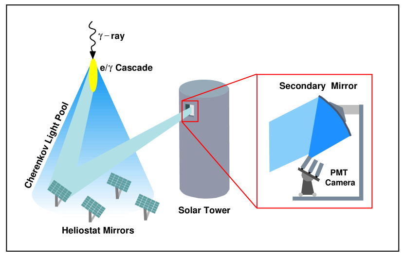
Figure 1: Concept of the central tower gamma-ray detector. Cherenkov light from the air shower initiated by the incident gamma ray is directed by large heliostats towards secondary optics located on the tower. These optics focus the light from each heliostat onto a corresponding photomultiplier tube.

2.1 Heliostats and Secondary Optics

There are 212 heliostats in the NSTTF array, each with a mirror area of $37~{}m^{2}$. STACEE uses 64 heliostats distributed throughout the field, as shown in figure 2, and grouped into eight clusters of eight heliostats each. Light from the heliostats is directed towards a central tower where five secondary mirrors and associated cameras are located. Three cameras, each with 16 channels, are located at the 160-foot level of the tower and two more, each with eight channels, are located at the 120-foot level. Each camera is at the focal point of a spherical f-1.0 secondary mirror (2.0 m diameter for the 16-channel cameras and 1.1 m diameter for the 8-channel cameras) which collects and focusses Cherenkov light reflected from the heliostats onto PMTs in the camera. Light concentrators coupled to the PMTs increase their effective areas and define their fields of view.

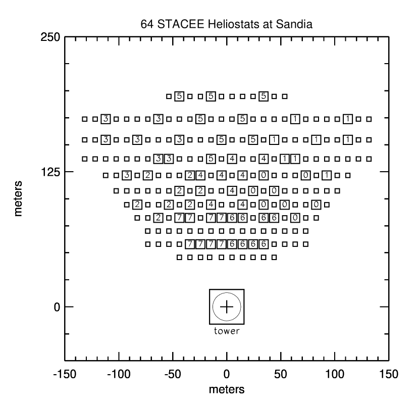
Figure 2: Map of the STACEE heliostat field. Each square denotes a heliostat and the ones used by STACEE are numbered from 0 through 7, according to the trigger cluster to which they are assigned. The orientation of the field is such that the heliostat rows are in an east-west direction and the tower is on the southern edge.

2.2 Electronics and Trigger

Pulses from the PMTs are first sent to high-speed amplifiers where the signal size is increased. Each amplifier channel produces two outputs; one is sent to a discriminator, followed by digital trigger logic and the other is digitized by an 8-bit flash analog-to-digital converter (FADC) (Acqiris DC-270) operating at 1 GS/s. The front-end amplifiers are commercially available NIM modules (Phillips 776). Two units, each with a gain of 10, are cascaded for each PMT.

The trigger is a custom-made device which uses field-programmable-gate-arrays (FPGAs) to delay each pulse (to account for the relative geometry of the Cherenkov wavefront and the heliostats) and require a majority coincidence of PMT signals to form a first-level trigger. The delays are dynamic; because of the earth’s rotation, a given source appears to move across the sky, so the relative timing of each channel needs to be continuously modified to maintain a tight trigger coincidence window. STACEE uses a window of 12 ns effective width. To keep the inter-channel delays reasonably short, the trigger operates in two stages. For the first stage, the 64 channels are grouped into eight groups of eight channels, corresponding to heliostats that are close together on the field (see figure 2). A given number of these channels (typically five) in a group is required to be above threshold for that group to trigger. For the second stage a given number of groups (also typically five) is required to fire before reading out the detector. This two-stage requirement has the effect of selecting light pools that are uniform over a large part of the heliostat field. Gamma-ray showers, which result in smooth light pools, are more likely to satisfy such a selection criterion than hadron-initiated showers, which tend to be clumpier.

3 Data Taking and Analysis

3.1 Observing Strategy

STACEE employs an ‘ON-OFF’  observing strategy. ‘ON’ runs of 28 minutes wherein the source is tracked at the centre of the field of view are alternated with ‘OFF’ runs where a patch of sky at identical declination but 30 minutes ahead or behind the source in right ascension is observed. The basic data unit is, then, a pair of such runs. The idea is that many backgrounds (for example terrestrial light sources) depend on local coordinates, and their effects will be the same in both runs. Additionally, and most importantly, the rate of background showers from charged cosmic rays will be the same for both runs, so that one can infer the gamma-ray flux from the difference in count rates between the two.

Each night, prior to taking data on a given source, special runs, where the trigger rate is measured as a function of increasing threshold setting, are performed. The trigger threshold is set just above the point where noise triggers, resulting from random coincidences of night sky background photons, cease to dominate the triggers from air showers. Typically we run at a threshold of 5-6 photoelectrons per channel. This number depends on atmospheric conditions, which affect the amount of scattered light.

3.2 Data Quality Cuts

Data analysis proceeds in stages. As part of the first stage, runs where weather conditions were poor are rejected, as are those where log files reveal periods of unstable tracking by one or more heliostats. Initial offline analysis also involves comparing the two runs of a pair. Count rates and currents for each channel and trigger group are required to be consistent between the two runs. Portions of runs where such quantities are not consistent are eliminated from further analysis. This criterion is applied to both runs of a pair; for example, if a cluster trigger rate is essentially constant for one run but deviates for a short time during the other run of the pair ($e.g.$ due to the passage of an airplane or a small cloud), the offending interval is removed from both runs.

3.3 Field Brightness Correction

A very important analysis task is that of correcting for the relative brightness of the ON and OFF fields. The effect is well-known in ground-based gamma-ray astronomy and different methods have been used by different groups to cope with it [16].

The ON-OFF observing strategy assumes that the difference between the total number of events from the ON run and that from the OFF run is due to a flux of gamma rays from the targeted source. Any background suppression and other analysis techniques are primarily used to improve the statistical significance of the gamma-ray excess. However, if the night-sky background (NSB) is different for the two observing fields, $e.g.$ due to one or more bright stars in one of the fields, a difference in count rates can arise from promotion effects. Promotion occurs when an air shower, having deposited enough Cherenkov light in the various channels of the detector to be just below threshold, is raised over threshold by the addition of one or more NSB photons which arrive during the trigger window. If the extra brightness is in the ON field, a spurious signal can develop or, if it is in the OFF field, a genuine signal can be lost or weakened. With STACEE data we correct for this effect using the FADC traces. In the following discussion we will assume that the ON field has the extra NSB.

An obvious solution to correct for a brighter ON-source field would be to add extra photo-electron signals, corresponding to the ON-OFF difference in photo-currents, to the OFF-field traces for each channel. This technique is called ‘software padding’. One could do this with simulated single photo-electron waveforms, but a detailed understanding of the pulse shape and its fluctuations at low charge levels is required. Instead, we adopt an empirical approach. It is an observational fact that, because of the AC coupling at the front end of the FADC and the high rates of NSB photons, which result in pile-up effects, the baseline FADC trace looks very much like random noise and can be well described by a single parameter, its variance. It is also true that the variance is linearly related to the photo-current. To equalize the ON and OFF FADC traces in a given channel, we compute the difference in baseline variance between ON and OFF and add an additional FADC trace having this variance to the OFF trace. By construction, the ON and OFF FADC baseline traces now have equal variances but any coherent air shower signal has not been affected.

The added trace is taken from a large library of such traces. The library traces are made by illuminating a PMT with a variable intensity light-emitting diode and triggering the read-out with a pulse generator. Thus the traces contain only controlled levels of baseline fluctuations. This technique is called ‘library padding’and was first used in [17]; the concept is illustrated schematically in figure 3.

Figure 3: Schematic illustration of the ‘library padding’ concept. An FADC trace with appropriate baseline variance, taken from a library of such traces, is added to the trace from a given event and channel to produce a pulse with larger baseline variance. All variances are calculated from the portion of the FADC trace which precedes the triggered pulse.

The padding process is followed by a re-imposition of the trigger in software. This must be done using a higher threshold than was used during data collection because, even though the OFF field has now been artificially brightened, any sub-threshold showers that would have triggered the experiment had the brightness been there in the first place cannot be recovered; they are not in the data set. Thus one must remove the corresponding showers from the ON-field data. The increment to the trigger threshold has been empirically determined by examining a series of ON-OFF pairs taken with bright stars of different magnitudes.

3.4 Hadron Rejection

After the data quality criteria are applied, we are left with data sets made up of series of triggered events, each containing 64 FADC traces, one per heliostat. Each trace is 192 samples long and contains the digitized primary PMT pulse near its centre. The times and charges of the pulses are extracted from these traces to be used in later analysis steps and the traces themselves are used in the hadron rejection process.

One of the most important steps in the analysis is that of rejecting showers caused by charged cosmic rays, henceforth called hadronic showers. We are working with a set of air showers where the ratio of gamma-induced air showers to hadronic showers is very small, the exact ratio depending on the gamma-ray source being observed. As stated earlier, the flux of gamma rays can be estimated from the ON-OFF count rate difference, but it is important to improve on the gamma/hadron ratio to enhance the statistical quality of this estimate.

STACEE is not an imaging detector, so the powerful hadron rejection techniques devised for such detectors [18] cannot be applied to our data. Instead, we use a scheme [19] referred to here as the grid alignment technique, for reasons that will become clear. This method was adapted for use in STACEE [20, 21], and has been tested using observations of the Crab Nebula [21, 22] where it has been shown to improve the signal from a 4.8 $\sigma$ excess to 8.1 $\sigma$ in our 2002-2004 data set. Stated differently, our sensitivity to the Crab is 1.62 $\sigma/\sqrt{hour}$. This is to be contrasted to the sensitivity obtained during our first observation of the Crab [23] with the STACEE-32 detector [14] which was 1.03 $\sigma/\sqrt{hour}$.

Gamma/hadron separation using the grid alignment technique relies on the difference in shapes between the wavefronts of gamma-induced showers and hadronic showers at the energies of interest to STACEE. By ‘wavefront’, we mean the distribution in space and time of the Cherenkov photons which arrive at the detector. Simulations show that gamma-induced showers have a smooth wavefront with a shape that forms part of a sphere, the origin of which is at the position of shower maximum, the point at which the population of particles in the air shower reaches its maximum value. Shower maximum is approximately 10-12 km above the detector for vertically incident gamma-ray showers. By contrast, hadronic showers have much more sub-structure and their wavefronts are not usually spherical. Calculating and selecting on the sphericity of showers is expected to be a useful tool in rejecting hadronic showers.

To calculate sphericity it is necessary to know where the core of the shower landed in the heliostat field. This is the point at which the incident gamma ray would have impacted the field had it not interacted in the atmosphere and initiated the shower. The core position is a priori unknown; for purposes of trigger timing, it is assumed to be at the centre of the field, but its true value can be quite far away since timing tolerances in the STACEE trigger allow for a range of values. To estimate more precisely the core position, we step through a grid of possible locations. At each point on the grid we calculate the time of arrival of the wavefront at each heliostat based on the geometry given by the core position and the location of shower maximum, assuming that it lies on the line connecting the core position and the targeted source. The position of shower maximum along the line is adjusted for atmospheric depth according to the elevation angle of the source. The differences of the expected arrival times from their observed values are used to shift the start times of each FADC trace and the traces are then summed. For the correct core position, pulses from the different heliostats will add coherently and produce a summed pulse with large amplitude and narrow width. (See figure 4.) For an incorrect core position, the amplitude will be smaller and the width will be larger, as shown in figure 5. The ratio of amplitude (height $H$) to width ($W$) of the summed pulses is used as a figure of merit in the following steps and it is assumed that the hypothesized core position which maximizes $H/W$ is the best estimate of the true core position.

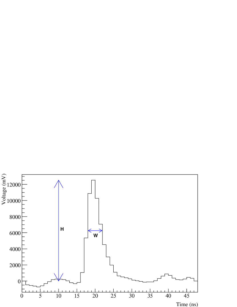
Figure 4: Sum of all FADC traces for a single, simulated, gamma-ray event. The quantities, $H$ and $W$, used in the grid ratio method of hadron rejection are shown by way of illustration. This plot was made using the position of the shower core that gives the largest value of $H/W$. Note that, before summing, all traces are pedestal-subtracted and inverted.

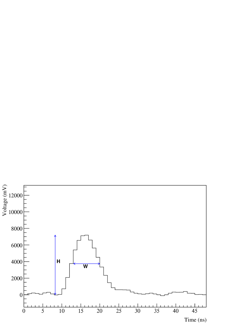
Figure 5: As in the previous figure but made with a shower core position 200 metres from the optimal position used in the previous figure.

To find the core position, a 30x30 grid with 15 m pitch is stepped through and the location with the maximum value of $H/W$, $H/W_{max}$, is saved. For gamma-ray showers one expects a peaked distribution of H/W values, as seen in figure 6 where the concept is illustrated using data from a simulated gamma-ray event.

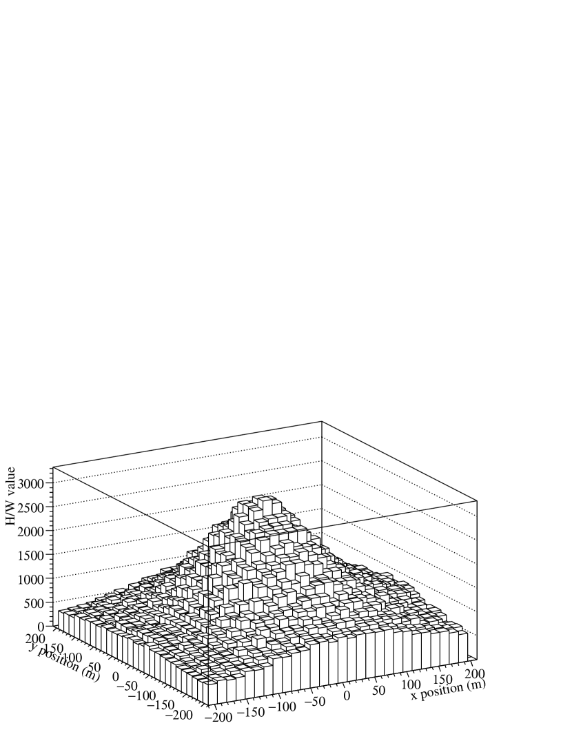
Figure 6: Illustration of the behaviour of the height-to-width ratio for the sum of FADC traces as a function of hypothesised shower core locations. This plot corresponds to a single simulated gamma-ray event and shows the characteristic peaking and symmetric behaviour expected of an electromagnetic shower with a spherical wavefront.

Hadronic showers are not expected to exhibit strong peaking, as shown in figure 7 where the $H/W$ distribution for a typical hadronic shower is shown. To quantify the flatness of the grid distribution, we calculate $H/W$ for four separate core locations, each 200 m distant from the best core estimate, along orthogonal axes perpendicular to the shower axis. (200 m was chosen as appropriate to the size of the heliostat array.) The average of these four values, $H/W_{200}$, is used to make the ratio $\xi=\frac{H/W_{200}}{H/W_{max}}$.

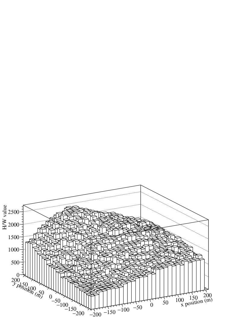
Figure 7: Illustration of the behaviour of the height-to-width ratio of a single simulated proton shower.

The difference in $\xi$ values for showers due to gamma rays and those initiated by protons is evident in figure 8 where simulations performed on a Crab-like spectrum ($E^{-2.4}$) at the Crab transit position are shown. Gamma-ray showers have, on average, lower values of $\xi$ than do proton showers. Part of this is due to the curvature of the wavefront, as discussed, but there is also an effect coming from the thickness of the shower front, which is smaller for gamma-ray showers. The quality factor, $Q$, defined as $Q=\frac{N^{\prime}_{\gamma}/N_{\gamma}}{\sqrt{N^{\prime}_{h}/N_{h}}}$ with the primed quantities being those passing a cut on $\xi$, is shown as a function of the cut value in figure 9. A cut value of $\xi<0.325$ gives the best $Q$ factor (2.6) but only retains 40% of the gamma rays. We use a slightly looser cut of $\xi<0.35$ which keeps 60% of the gamma rays.

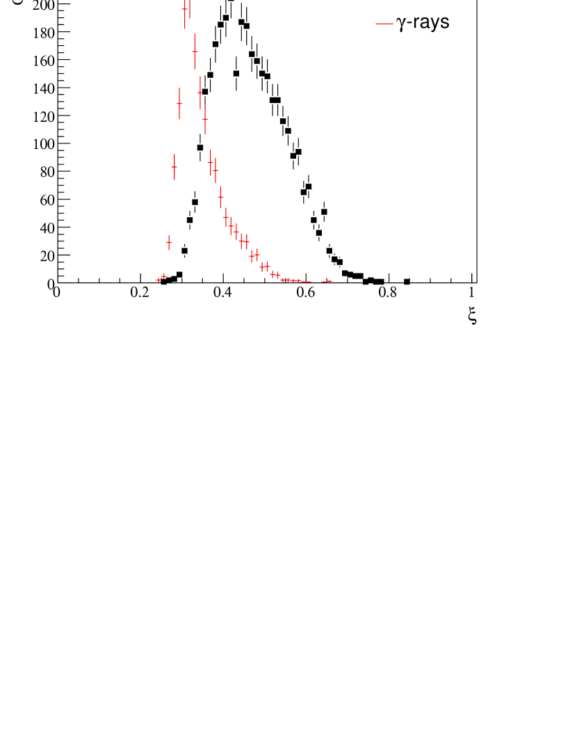
Figure 8: Distribution of the variable $\xi$ (defined in the text) from simulations of gamma rays and protons at the Crab transit point. The curves have been normalized to have the same maximum value.

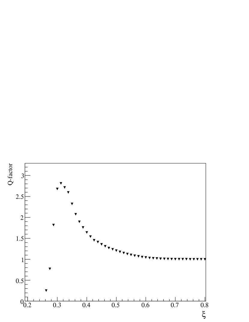
Figure 9: Quality factor $Q$ as a function of $\xi$ cut value, where $Q=\frac{N^{\prime}_{\gamma}/N_{\gamma}}{\sqrt{N^{\prime}_{h}/N_{h}}}$ with the primed quantities being those passing the cut, and the data are from simulations made at the Crab transit point.

As might be expected, there are several biases inherent in the grid ratio technique. The variable $\xi$ depends slightly on energy over the range explored by STACEE; its mean value for gamma rays rises from 0.32 at 100 GeV to 0.38 at 1000 GeV. It also depends on the position of the source on the sky since the depth of shower maximum depends on source elevation. Finally, due to the close packing, and close proximity to the tower, of heliostats in the southern part of the field (see figure 2), showers with a large fraction of their light hitting those heliostats have systematically larger values of $\xi$, an effect that must also be accounted for.

For the purposes of this work, we need to understand these biases and their effect on the acceptance of the STACEE detector as a function of energy and direction. We rely on extensive simulations to produce curves like that shown in figure 10 which illustrates, for a representative data set (2004 Mrk 421 data), the effective area of STACEE as a function of energy with different cuts applied to the data [21]. Clearly there are two large effects. At low energies, the increased pulse-height threshold that is part of the software padding process reduces the acceptance below 100 GeV. At high energies, the $\xi$ cut lowers the acceptance appreciably above 1 TeV. This effect is due to the fact the wavefronts of gamma-ray showers are less spherical at higher energies.

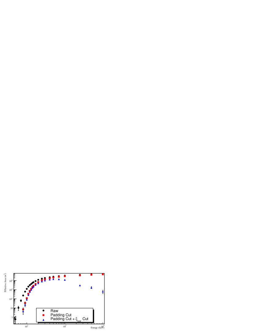
Figure 10: Effective area of the STACEE detector as a function of gamma-ray energy with different cuts applied to the data. Software padding, with its increase in threshold, affects the low energy range while hadron suppression lowers the acceptance at high energy.

For the two BL Lac objects observed by STACEE, we calculated separate, source-specific, versions of figure 10. All these acceptance curves are hour-angle-weighted; an acceptance curve was calculated for each of a set of different pointings and these were combined in an average, weighted according to how long was spent at each pointing.

In summary, the analysis selects data taken under conditions of acceptable weather with reliable hardware. ON/OFF field brightness differences are removed using library padding and hadronic showers are suppressed using the grid ratio technique. At this point a signal, manifest as a difference between ON and OFF count rates, is sought.

4 Results

4.1 3C 66A

The Third Cambridge (3C) radio survey at 159 MHz [24] resulted in a catalog of 471 sources in the northern hemisphere. It was later found that the source numbered 66 was composed of two unrelated objects, a BL Lac object now identified as 3C 66A and a radio galaxy, 3C 66B. The BL Lac classification has been supported by optical and X-ray observations.

3C 66A is coincident with the EGRET source 3EG 0222+4253 [6], but there are other objects in the EGRET error box, including the pulsar J0218+4232. It has been suggested by Kuiper $et~{}al$ [25] that the pulsar contributes to the observed gamma-ray flux at energies less than 500 MeV while the BL Lac object dominates at higher energies.

No confirmed detections of this source have been made at very high energies. A result from the Crimean GT-48 telescope [26] has not been confirmed. Indeed, measurements in the same energy range have resulted in upper limits [27, 28], that are lower than the flux reported by the GT-48 group. However it is always important to remember that BL Lac objects are highly variable so a non-confirmation is not necessarily a contradiction.

STACEE observed 3C 66A from September to December, 2003 as part of a multi-wavelength campaign summarized in Boettcher $et~{}al$ [29]. We acquired a data set of 87 ON/OFF pairs. Weather and hardware quality cuts removed 31% of the data, leaving an ON source live-time of 83.2 ks. These data have been analysed and presented before [7], but without applying hadron rejection.

Figure 11 shows the $\xi$ distributions for the ON and OFF data sets and figure 12 shows the difference. There is no evidence for a signal. Applying the $\xi<0.35$ cut results in a net rate of $-0.35\pm 0.22$ counts per minute, which is 1.6 standard deviations below background. Since this is consistent with zero we calculate a bounded upper limit for the rate. The $99\%$ CL upper limit on the gamma-ray rate is 0.37 counts per minute.

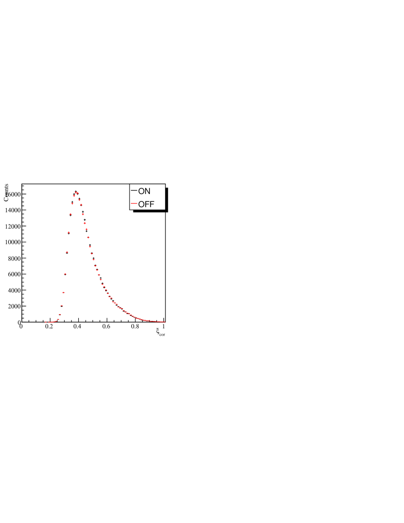
Figure 11: Number of showers, as a function of the grid ratio cut variable $\xi$, for the 3C 66A data. The ON and OFF data are essentially overlapping.

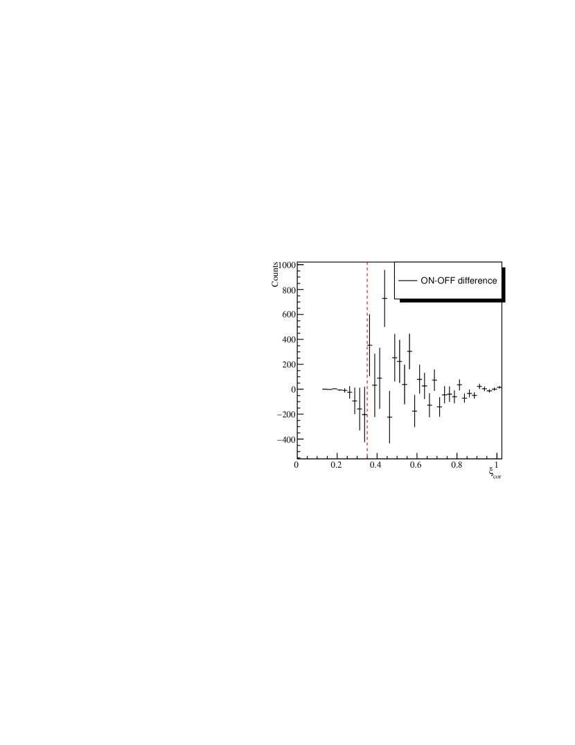
Figure 12: The difference of the two curves plotted in the previous figure. The dashed line indicates the value below which gamma-ray events are expected.

To calculate an upper limit for the flux, we must make assumptions about the spectrum of 3C 66A. Since most VHE sources exhibit power law behaviour over the range of our sensitivity, we adopt such a form. However, it is worth remembering that, depending on the distance of the source, EBL attenuation effects can cause a steepening of the spectrum at high energies and that this can affect our calculated limit. The choice of spectral index is not well constrained; we choose a value of 2.5, which is typical for the detected VHE blazars. We recognise that our result is tightly correlated to this value.

Assuming the spectral form, $dN/dE=N_{0}(E/E_{0})^{-2.5}$ and convoluting it with the effective area $vs$ energy curve results in the response curve shown in figure 13. It is customary in VHE gamma-ray astronomy to define the peak value of this curve to be the energy threshold. According to this definition, the energy threshold for this measurement is $185$ GeV, with a systematic uncertainty of $45$ GeV.

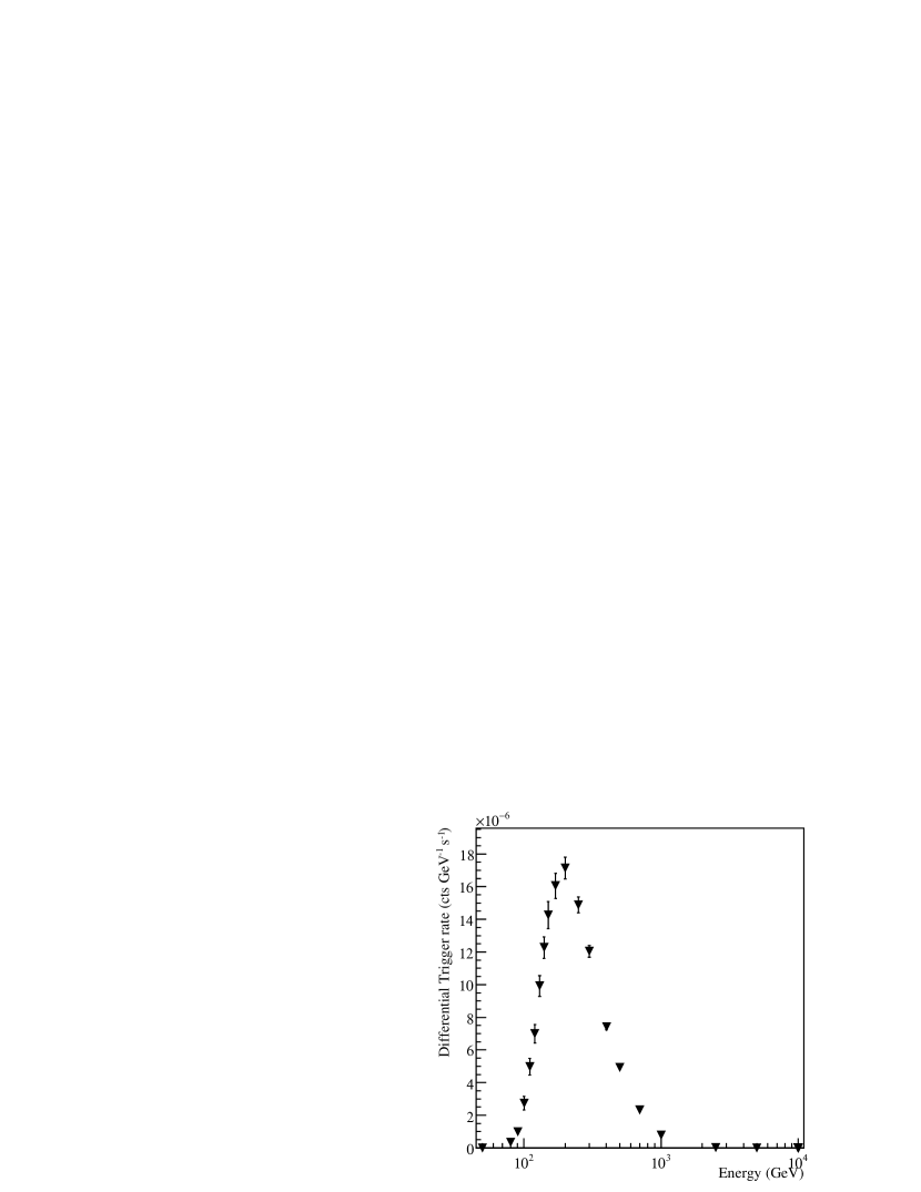
Figure 13: The convolution of power law energy spectrum (spectral index = 2.5) with the hour-angle weighted effective area curve for the 3C 66A data set. The peak at 185 GeV provides an operational definition of the energy threshold.

Our 99% CL upper limit on the gamma-ray flux at 185 GeV is $E^{2}dN/dE$ (185 $\pm 45_{sys}$ GeV) $<1.1\times 10^{-4}$ GeV m^-2s^-1. Stated differently, we can say that the 3C 66A integral gamma-ray flux above 185 GeV is less than 15% of that of the Crab Nebula, using results from STACEE measurements of the Crab over the same energy range ([30]). As can be seen in figure 14, this upper limit is approximately three times lower than our previous result [7] due to the improved hadron rejection afforded by the grid ratio technique. However, it is still well above the flux value obtained by interpolating the predictions found in the study by Costamante and Ghisellini [1]. Our point is above those from the imaging Cherenkov telescopes, Whipple and HEGRA, but it is at a lower energy, where the EBL absorption of photons from this distant source is expected to be less important.

The EGRET measurement shown in the figure is actually from the source 3EG 0222+4253 which includes the pulsar J0218+4232 [25] as well as 3C 66A. It is not clear how much of the observed flux can be attributed to 3C 66A alone.

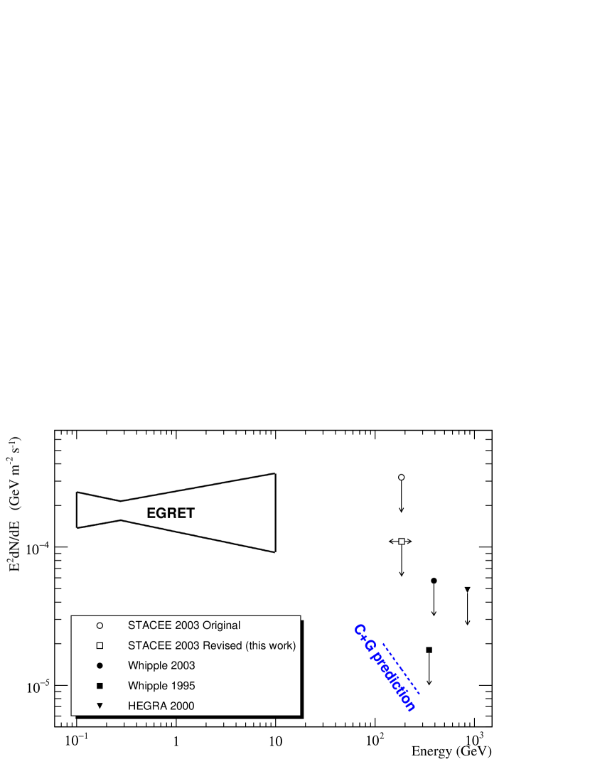
Figure 14: The spectral energy distribution for 3C 66A in the gamma-ray region. Note that all small symbols denote upper limits. The STACEE limit (revised) has been improved using the technique described in this paper. The EGRET symbol corresponds to data from 3EG 0222+4253 which includes 3C 66A but also a pulsar.

4.2 OJ 287

OJ 287 was discovered in 1968 in the Ohio State University survey of radio sources at 1415 MHz [31]. It was soon identified with an optical source of magnitude 14.5 [32] and further work at other wavelengths established its membership in the BL Lac class [33]. Its redshift has been measured to be 0.306 [34, 35].

Optically, OJ 287 has been followed for more than 100 years. It appears to have a marked increase in optical emission every twelve years, a phenomenon that can be explained by supposing that the AGN contains a pair of orbiting black holes, a primary with mass $10^{10}~{}M_{\bigodot}$ and a secondary with mass $10^{7}~{}M_{\bigodot}$ [36]. The last outburst occured in 1994-95, and it was during this time that EGRET accumulated most of its observing time on the source. EGRET detected OJ 287 as a relatively weak source with an average integral flux of $10.6\pm 3.0\times 10^{-8}$ photons cm^-2 s^-1 [6]. This source has not been detected by any of the VHE telescopes.

STACEE observed OJ 287 from December, 2003 to February, 2004 and obtained a data set of 28 ON/OFF pairs. After weather and other quality cuts were applied, 52% of the data remained, corresponding to 21.1 ks of ON-source live time. The distributions of $\xi$ for ON and OFF are very similar to those shown in figure 11 and the difference distribution resembles figure 12. The standard $\xi$ cut results in a flux of 0.35 $\pm$ 0.39 counts min^-1 and a statistical significance of 0.9 standard deviations above background. As with 3C 66A, we use these numbers to calculate a 99% CL upper limit on the gamma-ray rate. This upper limit is 1.29 photons per minute. Using the hour-angle-weighted effective area curve and assuming a power law spectrum with index of 2.5, we obtain an energy threshold of 145 $\pm$ 36 GeV and a gamma-ray flux upper limit of $E^{2}dN/dE$ (145 $\pm 36_{sys}$ GeV) $<4.0\times 10^{-4}$ GeV m^-2s^-1. This corresponds to 52% of the Crab Nebula flux above the same energy.

The spectral energy distribution, as measured by EGRET and with the STACEE limit and Costamante and Ghisellini prediction included, is shown in figure 15. It is seen that our measurements are above the Costamante and Ghisellini prediction but are the only ones reported at these energies.

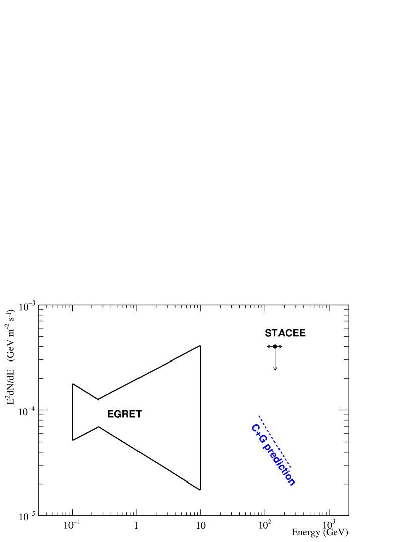
Figure 15: The spectral energy distribution for OJ 287 in the gamma-ray region.

5 Conclusions

We have presented data from recent STACEE observations of two of the three LBL candidates suggested as potential TeV emitters by Costamante and Ghisellini [1]. We have not detected a signal from either of these sources and have set upper limits on their gamma-ray flux levels. Although the sensitivity of STACEE has been improved through the use of a new hadron rejection technique, also presented in this paper, we cannot rule out emission at the level suggested in [1]. Although neither of the sources has yet been detected in the VHE range, the third LBL candidate, BL Lacertae has recently been detected by the MAGIC collaboration [2]. Their results indicate that BL Lacertae is highly variable, as is typical for most blazars. We look forward to improved limits or detections now that a new generation of ground-based detectors, VERITAS [37] and MAGIC [38], are viewing the northern sky with improved sensitivity and lower energy thresholds.

6 Acknowledgements

We are grateful to the staff at the National Thermal Solar Test Facility for their enthusiastic and professional support. This work was funded in part by the U.S. National Science Foundation, the University of California, Los Angeles, the Natural Sciences and Engineering Research Council, le Fonds Québecois de la Recherche sur la Nature et les Technologies, the Research Corporation, and the California Space Institute.

References

- [1] L. Costamante and G. Ghisellini, Astronomy and Astrophysics 384: 56 (2002)
- [2] J Albert et al, arXiv:astro-ph/0703084v1 (2007)
- [3] T.C. Weekes et al, Astrophys. J. 342, 379 (1989)
- [4] R.A. Ong, Rapporteur Talk, 29th Int. Cosmic Ray Conference, (Pune), (2005)
- [5] M. Punch et al, Nature 358, 477 (1992)
- [6] R.C. Hartman et al, Astrophys. J. Supp. 123, 79 (1999)
- [7] D.A. Bramel et al, Astrophys. J. 629, 108 (2005)
- [8] F.W. Stecker et al, Astrophys. J. Lett. 390, L49 (1992)
- [9] E. Pare et al, Nucl. Instrum. and Meth. A490: 71 (2002)
- [10] F. Aqueros et al, Astroparticle Physics 17: 293 (2002)
- [11] P. Marleau, Proc. Towards a Network of Atmospheric Cherenkov Detectors VII, Palaiseau 2005
- [12] D.A. Smith, Proc. Towards a Network of Atmospheric Cherenkov Detectors VII, Palaiseau 2005
- [13] M.C. Chantell et al, Nucl. Instrum. and Meth. A408: 468 (1998)
- [14] D.S. Hanna et al, Nucl. Instrum. and Meth. A489: 126 (2002)
- [15] D.M. Gingrich et al, IEEE Transactions on Nuclear Science 52 2977 (2005)
- [16] M.F. Cawley, Proc. Towards a Major Atmospheric Cherenkov Detector II, Calgary, 1993
- [17] R.A. Scalzo et al, Astrophys. J. 607, 778 (2004)
- [18] A. Hillas. Proc 19th 29th Int. Cosmic Ray Conference (La Jolla) 3: 455 (1985)
- [19] D.A. Smith et al, A&A 459, 453 (2006)
- [20] J. Kildea et al, Proc 29th Int. Cosmic Ray Conference (Pune) 5: 135 (2005)
- [21] T. Lindner, PhD thesis, McGill University (2006), unpublished
- [22] J. Kildea et al, Proc 29th Int. Cosmic Ray Conference (Pune) 4: 89 (2005)
- [23] S. Oser et al, Astrophys. J. 547, 949 (2001)
- [24] D.O. Edge et al, MmRAS 68: 37 (1959)
- [25] L. Kuiper et al, A&A 359, 615 (2000)
- [26] A.A. Stepanyan et al, Astronomy Reports 46: 634 (2002)
- [27] D. Horan et al, Astrophys. J. 603, 51 (2004)
- [28] F. Aharonian et al, A&A 421, 529 (2004)
- [29] M. Boettcher et al, Astrophys. J. 581, 143 (2002)
- [30] P. Fortin, PhD thesis, McGill University (2005), unpublished
- [31] R.S. Dixon and J.D. Kraus, Astronom. J. 73: 381 (1968)
- [32] G.M. Blake, Astrophys. Lett. 6: 201 (1970)
- [33] P.A. Strittmatter et al, Astrophys. J. 175, L7 (1972)
- [34] J.S. Miller et al, Proc. Pittsburgh Conf. on BL Lac Objects, (A79-30026) (1978)
- [35] M.L. Sitko and V.T. Junkkarinen, Astron. Soc. of the Pacific, Publications 97: 1158 (1985)
- [36] A. Sillanpää et al, Astrophys. J. 325, 628 (1988)
- [37] J. Holder et al, Astroparticle Physics 25: 391 (2006)
- [38] E. Lorenz, New Astr. Rev. 48: 339 (2004)