Synchrotron flaring behaviour of Cygnus X-3 during the February–March 1994 and September 2001 outbursts

Abstract

Aims. In this paper we study whether the shock-in-jet model, widely used to explain the outbursting behaviour of quasars, can be used to explain the radio flaring behaviour of the microquasar Cygnus X-3.

Methods. We have used a method developed to model the synchrotron outbursts of quasar jets, which decomposes multifrequency lightcurves into a series of outbursts. The method is based on the Marscher & Gear (1985) shock model, but we have implemented the modifications to the model suggested by Björnsson & Aslaksen (2000), which make the flux density increase in the initial phase less abrupt. We study the average outburst evolution as well as specific characteristics of individual outbursts and physical jet properties of Cyg X-3.

Results. We find that the lightcurves of the February–March 1994 and September 2001 outbursts can be described with the modified shock model. The average evolution shows that instead of the expected synchrotron plateau, the flux density is still increasing during the synchrotron stage. We also find that high frequency peaking outbursts are shorter in duration than the ones peaking at lower frequencies. Finally, we show that the method can be used, complementary to radio interferometric jet imaging, for deriving the physical parameters such as the magnetic field strength and the energy density of relativistic electrons in the jet of Cyg X-3.

1 Introduction

X-ray binary systems exhibiting jets with relativistic motions are called microquasars. They are generally regarded as the galactic counterparts of more powerful extragalactic sources, quasars. This suggests that the underlying physical processes that operate in these systems are the same and thus are manifested in their radiative processes.

Cygnus X-3 is one of the most intensively studied microquasars. It is a strong X-ray source, and is thought to consist of a compact object accreting matter from a Wolf-Rayet star (van Kerkwijk et al. 1996). The source occasionally undergoes huge radio outbursts in which the flux density can increase up to levels of $\sim 20$ Jy at frequencies of a few GHz. The radio flares more typically consist of a few peaks of 1-5 Jy and are preceded by a quenched state (Waltman et al. 1994). During recent outbursts, jet-like structures have been observed at radio frequencies. On milliarcsecond scales a one-sided jet was observed with the Very Long Baseline Array (VLBA) during one outburst of February 1997 (Mioduszewski et al. 2001, hereafter M01) while in September 2001 a two-sided jet was observed (Miller-Jones et al. 2004, hereafter MJ04). On arcsecond scales a two-sided jet has been observed with the Very Large Array (VLA) in September 2000 (Martí et al. 2001).

The synchrotron emission of microquasars has historically been interpreted as originating from distinct expanding clouds of relativistic plasma (van der Laan 1966, Hjellming & Johnston 1988). More recently, the internal shock model – originally developed for $\gamma$-ray bursts – has been suggested to explain the observed variability of microquasars (Kaiser et al. 2000). On the other hand, the model of Marscher & Gear (1985) – describing analytically the synchrotron emission of a shock wave propagating downstream in a relativistic jet – has been the baseline model for the flaring behaviour of quasars in the radio-to-submillimetre range. Recently, this shock wave interpretation has been shown to be able to describe well the observed lightcurves of two microquasars: GRO J1655-40 (Hannikainen et al. 2000, Stevens et al. 2003) and GRS 1915+105 (Türler et al. 2004).

In this work we study a third galactic source, Cyg X-3, showing repeated outbursts with a typical evolution from high- to low-frequencies as expected by the model of Marscher & Gear (1985) but with significantly longer outbursts than in GRS 1915+105. We use a generalization of the shock-in-the-jet model of Marscher & Gear (1985) to describe two distinct flaring epochs of Cyg X-3: February–March 1994 and September 2001. We decompose simultaneously the multifrequency lightcurves into a series of outbursts using a similar methodology as for 3C 273 (Türler et al. 1999, 2000), GRS 1915+105 (Türler et al. 2004) and 3C 279 (Lindfors et al. 2005, 2006). Preliminary results on the February–March 1994 period were already published in Lindfors & Türler (2007).

This method allows us to derive the observational and physical properties of an average outburst in our data set. We then use this result to further probe the physical conditions of the emission region in the jet of Cyg X-3.

2 Data

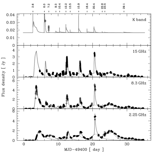
Figure 1: Lightcurves of the February–March 1994 outburst decomposed into a series of 13 outbursts. The solid line shows the sum of all components and dashed lines separate the contribution of individual outbursts. The radio lightcurves are from the Ryle telescope (15 GHz) and the GBI (2.25 GHz and 8.3 GHz) while the infrared data are from the UKIRT. Any additional constant quiescent flux is assumed to be negligible except for the K-band lightcurve, where we fix it to 16.6 mJy according to Fender et al. (1996). The time labels at the top of the figure show the starting dates of the outbursts.

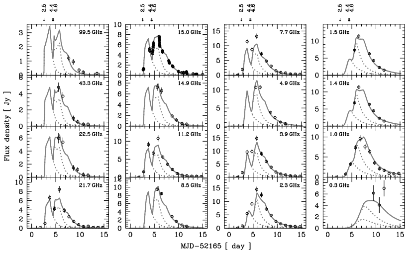
Figure 2: Sixteen lightcurves of the September 2001 flaring period decomposed into a series of three distinct outbursts. The solid line shows the sum of the model outbursts and dashed lines separate the contribution from individual events. The time labels at the top of the figure show the starting dates of the outbursts. The data are from VLA (0.3275, 1.385, 1.465, 4.86, 8.46, 14.94, 22.46, 43.34 GHz), RATAN 600 (1.0, 2.3, 3.9, 7.7, 11.2 and 21.7 GHz), Ryle Telescope (15 GHz) and OVRO (99.48 GHz).

In February–March 1994 Cygnus X-3 was observed to be flaring at radio frequencies. The flaring lasted for approximately 30 days during which time the radio flux density increased and decreased several times. The maximum flux density of this flaring epoch was $\sim 5$ Jy at 2.25 GHz. The dataset used here has been published by Fender et al. (1997). It contains radio lightcurves from the Ryle telescope at 15 GHz and from the Green Bank Interferometer (GBI) at 2.25 GHz and 8.3 GHz and infrared data from the United Kingdom Infrared Telescope (UKIRT). A possible constant emission in Cyg X-3 during quiescence is much smaller than the peaks of the flares and hence can be considered negligible in the radio, but not in the infrared. We therefore assume a quiescent flux density contribution in the K-band of 16.6 mJy as measured on 7 August 1984 (Fender et al. 1996).

In September 2001 Cyg X-3 underwent a major flare with flux densities reaching 15 Jy at 4 GHz. This flaring period was quite different from the one of February–March 1994: the maximum flux density is much higher and judging from the lightcurves it seems that it consists of only 2 to 3 distinct outbursts. For this flaring period we use data from 16 frequencies. They are composed of the Very Large Array (VLA, 0.3275, 1.385, 1.465, 4.86, 8.46, 14.94, 22.46, 43.34 GHz) and Owens Valley Radio Observatory (OVRO, 99.48 GHz) data published by MJ04, the RATAN 600 monitoring data at 1.0, 2.3, 3.9, 7.7, 11.2 and 21.7 GHz , and the 15 GHz lightcurve from the Ryle telescope. We noticed some calibration discrepancy between the VLA data and the RATAN 600 and Ryle telescope data. We therefore multiplied the VLA flux densities and errors by a factor 0.8 to match the flux density scale of the other datasets.

As our method consists in a $\chi^{2}$ fit of all data points simultaneously (see Sect. 3), data with smaller uncertainties will have more weight in the fit. If some lightcurves have much larger error-bars than others, they might not have enough weight to well constrain the model. It is therefore important to have lightcurves with comparable relative errors to get an equilibrated fit across the frequency range. We have, therefore, doubled the error estimates at 2.25 GHz for the 1994 dataset. The original uncertainties in the 2001 dataset are directly proportional to the flux. This results in very small errors for low-flux measurements and thus gives to those observations much more weight in the fit. To partly compensate for this effect we add systematic errors of 0.3 Jy to all data in the 1–22.5 GHz frequency range, 0.2 Jy at 43.3 GHz, and 0.1 Jy at 99.5 GHz.

3 Model and Method

The model we use to study the flaring behaviour of Cyg X-3 is based on the shock model of Marscher & Gear (1985). This model considers a disturbance - pressure or bulk velocity increase – at the base of the jet that will eventually become supersonic because of the pressure gradient along the jet. The resulting shock wave will accelerate particules crossing the shock front that will emit an outburst of synchrotron radiation in the increased magnetic field of the shocked plasma. Marscher & Gear (1985) identify three distinct phases during the downstream propagation of a shock wave in a jet and describe analytically the evolution of the associated synchrotron emission. In the initial growth phase, when the Compton losses predominate, the synchrotron self-absorption turnover frequency decreases and the turnover flux density increases. In the second phase the synchrotron losses dominate and the turnover frequency decreases while the turnover flux density remains roughly constant. The third phase is the decay phase, when the adiabatic losses dominate and both the turnover frequency and flux density decrease. Björnsson & Aslaksen (2000) proposed a modification to the initial Compton-loss stage making the initial rise in flux density much less steep than in the original calculation of Marscher & Gear (1985). The model used here takes this modification into account.

par.	description	value 1994	value 2001
$t_{\mathrm{r}}$	start time of the synchrotron stage	0.12 d	0.19 d
$t_{\mathrm{p}}$	time of peak flux density (start of adiabatic stage)	1.15 d	1.74d
$\nu_{\mathrm{p}}$	frequency of peak flux density	1.75 GHz	1.86 GHz
$S_{\mathrm{p}}$	peak flux density	1.93 Jy	10.74 Jy
$\nu_{\mathrm{b}}$	frequency of spectral break at time $t_{\mathrm{p}}$	115 GHz	122 GHz
$t_{\mathrm{f}}$	start time of optically thin slope flattening	0.03 d	0.04 d
$s$	index of electron energy distribution $N(E)\propto KE^{-s}$	1.77
$k$	index of electron normalization change $K\propto R^{-k}$	2.54
$r$	index of jet opening radius change with distance $R\propto L^{r}$	1.21
$b$	index of magnetic field strength change $B\propto R^{-b}$	1.57
$d$	index of Doppler factor change $D\propto R^{-d}$	0.0

Table 1: Physical and observational parameters describing an average outburst during the 1994 and 2001 flaring periods. The parameter $d$ was fixed to zero in our model. The ten remaining parameters have only been adjusted to the 1994 dataset, since we assume the same typical outburst evolution for the 2001 dataset (see text). We however give here the observational parameter values that we derive on average in 2001 according to the specificities of the 3 outbursts given in Table 2.

The generalized equations of the Marscher & Gear (1985) shock model were derived by Türler et al. (2000). This generalization allows one to describe the emission from shocks which are not necessarily propagating with constant velocity in a straight, conical and adiabatic jet. The synchrotron outburst is characterized by the frequency $\nu_{\mathrm{m}}$ and flux density $S_{\mathrm{m}}$ of the synchrotron self-absorption turnover evolving with time. As the jet opening radius $R\propto L^{r}$ is widening with distance along the jet $L$ and thus with time $t$ since the onset of the shock wave, the evolution of the observable quantities $\nu_{\mathrm{m}}$ and $S_{\mathrm{m}}$ is defined by the dependency on $R$ of physical jet quantities. These physical quantities are the normalization $K\propto R^{-k}$ of the electron energy distribution $N(E)\propto KE^{-s}$, the magnetic field strength $B\propto R^{-b}$ and the Doppler factor of the emission region $D\propto R^{-d}$. In the model used here for Cyg X-3 we do not allow for a change of the Doppler factor by fixing $d=0$.

To apply this model to the observations we use the methodology originally proposed by Türler et al. (1999, 2000). It consists in fitting iteratively subsets of all model parameters simultaneously to the complete observational dataset. The model parameters describe fully the synchrotron emission of a typical model outburst with a set of both physical and observational parameters (listed in Table 1) from which individual outbursts are only allowed to differ by their start time and by three additional parameters. These three outburst specific parameters can either define a scaling in time $t$, frequency $\nu$ and flux $S$ (Türler et al. 1999) or be the consequence of a more physical scaling of the quantities $K$, $B$ and $D$ defined above (Türler et al. 2000). We choose here for Cyg X-3 the more phenomenological approach also used recently for 3C 279 by Lindfors et al. (2006).

The model parameterization is simplified in Cyg X-3, because of the negligible underlying radio jet emission and the absence of a decaying outburst at the start of the flaring periods. We tested a model accounting for the emission from the receding jet, as was used for GRS 1915+105 (Türler et al. 2004), but this did not improve the fit and therefore we decided to use a simple model where all the emission originates from the approaching jet. The jet velocity $\beta=v/c$ and orientation $\theta$ to the line of sight derived from radio imaging observations (M01, MJ04) suggests that the condition $\beta\approx\cos(\theta)$ for having a shock viewed sideways is not satisfied (Marscher et al. 1992). We therefore use here the usual equations describing the evolution of a shock viewed face-on to the observer. Other differences compared to previous studies are that we do not impose here a linear decrease of the magnetic field $B$ with the jet opening radius $R$ as $B\propto R^{-1}$, and we do not include a spectral break below the synchrotron self-absorption turnover frequency. Indeed, we found that the lack of data in the submillimetre range, does not allow to well constrain this additional parameter during the early phase of the shock evolution. The optically thick spectral index is therefore fixed to 2.5 which is the theoretical value for a homogeneous synchrotron source.

4 Results and Discussion

We have decomposed the lightcurves of the February–March 1994 and September 2001 periods into a series of outbursts. The model for the February–March 1994 data has a total of 62 free parameters: 10 parameters are used to describe the shape and evolution of the synchrotron outburst (see Table 1), while the remaining 52 parameters are used to define the start times of the 13 outbursts as well as their specificity (see Table 2). The model fit to the 1994 lightcurves is shown in Fig. 1. The September 2001 dataset is rather sparsely sampled, and although it contains 16 frequencies, it has more than 10 times less data points than the 1994 dataset and therefore can only loosely constrain the model. We chose to fix the average evolution and jet parameters for the 2001 outbursts to those derived for the 1994 observations. The fit to the 2001 dataset has, therefore, only 12 free parameters, which are the start times and specificities of the three outbursts given in Table 2. The best fit model is shown for all 16 lightcurves in Fig. 2.

We obtain reduced $\chi^{2}$-values of $\chi^{2}$/d.o.f. = $\chi^{2}$/3314 = 10.2 and $\chi^{2}$/d.o.f. = $\chi^{2}$/261 = 1.80, for the 1994 and 2001 datasets, respectively. These values, above unity, reflect the fact that our fit is not able to fully describe any single data point. We however consider these values as adequate, because the prime goal of this study is not to have a perfect fit, but to derive the main physical properties of the jet based on the available observations. The model is therefore kept as simple as possible, in particular by assuming self-similar outbursts in a jet with constant physical properties. Furthermore, we do not consider here jet precession and counter-jet emission.

Visual inspection of the fit reveals that the model curve remains sometimes below the peaks of the observed lightcurves. This was also found for 3C 279 and is a known problem of shock-in-jet models – the model seems not able to reproduce well the sharp peaks of the observed lightcurves. However, this probelm could partly be due to the fact that errors are often proportional to flux so that the $\chi^{2}$ fit gives less weight to high-flux measurements compared to low-flux observations.

4.1 The Average Evolution of the Outbursts and Properties of Individual Outbursts

The overall evolution of an average model outburst in Cyg X-3 in February–March 1994 is shown in Fig 3 and corresponding parameter values are given in Table 1. The flux density increase during the Compton stage is rather slow but during the synchrotron stage the increase in flux density becomes more abrupt. The slow rise in the flux during the Compton stage is a consequence of the use of the modified outburst evolution for this phase proposed by Björnsson & Aslaksen (2000). The existence of this Compton stage and the location of the transition to the synchrotron stage are however only very loosely determined by the few infrared measurements. A direct transition to the adiabatic stage either from the synchrotron or the Compton stage, which are difficult to distangle, is therefore not excluded.

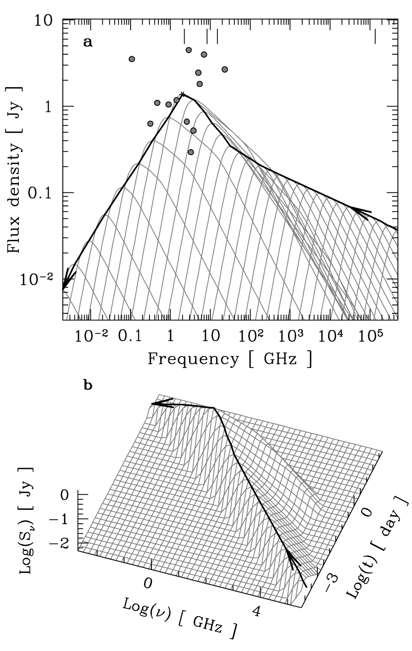
Figure 3: a) Series of model spectra at different times during the evolution of the average outburst. The filled circles refer to specific characteristics of individual outbursts of the February–March 1994 as listed in Table 2. b) The three dimensional evolution of the average outburst in logarithmic scale. The solid line with arrows shows the path followed by the spectral self-absorption turnover.

Individual outbursts differ from the average outburst by a rescaling in flux ($S$), frequency ($\nu$) and time ($t$). This rescaling is parameterized in the model by the logarithmic shifts given in Table 2. These shifts change the amplitude $S_{p}$, the peaking frequency $\nu_{p}$ and the duration $t_{p}$ of individual outbursts as shown by the filled circles in Fig. 3. To investigate whether the shifts are correlated, we applied the Spearman rank-order test (e.g. Press et al. 1992). For the February–March 1994 outburst, we find a significant anti-correlation (likelyhood for such correlation to appear by chance is less than 0.25%) between the peaking frequency and the duration, the highest peaking outbursts being shorter. The same behaviour was previously found in 3C 273 (Türler et al. 1999). As suggested by these authors this anti-correlation might be related to the distance from the core at which the shock forms, the short-lived and high-frequency peaking flares forming closer to the core than longer-living low-frequency peaking outbursts.

Because the 2001 flaring period consists of three outburst components only, any correlation study is not applicable there. Compared to the 1994 period, the outbursts of 2001 differ mainly in amplitude (flux density), while timescales and frequency ranges are similar (see Tables 1 and 2).

dataset	$T_{0}$	$\Delta$ log$S$	$\Delta$ log$\nu$	$\Delta$ log$t$
1994	2.6	0.46	0.54	-0.03
	6.0	0.29	1.06	-0.57
	7.2	-0.10	-0.63	0.07
	9.3	-0.42	0.28	-0.15
	10.4	-0.32	0.11	0.13
	12.2	0.25	0.40	-0.38
	13.5	-0.12	-0.35	0.36
	15.9	0.12	0.43	-0.43
	18.4	-0.07	-0.15	0.37
	20.4	0.51	0.16	-0.59
	22.8	0.41	-1.27	0.41
	23.5	-0.34	-0.80	0.62
	29.1	-0.67	0.21	0.18
2001	2.5	0.81	0.32	0.05
	4.4	0.76	-0.03	0.09
	4.6	0.67	-0.21	0.41

Table 2: The start times ($T_{0}$) of the model outbursts and their logarithmic shifts from the average shock evolution in flux density ($\Delta$ log $S$), frequency ($\Delta$ log $\nu$, negative if the outburst peaks at lower frequencies than the average outburst) and time scale ($\Delta$ log $t$, negative if the outburst evolution is faster than the evolution of the average outburst). The times $T_{0}$ are expressed in days starting from 17 Feb. 1994 (MJD-49400) and from 13 Sep. 2001 (MJD-52165) for the datasets of 1994 and 2001, respectively. The shifts of the September 2001 dataset are given with respect to the average model outburst derived for February–March 1994 dataset, because we chose to use the same typical outburst evolution and jet parameters for both datasets (see text).

4.2 Jet Properties

The jet parameters derived for Cyg X-3 are given in Table 1. We find a value of $k$ of 2.54, which is almost exactly what one would expect for an adiabatic jet flow $k_{ad}=2(s+2)/3\approx 2.51$. The derived value for $b$ suggests that the magnetic field is rather randomly oriented than purely perpendicular ($b=1.0$) or parallel ($b=2.0$) to the jet. The fact that the value of $r$ is found greater than 1 suggests that the jet opening angle increases with distance from the core. This was previously found for the other microquasar GRS 1915+105 analysed with the same method and is opposite to what we found for the quasars 3C 273 and 3C 279. If the microquasar jets are indeed trumpet-like (this was suggested already by Marti et al. 1992), it could be the result from the pressure gradient of material surrounding the jet or from diverging external magnetic field lines channelling the jet plasma. A high value of $r$ could also be the signature of a decelerating jet flow, but as for GRS 1915+105 we do not find a better fit by relaxing the value of $d$ to prove this hypothesis. As the effect of the high $r$ value is only to fasten the decrease of the spectral turnover frequency with time, Türler & Lindfors (2007) proposed an alternative origin for this behaviour. They discuss the possibility that the observed spectral turnover might not be the self-absorption turnover, as assumed here, but be the result of a low-energy cut-off in the electron spectrum. If the characteristic synchrotron frequency associated to the electrons with minimal energy would be higher than the synchrotron self-absorption frequency during the early stages of the outburst’s evolution, we would indeed have a faster evolution of the spectral turnover with time. However, further investigation of this alternative to the trumpet-like jet explanation is beyond the scope of this paper.

We find that in order to fit the data well, the electron index $s$ needs to be below 2.0, our best fit model having $s=1.77$. Such low $s$ values have been suggested for several AGNs by Valtaoja et al. (1988), Hughes et al. (1989, 1991) and Stevens et al. (1995, 1996) although traditionally such low $s$ values are disfavoured by theory as for $s<2$ the strong radiative losses of the dominant high-energy electrons would lead to a substantial pressure decrease along the jet and prevent the shock to propagate far (Marscher & Gear 1985).

However, recent theoretical work has shown that an index of $s<2.0$ can be explained with e.g. a high minimum energy of the electron energy spectrum (Katarzynski et al. 2006), stochastic acceleration (Virtanen & Vainio 2005) or a converter mechanism in the radiation dominated phase (Stern 2003). The hard spectral index can also be obtained by amplification of particle-accelerating turbulence by the shock itself. Depending on the magnetic field strength, the transmission of turbulence through the shock can lead to increased acceleration efficiency and spectral indices significantly harder than $s=2$ (see Vainio et al. 2003, 2005, Tammi & Vainio 2006). Using this approach, one can calculate that in order to get an index of $s=1.77$ from a simple parallel shock travelling with a speed of $0.63\,c$ (MJ04), a field of $B_{\rm H}\approx 0.2\,{\rm G}$ for a hydrogen plasma and of $B_{\rm pair}\approx 6.8\,{\rm mG}$ for a pair plasma would be enough to allow sufficient amplification. The value for a pair plasma is well below the upper limit $B<0.15\,{\rm G}$ deduced by MJ04, but the derived magnetic field strength for a hydrogen plasma is above the upperlimit (see Tammi 2007).

dataset	ref.	$\beta$	$\theta$	$D$	$\Delta l$	$\theta_{\mathrm{src}}$	$B$	$K$	$u_{\mathrm{e}}$	$u_{B}/u_{\mathrm{e}}$	$E_{\mathrm{tot}}$	$E_{\mathrm{rad}}$
			[∘]		[AU]	[mas]	[G]	[ergs-1 cm-3]	[erg cm-3]		[erg]	[erg]
1994	M01	0.81	$14$	2.7	733	6.1	3.23	3.7$\cdot 10^{-6}$	3.2$\cdot 10^{-6}$	1.3$\cdot 10^{5}$	1.7$\cdot 10^{44}$	5.7$\cdot 10^{39}$
	MJ04	0.63	$10.5$	2.0	321	2.7	0.088	1.7$\cdot 10^{-2}$	2.4$\cdot 10^{-2}$	1.3$\cdot 10^{-2}$	8.2$\cdot 10^{41}$	7.6$\cdot 10^{39}$
2001	M01	0.81	$14$	2.7	1162	9.7	0.66	4.6$\cdot 10^{-5}$	4.8$\cdot 10^{-5}$	3.6$\cdot 10^{2}$	2.8$\cdot 10^{43}$	5.1$\cdot 10^{40}$
	MJ04	0.63	$10.5$	2.0	508	4.3	0.018	2.2$\cdot 10^{-1}$	3.6$\cdot 10^{-1}$	3.6$\cdot 10^{-5}$	4.9$\cdot 10^{43}$	6.8$\cdot 10^{40}$

Table 3: Physical jet properties derived for the average outburst at the point where it reaches its maximum flux density (see text).

As already attempted in Türler & Lindfors (2007), it is in principle possible to derive the physical properties of the jet at the time when the synchrotron spectrum of the average outburst reaches its maximum. In addition to the peaking flux density and peaking frequency, the distance of the source, the jet speed ($\beta$) and the jet angle to the line of sight ($\theta$) are needed to calculate the physical properties of the jet. Unfortunately for Cyg X-3 these three quantities have large uncertainties, but in Table 3 the derived values are given assuming a distance of 10 kpc and making two different assumptions for $\beta$ and $\theta$ following M01 and MJ04. The Doppler factor $D$ of the flow is calculated from $\beta$ and $\theta$. The angular size $\theta_{\mathrm{src}}$ is assumed to be equal to the width of the jet and is calculated from the distance $\Delta l$ travelled in $\Delta t_{\mathrm{obs}}$ which is the time interval needed for the outburst to reach its maximum flux density. We assume here a jet opening half-angle of 2.4^∘ (MJ04). The magnetic field strength $B$, the normalization of the electron energy spectrum $K$ and the energy density of the relativistic electrons $u_{\mathrm{e}}$, are then calculated using Eqs. (3) to (5) of Marscher (1987).

The physical parameters are different for the two different epochs as the average outburst’s peak flux, peak frequency and peak time are different (see Table 1). The differences between the epochs are however much smaller than the differences introduced by assuming different jet flow speeds and viewing angles, which affect the source angular size $\theta_{\mathrm{src}}$. The physical quantities are extremely dependent on $\theta_{\mathrm{src}}$: $B\propto\theta_{\mathrm{src}}^{4}$, $K\propto\theta_{\mathrm{src}}^{-2s+5}$, $u_{\mathrm{e}}\propto\theta_{\mathrm{src}}^{-9}$ and $u_{B}/u_{\mathrm{e}}\propto\theta_{\mathrm{src}}^{17}$. The parameter values derived using the MJ04 inputs are probably more trustworthy for the 2001 dataset, as they refer to the same flaring period. They can be compared to the values derived in MJ04. $\theta_{\mathrm{src}}$ derived here is smaller than the sizes of the 22 GHz VLBA knots which results in a lower estimate of the magnetic field. We note however that this difference just reflects the fact that we are not evaluating the source properties at the same time after the outburst. We also note that the value derived for the 2001 dataset with the parameters of MJ04 is in good agreement with our estimation of the magnetic field derived from the index of the electron energy distribution $s$ in the assumption of a pair plasma. Another value we can compare to values derived in MJ04 is the energy density of the relativistic electrons $u_{\mathrm{e}}$, and our value is above the lower limit of 0.1 erg cm^-3 of MJ04.

To test whether our results are realistic we also derive the energetics of the average outburst. We calculate the total energy $E_{\mathrm{tot}}$ in the form of both magnetic field $u_{B}$ and relativistic electrons $u_{\mathrm{e}}$ contained in a spherical source of angular size $\theta_{\mathrm{src}}$. We find values in the $\sim$ 10⁴²–10⁴⁴ erg range, which would require a reasonable energy injection time from about 1 hour to 3 days at a rate corresponding to the Eddington luminosity of an object of 3 solar masses. This calculation implicitly assumes that protons do not contribute significantly to the energetics. In the hypothesis of a jet plasma made of hydrogen rather than electron-positron pairs, the protons could carry 2–3 orders of magnitude more energy than the electrons. This will not significantly affect the total energy requirement when it is dominated by the magnetic field ($u_{B}\gg u_{\mathrm{e}}$), but can strongly increase the quoted values when the particle energy dominates ($u_{B}\ll u_{\mathrm{e}}$). However, because the balance between $u_{\mathrm{B}}$ and $u_{\mathrm{e}}$ is extremely sensitive to the source size, it is very difficult to disfavour a hadronic jet based on such energetic arguments.

Another test is to compare the total energy in the source $E_{\mathrm{tot}}$ with the total radiated energy $E_{\mathrm{rad}}$ of the average outburst. This quantity is obtained by integrating the outburst flux over time and frequency in the range shown in Fig. 3b. As expected, we find that the radiated energy through synchrotron emission is well below the total energy content of the source. For the 2001 dataset the radiated energy $E_{\mathrm{rad}}$ in this frequency range is about 1000 times lower than the total energy $E_{\mathrm{tot}}$ suggesting that the main part of the injected energy will not be radiated, but will feed the adiabatic expansion of the source.

Because many of the quantities in Table 3 very strongly depend on the source size, their estimated values differ by several magnitudes. Nevertheless, we demonstrate here that if the distance, flow speed, viewing angle and jet opening radius were known with better accuracy, our fitting results could be used for deriving the other physical parameters of the jet.

5 Summary and Conclusion

We have studied the synchrotron flaring behaviour of Cyg X-3 during an extended flaring period in February–March 1994 and a major outburst in September 2001. By decomposing the multiwavelength lightcurves into a series of outbursts, we find that during both epochs the flaring behaviour can be described by a modified shock-in-jet model.

We derived the average evolution of the outburst during the two flaring epochs as well as the characteristics of individual outbursts. We find that the outbursts peaking at higher frequency are shorter than the outbursts peaking at lower frequencies. We also find that the 2001 outbursts differ mainly in peaking flux from the average outburst in the 1994 period. We also derive parameters describing the jet properties. We find that the index of the electron energy distribution is hard with $s<2$. The best fit suggests the jet geometry to be trumpet-like, rather than conical, but an alternative explanation to the observed behaviour is also discussed. Finally, we show that the method can be used for deriving the physical properties in the jet of Cyg X-3 and discuss the energetics of the average outburst.

The method originally developed for describing the outbursting behaviour of quasars has proven to be useful also for microquasar studies. The method is complementary to radio interferometric jet imaging for deriving the parameters of relativistic jets. To take full advantage of the capabilities of this method, densely sampled lightcurves at radio and millimetre, as well as submillimetre and infrared frequencies are required.

- (1) Björnsson, C.-I. & Aslaksen, T. 2000, ApJ, 533, 787
- (2) Fender, R. P., Bell Burnell, S. J., Williams, P. M., Webster, A. S. 1996, MNRAS, 283, 798
- (3) Fender, R. P., Bell Burnell, S. J., Waltman, E. B., Pooley, G. G., Ghigo, F. D. and Foster, R. S. 1997, MNRAS, 288, 849
- (4) Hannikainen, D. C., Hunstead, R. W., Campbell-Wilson, D. et al. 2000, ApJ, 540, 521
- (5) Hjellming, R. M. & Johnston, K. J. 1988, ApJ, 328, 600
- (6) Hughes, P. A., Aller, H. D., Aller, M. F. 1989, ApJ, 341, 68
- (7) Hughes, P. A., Aller, H. D., Aller, M. F. 1991, ApJ, 374, 57
- (8) Katarzynski, K., Ghisellini, G., Tavecchio, F. et al. 2006, MNRAS, 368, 52
- (9) Kaiser, C. R., Sunyaev, R. & Spruit, H. C. 2000, A&A, 356, 975
- (10) Lindfors, E. J., Valtaoja, E. & Türler, M. 2005, A&A, 440, 853
- (11) Lindfors, E. J., Türler, M., Valtaoja, E. et al.2006, A&A, 456, 895
- (12) Lindfors, E. J. & Türler, M. 2007, in The Central Engine of Active Galactic Nuclei, L. C. Ho and J.-M. Wang (eds.), San Francisco: ASP, in press
- (13) Martí, J., Paredes, J. M. & Estalella, R. 1992, A&A, 258, 309
- (14) Martí, J., Paredes, J. M., Peracaula, M. 2001, A&A, 375, 476
- (15) Marscher, A. P. 1987, in Superluminal Radio Sources, Zensus, J. A. & Pearson, T. J. (eds.), Cambridge, p. 280
- (16) Marscher, A. P., Gear W. K. 1985, ApJ, 298, 114
- (17) Marscher, A. P., Gear, W. K., Travis, J. P. 1992, in Variability of Blazars, Valtaoja, E. & Valtonen, M. (eds.), Cambridge, p. 85
- (18) Miller-Jones, J. C. A., Blundell, K. M., Rupen, M. P., Mioduszewski, A. J., Duffy, P., Beasley, A. J. 2004, ApJ, 600, 368 (MJ04)
- (19) Mioduszewski, A. J., Rupen, M. P., Hjellming, R. M., Pooley, G. G. & Waltman, E. B. 2001, ApJ 553, 766 (M01)
- (20) Press W. H., Teukolsky, S. A., Vetterling, W. T., Flannery, B. P. 1992, Numerical Recipes in FORTRAN, 2nd ed., Cambridge, Univ. Press
- (21) Stern, B. E. 2006, MNRAS, 345, 590
- (22) Stevens, J. A., Litchfield, S. J., Robson, E. I. et al. 1995, MNRAS, 275, 1146
- (23) Stevens, J. A., Litchfield, S. J., Robson, E. I. et al. 1996, ApJ, 466, 158
- (24) Stevens, J. A., Hannikainen, D. C., Wu, K., Hunstead, R. W. & McKay, D. J. 2003, MNRAS, 342, 623
- (25) Tammi, J. & Vainio, R. 2006, A&A, 460, 23
- (26) Tammi, J., 2007, in proceedings of 30th International Cosmic Ray Conference, submitted
- (27) Türler, M., Courvoisier, T. J.-L., Paltani, S. 1999, A&A, 349, 45
- (28) Türler, M., Courvoisier, T. J.-L., Paltani, S. 2000, A&A, 361, 850
- (29) Türler, M., Courvoisier, T. J.-L., Chaty, S., Fuchs, Y. 2004, A&A, 415, L35
- (30) Türler, M. & Lindfors, E. J. 2007, IAU Symp. No.238, V. Karas & G. Matt eds., in press
- (31) Vainio, R., Virtanen, J. J. P., Schlickeiser, R. 2003, A&A 409, 821
- (32) Vainio, R., Virtanen J. J. P. & Schlickeiser R. 2005, A&A, 431, 7
- (33) Valtaoja, E., Haarala, S., Lehto, H. et al. 1988, A&A, 203, 1
- (34) van der Laan, H. 1966, Nature, 211, 1131
- (35) van Kerkwijk, M. H., Geballe, T. R., King, D. L. et al. 1996, A&A, 314, 521
- (36) Virtanen, J. & Vainio, R. 2005, ApJ, 621, 313
- (37) Waltman, E. B., Fiedler, R. L., Johnston, K. L. & Ghigo, F. D. 1994, AJ, 108, 179