Aromatic Features in AGN: Star-Forming Infrared Luminosity Function of AGN Host Galaxies

Abstract

We describe observations of aromatic features at 7.7 and 11.3 $\mu$m in AGN of three types including PG, 2MASS and 3CR objects. The feature has been demonstrated to originate predominantly from star formation. Based on the aromatic-derived star forming luminosity, we find that the far-IR emission of AGN can be dominated by either star formation or nuclear emission; the average contribution from star formation is around 25% at 70 and 160 $\mu$m. The star-forming infrared luminosity functions of the three types of AGN are flatter than that of field galaxies, implying nuclear activity and star formation tend to be enhanced together. The star-forming luminosity function is also a function of the strength of nuclear activity from normal galaxies to the bright quasars, with luminosity functions becoming flatter for more intense nuclear activity. Different types of AGN show different distributions in the level of star formation activity, with 2MASS $>$ PG $>$ 3CR star formation rates.

1. INTRODUCTION

The interplay between supermassive black holes (SMBHs) and star formation is now recognized as a critical ingredient in galaxy evolution, as demonstrated by the correlations between the blackhole masses and the bulge properties of their host galaxies ($M$-$\sigma$ relation) (Kormendy & Richstone, 1995; Magorrian et al., 1998; Gebhardt et al., 2000; Ferrarese & Merritt, 2000). However, because the star formation rate (SFR) is difficult to measure around active galactic nuclei (AGN), we are unable to answer basic questions about the interrelations between the two processes: in what star-forming environments does AGN activity tend to be triggered? Does feedback from one process trigger or quench another?

Models that involve the galaxy merging process and AGN feedback simulate the $M$-$\sigma$ relation successfully (e.g. Di Matteo et al., 2005). The theoretical picture of the “cosmic cycle” of galaxy evolution (e.g. Hopkins et al., 2006) connects galaxy mergers, starbursts and nuclear accretion. Galaxy mergers induce gas inflow producing starbursts and obscured quasar activity. As the quasar feedback starts to heat and expel the circumnuclear medium, the nuclear activity becomes visible as optically bright quasars. Eventually, the quasar activity and starbursts are terminated as the gas and dust are more thoroughly expelled. In this scenario, the time histories of the star formation and nuclear accretion through the merging process are two fundamental physical properties underlying many observations (e.g. Granato et al., 2004; Springel et al., 2005; Hopkins et al., 2006). However, current observations only provide detailed understanding of star formation in normal galaxies, not in those dominated by luminous AGN.

While the near- and mid-IR emission of AGN arise from hot and warm dust heated by nuclear emission (e.g. Polletta et al., 2000; Shi et al., 2005; Hines et al., 2006; Jiang et al., 2006), the heating mechanism of the cold dust responsible for the far-IR emission still remains ambiguous (See Haas et al., 2003). As suggested by numerical simulations (Chakrabarti et al., 2006), the contribution of the AGN to the far-IR emission may characterize different evolutionary stages. Insights into the far-IR emission mechanism can also constrain the structure of the circumnuclear material and its evolution with redshift (See Ballantyne et al., 2006). It is also critical to understand the energy budget of many AGN revealed in deep IR surveys (e.g. Alonso-Herrero et al., 2006; Donley et al., 2005, 2007), which are faint in the optical, or even in X-ray bands, and whose main energy output resides at infrared wavelengths. Progress on these topics requires the ability to identify the contribution of star formation to the IR emission.

Although the commonly used star-formation tracers (the total UV, H$\alpha$ and IR emission) may be contaminated severely by the nuclear emission, there are several alternatives to estimate the SFR in AGN, such as the extended UV emission, extended mid-IR emission, and narrow metal emission lines. The extended UV emission can be observed with high-resolution telescopes such as HST. However, due to the large brightness contrast between type 1 AGN and the host galaxy in the UV, this method is limited to type 2 AGN, and even for them the scattered nuclear UV emission may be significant (Zakamska et al., 2006). Extended mid-IR emission has been used to estimate the SFR for nearby Seyfert galaxies (e.g. Maiolino et al., 1995). Due to the limited angular resolution of infrared telescopes, it becomes difficult to resolve the AGN from the circumnuclear star formation for objects at $z>$0.05 (0.5^′′=500pc). Estimating the SFR with narrow metal emission lines is difficult because they are contaminated by the AGN narrow emission line region. In addition, this method suffers from other problems, for example, the [OII]$\lambda$3727 flux of PG quasars indicates a very low SFR (Ho, 2005), which is inconsistent with the abundant molecular gas in these objects and possibly a result of under-estimating the amount of extinction of the emission line (Schweitzer et al., 2006).

In this study, we employ the mid-infrared aromatic features to quantify the SFR in AGN host galaxies. These features are prominent at 3.3, 6.2, 7.7, 8.6, 11.3 and 12.7 $\mu$m (Gillett et al., 1973). They are seen in various Galactic environments including HII regions, diffuse interstellar clouds, planetary nebulae, reflection nebulae and photodisassociation regions (PDRs) and in extragalactic objects (for a review, See Tielens et al., 1999). The aromatic emission in normal star-forming galaxies is similar to that in Galactic star-forming regions (e.g. Genzel et al., 1998; Clavel et al., 2000), with a well understood correlation to the SFR (e.g. Roussel et al., 2001; Dale & Helou, 2002). The aromatic features in active galaxies have much lower equivalent width (EW) than in star-forming galaxies (e.g. Roche et al., 1991; Clavel et al., 2000), implying the destruction of the aromatic carriers by the harsh nuclear radiation or the inability of the nuclear radiation to excite the aromatic features. Evidence for excitation of the aromatic features by star formation in active galaxies comes from spatially resolved mid-IR spectra of nearby examples, where the observed aromatic emission is mainly from the disk (e.g. Cutri et al., 1984; Desert & Dennefeld, 1988; Voit, 1992; Laurent et al., 2000; Le Floc’h et al., 2001). Various infrared diagnostics have been developed based on a correlation of aromatic feature strength with star forming activity to discriminate the power sources (star formation versus nuclear activity) for luminous infrared galaxies (LIRGs; $L_{IR}>10^{11}$ L_⊙) (e.g. Genzel et al., 1998; Laurent et al., 2000; Tran et al., 2001; Peeters et al., 2004). Direct measurements of the aromatic features in a small PG quasar sample have been carried out by Schweitzer et al. (2006) to study the quasar far-IR emission mechanism.

In this paper, we present $Spitzer$ Infrared Spectrograph (IRS; Houck et al., 2004) low-resolution spectra for a large sample of AGN. § 2 describes the sample, the data reduction, the extraction of the features at 7.7 and 11.3 $\mu$m and the determination of the associated uncertainties. In § 3, we provide evidence for the star-formation excitation of the aromatic feature in these objects. In § 4, we estimate the conversion factor from the aromatic flux to the total IR flux. § 5 discusses the origin of AGN far-IR emission. In § 6, we construct the luminosity function of the SFR in AGN host galaxies and discuss its implication for AGN activity. § 7 presents our conclusions. Throughout this paper, we assume $H_{0}$=70 km s^-1 Mpc^-1, $\Omega_{0}$=0.3 and $\Omega_{\Lambda}$=0.7.

2. DATA AND ANALYSIS

2.1. Sample

The sample in this paper is composed of objects derived from three parent samples selected by different techniques: optically-selected Palomar-Green (PG) quasars (Schmidt & Green, 1983); the Two-Micron All Sky Survey (2MASS) quasars (Cutri et al., 2001); and 3CR radio galaxies and quasars (Spinrad et al., 1985). PG quasars are selected at $B$ band to have blue $U$-$B$ color, a dominant starlike appearance, and broad emission lines. 2MASS quasars represent a much redder near-IR-to-optical quasar population compared to PG quasars but have similar $K_{s}$-band luminosity (Smith et al., 2002). Unlike PG quasars, the 2MASS and 3CR samples include objects with narrow, intermediate and broad emission lines.

Besides IRS spectra observed in our own programs (Program-ID 49, PI F. Low; Program-ID 82, PI G. Rieke; Program-ID 3624, PI R. Antonucci; Program-ID 20142, PI P. Ogle), we searched for archived spectra for objects in the three parent samples. Our sample is listed in Table 1. Fig. 1 compares the final three subsamples with their corresponding parent samples. For the PG parent sample from Schmidt & Green (1983), we exclude a non-quasar object PG 0119+229 and correct the redshift of PG 1352+011 to be 1.121 according to Boroson & Green (1992). As shown in Fig. 1, we have included the whole PG parent sample at $z<$0.5. The quasar PG 2349-014 is not included in the original PG parent sample and this is why our PG subsample has one more object in the second redshift bin. For the 2MASS and 3CR subsamples at $z<$0.5 and z$<$1.0, respectively, about one third of the objects are included in this study. The subplots show that our 2MASS and 3CR subsamples are strongly biased toward high flux density at the wavelength where their parent samples are selected.

2.2. Data Reduction

Figure 1.— The redshift distribution of the three subsamples in this study (shaded area) compared to the corresponding parent samples for the PG, 2MASS and 3CR objects. The insert plots show the flux distribution of the subsample (shaded area) and the corresponding parent sample for the 3CR and 2MASS objects.

The spectra were obtained with the IRS using the standard staring mode. The intermediate products of the Spitzer Science Center (SSC) pipeline S13.0.1, S13.2.0 and S15.3.0 were processed within the SMART software package (Higdon et al., 2004). For a detailed description of the data reduction, see Shi et al. (2006), Hines et al. (2006) and Bouwman et al. (2006).

The slit widths of the short-low (SL) and long-low (LL) modules are 3$\farcs$6 and 10$\farcs$5, respectively. In order to measure the star formation from the entire galaxy, we need to evaluate the extended IR emission outside of the IRS SL slit. The SL slit width is several hundreds of parcsecs for 3C 272.1 and 3C 274, 2-10 kpc for sixty-one objects ($z<$0.17) and $>$10kpc for the remaining objects. For 3C 272.1, the MIPS image shows extended IR emission from the host galaxy and that this emission is thermal based on the extrapolation from radio data. The extended IR emission of 3C 274 is dominated by non-thermal emission (Shi et al., 2007) and is not related to star formation. For objects with physical slit widths between $\sim$2 kpc and 10 kpc, a total of seventeen objects show excess IR fluxes in the LL modules compared to the SL modules. However, the flux difference between the SL and LL modules can be caused by different slit-loss due to pointing errors, not necessarily by extended IR emission outside the SL module slit. For 14 out of these 17 objects, we obtained archived MIPS 24 $\mu$m images and measured the FWHMs of the radial brightness profiles. All of them show FWHMs smaller than 3 pixels (the PSF has a FWHM of 2.4 pixels), implying that the excess IR fluxes in the LL modules are not due to extended IR emission from the host galaxies. For the remaining three objects without MIPS 24 $\mu$m images, we use 2MASS K-band images and find that the excess flux of LL relative to SL for one object (PG 2304+042) may be due to extended IR emission. For objects with slit widths larger than 10 kpc, we simply assume that the IRS slit contains all the IR emission from the galaxy and that the mismatch between the SL and LL spectra is due to variable slit-loss. Therefore, except for 3C 272.1, 3C274 and PG 2304+042, we rescale the SL spectra so that the SL and LL spectra have the same flux density at 14.2 $\mu$m.

2.3. The Extraction of Aromatic Features

Figure 2.— Examples of the extraction of the 7.7 and 11.3 um aromatic features in the spectra with silicate emission, no silicate feature and silicate absorption, respectively. The dotted lines are the IRS spectra while the solid lines are the continua. The subplots show the Drude profiles of the two features where the 11.3 um feature is fitted with two Drude profiles (dotted lines).

Figure 3.— IRS spectra of AGN with detected aromatic features. The solid line is the derived continuum for the 7.7 $\mu$m and/or 11.3 $\mu$m aromatic features. The subplots show the Drude profiles of the two features.

Figure 3.— Continued.

Figure 3.— Continued.

Figure 3.— Continued.

Figure 3.— Continued.

The 7.7 $\mu$m feature resides at the blue end of the silicate feature. The level of contamination by the silicate feature on the aromatic flux measurement depends on several factors, including the strength of the silicate feature, the shape of its blue wing and the shortest wavelength that the blue wing extends to. As shown in Hao et al. (2005) or our Figure 3, all these factors vary in different sources, resulting in deviations from the line profile for a normal galaxy interstellar medium. To account for these variations, we fit the blue wing of the silicate feature with a Doppler profile:

$$f_{\lambda}=\frac{f_{\lambda_{0}}}{(\lambda-\lambda_{0})^{2}+(\alpha_{L})^{2}}exp(-((\lambda-\lambda_{0})/\alpha_{D})^{2})$$ (1)

where $\lambda_{0}$ can be interpreted as the central wavelength of the silicate feature, and the combination of $\alpha_{D}$ and $\alpha_{L}$ control the shape of the blue wing and the starting wavelength where the silicate feature arises. The profile has no physical meaning and is adopted only for practical purposes. As shown in Figure 2, it can fit the 7.7 $\mu$m feature well.

The procedure to extract the 7.7 $\mu$m aromatic feature is as follows. The spectra are first rebinned to a resolution of 0.1 $\mu$m to remove multiple points at the same wavelength, using the SMART software. The continua underlying the 7.7 $\mu$m aromatic features and silicate features are defined as power laws over three spectral windows, 5.2-5.5 $\mu$m, 5.5-5.8 $\mu$m and 6.7-7.0 $\mu$m. These spectral regions are selected to avoid the possible ice feature at 6.0 $\mu$m and aromatic features at 6.2 $\mu$m. We then fit the continua-subtracted spectra simultaneously with two aromatic features at 7.7 and 8.6 $\mu$m and the silicate feature. The shapes of the aromatic features are assumed to be Drude profiles. Due to the low EW of aromatic features in AGNs, the FWHMs of the 7.7 and 8.6 $\mu$m features are fixed at 0.6 and 0.3 $\mu$m, respectively. The height of the 8.6 $\mu$m feature is also fixed to be one-third of that of the 7.7 $\mu$m feature. This relative height is similar to those of two average spectra of HII-like nearby galaxies obtained by Smith et al. (2007). For the silicate feature, we fit only the blue wing with a Doppler profile. The starting wavelength of the spectral range for the fit is fixed at 6.5$\mu$m. We vary the red end from 9 to 12 $\mu$m to have the best fit judged by visual inspection. For most of the sources, the measured aromatic flux depends little on the selected red end wavelength. The feature is considered detected if the height of the 7.7 $\mu$m feature is five times greater than the mean noise in the continuum.

For the 11.3 $\mu$m feature, the silicate feature behaves like a continuum and the slope of the underlying silicate profile varies smoothly across the aromatic feature. Therefore, we are able to determine the silicate profile simply with a quadratic interpolation. The 11.3 $\mu$m feature is fitted with two Drude profiles centered at 11.23 and 11.33 $\mu$m with fixed FWHMs of 0.135 and 0.363 $\mu$m, respectively. The combination of these two Drude profiles fits well the 11.3 $\mu$m features of nearby galaxies, as demonstrated with high S/N IRS spectra by Smith et al. (2007). After the spectrum is rebinned to a resolution of 0.1 $\mu$m, the continuum (plus silicate feature) shape is defined by using a quadratic interpolation over the four continuum spectral regions, 9.7-10.0, 10.0-10.3 $\mu$m, 10.7-11.0 $\mu$m and 11.7-12.1 $\mu$m. We then fix the continuum shape, the FWHM and the center wavelength of the two Drude profiles, but adjust the normalization of the continuum and the strength of Drude profiles to fit the spectra in the range including the continuum and the feature (9.7-10.3 $\mu$m and 10.7-12.1 $\mu$m). The feature is considered detected if the height of the combination of the two Drude profiles is five times greater than the mean noise in the continuum. If the feature is not detected, the upper limit is calculated by assuming the same relative strength of the two Drude profiles as given by the fit and taking five times the mean noise for the total height of the two profiles. We visually inspected each detected feature and found that the 11.3 $\mu$m features of eleven objects may not be real due to larger noise around the feature relative to the mean noise in the continuum. For fifteen objects, the continuum was also fitted with an alternative quadratic interpolation, due to a large change in the slope of the silicate profile around the 11.3 $\mu$m feature. However, the difference in the feature strength is smaller than a factor of 1.5, showing that the continuum fitting procedure does not affect our results strongly.

To test the robustness of our procedures against strong continua, power-law continua with different strengths are added to the star-forming templates from Dale et al. (2001) and Dale & Helou (2002). The 7.7 and 11.3 $\mu$m aromatic features are extracted using the above procedures and the flux variations are smaller than 1% for the EW range from the original value ($\sim$1$\mu$m) to 0.01 $\mu$m.

2.4. Uncertainty of the Aromatic Flux

We have evaluated each step in extracting the features to estimate the final uncertainty of the aromatic flux. To estimate the uncertainty due to the rebinned spectral resolution, the fluxes are re-measured with rebinned resolutions from 0.08 to 0.12 $\mu$m for features observed with SL module (resolution of $\sim$0.1$\mu$m). For the objects at z$>$0.24, where the 11.3 $\mu$m feature is observed with LL module ( resolution of $\sim$0.28$\mu$m), we compare the measured flux for rebinned resolutions ranging from 0.1 to 0.3 $\mu$m. Comparing these measurements to the feature flux obtained at a rebinned resolution of 0.1 $\mu$m, we find that the differences are always below 10%.

To estimate the uncertainty caused by the photon noise and the fit of the continuum and silicate feature, we produce a noiseless spectrum for each detected aromatic feature. The simulated noiseless spectrum for the 7.7 $\mu$m feature is the measured power-law continuum plus the measured Dopper profile of the silicate feature plus two Drude profiles of the measured 7.7 and 8.6 $\mu$m features. The spectrum for 11.3 $\mu$m is the quadratically interpolated continuum and silicate profile plus two measured Drude profiles. We then perturb this noiseless spectrum 100 times to produce noisy spectra with mean S/N equal to the observed S/N. The aromatic features are then extracted from these simulated spectra in the same way and the 1-$\sigma$ uncertainty is obtained as the difference between the original flux and those from the simulated spectra. The uncertainty in this step is typically $<$15% for the 11.3 $\mu$m feature and $<$30% for the 7.7 $\mu$m feature.

Due to the contamination by the silicate feature, we are unable to fit the 7.7 $\mu$m feature with multiple Drude profiles. To compute the uncertainty in the assumed profile with a fixed FWHM for the 7.7 $\mu$m feature, we have used the code (PAHFIT.pro) written by Smith et al. (2007) to measure accurate fluxes for the 7.7 $\mu$m aromatic complexes of the four composite spectra of nearby galaxies in Smith et al. (2007). We then re-construct the 7.7 $\mu$m profile with the fitted parameters and measure the flux with a single Drude profile with a FWHM of 0.6 $\mu$m. The difference in fitted feature strengths is around 10%, which is adopted as the uncertainty due to the 7.7 $\mu$m aromatic profile. No uncertainty is applied for the assumed profile of the 11.3 $\mu$m feature. The above uncertainties are added quadratically to give the final error of the measured aromatic flux. Table 1 lists the measured fluxes, uncertainties and EWs for both aromatic features.

3. EXCITATION MECHANISM OF AROMATIC FEATURES IN AGNS

As shown in § 1, the low EW of the aromatic features and the spatial extension of the aromatic emission in active galaxies suggest that these features are most likely predominantly excited by star formation. With the significant number of detections of aromatic features in this study, we can test this hypothesis.

3.1. The Profile of Aromatic Features in AGN

3.1.1 The Composite Spectra

Figure 4.— (a) The number of objects in each wavelength bin of the composite spectrum. (b) The arithmetic mean spectrum (the heavy solid line) of AGN with one of the 7.7 and 11.3 $\mu$m aromatic features detected and the fitted continuum (the light solid line). (c) The continuum-subtracted spectrum (the heavy solid line) superposed with the composite spectrum (the dotted line) of the HII-like galaxies from Smith et al. (2007).

Figure 5.— (a) The number of objects in each wavelength bin of the composite spectra of PG, 2MASS and 3CR AGN, respectively. (b) The arithmetic mean spectra and the fitted continua (the light solid lines). (c) The continuum-subtracted spectra of PG and 2MASS AGN, superposed with the composite spectra (the dotted lines) of the HII-like galaxies from Smith et al. (2007).

To study the profile of the aromatic features in AGN, we have produced the composite spectra for several groups of objects. The composite spectrum is computed following the procedure described in Vanden Berk et al. (2001). All the observed spectra are shifted to the rest-frame and then rebinned to a common spectral resolution (0.1$\mu$m) within SMART. After they are ordered by redshift, the first spectrum is rescaled randomly. The following individual spectrum is rescaled to have the same mean flux density in a common spectral region of the mean spectra of all lower redshift spectra. The common spectral region is defined to be 5.0-6.0 $\mu$m where there is little influence from the silicate or aromatic features. The final composite spectrum is the arithmetic mean of all rescaled spectra. Unlike in Vanden Berk et al. (2001), we have not produced the median spectrum since the average one shows much higher S/N. As implied by the compositing procedure, the aromatic features of individual observed spectra with higher EW have larger weight in the feature of the final composite spectrum.

The first arithmetic mean spectrum is the one of AGN with at least one of the 7.7 and 11.3 $\mu$m features detected. Fig. 4(a) plots the number of objects used in each wavelength bin. As shown in Fig. 4(b), the overall spectrum shows a power-law-like continuum with weak silicate features. We determined the continuum between 5.0 and 10.0 $\mu$m using the procedure for extracting the 7.7 $\mu$m feature but do not constrain the strength of the 8.6 $\mu$m aromatic feature. The continuum between 9.5 and 14.0 $\mu$m is defined to be a quadratic interpolation over the mean flux densities of four spectral regions (10.0-10.3, 10.8-11.0, 13.0-13.2, and 13.4-13.6 $\mu$m). As shown in Fig. 4(c), broad features are present at 6.2 $\mu$m, 7.7 $\mu$m, 8.6 $\mu$m, 11.3 $\mu$m and 12.8 $\mu$m, similar to those in star forming galaxies (See Lu et al., 2003; Smith et al., 2007). The dotted curve in Fig. 4(c) shows the mean spectrum of two composite spectra of HII-like galaxies from Smith et al. (2007) where the spectrum is shifted and rescaled to match the 11.3 $\mu$m feature of the AGN spectrum. There is only a small discrepancy in the shapes and relative strengths of the aromatic features between AGN and HII-like galaxies. A small amount of excess emission at 7.7 and 12.8 $\mu$m in the AGN spectrum is most likely due to [NeV]7.65$\mu$m and [NeII]12.8$\mu$m, respectively, as the excess emission shows a narrow FWHM. The result indicates the observed aromatic features in AGN resemble those in star-forming galaxies. The composite spectrum of AGN without either feature detected still does not show detectable aromatic features.

Fig. 5 shows the arithmetic mean spectra for PG, 2MASS and 3CR objects, respectively. The silicate emission features are present in the PG spectrum while the 2MASS and 3CR spectra have silicate absorptions. Aromatic features are visible in the PG and 2MASS composite spectra, but not in the 3CR spectrum. As shown in Fig. 5(c), the comparison to the HII-like galaxies indicates the 11.3/7.7$\mu$m feature ratio ($\sim$0.30) of the PG spectrum is a little higher while the 2MASS spectrum presents a lower ratio ($\sim$0.22). However, they are within the one-$\sigma$ range for star-forming galaxies as shown below.

3.1.2 The Distribution of the Aromatic Feature Ratio

Figure 6.— The ratio of the 11.3 $\mu$m aromatic flux to the 7.7 $\mu$m flux. The upper plot is the ratio for normal spiral galaxies from Lu et al. (2003) and Smith et al. (2007) while the lower plot is for active galaxies in this paper.

The above comparisons reveal that the shapes and relative strengths of the aromatic features of the AGN composite spectra are similar to those of HII-like galaxies. Fig. 6 compares the distribution of the 11.3/7.7$\mu$m aromatic ratios between AGN and normal star-forming galaxies from Smith et al. (2007) and Lu et al. (2003). For the sample of Smith et al. (2007), we only include HII-like galaxies but exclude a low-metallicity dwarf galaxy (HoII). No correction is applied to their aromatic fluxes, since they are obtained with multiple Drude profile fitting. The flux of the 7.7 and 11.3 $\mu$m aromatic features quoted in Lu et al. (2003) is the integrated value without continuum subtraction from 7.20 to 8.22 $\mu$m and from 10.86 to 11.40 $\mu$m, respectively. We correct their ratios by a factor of 1.08 to account for the difference between their measured fluxes and the Drude-profile fluxes used in this paper. This factor is obtained based on the four composite spectra of nearby galaxies from Smith et al. (2007). In the Lu et al. (2003) sample, one object is excluded since the integrated aromatic flux contains significant hot dust emission.

As shown in Fig. 6, the flux ratio of AGN with both features detected has a similar distribution to that of star-forming galaxies. The mean 11.3/7.7-aromatic ratio for the AGN is 0.27$\pm$0.1, compared with 0.28$\pm$0.11 and 0.26$\pm$0.07 for the spiral galaxies of Lu et al. (2003) and Smith et al. (2007), respectively. The Kolmogorov-Smirnov (K-S) test indicates a probability of 99% and 40% that our AGN sample is the same as the star-forming galxies of Lu et al. (2003) and Smith et al. (2007), respectively.

Variations of the aromatic flux ratio have been observed among regions covering a wide range of physical and chemical properties (e.g. Roelfsema et al., 1996; Vermeij et al., 2002). On the other hand, studies of the aromatic features in the same environment show that the flux ratio is insensitive to the intensity of the radiation field (Uchida et al., 2000; Chan et al., 2001). Among different galaxies, there is no systematic difference in the aromatic flux ratio with the intensity of the radiation field, as seen by Lu et al. (2003) where the spiral galaxies studied have total IR luminosity spanning from 10⁹ to 10¹¹ L_⊙. This may arise because various aromatic regions are averaged out over the entire galaxy. The similar distribution of the ratio between AGN and spiral galaxies as shown in Fig. 6 implies that the features observed in AGN are excited under conditions similar to those averaged over normal star forming galaxies. Smith et al. (2007) have found that 20% of galaxies with low-luminosity active nuclei show a weak 7.7 $\mu$m feature relative to the strength of the 11.3 $\mu$m feature. The origin of this deviation is not well understood. However, if it is the nuclear radiation that accounts for this peculiar ratio, the similar feature ratio between our sample and star-forming galaxies indicates the aromatic feature output in our sample is dominated by star formation, not by the active nuclei. For objects with only one detected feature, the distribution of the limits on $F_{7.7{\mu}m}/F_{11.3{\mu}m}$ is still consistent with that of star-forming galaxies.

3.2. The Global IR SED

Figure 7.— (a) The number of objects in each wavelength bin of the composite spectra of the high-$L$(PAH)/$L$(MIR) subsample (solid line plus filled circles) and the low-$L$(PAH)/$L$(MIR) subsample (dotted line plus open circles), where $L$(MIR) is the total mid-IR luminosity between 5.0 and 6.0 $\mu$m and $L$(PAH) is the 11.3$\mu$m aromatic luminosity or the 7.7$\mu$m aromatic luminosity multiplied by a factor of 0.27 for objects with only the 7.7 $\mu$m feature detected. (b) The geometric mean spectra of the two subsamples. (c) The spectrum of high-$L$(PAH)/$L$(MIR) minus low-$L$(PAH)/$L$(MIR) objects superposed on the starburst template with $L_{8-1000{\mu}m}$=2.0$\times$10¹¹ L_⊙ from Dale et al. (2001) and Dale & Helou (2002).

The global IR SED of AGN is affected by many factors. However, if the aromatic feature originates from star-forming regions, the composite spectrum of the subsample with a higher fraction of aromatic emission in the mid-IR emission should show a higher fraction of far-IR emission.

Fig. 7 compares the composite spectra from 5 to 200 $\mu$m for high-$L$(PAH)/$L$(MIR) and low-$L$(PAH)/$L$(MIR) objects, where $L$(MIR) is the total mid-IR luminosity between 5.0 and 6.0 $\mu$m and $L$(PAH) is the 11.3 $\mu$m aromatic luminosity or the 7.7 $\mu$m aromatic luminosity multiplied by a factor of 0.27 for objects with only the 7.7 $\mu$m feature detected. We define the dividing value of $L$(PAH)/$L$(MIR) for all objects with MIPS 70 $\mu$m measurements so that the high and low-$L$(PAH)/$L$(MIR) subsamples have similar numbers of objects. The objects with upper limit measurements for the aromatic fluxes are also included for the low-$L$(PAH)/$L$(MIR) subsample while only feature-detected objects are included for the high-$L$(PAH)/$L$(MIR) subsample. We have produced geometric mean composite spectra, which conserve the global continuum shape (See Vanden Berk et al., 2001). For each subsample, the IRS spectra are redshifted and rebinned to a common spectral resolution (0.1$\mu$m). The MIPS fluxes are K-corrected by assuming $\alpha$=1 and $\alpha$=0.0 (f_ν $\propto$ $\nu^{-\alpha}$), respectively, based on the IR SED of the AGN in Haas et al. (2003) and Shi et al. (2005). Then each spectrum is normalized by the mean flux density in the wavelength range between 5.0 and 6.0 $\mu$m. The final composite spectrum is defined as $(\prod_{i}^{n}f_{\lambda,i})^{1/n}$ where $\lambda$ is the wavelength of a wavelength bin and $n$ is the total number of spectra in this bin.

Fig. 7(a) plots the number of objects in each wavelength bin. As shown in Fig. 7(b), given that the two composite spectra have similar weak silicate features, obscuration does not account for the difference in the shape of the SEDs. The high-$L$(PAH)/$L$(MIR) subsample has relatively larger IR emission toward wavelengths longer than 15 $\mu$m. $f$(70$\mu$m)/$f$(5-6$\mu$m) and $f$(160$\mu$m)/$f$(5-6$\mu$m) are redder by a factor of 2.5 compared to the values for the low-$L$(PAH)/$L$(MIR) subsample. The redder far-IR color is consistent with the star-formation origin of the aromatic features in these active galaxies.

The spectrum of the high-$L$(PAH)/$L$(MIR) minus the low-$L$(PAH)/$L$(MIR) composite spectra is plotted in Fig. 7(c). We match this residual spectrum with star-forming templates from Dale & Helou (2002) and find that the template with $L_{\rm IR}(8$-$1000{\mu}m)$=2.0$\times$10¹¹L_⊙ presents the most consistent 70/160$\mu$m color. After scaling this template to the 70 $\mu$m photometry of the residual spectrum, the subplot shows a good match for the 7.7 and 11.3 $\mu$m aromatic features, although there is some discrepancy for the [NeII]12.8$\mu$m line. This match provides further evidence for the star-formation origin of the aromatic features in these AGN.

3.3. Molecular Gas

Figure 8.— The plot of the mass of CO-derived molecular hydrogen gas versus the aromatic-based total IR luminosity (triangles) for AGN. Open and filled circles indicate weakly-interacting normal galaxies and strongly interacting normal galaxies from Solomon & Sage (1988), respectively.

Fig. 8 shows the mass of CO-derived molecular hydrogen gas versus the aromatic-based star-forming IR (SFIR) luminosity (triangles). The aromatic-based SFIR luminosity is calculated in § 4. The mass of hydrogen gas is calculated using $M_{\rm H_{2}}$=1.174${\times}10^{4}$($S_{\rm CO}$${\Delta}V$)$D_{\rm L}^{2}$$/(1+z)$, where $S_{\rm CO}$${\Delta}V$ is the CO flux in Jy km s^-1 and $D_{\rm L}$ is the luminosity distance in Mpc. The circles in Fig. 8 are the normal galaxies from Solomon & Sage (1988), where open circles are for weakly-interacting normal galaxies and filled circles for strongly interacting ones. The total IR luminosity $L_{\rm IR}$(8-1000$\mu$m) of the Solomon & Sage (1988) sample is computed from IRAS four-band photometry using the relation of Sanders & Mirabel (1996). The difference between the relation of Sanders & Mirabel (1996) and the star-forming templates used to derive the aromatic-based SFIR luminosity is typically less than 5%. All physical parameters were corrected to our adopted cosmological model. Fig. 8 shows that the behavior of the aromatic-based SFIR luminosity follows that of normal galaxies well. The relationship between the CO luminosity and SFIR luminosity is consistent with the star-formation excitation of the aromatic feature in our AGN.

As shown above, the profile of aromatic features, the global IR SED of AGN and the gas content in their host galaxies are all consistent with the predominantly star-formation excitation of the aromatic features in active galaxies. This conclusion confirms previous arguments based largely on spatially resolved spectra of nearby active gaalxies (e.g. Cutri et al., 1984; Desert & Dennefeld, 1988; Voit, 1992; Laurent et al., 2000; Le Floc’h et al., 2001).

4. The Conversion Factor from Aromatic Flux to the SFR

Before proceeding with a quantitative study of the current star formation around AGN based on the measured flux of the aromatic features, we need to know how well the aromatic features trace the ongoing star-formation activity. For Galactic HII regions, the variation of PAH/far-IR(40-500$\mu$m) is up to two orders of magnitude from ultra-compact to extended optically visible examples (Peeters et al., 2004). However, integrated over the whole disk of spiral galaxies, the aromatic features correlate well with H$\alpha$ (Roussel et al., 2001). This behavior may result from the galaxy-scale quantity averaging out the local physical properties involved in individual regions, such as the escape efficiency of ionizing photons from HII regions (e.g. Roussel et al., 2001). The situation becomes complicated in the circumnuclear regions where the EW of the observed aromatic feature is low, as in embedded HII regions (Roussel et al., 2001; Haas et al., 2002; Peeters et al., 2004). The reason for this is unclear; it may be caused by obscuration, PAH destruction, a decrease in ionizing photons as a result of the increasing compactness of the HII regions, or the additional mid-IR emission from highly embedded active nuclei. However, a direct attempt to correlate the aromatic feature to far-IR luminosity for star-forming galaxies shows that the variation of PAH/far-IR is about a factor of 2-3 (Peeters et al., 2004; Spoon et al., 2004; Wu et al., 2005). Spoon et al. (2004) obtained $L$(6.2$\mu$mPAH)/$L$(IR)=0.003$\pm$0.001 from 70 normal and starburst galaxies. Taking a typical value of $L$(7.7$\mu$mPAH)/$L$(6.2$\mu$mPAH)=3.5 (Smith et al., 2007), this measurement is equivalent to $L$(7.7$\mu$mPAH)/$L$(IR)=0.01$\pm$0.0035. The aperture mismatch between the IR flux and the aromatic flux contributes to a part of the scatter. Lutz et al. (2003) derived $L$(7.7$\mu$mPAH)/$L$(8-1000$\mu$m)=0.033$\pm$0.017 (assuming a Drude profile with 0.6 $\mu$m FWHM for the 7.7 $\mu$m feature) from 10 starburst galaxies. This ratio allows for the aperture differences, although the two quantities are still not well matched. Based on IRS spectra of nearby galaxies, Smith et al. (2007) employed a robust method of extracting aromatic features. The aperture-matched mean values with 1-$\sigma$ uncertainties of $L$(7.7$\mu$mPAH)/$L$(3-1100$\mu$m) and $L$(11.3$\mu$mPAH)/$L$(3-1100$\mu$m) are 0.052(1$\pm$40%) and 0.012(1$\pm$30%), respectively, for 26 HII-like normal galaxies excluding one dwarf galaxy (Ho II) with an extreme low ratio probably caused by metallicity effects (See Smith et al., 2007). A part of the scatter in the ratio of $L$(PAH)/$L$(totIR) may arise from a general luminosity dependence. As shown in Figure 3 of Schweitzer et al. (2006), $L$(7.7$\mu$mPAH)/$\nu$$L_{\nu}$(60$\mu$m) decreases from 0.06 for starburst galaxies at $\nu$$L_{\nu}$(60$\mu$m)=1.5$\times$10¹⁰ L_⊙ to 0.015 for starburst-dominated ULIRGs at $\nu$$L_{\nu}$(60$\mu$m)=10¹² L_⊙.

To compute the luminosity-dependent values, we have used the star-forming templates from Dale et al. (2001) and Dale & Helou (2002). Each SED template is optimized for a very narrow luminosity range ($\frac{{\Delta}L}{L}$ $\sim$ 0.1-0.4) where the luminosity is converted from the $\alpha$ index using the relation given by Marcillac et al. (2006). Aromatic fluxes for all the templates are measured using the same procedures as for AGN. As demonstrated in § 2.3, the aromatic fluxes obtained by our procedure do not change with the EW, implying that there is no systematic difference in the measurements of the aromatic fluxes between the star-forming templates and AGN. The conversion factor for the 7.7 $\mu$m feature varies from 0.041 at a SFIR luminosity of 10⁹ L_⊙ to 0.0095 at a luminosity of 3.3$\times$10¹² L_⊙ and the 11.3 $\mu$m feature varies from 0.012 to 0.004 over the same luminosity range. These values agree well with the observational ones. To derive the conversion factor for each object, we adopt the template that gives the closest aromatic flux at the redshift of this object. The uncertainties are assumed to be the observed ones (40% and 30% for $L$(7.7$\mu$mPAH)/$L$(8-1000$\mu$m) and $L$(11.3$\mu$mPAH)/$L$(8-1000$\mu$m), respectively), although there is only a 10% difference between conversion factors for SED templates in two adjacent luminosity ranges. The final uncertainty of the aromatic-derived SFIR luminosity includes that of the conversion factor and the measurement uncertainty of the aromatic flux. If this final uncertainty is larger than the measured aromatic flux, the 3$\sigma$ upper limit is adopted. Table 1 lists the SFIR luminosity calculated in the above way. For objects with both features detected, we adopted the value from the 11.3 $\mu$m feature since it generally has smaller uncertainty. The value from the detected feature is listed if only one feature is detected. For objects with neither feature detected, the lower value for the two upper limits is listed.

As discussed in § 2.2, PG 2304+042 and 3C 272.1 have thermal IR emission outside the IRS slit. This extended emission is converted to the total IR luminosity by multiplying by a factor of 12.0 based on the star-forming template with $L_{IR}$(8-1000$\mu$m)=10¹¹ L_⊙ from Dale & Helou (2002), and is close to the observed value (Chary & Elbaz, 2001).

Non-star-formation sources, such as planetary nebulae and diffuse stellar radiation, can excite low-level IR emission and aromatic features. Aromatic features have been observed in a fraction of elliptical galaxies (Bressan et al., 2006) and some of them may originate from star formation regions while others may be excited by an old stellar population. In five normal elliptical galaxies observed by Kaneda et al. (2005), the 11.3 $\mu$m aromatic luminosity is between 10⁵ and 8$\times$10⁶ L_⊙ (the possible problem in this work with stellar light subtraction should not affect the 11.3 $\mu$m flux much; Bregman et al., 2006). To be sure we are measuring recent star formation, we adopt a limiting aromatic luminosity of 3$\times$10⁷ L_⊙ above which the old stellar population contribution should be smaller than 25%. The corresponding aromatic-derived total IR luminosity at this limit is 3$\times 10^{9}$ L_⊙. Therefore, a total of twenty-two objects including eight PAH-detected ones are excluded.

5. Origin of the Far-IR emission of AGN

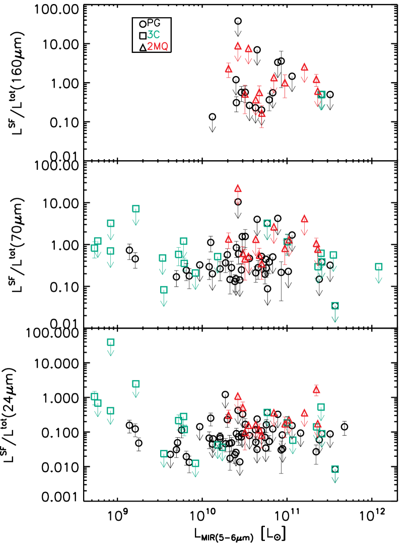
Figure 9.— The star-formation fraction at 24, 70 and 160 $\mu$m versus the mid-IR (5-6$\mu$m) luminosity for the PG, 3C and 2MASS objects, respectively (see the color version online).

Figure 10.— The star-formation fraction at 24, 70 and 160 $\mu$m versus the ratio of mid-IR (5-6 $\mu$m) luminosity and the Eddington luminosity for PG quasars. The solid line is the regression line and the two dotted lines are 2$\sigma$ confidence bounds.

Fig. 9 shows the star-formation contribution to the MIPS rest-frame 24, 70 and 160 $\mu$m emission versus the integrated mid-IR luminosity between 5.0 and 6.0 $\mu$m. The IRAS or ISO 25 $\mu$m fluxes are plotted for objects without MIPS 24 $\mu$m flux measurements. For objects without MIPS 70 $\mu$m flux measurements, we estimate one by interpolating between the detected IRAS or ISO 60 and 100 $\mu$m fluxes. The MIPS fluxes are K-corrected by assuming $\alpha$=1 for 24 and 70 $\mu$m photometry, and $\alpha$=0.0 for 160 $\mu$m photometry (f_ν $\propto$ $\nu^{-\alpha}$), based on the IR SED of AGN in Haas et al. (2003) and Shi et al. (2005). The total PAH-derived SFIR luminosities are converted to the star-formation emission at the three MIPS bands using the luminosity-dependent conversion factors derived from the star-forming templates from Dale et al. (2001) and Dale & Helou (2002).

At 24 $\mu$m, Fig. 9 indicates most of the objects are dominated by AGN emission. At 70 and 160 $\mu$m, the far-IR emission of an individual AGN can be dominated by either AGN power or star formation. To quantify the star-formation fraction at the three MIPS bands and its possible dependence on the AGN luminosity, we have employed the code written by Kelly (2007) that incorporates the upperlimit measurements. As listed in Table 2, the average star-formation fractions for the whole sample at MIPS 24, 70 and 160 $\mu$m are 4%, 26% and 28%, respectively, at the median mid-IR luminosity (2.6$\times$10¹⁰ L_⊙) of the sample. As indicated by Table 2, these ratios depend on luminosity, with a lower relative star-formation contribution at higher AGN mid-IR luminosity. The diverse nature of far-IR emission is consistent with the large scatter of the correlation between the far-IR emission and AGN power indicators (e.g. Shi et al., 2005; Cleary et al., 2006; Tadhunter et al., 2007). There will also be some scatter due to the range of redshifts. However, since the redshifts of our PG and 2MASS samples are similar and modest, the effect should be small.

Table 2 also includes the result for PG and 2MASS objects at the MIPS 24 and 70 $\mu$m bands, where there are enough detected data points. The average star-formation contributions at MIPS 70 $\mu$m for PG and 2MASS are 24% and 51% at median mid-IR luminosities of 3.0$\times$10¹⁰ L_⊙ and 3.5$\times$10¹⁰ L_⊙, respectively. The fraction for the PG quasars is lower than that ($>$30%) obtained by Schweitzer et al. (2006), who also employ the aromatic feature to evaluate the role of star formation. Contributions to the discrepancy include a difference in the conversion factors from the aromatic fluxes to the SFIR fluxes and the relatively large uncertainties in their 7.7 $\mu$m fluxes caused by silicate features, whereas our result is mainly based on 11.3 $\mu$m features.

Compared to the whole sample, PG objects show relatively stronger luminosity-dependence of the star-formation fractions at 24 and 70 $\mu$m, with decreasing fractions at higher mid-IR luminosities. However, the 2MASS objects do not have such a relation and most of the 3CR results are upperlimits. Thus the relation for the whole sample is mainly produced by the PG sample. As shown in Fig. 10 and Table 3, the star-formation fractions for the PG objects also decrease as the ratios of the mid-IR continuum luminosities and the Eddington luminosities decrease, where the blackhole masses of PG objects are obtained from Vestergaard & Peterson (2006) and Kaspi et al. (2000). The anti-correlations indicate these two relations are not caused by the selection effect that the detectable aromatic features in objects with higher mid-IR continuum emissions have larger fluxes.

6. STAR-FORMING IR LUMINOSITY FUNCTION OF QUASAR HOST GALAXIES

6.1. Methodology

The main challenge in deducing the SFIR luminosity function (LF) for our sample is that the flux limit of the aromatic feature is not well defined and many objects have only upper limits in these measurements. Therefore, we obtained the SFIR LF by converting the well-defined LF at other wavelengths using the fractional bivariate LF (Elvis et al., 1978). The formula can be written as

$$\Phi_{M_{\rm SFIR}}=\sum_{M_{\lambda}}\Phi_{M_{\lambda}}F(M_{\lambda},M_{\rm SFIR})$$ (2)

where $\Phi_{M_{\rm SFIR}}$ is the SFIR LF and $\Phi_{M_{\lambda}}$ is the LF at $\lambda$-band where each parent sample is selected (radio for 3CR objects, $B$-band for PG objects and $K$-band for 2MASS objects). The fractional bivariate LF $F(M_{\lambda},M_{\rm SFIR})$ indicates the fraction of objects with magnitude $M_{\lambda}$ at $\lambda$-band having SFIR luminosity of $M_{\rm SFIR}$. We calculate $F(M_{\lambda},M_{\rm SFIR})$${\Delta}M_{\lambda}$${\Delta}M_{\rm SFIR}$ by dividing the number $n_{1}$ of objects with $\lambda$-band magnitude in the interval $M_{\lambda}{\pm}{\Delta}M_{\lambda}/2$ and the SFIR luminosity in the interval $M_{\rm SFIR}{\pm}{\Delta}M_{\rm SFIR}/2$ by the number $n_{2}$ of objects with $\lambda$-band magnitude in the interval $M_{\lambda}{\pm}{\Delta}M_{\lambda}/2$ that could have had detected aromatic features if they had SFIR luminosities of $M_{\rm SFIR}$. $n_{1}$ is the observed number. Any object with $\lambda$-band magnitude in the interval $M_{\lambda}{\pm}{\Delta}M_{\lambda}/2$ will be counted into $n_{2}$, if it has a limiting SFIR luminosity lower than $M_{\rm SFIR}$. The limiting SFIR luminosity is defined as the minimum star formation rate to detect the aromatic feature (see § 2.3) plus any extended IR emission.

For PG quasars, $\Phi_{M_{\lambda}}$ is the $B$-band LF at 0.0$<z<$0.5 from Table 9 of Schmidt & Green (1983), where the median redshift of 0.25 is adopted to convert the apparent magnitude to the absolute magnitude and the K-correction is the same as described in Schmidt & Green (1983). This $B$-band LF has data coverage for $M_{B}$ from -21.4 mag to -26.4 mag. A double-exponential model (for the formula, see Le Floc’h et al., 2005) fits the $B$-band LF well and it is used to derive the $\Phi_{M_{B}}$ for any given $M_{B}$ between -21.0 and -26.5 for our PG subsample. The SFIR luminosity of this PG subsample spans the range from 3.1$\times 10^{9}$ to 2.4$\times 10^{12}$ L_⊙. To construct the fractional bivariate LF ($F$($M_{B}$, $M_{\rm SFIR}$)), the entire ranges of $M_{B}$ and SFIR luminosity are each divided into four intervals. The final fractional bivariate LF ($F$($M_{B}$, $M_{\rm SFIR}$)) along with Poissonian uncertainties is listed in Table 4.

For 2MASS objects, the LF at $K$ band from Cutri et al. (2001) is adopted as $\Phi_{M_{\lambda}}$. A two-exponential model does not fit the data well and thus we interpolate the measured data points to get the space density at a given $K$-band magnitude. Table 5 lists the final fractional bivariate LF ($F$($M_{B}$, $M_{\rm SFIR}$)) for 2MASS objects.

For 3CR objects, $\Phi_{M_{\lambda}}$ is the LF at 151 MHz from Willott et al. (2001), where the LF is obtained based on the 3CRR, 6CE and 7CRS samples. We use the analytic LF of model C for a cosmological model of $\Omega_{m}$=0, $\Omega_{\lambda}$=0 and $H_{0}$=50 kms^-1Mpc^-1, because the LF for this cosmological model is close to that for our cosmological model except for the $H_{0}$ value. (Willott et al., 2001). We convert to our cosmological model by setting $\Phi_{1}(L_{1},z)dV_{1}=\Phi_{2}(L_{2},z)dV_{2}$ (Peacock, 1985). The radio luminosity at 151 MHz for our 3CR subsample is calculated and K-corrected using the flux density and spectral index at 178 MHz from Spinrad et al. (1985). Again, we limit our 3CR subsample to the redshift range between 0.0 and 0.5 to match the PG and 2MASS redshift ranges. The final fractional bivariate LF ($F$($M_{151MHz}$, $M_{\rm SFIR}$)) with Poissonian uncertainties is listed in Table 6.

6.2. Star-forming IR Luminosity Function of Active Galaxies

6.2.1 Comparison to Field Galaxies

Figure 11.— Star-forming infrared luminosity functions for the PG, 2MASS and 3CR AGN. The dotted line is the re-normalized luminosity function of local field galaxies from Le Floc’h et al. (2005).

The most important result from the fractional bivariate LFs in Table 4, Table 5 and Table 6 is that objects with a large range of nuclear activity have a non-zero probability of having a high SFIR luminosity. The form of the fractional bivariate LF implies that SFIR LF of AGN host galaxies is much flatter than the LF of the AGN themselves.

Fig. 11 shows the results for the SFIR LF for the PG, 2MASS and 3CR subsamples. Each subsample has a brightness limit at the wavelength where it is selected. We set $M_{B}<$-21 for the PG subsample and $M_{K}<$-25.5 for the 2MASS subsample and $L_{\rm 151MHz}>$2$\times$10²⁴ W Hz^-1 Sr^-1 for the 3CR subsample. The dotted line shows the re-normalized IR LF of local field galaxies from Le Floc’h et al. (2005) based on the IRAS and ISO results; it agrees well with previous studies of the IR LF of field galaxies (See Rieke & Lebofsky, 1986; Sanders et al., 2003). In Fig. 11, the SFIR LFs of the three subsamples are much flatter than the re-normalized LFs of field galaxies.

We need to be sure that the flatter LFs are not just a result of the difficulty in measuring the SFR around a bright quasar. We first use Monte-Carlo simulations to test the robustness of the methodology used to derive the SFIR LF of AGNs. The following steps are taken to construct a sample that mimics the PG subsample: (1) a total of $N_{obj}$($>$10000) objects is created over the redshift range between 0.001 and 0.5; (2) the comoving number density is constant over the redshift range; (3) a $B$-band luminosity within the range of the PG subsample is assigned to each object randomly but the relative distribution is the same as the PG $B$-band LF; (4) similarly, each object has a randomly assigned IR luminosity with relative distribution defined by the SFIR LF of the PG subsample. In this case, the IR flux is not correlated with the $B$-band flux; (5) a well-defined flux limit is applied in the $B$-band while the IR flux limit is randomly distributed over the whole range of the SFIR fluxes of the PG subsample. After producing the above set of objects, the fractional bivariate LF is calculated based on those objects detected in the $B$-band. The final derived SFIR LF using the fractional bivariate LF follows the pre-defined SFIR LF within the Poission noise. The same result is obtained for the simulation in which the IR flux is tightly correlated with the $B$-band flux.

Unlike the PG subsample, which is complete, the 2MASS and 3CR subsamples only contain one-third of their parent samples at $z<$0.5. To test for the effects of the sample incompleteness, we use only one third of the objects brighter than the $B$-band limiting flux created in the above simulations, with these objects having the brightest apparent $B$-band magnitude. Again, the derived SFIR LF is consistent with pre-defined SFIR LF within the Poission noise. We also test using the one-third of the objects with the most luminous absolute $B$-band luminosity. The shape of the derived IR LF does not change but the normalization becomes smaller. The same result is obtained if the $B$-band flux correlates with the IR flux. Thus, for all three subsamples, the Monte Carlo code demonstrates the robustness of our methodology to derive the SFIR LF of AGNs

Because AGNs have strong mid-IR continua, aromatic features are detected only in host galaxies with intense star formation. We can now use the Monte-Carlo simulation to demonstrate that this selection effect cannot account for the large difference in the SFIR LF between the field galaxy and PG quasars. In the simulation, we assume the SFIR LF of PG quasars actually follows that of field galaxies. For each PG object, we obtain the IR LF of field galaxies at the redshift of this object by assuming that the local field galaxy IR LF from Le Floc’h et al. (2005) evolves with redshift as $L^{*}(z)=L^{*}(0)(1+z)^{3.2}$ and $\Phi^{*}(z)=\Phi^{*}(0)(1+z)^{0.7}$. We then randomly assign a SFIR luminosity to this PG object with a relative probability that follows the LF of field galaxies at this redshift. The range of the simulated SFIR luminosities is from 3.1$\times$10⁹ to 2.4$\times$10¹² L_⊙, consistent with the observed range for the PG quasars. Also, we assume that the total probability in this luminosity range is equal to 1. In this case, all simulated IR luminosities are above the low luminosity cut (3$\times$10⁹ L_⊙), and thus bias the results toward the high luminosity end. Combining the simulated SFIR luminosity and the observed uncertainty or upper limit for each PG object, we can calculate the detection fraction for the aromatic features. After one thousand simulations, we find (despite the bias toward high luminosity) that the detection fraction is only (28$\pm$3)%, much smaller than the observed value (48%). This large difference indicates that our result is not simply due to the selection toward high levels of SFR caused by the AGN emission.

We further measure the probability of producing the observed curvature of the SFIR LF if the PG quasar sample actually has a field galaxy SFIR LF. In each simulation, all PG objects are assigned randomly SFIR luminosities as described above. Using the simulated luminosities and the observed uncertainties or upperlimits, a SFIR LF is constructed using the same procedure including the number of luminosity bins as the observed LF. All data points produced in a total of ten thousand simulations are rebinned to the same bins as for the observed PG LF. In four luminosity bins, the fractions of simulated non-zero number densities are 100%, 100%, 64% and 6% from low to high luminosity. All simulated number densities are then rescaled by a factor to match the composite number density in the first luminosity bin to the observed one. This composite number density is assumed to be the median value of all simulated number densities (including zero value) in the first bin, indicating a probability of 50%. We then calculate the probability for an observed luminosity bin as the fraction of simulated number densities larger than the lower 1-sigma bound of the observed number density in this bin. The probability in each bin from low to high luminosity is 99.0%, 1.0%, 2.5% and 4.0%, respectively. This result provides further evidence that the flatter SFLF of the PG quasars is robust against selection effects.

6.2.2 Dependence on AGN Luminosity

Figure 12.— Star-forming infrared luminosity functions of PG quasars as a function of quasar brightness. The dashed line is the re-normalized luminosity function of star formation in CfA Seyfert 1 galaxies from Maiolino et al. (1995). The dotted line is the re-normalized luminosity function of local field galaxies from Le Floc’h et al. (2005). The solid lines are Schechter-function fits to the two PG subsamples.

Fig. 12 shows the SFIR LF of PG quasars as a function of the $B$-band luminosity. The two solid lines are Schechter-function fits for PG quasars at $M_{B}<$-21 and $M_{B}<$-23, respectively. The fitting parameters are given in Table 7. There is a trend that the SFIR LF of PG quasars becomes flatter for the brighter PG objects. We suggest that the higher SFR for brighter PG quasars is not a selection effect because the $B$-band luminosity of normal infrared galaxies is not well correlated with IR luminosity and LIRGs rarely have M_B $<$ -23 (See Rieke & Lebofsky, 1986). The trend seen in Fig. 12 is not likely to be due to evolution with redshift, as the mean redshifts for the faint and bright subsamples are nearly the same from faint to bright, 0.18$\pm$0.30 and 0.24$\pm$0.11 respectively.

In Fig. 12, the dashed line is the LF of extended star formation in CfA Seyfert 1 galaxies from Maiolino et al. (1995). The extended IR emission of Seyfert galaxies was obtained by subtracting the nuclear emission from IRAS 12 $\mu$m photometry (See Maiolino et al., 1995). We converted the 10 $\mu$m luminosity to the total IR luminosity using the IR SED template from Dale et al. (2001) and Dale & Helou (2002). Similarly to converting the aromatic flux to the total IR luminosity, the conversion factor from 10 $\mu$m to the total IR luminosity depends on the total IR luminosity. The omission of nuclear star formation (within 2^′′) in the study of Maiolino et al. (1995) may affect the LF of total star formation in their Seyfert galaxies. However, if nuclear star formation is correlated with the extended star formation as found by Buchanan et al. (2006), the shape of the LF for the total star formation in Seyfert galaxies should not change. As shown in Fig. 12, the SFIR LF of Seyfert 1 galaxies is steeper than the LF of PG quasars. There is also a suggestion that the LF for the lower-luminosity PG quasars is steeper than for the higher-luminosity ones. Seyfert galaxies have a higher SFR and flatter LF on average than field galaxies (see Fig. 12 and Maiolino et al., 1995). It appears that star formation is correlated with the level of nuclear activity over the full range from normal galaxies to quasars.

To test the trend of the SFIR LF of active galaxies as a function of AGN luminosity, we extended the Monte-Carlo simulations described in § 6.2.1 to test the difference between PG quasars with $M_{B}<$-21 and PG quasars with $M_{B}<$-23. In this simulation, we assume that the SFIR LF of PG quasars with $M_{B}<$-23 actually follows that of PG quasars with $M_{B}<$-21. For a PG quasar with $M_{B}<$-23, we obtain the SFIR LF of PG quasars with $M_{B}<$-21 at the redshift of this object by assuming the SFIR LF of PG quasars at $M_{B}<$-21 evolving with redshift as $L^{*}(z)=L^{*}(z_{1})(\frac{1+z}{1+z_{1}})^{3.2}$ and $\Phi^{*}(z)=\Phi^{*}(z_{1})(\frac{1+z}{1+z_{1}})^{0.7}$, where $z_{1}$ is the mean redshift (0.2) of PG quasars with $M_{B}<$-21. Based on this LF, a random SFIR luminosity is assigned to a PG quasar with $M_{B}<$-23. The luminosity range is between 3.1$\times$10⁹ and 2.4$\times$10¹², consistent with the observed range for PG quasars with $M_{B}<$-21. The total probability in this luminosity range is equal to 1. Using the observed uncertainties or upper limits, we predict the detection fraction of the aromatic feature for PG quasars at $M_{B}<$-23 of 17$\pm$5%, smaller than the observed fraction of 28%. This result supports our conclusion that the SFIR luminosity increases with increasing AGN luminosity.

6.2.3 Comparison Between Different Subsamples

As shown in Fig. 11, the behavior of star formation is different around AGN selected by different techniques. Since the SFIR LF of AGN host galaxies is a function of AGN luminosity as found in the last section, the effect of the nuclear brightness needs to be removed. The 2MASS $K$-band photometry for all PG objects was obtained from the 2MASS Point Source Catalog. We calculated $B-K$ for all PG objects and found that $<B-K>$=3.0$\pm$0.6 and is not a function of absolute $K$-band magnitude. All PG objects with $M_{B}<$-22.5 are selected to form a comparison sample for the 2MASS objects with $M_{K}<$-25.5. For the 3CR subsample, it is difficult to select a PG sample with the same level of nuclear activity. This is because PG objects are selected by thermal emission while 3CR objects are selected because of their non-thermal emission and there is no good correlation between the radio emission and the thermal mid-IR emission (Ogle et al., 2006). Instead, we compare the whole PG subsample at $M_{B}<$-21 to the whole 3CR subsample at $L_{151MHz}>$2$\times$10²⁴ W Hz^-1 Sr^-1.

Fig. 13 shows the cumulative fractional luminosity function F($>$L) = $\sum_{L=L_{0}}^{\infty}$ f(L) for PG versus 2MASS and PG versus 3CR. To avoid biases due to evolution, the comparison includes objects with $z<$0.5. The fractional luminosity function f(L) is defined similarly to the fractional bivariate LF (See Elvis et al., 1978; Golombek et al., 1988). As shown in Fig. 13, there is an apparent sequence in terms of the level of SFR that progresses from 3CR to PG to 2MASS objects that generally show the highest SFRs. The median star-forming IR luminosities of 3CR, PG and 2MASS objects are 6$\times$10⁹, 3.0$\times 10^{10}$ and 1$\times$10¹¹ L_⊙, respectively. Different AGN selection techniques appear to identify objects with different levels of star forming activity in their host galaxies.

Figure 13.— Cumulative fraction luminosity functions F($>$L) = $\sum_{L=L_{0}}^{\infty}$ f(L) for the PG objects versus 2MASS objects (upper plot) and the PG objects versus 3CR objects (lower plot), where f(L) is the fractional luminosity function (See text).

6.3. Implications for Nuclear Activity

The flatter SFIR LF of AGN host galaxies indicates enhanced star-forming activity relative to local field galaxies. Previous studies illustrate the presence of significant post-starburst stellar populations in quasar host galaxies. For example, the optical and near-IR broadband SEDs of AGN indicate the presence of young stellar populations with an age of about a Gyr in the host galaxies, independent of morphological type (Jahnke et al., 2004), consistent with previous studies (Kotilainen & Ward, 1994; Schade et al., 2000; Ronnback et al., 1996). In addition, Kauffmann et al. (2003) found a trend of younger mean stellar population for higher-luminosity AGN based on a very large sample. None of these studies found evidence for intense on-going massive star formation, except for a few objects (see Jahnke et al., 2004). We emphasize that the techniques employed in the above studies are unable to detect OB stars or suffer from strong degeneracy between the current star-formation and the star-formation history. Therefore, these studies do not contradict our result. Searches for massive star formation through UV spectroscopy or spatially-resolved observations for star-formation tracers (such as recombination lines and IR emission) indicate the presence of massive star formation in Seyfert galaxies (Maiolino et al., 1995; Heckman et al., 1997) and in quasars (Cresci et al., 2004). All of these studies focus on the central region of the galaxy, implying that the star formation in quasars is circumnuclear. This is consistent with the lack of spectroscopic evidence for on-going star formation at distances from the nuclei of $\sim$15 kpc (Nolan et al., 2001).

The flatter SFIR LF of AGN host galaxies relative to field galaxies also implies that nuclear activity tends to be triggered in galaxies with enhanced star formation. Based on Fig. 11, we can calculate the probability of triggering a PG quasar in field galaxies at a given SFR; for example, the probability of triggering nuclear activity at $L_{SFIR}$=1.25$\times$10¹² L_⊙ is a factor of 50 higher than that at $L_{SFIR}$=1$\times$10¹⁰ L_⊙. This indicates an environment with intense star formation offers preferential conditions for nuclear activity, such as the abundant inflowing material driven by star formation (Granato et al., 2004). On the other hand, it implies that over much of the life of an AGN, its feedback does not quench the star formation, but instead may enhance the host galaxy star formation as demonstrated in some numerical simulations (Silk, 2005). Our result that more luminous AGNs are more likely to reside in host galaxies with more intense star formation provides further evidence that feedback from the two physical processes (star formation and nuclear activity) can enhance both processes. Numerical simulations have predicted the evolution of the SFR and SMBH accretion rate along the merging process (Granato et al., 2004; Springel et al., 2005). They conclude that the evolution of star formation almost follows the SMBH accretion rate, although the former starts to decline a little earlier. A more quantative and careful comparison between the simulations and our observations will improve our understanding of when and how feedback plays a role in galaxy evolution and SMBH growth.

Although PG, 2MASS and 3CR AGN have flatter SFIR LFs compared to field galaxies, they show differences in the distribution of SFRs, as indicated by the cumulative fractional LFs in Fig. 13. Fig. 8 shows that the SFR of AGN host galaxies correlates with the amount of molecular gas in the host galaxy, which suggests that different AGN selection methods prefer host galaxies with different levels of gas reservoir. It is interesting that PG and 2MASS quasars have different levels of SFR. Both samples are selected through thermal emission. There is no obscuration along the line of sight for PG objects while the red IR-optical color of 2MASS objects is attributed to the obscuration of nuclear radiation by dust in the circumnuclear regions or host galaxies (e.g. Smith et al., 2002; Marble et al., 2003). According to the AGN unification model (Antonucci, 1993), 2MASS objects are reddened counterparts of PG objects. The different levels of star formation in 2MASS and PG objects suggest that star formation affects our view of the AGN phenomenon, which is not expected under the unification model. This is not a selection effect that 2MASS objects need to have a larger SFR to have comparable the $K$-band luminosity to PG quasars, as $K$-band fluxes in 2MASS objects are dominated by hot dust or starlight, not by star formation. A similar correlation has been observed in Seyfert galaxies, that Seyfert 2 objects have larger star formation rates than Seyfert 1s (e.g. Edelson et al., 1987; Maiolino et al., 1995). Observations and numerical simulations show that the feedback produced by nuclear star formation can heat the circumnuclear material and thus increase its scale height (Maiolino et al., 1999; Ohsuga & Umemura, 1999; Wada & Norman, 2002; Watabe & Umemura, 2005). Such behavior could produce the link between star formation activity and AGN properties.

7. CONCLUSIONS

We present Spitzer IRS observations of three AGN samples including PG quasars, 2MASS quasars and 3CR radio-loud AGNs. The PG sample includes all PG quasars at z$<$0.5 while one third of the 2MASS and 3CR parent samples are used in this study. The main results are the following:

1. The aromatic features at 7.7 and 11.3 $\mu$m are detected against the strong mid-IR continuum of the AGN. The excitation mechanism for the aromatic features is predominantly star formation.

2. The contribution of star formation to the far-IR emission of individual AGN is diverse; the average contribution is around 25% at 70 and 160 $\mu$m. For the PG objects, this contribution shows anti-correlations with the mid-IR luminosity and the ratio of the mid-IR continuum and the Eddington luminosity.

3. The star-forming IR luminosity functions of AGNs are flatter than that of field galaxies, implying the feedback from star formation and nuclear activity can enhance both processes.

4. The star-forming IR luminosity function of AGNs is correlated with the level of nuclear activity over the whole range from normal galaxies to bright quasars, with higher star formation rates for more intense nuclear activity. The 2MASS, PG and 3CR AGNs have distributions of star formation that follow the progression (from high to low SFR) of 2MASS-PG-3CR, implying that various AGN survey techniques select host galaxies with different levels of star forming activity.

Table 1 AGN with associated physical parameters

source	Redshift	F(7.7$\mu$m)	EW(7.7$\mu$m)	F(11.3$\mu$m)	EW(11.3$\mu$m)	$L_{\rm SFIR}$	$L_{5-6{\mu}m}$	S${}_{\rm CO}{\Delta}V$	Ref
(1)	(2)	(3)	(4)	(5)	(6)	(7)	(8)	(9)	(10)
PG0003+158	0.450			$<$ 0.13			1.2${\times}10^{11}$
PG0003+199	0.025	$<$ 1.39		0.29$\pm$0.06	0.01	(8.8$\pm$4.03)${\times}10^{08}$	3.3${\times}10^{09}$
PG0007+106	0.089	$<$ 1.39		0.51$\pm$0.06	0.03	(3.2$\pm$1.32)${\times}10^{10}$	1.9${\times}10^{10}$	$<$ 3.00	1
PG0026+129	0.142	$<$ 0.36		$<$ 0.12		$<$4.5${\times}10^{10}$	3.0${\times}10^{10}$
PG0043+039	0.385	$<$ 0.36		$<$ 0.08		$<$5.1${\times}10^{11}$	1.0${\times}10^{11}$
PG0049+171	0.064	$<$ 0.50		$<$ 0.05		$<$3.1${\times}10^{09}$	2.1${\times}10^{09}$
PG0050+124	0.061	8.28$\pm$5.61	0.05	2.77$\pm$0.25	0.02	(9.3$\pm$3.82)${\times}10^{10}$	4.3${\times}10^{10}$	18.00	2
PG0052+251	0.155	$<$ 1.74		0.55$\pm$0.12	0.05	(1.3$\pm$0.62)${\times}10^{11}$	3.2${\times}10^{10}$	2.00	3
PG0157+001	0.163	6.71$\pm$2.44	0.25	2.44$\pm$0.16	0.09	(8.9$\pm$3.61)${\times}10^{11}$	5.7${\times}10^{10}$	8.10
PG0804+761	0.100	$<$ 1.75		$<$ 0.19		$<$3.8${\times}10^{10}$	5.6${\times}10^{10}$	2.00	2
PG0838+770	0.131	1.46$\pm$0.60	0.17	$<$ 0.23		(6.1$\pm$3.09)${\times}10^{10}$	1.2${\times}10^{10}$	3.40	1
PG0844+349	0.064	1.56$\pm$0.60	0.09	0.38$\pm$0.07	0.03	(1.0$\pm$0.44)${\times}10^{10}$	6.5${\times}10^{09}$	$<$ 1.50	2
PG0921+525	0.035	$<$ 0.59		$<$ 0.05		$<$8.6${\times}10^{08}$	2.2${\times}10^{09}$
PG0923+201	0.190	$<$ 0.35		$<$ 0.29		$<$9.0${\times}10^{10}$	5.9${\times}10^{10}$
PG0923+129	0.029	9.73$\pm$2.28	0.28	2.42$\pm$0.13	0.08	(1.3$\pm$0.51)${\times}10^{10}$	1.6${\times}10^{09}$
PG0934+013	0.050	2.86$\pm$0.60	0.26	0.74$\pm$0.05	0.08	(1.2$\pm$0.48)${\times}10^{10}$	1.8${\times}10^{09}$
PG0946+301	1.216	$<$ 0.47		$<$ 0.11		$<$1.8${\times}10^{13}$	1.7${\times}10^{12}$
PG0947+396	0.205	$<$ 0.38		$<$ 0.18		$<$1.2${\times}10^{11}$	5.0${\times}10^{10}$
PG0953+414	0.234	$<$ 1.39		$<$ 0.20		$<$3.8${\times}10^{11}$	7.8${\times}10^{10}$
PG1001+054	0.160	$<$ 0.38		0.17$\pm$0.03	0.03	(3.8$\pm$1.66)${\times}10^{10}$	2.7${\times}10^{10}$
PG1004+130	0.240	$<$ 0.58		0.20$\pm$0.05	0.02	(1.3$\pm$0.62)${\times}10^{11}$	6.2${\times}10^{10}$
PG1011-040	0.058	$<$ 0.56		0.50$\pm$0.04	0.03	(1.1$\pm$0.44)${\times}10^{10}$	3.6${\times}10^{09}$
PG1012+008	0.186	$<$ 0.61		$<$ 0.09		$<$8.2${\times}10^{10}$	3.6${\times}10^{10}$
PG1022+519	0.044	4.22$\pm$0.74	0.44	1.32$\pm$0.08	0.19	(1.8$\pm$0.73)${\times}10^{10}$	1.4${\times}10^{09}$
PG1048+342	0.167	$<$ 0.33		$<$ 0.04		$<$2.1${\times}10^{10}$	1.3${\times}10^{10}$
PG1048-090	0.344	$<$ 0.33		$<$ 0.06		$<$2.8${\times}10^{11}$	5.4${\times}10^{10}$
PG1049-005	0.359	1.17$\pm$0.38	0.07	0.17$\pm$0.07	0.01	(3.4$\pm$1.93)${\times}10^{11}$	2.2${\times}10^{11}$
PG1100+772	0.311	$<$ 1.04		0.29$\pm$0.08	0.04	(4.1$\pm$1.99)${\times}10^{11}$	1.0${\times}10^{11}$
PG1103-006	0.423	$<$ 0.18		$<$ 0.09		$<$3.6${\times}10^{11}$	1.3${\times}10^{11}$
PG1114+445	0.143	$<$ 0.40		$<$ 0.11		$<$5.2${\times}10^{10}$	4.4${\times}10^{10}$
PG1115+407	0.154	2.55$\pm$0.33	0.28	0.46$\pm$0.03	0.08	(1.1$\pm$0.46)${\times}10^{11}$	2.1${\times}10^{10}$
PG1116+215	0.176	$<$ 3.32		$<$ 0.25		$<$2.3${\times}10^{11}$	1.1${\times}10^{11}$
PG1119+120	0.050	2.26$\pm$0.89	0.06	0.80$\pm$0.09	0.03	(1.3$\pm$0.53)${\times}10^{10}$	5.0${\times}10^{09}$	4.50	1
PG1121+422	0.225	$<$ 0.35		$<$ 0.09		$<$1.2${\times}10^{11}$	3.0${\times}10^{10}$
PG1126-041	0.060	$<$ 1.23		1.35$\pm$0.36	0.04	(3.6$\pm$1.75)${\times}10^{10}$	1.6${\times}10^{10}$	$<$ 2.60	1
PG1149-110	0.049	$<$ 0.64		$<$ 0.10		$<$3.5${\times}10^{09}$	2.2${\times}10^{09}$
PG1151+117	0.176	$<$ 3.30		$<$ 0.48		$<$5.2${\times}10^{11}$	1.9${\times}10^{10}$
PG1202+281	0.165	1.41$\pm$0.48	0.14	0.37$\pm$0.05	0.04	(1.0$\pm$0.44)${\times}10^{11}$	2.5${\times}10^{10}$	$<$ 2.40	1
PG1211+143	0.080	$<$ 1.82		$<$ 0.15		$<$1.9${\times}10^{10}$	2.8${\times}10^{10}$	$<$ 1.50	2
PG1216+069	0.331	$<$ 0.34		$<$ 0.05		$<$1.9${\times}10^{11}$	8.9${\times}10^{10}$
PG1226+023	0.158	$<$ 2.16		$<$ 0.16		$<$1.0${\times}10^{11}$	3.7${\times}10^{11}$
PG1229+204	0.063	$<$ 0.54		0.38$\pm$0.12	0.02	(9.8$\pm$4.94)${\times}10^{09}$	7.0${\times}10^{09}$	2.40	2
PG1244+026	0.048	1.76$\pm$0.86	0.14	0.51$\pm$0.04	0.04	(7.0$\pm$2.86)${\times}10^{09}$	1.8${\times}10^{09}$
PG1259+593	0.477	$<$ 0.16		$<$ 0.04		$<$3.8${\times}10^{11}$	2.7${\times}10^{11}$
PG1302-102	0.278	$<$ 0.51		$<$ 0.14		$<$3.7${\times}10^{11}$	1.0${\times}10^{11}$
PG1307+085	0.155	$<$ 3.47		$<$ 0.43		$<$3.2${\times}10^{11}$	2.6${\times}10^{10}$
PG1309+355	0.184	$<$ 3.17		$<$ 0.36		$<$3.9${\times}10^{11}$	4.4${\times}10^{10}$	$<$ 0.61	3
PG1310-108	0.034	2.40$\pm$0.86	0.11	0.18$\pm$0.03	0.01	(1.0$\pm$0.44)${\times}10^{09}$	1.3${\times}10^{09}$
PG1322+659	0.168	0.72$\pm$0.30	0.07	0.20$\pm$0.02	0.03	(5.3$\pm$2.20)${\times}10^{10}$	2.9${\times}10^{10}$
PG1341+258	0.087	0.45$\pm$0.21	0.06	0.11$\pm$0.02	0.02	(5.3$\pm$2.39)${\times}10^{09}$	4.7${\times}10^{09}$
PG1351+236	0.055	7.54$\pm$1.05	0.87	2.75$\pm$0.12	0.44	(6.7$\pm$2.71)${\times}10^{10}$	1.6${\times}10^{09}$
PG1351+640	0.088	3.12$\pm$6.54	0.09	1.29$\pm$0.15	0.03	(9.3$\pm$3.89)${\times}10^{10}$	2.2${\times}10^{10}$	4.00	2
PG1352+183	0.152	$<$14.14		$<$ 2.60		$<$2.4${\times}10^{12}$	1.7${\times}10^{10}$
PG1354+213	0.300	$<$ 0.27		$<$ 0.06		$<$1.8${\times}10^{11}$	4.2${\times}10^{10}$
PG1402+261	0.164	$<$ 1.59		$<$ 0.22		$<$1.6${\times}10^{11}$	6.8${\times}10^{10}$	$<$ 2.00	1
PG1404+226	0.098	0.88$\pm$0.37	0.14	0.25$\pm$0.02	0.05	(1.7$\pm$0.71)${\times}10^{10}$	5.1${\times}10^{09}$		2
PG1411+442	0.089			0.31$\pm$0.04	0.01	(1.8$\pm$0.74)${\times}10^{10}$		$<$ 1.80	2
PG1415+451	0.113	1.67$\pm$0.30	0.14	0.86$\pm$0.06	0.10	(1.1$\pm$0.43)${\times}10^{11}$	1.3${\times}10^{10}$	3.30	1
PG1416-129	0.129	$<$ 0.56		$<$ 0.15		$<$5.8${\times}10^{10}$	8.5${\times}10^{09}$
PG1425+267	0.366	$<$ 0.45		$<$ 0.06		$<$3.1${\times}10^{11}$	1.1${\times}10^{11}$
PG1426+015	0.086	1.19$\pm$0.64	0.03	0.31$\pm$0.06	0.01	(1.7$\pm$0.73)${\times}10^{10}$	2.4${\times}10^{10}$	3.60	2
PG1427+480	0.221	$<$ 0.28		$<$ 0.03		$<$3.4${\times}10^{10}$	2.5${\times}10^{10}$
PG1435-067	0.126	$<$ 0.44		$<$ 0.19		$<$4.3${\times}10^{10}$	1.7${\times}10^{10}$
PG1440+356	0.079	6.74$\pm$2.89	0.20	2.27$\pm$0.13	0.10	(1.3$\pm$0.53)${\times}10^{11}$	2.0${\times}10^{10}$	9.00	2
PG1444+407	0.267	0.38$\pm$0.28	0.03	$<$ 0.15		(7.8$\pm$6.19)${\times}10^{10}$	8.5${\times}10^{10}$	0.71	3
PG1448+273	0.065	1.98$\pm$0.59	0.11	0.94$\pm$0.06	0.07	(3.0$\pm$1.22)${\times}10^{10}$	5.7${\times}10^{09}$
PG1501+106	0.036	$<$ 1.70		$<$ 0.38		$<$7.9${\times}10^{09}$	4.2${\times}10^{09}$
PG1512+370	0.370	$<$ 0.22		$<$ 0.07		$<$3.1${\times}10^{11}$	8.8${\times}10^{10}$
PG1519+226	0.137	0.59$\pm$0.21	0.04	0.21$\pm$0.02	0.02	(3.3$\pm$1.37)${\times}10^{10}$	2.7${\times}10^{10}$
PG1534+580	0.029	1.45$\pm$0.72	0.05	0.44$\pm$0.08	0.02	(2.0$\pm$0.88)${\times}10^{09}$	1.5${\times}10^{09}$
PG1535+547	0.038	0.62$\pm$0.22	0.02	0.08$\pm$0.03	0.01	(5.6$\pm$2.87)${\times}10^{08}$	3.1${\times}10^{09}$
PG1543+489	0.399	$<$ 0.34		$<$ 0.26		$<$6.3${\times}10^{11}$	2.4${\times}10^{11}$
PG1545+210	0.264	$<$ 1.75		$<$ 0.17		$<$4.1${\times}10^{11}$	5.8${\times}10^{10}$	$<$ 0.96	3
PG1552+085	0.119	$<$ 0.30		0.11$\pm$0.02	0.02	(1.1$\pm$0.46)${\times}10^{10}$	1.0${\times}10^{10}$
PG1612+261	0.130	$<$ 0.46		0.38$\pm$0.22	0.03	(5.8$\pm$4.17)${\times}10^{10}$	2.1${\times}10^{10}$
PG1613+658	0.129	3.02$\pm$1.87	0.08	0.77$\pm$0.09	0.03	(1.3$\pm$0.53)${\times}10^{11}$	5.5${\times}10^{10}$	8.50	1
PG1617+175	0.112	$<$ 0.45		$<$ 0.48		$<$3.2${\times}10^{10}$	1.9${\times}10^{10}$
PG1626+554	0.133	$<$ 0.47		$<$ 0.09		$<$3.2${\times}10^{10}$	1.3${\times}10^{10}$
PG1634+706	1.334	$<$ 0.52		$<$ 0.11		$<$2.4${\times}10^{13}$	9.4${\times}10^{09}$
PG1700+518	0.292	$<$ 5.70		$<$ 0.20		$<$6.5${\times}10^{11}$	3.2${\times}10^{11}$
PG1704+608	0.371	$<$ 1.04		$<$ 0.11		$<$6.5${\times}10^{11}$	2.6${\times}10^{11}$
PG2112+059	0.466	$<$ 0.24		0.27$\pm$0.05	0.02	(1.2$\pm$0.52)${\times}10^{12}$	4.8${\times}10^{11}$
PG2130+099	0.062	4.20$\pm$1.29	0.06	0.55$\pm$0.21	0.01	(1.5$\pm$0.83)${\times}10^{10}$	2.1${\times}10^{10}$	4.30	2
PG2209+184	0.070	1.32$\pm$0.37	0.20	0.29$\pm$0.03	0.06	(9.1$\pm$3.74)${\times}10^{09}$	3.0${\times}10^{09}$
PG2214+139	0.065	$<$ 0.81		$<$ 0.28		$<$1.7${\times}10^{10}$	1.6${\times}10^{10}$	1.60	2
PG2233+134	0.325	$<$ 1.44		$<$ 0.15		$<$6.6${\times}10^{11}$	9.4${\times}10^{10}$
PG2251+113	0.325	$<$ 0.55		$<$ 0.26		$<$6.3${\times}10^{11}$	1.5${\times}10^{11}$
PG2304+042	0.042	$<$ 0.46		$<$ 0.05		$<$5.6${\times}10^{09}$	8.8${\times}10^{08}$
PG2308+098	0.433	$<$ 0.27		$<$ 0.06		$<$5.4${\times}10^{11}$	1.4${\times}10^{11}$
PG2349-014	0.174	$<$ 0.47		0.41$\pm$0.10	0.05	(1.3$\pm$0.61)${\times}10^{11}$	4.6${\times}10^{10}$	3.20	3
2MASSJ000703.61+155423.8	0.114	3.00$\pm$0.71	0.32	1.00$\pm$0.10	0.14	(1.3$\pm$0.52)${\times}10^{11}$	9.7${\times}10^{09}$
2MASSJ005055.70+293328.1	0.136	1.76$\pm$0.34	0.19	0.33$\pm$0.09	0.05	(5.6$\pm$2.71)${\times}10^{10}$	1.5${\times}10^{10}$
2MASSJ010835.16+214818.6	0.285	$<$ 1.25		$<$ 0.21		$<$6.6${\times}10^{11}$	1.1${\times}10^{11}$
2MASSJ015721.05+171248.4	0.213	2.02$\pm$0.46	0.33	0.58$\pm$0.12	0.16	(3.5$\pm$1.56)${\times}10^{11}$	3.0${\times}10^{10}$
2MASSJ022150.60+132741.0	0.140	$<$ 3.31		$<$ 0.39		$<$2.1${\times}10^{11}$	2.5${\times}10^{10}$
2MASSJ023430.64+243835.5	0.310	$<$ 1.16		$<$ 0.34		$<$1.3${\times}10^{12}$	6.4${\times}10^{10}$
2MASSJ034857.64+125547.3	0.210	$<$ 1.56		$<$ 0.33		$<$5.2${\times}10^{11}$	2.3${\times}10^{11}$
2MASSJ091848.63+211717.1	0.149	$<$ 1.27		0.45$\pm$0.25	0.04	(1.0$\pm$0.69)${\times}10^{11}$	3.2${\times}10^{10}$
2MASSJ095504.56+170556.1	0.139	$<$ 1.10		$<$ 0.28		$<$1.4${\times}10^{11}$	9.5${\times}10^{09}$
2MASSJ102724.95+121920.4	0.231	$<$ 1.49		$<$ 0.36		$<$7.1${\times}10^{11}$	7.0${\times}10^{10}$
2MASSJ105144.25+353930.7	0.158	$<$ 0.99		$<$ 0.24		$<$1.7${\times}10^{11}$	1.0${\times}10^{10}$
2MASSJ125807.46+232921.5	0.259	1.54$\pm$0.78	0.09	$<$ 0.16		(3.9$\pm$2.29)${\times}10^{11}$	9.4${\times}10^{10}$
2MASSJ130005.35+163214.8	0.080	$<$ 4.82		$<$ 1.05		$<$1.7${\times}10^{11}$	2.2${\times}10^{10}$
2MASSJ130700.66+233805.0	0.275	9.27$\pm$1.58	0.57	$<$ 0.27		(3.9$\pm$1.33)${\times}10^{12}$	2.2${\times}10^{11}$
2MASSJ140251.22+263117.5	0.187	$<$ 1.46		$<$ 0.58		$<$4.4${\times}10^{11}$	2.6${\times}10^{10}$
2MASSJ145331.51+135358.7	0.139	10.31$\pm$2.81	0.51	1.10$\pm$0.70	0.16	(2.3$\pm$1.76)${\times}10^{11}$	4.0${\times}10^{10}$
2MASSJ150113.21+232908.3	0.258	$<$ 1.31		0.19$\pm$0.08	0.03	(1.4$\pm$0.82)${\times}10^{11}$	5.0${\times}10^{10}$
2MASSJ151653.24+190048.4	0.190	$<$ 2.22		$<$ 0.57		$<$7.2${\times}10^{11}$	1.6${\times}10^{11}$
2MASSJ163700.22+222114.0	0.211	2.81$\pm$0.61	0.60	0.51$\pm$0.04	0.15	(2.7$\pm$1.10)${\times}10^{11}$	2.0${\times}10^{10}$
2MASSJ165939.77+183436.9	0.170	3.43$\pm$1.21	0.17	0.65$\pm$0.16	0.04	(2.2$\pm$1.01)${\times}10^{11}$	4.7${\times}10^{10}$
2MASSJ171442.77+260248.5	0.163	1.19$\pm$0.34	0.20	0.32$\pm$0.07	0.08	(8.0$\pm$3.60)${\times}10^{10}$	1.7${\times}10^{10}$
2MASSJ222202.22+195231.5	0.366	$<$ 0.97		$<$ 0.09		$<$5.0${\times}10^{11}$	2.7${\times}10^{11}$
2MASSJ222221.12+195947.4	0.211	$<$ 1.05		$<$ 0.14		$<$1.8${\times}10^{11}$	4.3${\times}10^{10}$
2MASSJ222554.27+195837.0	0.147	1.97$\pm$0.33	0.22	$<$ 0.21		(1.2$\pm$0.40)${\times}10^{11}$	1.6${\times}10^{10}$
2MASSJ234449.57+122143.4	0.199	$<$ 1.25		$<$ 0.15		$<$1.8${\times}10^{11}$	3.5${\times}10^{10}$
3C6.1	0.840			$<$ 0.05		$<$2.5${\times}10^{12}$
3C15	0.073	$<$ 0.52		$<$ 0.03		$<$2.4${\times}10^{09}$	1.0${\times}10^{09}$
3C20	0.174	$<$ 1.20		$<$ 0.24		$<$2.1${\times}10^{11}$	4.2${\times}10^{09}$
3C22	0.936			$<$ 0.03		$<$1.5${\times}10^{12}$
3C28	0.195	$<$ 0.30		$<$ 0.06		$<$5.3${\times}10^{10}$	8.6${\times}10^{08}$
3C29	0.045	$<$ 0.75		$<$ 0.02		$<$6.6${\times}10^{08}$	2.3${\times}10^{08}$
3C33	0.059	$<$ 0.60		$<$ 0.15		$<$9.1${\times}10^{09}$	2.7${\times}10^{09}$
3C33.1	0.180	$<$ 1.62		$<$ 0.39		$<$4.0${\times}10^{11}$	1.2${\times}10^{10}$
3C47	0.425	$<$ 0.28		$<$ 0.06		$<$4.1${\times}10^{11}$	1.1${\times}10^{11}$
3C48	0.367	$<$ 4.55		$<$ 0.53		$<$4.0${\times}10^{12}$	2.5${\times}10^{11}$	2.00	4
3C55	0.734	$<$ 0.18		$<$ 0.07		$<$1.7${\times}10^{12}$	8.9${\times}10^{10}$
3C61.1	0.187	$<$ 0.23		$<$ 0.05		$<$4.2${\times}10^{10}$	8.3${\times}10^{08}$
3C65	1.176	$<$ 0.42		$<$ 0.08		$<$1.2${\times}10^{13}$	8.1${\times}10^{09}$
3C75	0.023	$<$ 0.33		$<$ 0.01		$<$7.6${\times}10^{07}$	2.6${\times}10^{07}$
3C76.1	0.032	$<$ 0.43		$<$ 0.05		$<$6.3${\times}10^{08}$	9.4${\times}10^{07}$
3C79	0.255	$<$ 1.02		$<$ 0.17		$<$3.9${\times}10^{11}$	3.0${\times}10^{10}$
3C83.1	0.025	$<$ 0.36		0.16$\pm$0.02	0.09	(4.4$\pm$1.84)${\times}10^{08}$	4.6${\times}10^{08}$
3C84	0.017			4.11$\pm$1.19	0.02	(7.1$\pm$3.53)${\times}10^{09}$	1.6${\times}10^{09}$
3C109	0.305	$<$ 1.75		$<$ 0.26		$<$1.1${\times}10^{12}$	2.2${\times}10^{11}$
3C123	0.217	$<$ 0.61		$<$ 0.05		$<$5.6${\times}10^{10}$	1.3${\times}10^{09}$
3C129	0.020	$<$ 0.36		0.07$\pm$0.01	0.06	(1.3$\pm$0.56)${\times}10^{08}$	1.2${\times}10^{08}$
3C138	0.759			$<$ 0.03		$<$1.0${\times}10^{12}$
3C147	0.545			$<$ 0.05		$<$6.6${\times}10^{11}$
3C153	0.276	$<$ 0.40		$<$ 0.04		$<$8.2${\times}10^{10}$	4.7${\times}10^{08}$
3C172	0.519	$<$ 0.17		$<$ 0.05		$<$5.8${\times}10^{11}$	5.5${\times}10^{09}$
3C173.1	0.292	$<$ 0.31		$<$ 0.03		$<$6.6${\times}10^{10}$	1.6${\times}10^{09}$
3C175	0.770	$<$ 0.17		$<$ 0.03		$<$1.0${\times}10^{12}$	2.8${\times}10^{11}$
3C184	0.994			$<$ 0.06		$<$5.7${\times}10^{12}$
3C192	0.059	$<$ 0.43		$<$ 0.05		$<$2.8${\times}10^{09}$	2.1${\times}10^{08}$
3C196	0.871	$<$ 0.14		$<$ 0.04		$<$2.1${\times}10^{12}$	3.3${\times}10^{11}$
3C200	0.458			$<$ 0.09		$<$9.4${\times}10^{11}$
3C216	0.670	$<$ 0.28		$<$ 0.12		$<$2.3${\times}10^{12}$	2.5${\times}10^{11}$
3C219	0.174	$<$ 0.30		$<$ 0.10		$<$5.9${\times}10^{10}$	6.0${\times}10^{09}$
3C220.1	0.610	$<$ 0.29		$<$ 0.10		$<$1.8${\times}10^{12}$	1.7${\times}10^{10}$
3C220.3	0.680	$<$ 1.05		$<$ 0.03		$<$6.9${\times}10^{11}$	1.6${\times}10^{10}$
3C234	0.184	$<$ 0.90		$<$ 0.24		$<$2.4${\times}10^{11}$	1.2${\times}10^{11}$
3C244.1	0.428	$<$ 0.21		$<$ 0.04		$<$3.3${\times}10^{11}$	2.5${\times}10^{10}$
3C249.1	0.311	$<$ 1.04		0.29$\pm$0.10	0.04	(4.1$\pm$2.16)${\times}10^{11}$	1.0${\times}10^{11}$
3C263	0.646	$<$ 0.14		$<$ 0.07		$<$9.4${\times}10^{11}$	3.6${\times}10^{11}$
3C263.1	0.824	$<$ 0.10		$<$ 0.16		$<$1.2${\times}10^{12}$	1.6${\times}10^{10}$
3C265	0.811	0.62$\pm$0.23	0.24	$<$ 0.30		(3.4$\pm$1.62)${\times}10^{12}$	2.6${\times}10^{11}$
3C268.1	0.970	$<$ 0.15		$<$ 0.08		$<$3.2${\times}10^{12}$	2.2${\times}10^{10}$
3C270	0.007			0.60$\pm$0.04	0.09	(1.4$\pm$0.56)${\times}10^{08}$	5.4${\times}10^{07}$
3C272	0.944			$<$ 0.02		$<$1.1${\times}10^{12}$
3C272.1	0.003			1.70$\pm$0.12	0.33	(2.0$\pm$0.04)${\times}10^{09}$	3.0${\times}10^{07}$
3C273	0.158	$<$ 2.16		$<$ 0.16		$<$1.0${\times}10^{11}$	3.7${\times}10^{11}$
3C274	0.004			$<$ 0.97		$<$2.3${\times}10^{08}$	4.3${\times}10^{07}$	$<$ 11.7	5
3C274.1	0.422	$<$ 0.19		$<$ 0.08		$<$3.7${\times}10^{11}$	3.0${\times}10^{09}$
3C275.1	0.555	$<$ 0.15		0.09$\pm$0.02	0.09	(5.1$\pm$2.29)${\times}10^{11}$	5.2${\times}10^{10}$
3C280	0.996	$<$ 0.09		$<$ 0.09		$<$1.9${\times}10^{12}$	2.3${\times}10^{11}$
3C292	0.710			$<$ 0.09		$<$3.4${\times}10^{12}$
3C293	0.045	3.96$\pm$0.70	0.62	1.27$\pm$0.10	0.41	(1.7$\pm$0.71)${\times}10^{10}$	9.2${\times}10^{08}$
3C295	0.464	$<$ 0.13		$<$ 0.24		$<$3.1${\times}10^{11}$	3.5${\times}10^{09}$
3C298	1.436	$<$ 0.30		$<$ 0.07		$<$1.7${\times}10^{13}$	1.2${\times}10^{12}$
3C300	0.270	$<$ 0.34		$<$ 0.06		$<$1.2${\times}10^{11}$	1.5${\times}10^{09}$
3C303.1	0.267	$<$ 0.38		0.09$\pm$0.02	0.18	(6.9$\pm$3.21)${\times}10^{10}$	5.3${\times}10^{09}$
3C309.1	0.905	$<$ 0.11		$<$ 0.03		$<$1.9${\times}10^{12}$	3.3${\times}10^{11}$
3C310	0.053	$<$ 0.30		$<$ 0.03		$<$1.3${\times}10^{09}$	1.5${\times}10^{08}$
3C315	0.108	$<$ 0.44		0.17$\pm$0.02	0.50	(1.4$\pm$0.61)${\times}10^{10}$	5.4${\times}10^{08}$
3C318	1.574	$<$ 0.51		$<$ 0.07		$<$2.3${\times}10^{13}$	2.8${\times}10^{11}$
3C319	0.192	$<$ 0.23		$<$ 0.08		$<$5.6${\times}10^{10}$
3C321	0.096	6.51$\pm$1.04	0.49	$<$ 0.28		(1.7$\pm$0.57)${\times}10^{11}$	6.1${\times}10^{09}$	$<$ 4.70	5
3C323.1	0.264	$<$ 1.75		$<$ 0.17		$<$4.1${\times}10^{11}$	5.8${\times}10^{10}$
3C325	1.135	$<$ 0.10		$<$ 0.04		$<$3.3${\times}10^{12}$	9.3${\times}10^{10}$
3C326	0.089	$<$ 0.62		$<$ 0.11		$<$1.7${\times}10^{10}$	3.2${\times}10^{08}$
3C330	0.550	0.25$\pm$0.07	0.29	$<$ 0.02		(3.8$\pm$1.54)${\times}10^{11}$	2.8${\times}10^{10}$
3C334	0.555	0.58$\pm$0.21	0.17	$<$ 0.03		(1.1$\pm$0.50)${\times}10^{12}$	1.5${\times}10^{11}$
3C336	0.927			$<$ 0.08		$<$6.6${\times}10^{12}$
3C337	0.635			$<$ 0.05		$<$1.2${\times}10^{12}$
3C340	0.775			$<$ 0.03		$<$1.1${\times}10^{12}$
3C343	0.988			$<$ 0.04		$<$3.2${\times}10^{12}$
3C343.1	0.750			$<$ 0.02		$<$7.2${\times}10^{11}$
3C348	0.154	$<$ 0.81		$<$ 0.19		$<$1.1${\times}10^{11}$	8.3${\times}10^{08}$
3C351	0.371	$<$ 1.04		$<$ 0.11		$<$6.5${\times}10^{11}$	2.6${\times}10^{11}$
3C352	0.806			$<$ 0.05		$<$2.3${\times}10^{12}$
3C356	1.079	$<$ 0.17		$<$ 0.06		$<$5.2${\times}10^{12}$	8.0${\times}10^{10}$
3C371	0.051	$<$ 2.12		$<$ 0.13		$<$5.1${\times}10^{09}$	8.6${\times}10^{09}$
3C380	0.692	$<$ 0.17		$<$ 0.09		$<$1.3${\times}10^{12}$	3.5${\times}10^{11}$
3C381	0.160	$<$ 0.48		$<$ 0.05		$<$3.0${\times}10^{10}$	1.5${\times}10^{10}$
3C382	0.057	$<$ 0.97		$<$ 0.12		$<$6.3${\times}10^{09}$	1.7${\times}10^{10}$
3C386	0.016			$<$ 0.04		$<$1.4${\times}10^{08}$	9.0${\times}10^{07}$
3C388	0.091	$<$ 0.36		$<$ 0.06		$<$8.8${\times}10^{09}$	5.9${\times}10^{08}$
3C390.3	0.056	$<$ 0.63		$<$ 0.16		$<$7.9${\times}10^{09}$	8.3${\times}10^{09}$	$<$ 10.3	5
3C401	0.201	$<$ 0.27		$<$ 0.03		$<$2.9${\times}10^{10}$	1.1${\times}10^{09}$
3C403.1	0.055	$<$ 0.25		$<$ 0.02		$<$7.1${\times}10^{08}$	1.7${\times}10^{08}$
3C405	0.056	$<$ 3.28		$<$ 0.55		$<$3.3${\times}10^{10}$	3.5${\times}10^{09}$	$<$ 1.90	5
3C427.1	0.572	$<$ 0.22		$<$ 0.03		$<$5.6${\times}10^{11}$	3.4${\times}10^{09}$
3C433	0.101	$<$ 0.83		$<$ 0.22		$<$4.9${\times}10^{10}$	2.0${\times}10^{10}$
3C436	0.214	$<$ 0.40		$<$ 0.05		$<$5.4${\times}10^{10}$	1.1${\times}10^{09}$
3C438	0.290	$<$ 0.35		$<$ 0.04		$<$9.3${\times}10^{10}$	1.5${\times}10^{09}$
3C441	0.708			$<$ 0.06		$<$1.9${\times}10^{12}$
3C445	0.056	$<$ 1.48		$<$ 0.30		$<$1.7${\times}10^{10}$	1.7${\times}10^{10}$
3C452	0.081	$<$ 0.50		$<$ 0.07		$<$7.9${\times}10^{09}$	2.7${\times}10^{09}$
3C465	0.030	$<$ 0.86		$<$ 0.21		$<$2.6${\times}10^{09}$	3.5${\times}10^{08}$

Note. — Column (1): Sources. Column (2): Redshift. Column (3): The observed-frame 7.7 $\mu$m aromatic flux in the unit of 10^-13 erg s^-1 cm^-2. Column (4): The rest-frame EW of 7.7 $\mu$m PAH in the unit of $\mu$m. Column (5): The observed-frame 11.3 $\mu$m aromatic flux in the unit of 10^-13 erg s^-1 cm^-2. Column (6): The rest-frame EW of 11.3 $\mu$m PAH in the unit of $\mu$m. Column (7): The star-forming IR luminosity in the unit of L_⊙. Column (8): The mid-IR luminosity in the unit of L_⊙ integrated from 5 to 6 $\mu$m. A factor of 22.6 can be applied to convert it to the total IR luminosity (3-1000 $\mu$m) based on the quasar template of Elvis et al. (1994). Column (9): The CO flux in the unit of Jy km s^-1. Column (10): Reference for column (9).

REFERENCES: (1)Evans et al. (2001); (2)Scoville et al. (2003); (3)Casoli & Loinard (2001); (4)Scoville et al. (1993); (5)Evans et al. (2005)

Table 2 The Star Formation Fraction at Three MIPS Bands as a Function of the mid-IR Luminosity

MIPS band	$\alpha$	$\beta$	Correlation
All(MIPS 24 $\mu$m)	0.6$\pm$ 1.3	-0.18$\pm$0.13	-0.22$\pm$ 0.15
All(MIPS 70 $\mu$m)	1.2$\pm$ 1.0	-0.17$\pm$0.10	-0.32$\pm$ 0.17
All(MIPS 160 $\mu$m)	2.3$\pm$ 5.5	-0.27$\pm$0.51	-0.15$\pm$ 0.29
PG(MIPS 24 $\mu$m)	0.2$\pm$ 1.3	-0.15$\pm$0.13	-0.22$\pm$ 0.19
PG(MIPS 70 $\mu$m)	2.4$\pm$ 1.6	-0.29$\pm$0.15	-0.43$\pm$ 0.19
2MASS(MIPS 24 $\mu$m)	0.1$\pm$12.3	-0.11$\pm$1.15	0.01$\pm$ 0.43
2MASS(MIPS 70 $\mu$m)	1.2$\pm$ 6.9	-0.14$\pm$0.65	-0.05$\pm$ 0.48

Note. — $Log$(Frac${}_{SF}^{\rm MIPS}$) = $\alpha$ + $\beta$${\times}Log$($L_{MIR}$)

Table 3 The Star Formation Fraction at Three MIPS Bands as a Function of the Eddington ratio

MIPS band	$\alpha$	$\beta$	Correlation
PG(MIPS 24 $\mu$m)	-1.6$\pm$ 0.3	-0.10$\pm$0.12	-0.18$\pm$ 0.21
PG(MIPS 70 $\mu$m)	-1.3$\pm$ 0.3	-0.32$\pm$0.12	-0.60$\pm$ 0.17

Note. — $Log$(Frac${}_{SF}^{\rm MIPS}$) = $\alpha$ + $\beta$${\times}Log$($L_{MIR}/L_{Edd}$)

Table 4 Fractional Bivariate Luminosity Function for PG quasars

	$M_{B}$(mag)
Log($L_{totIR}^{PAH}[L_{\odot}]$)	-25.83	-24.57	-23.31	-22.05
10.06	0/0$\pm$ 1.00	0/0$\pm$ 1.00	3/6$\pm$ 0.35	8/12$\pm$ 0.30
10.75	0/0$\pm$ 1.00	2/2$\pm$ 1.00	7/19$\pm$ 0.16	5/14$\pm$ 0.19
11.43	1/3$\pm$ 0.38	2/8$\pm$ 0.20	3/26$\pm$ 0.07	1/15$\pm$ 0.07
12.11	1/14$\pm$ 0.07	1/17$\pm$ 0.06	0/26$\pm$ 0.00	0/15$\pm$ 0.00

Table 5 Fractional Bivariate Luminosity Function for 2MASS quasars

	Log($L_{K}$ [L⊙])
Log($L_{totIR}^{PAH}[L_{\odot}]$)	10.88	11.26	11.64
11.06	4/5$\pm$ 0.54	3/2$\pm$ 1.37	0/0$\pm$ 1.00
11.70	1/9$\pm$ 0.12	2/8$\pm$ 0.20	0/0$\pm$ 1.00
12.33	0/10$\pm$ 0.00	1/12$\pm$ 0.09	0/2$\pm$ 0.00

Table 6 Fractional Bivariate Luminosity Function for 3CR radio galaxies and quasars

	Log($L_{\rm 151MHz}$[W Hz-1sr-1])
Log($L_{totIR}^{PAH}[L_{\odot}]$)	25.13	26.23	27.32
10.54	4/9$\pm$ 0.27	1/3$\pm$ 0.38	0/1$\pm$ 0.00
12.01	0/10$\pm$ 0.00	1/21$\pm$ 0.05	0/9$\pm$ 0.00

Table 7 Best-fitting parameters to star-forming IR LF of PG quasars

Object	Log($\phi^{\star}$[Mpc-3 mag-1])	Log($L^{\star}$[L⊙])	$\alpha$
PG($M_{B}<$-21)	-7.88$\pm$ 0.29	11.45$\pm$ 0.17	-1.18$\pm$ 0.24
PG($M_{B}<$-23)	-8.37$\pm$ 0.35	11.49$\pm$ 0.42	-0.28$\pm$ 1.49

Note. — The formula of luminosity function is a Schechter function: $\Phi(L)dL=\Phi^{*}(\frac{L}{L^{*}})^{\alpha}exp(-\frac{L}{L^{*}})\frac{dL}{{L^{*}}}$.

References

- Antonucci (1993) Antonucci, R. 1993, ARA&A, 31, 473
- Alonso-Herrero et al. (2006) Alonso-Herrero, A., et al. 2006, ApJ, 640, 167
- Ballantyne et al. (2006) Ballantyne, D. R., Shi, Y., Rieke, G. H., Donley, J. L., Papovich, C., & Rigby, J. R. 2006, ApJ, 653, 1070
- Boroson & Green (1992) Boroson, T. A., & Green, R. F. 1992, ApJS, 80, 109
- Bouwman et al. (2006) Bouwman, J., Henning, Th., Hillenbrand L., Silverstone, M.,Meyer, M., Carpenter, J., Pascuci, I., Wolf, S., Hines, D. 2006, submitted.
- Bregman et al. (2006) Bregman, J. D., Bregman, J. N., & Temi, P. 2006, ArXiv Astrophysics e-prints, arXiv:astro-ph/0604369
- Bressan et al. (2006) Bressan, A., et al. 2006, ApJ, 639, L55
- Buchanan et al. (2006) Buchanan, C. L., Gallimore, J. F., O’Dea, C. P., Baum, S. A., Axon, D. J., Robinson, A., Elitzur, M., & Elvis, M. 2006, AJ, 132, 401
- Casoli & Loinard (2001) Casoli, F., & Loinard, L. 2001, ASP Conf. Ser. 235: Science with the Atacama Large Millimeter Array, 235, 305
- Chan et al. (2001) Chan, K.-W., et al. 2001, ApJ, 546, 273
- Chakrabarti et al. (2006) Chakrabarti, S., Fenner, Y., Hernquist, L., Cox, T. J., & Hopkins, P. F. 2006, ArXiv Astrophysics e-prints, arXiv:astro-ph/0610860
- Chary & Elbaz (2001) Chary, R., & Elbaz, D. 2001, ApJ, 556, 562
- Clavel et al. (2000) Clavel, J., et al. 2000, A&A, 357, 839
- Cleary et al. (2006) Cleary, K., Lawrence, C. R., Marshall, J. A., Hao, L., & Meier, D. 2006, ArXiv Astrophysics e-prints, arXiv:astro-ph/0612702
- Cresci et al. (2004) Cresci, G., Maiolino, R., Marconi, A., Mannucci, F., & Granato, G. L. 2004, A&A, 423, L13
- Cutri et al. (1984) Cutri, R. M., Rieke, G. H., Tokunaga, A. T., Willner, S. P., & Rudy, R. J. 1984, ApJ, 280, 521
- Cutri et al. (2001) Cutri, R. M., et al. 2001, ASP Conf. Ser. 232: The New Era of Wide Field Astronomy, 232, 78
- Dale et al. (2001) Dale, D. A., Helou, G., Contursi, A., Silbermann, N. A., & Kolhatkar, S. 2001, ApJ, 549, 215
- Dale & Helou (2002) Dale, D. A., & Helou, G. 2002, ApJ, 576, 159
- Desert & Dennefeld (1988) Desert, F. X., & Dennefeld, M. 1988, A&A, 206, 227
- Di Matteo et al. (2005) Di Matteo, T., Springel, V., & Hernquist, L. 2005, Nature, 433, 604
- Donley et al. (2005) Donley, J. L., Rieke, G. H., Rigby, J. R., & Pérez-González, P. G. 2005, ApJ, 634, 169
- Donley et al. (2007) Donley, J. L., Rieke, G. H., Pérez-González, P. G., Rigby, J. R., & Alonso-Herrero, A. 2007, ApJ, 660, 167
- Edelson et al. (1987) Edelson, R. A., Malkan, M. A., & Rieke, G. H. 1987, ApJ, 321, 233
- Elvis et al. (1978) Elvis, M., Maccacaro, T., Wilson, A. S., Ward, M. J., Penston, M. V., Fosbury, R. A. E., & Perola, G. C. 1978, MNRAS, 183, 129
- Elvis et al. (1994) Elvis, M., et al. 1994, ApJS, 95, 1
- Evans et al. (2001) Evans, A. S., Frayer, D. T., Surace, J. A., & Sanders, D. B. 2001, AJ, 121, 3285
- Evans et al. (2005) Evans, A. S., Mazzarella, J. M., Surace, J. A., Frayer, D. T., Iwasawa, K., & Sanders, D. B. 2005, ApJS, 159, 197
- Ferrarese & Merritt (2000) Ferrarese, L., & Merritt, D. 2000, ApJ, 539, L9
- Gebhardt et al. (2000) Gebhardt, K., et al. 2000, ApJ, 539, L13
- Genzel et al. (1998) Genzel, R., et al. 1998, ApJ, 498, 579
- Gillett et al. (1973) Gillett, F. C., Forrest, W. J., & Merrill, K. M. 1973, ApJ, 183, 87
- Granato et al. (2004) Granato, G. L., De Zotti, G., Silva, L., Bressan, A., & Danese, L. 2004, ApJ, 600, 580
- Golombek et al. (1988) Golombek, D., Miley, G. K., & Neugebauer, G. 1988, AJ, 95, 26
- Haas et al. (2002) Haas, M., Klaas, U., & Bianchi, S. 2002, A&A, 385, L23
- Haas et al. (2003) Haas, M., et al. 2003, A&A, 402, 87
- Hao et al. (2005) Hao, L., et al. 2005, ApJ, 625, L75
- Heckman et al. (1997) Heckman, T. M., Gonzalez-Delgado, R., Leitherer, C., Meurer, G. R., Krolik, J., Wilson, A. S., Koratkar, A., & Kinney, A. 1997, ApJ, 482, 114
- Ho (2005) Ho, L. C. 2005, ApJ, 629, 680
- Hopkins et al. (2006) Hopkins, P. F., Hernquist, L., Cox, T. J., Di Matteo, T., Robertson, B., & Springel, V. 2006, ApJS, 163, 1
- Higdon et al. (2004) Higdon, S. J. U., et al. 2004, PASP, 116, 975
- Hines et al. (2006) Hines, D. C., et al. 2006, ApJ, 638, 1070
- Houck et al. (2004) Houck, J. R., et al. 2004, ApJS, 154, 18
- Jahnke et al. (2004) Jahnke, K., Kuhlbrodt, B., & Wisotzki, L. 2004, MNRAS, 352, 399
- Jiang et al. (2006) Jiang, L., et al. 2006, AJ, 132, 2127
- Kaneda et al. (2005) Kaneda, H., Onaka, T., & Sakon, I. 2005, ApJ, 632, L83
- Kaspi et al. (2000) Kaspi, S., Smith, P. S., Netzer, H., Maoz, D., Jannuzi, B. T., & Giveon, U. 2000, ApJ, 533, 631
- Kauffmann et al. (2003) Kauffmann, G., et al. 2003, MNRAS, 346, 1055
- Kelly (2007) Kelly, B. C. 2007, ArXiv e-prints, 705, arXiv:0705.2774
- Kormendy & Richstone (1995) Kormendy, J., & Richstone, D. 1995, ARA&A, 33, 581
- Kotilainen & Ward (1994) Kotilainen, J. K., & Ward, M. J. 1994, MNRAS, 266, 953
- Laurent et al. (2000) Laurent, O., Mirabel, I. F., Charmandaris, V., Gallais, P., Madden, S. C., Sauvage, M., Vigroux, L., & Cesarsky, C. 2000, A&A, 359, 887
- Le Floc’h et al. (2001) Le Floc’h, E., Mirabel, I. F., Laurent, O., Charmandaris, V., Gallais, P., Sauvage, M., Vigroux, L., & Cesarsky, C. 2001, A&A, 367, 487
- Le Floc’h et al. (2005) Le Floc’h, E., et al. 2005, ApJ, 632, 169
- Lu et al. (2003) Lu, N., et al. 2003, ApJ, 588, 199
- Lutz et al. (2003) Lutz, D., Sturm, E., Genzel, R., Spoon, H. W. W., Moorwood, A. F. M., Netzer, H., & Sternberg, A. 2003, A&A, 409, 867
- Maiolino et al. (1995) Maiolino, R., Ruiz, M., Rieke, G. H., & Keller, L. D. 1995, ApJ, 446, 561
- Maiolino et al. (1999) Maiolino, R., Risaliti, G., & Salvati, M. 1999, A&A, 341, L35
- Magorrian et al. (1998) Magorrian, J., et al. 1998, AJ, 115, 2285
- Marble et al. (2003) Marble, A. R., Hines, D. C., Schmidt, G. D., Smith, P. S., Surace, J. A., Armus, L., Cutri, R. M., & Nelson, B. O. 2003, ApJ, 590, 707
- Marcillac et al. (2006) Marcillac, D., Elbaz, D., Chary, R. R., Dickinson, M., Galliano, F., & Morrison, G. 2006, A&A, 451, 57
- Nolan et al. (2001) Nolan, L. A., Dunlop, J. S., Kukula, M. J., Hughes, D. H., Boroson, T., & Jimenez, R. 2001, MNRAS, 323, 308
- Ogle et al. (2006) Ogle, P., Whysong, D., & Antonucci, R. 2006, ApJ, 647, 161
- Ohsuga & Umemura (1999) Ohsuga, K., & Umemura, M. 1999, ApJ, 521, L13
- Peacock (1985) Peacock, J. A. 1985, MNRAS, 217, 601
- Peeters et al. (2004) Peeters, E., Spoon, H. W. W., & Tielens, A. G. G. M. 2004, ApJ, 613, 986
- Polletta et al. (2000) Polletta, M., Courvoisier, T. J.-L., Hooper, E. J., & Wilkes, B. J. 2000, A&A, 362, 75
- Rieke & Lebofsky (1986) Rieke, G. H., & Lebofsky, M. J. 1986, ApJ, 304, 326
- Roche et al. (1991) Roche, P. F., Aitken, D. K., Smith, C. H., & Ward, M. J. 1991, MNRAS, 248, 606
- Roelfsema et al. (1996) Roelfsema, P. R., et al. 1996, A&A, 315, L289
- Ronnback et al. (1996) Ronnback, J., van Groningen, E., Wanders, I., & Öumlrndahl, E. 1996, MNRAS, 283, 282
- Roussel et al. (2001) Roussel, H., Sauvage, M., Vigroux, L., & Bosma, A. 2001, A&A, 372, 427
- Sanders & Mirabel (1996) Sanders, D. B., & Mirabel, I. F. 1996, ARA&A, 34, 749
- Sanders et al. (2003) Sanders, D. B., Mazzarella, J. M., Kim, D.-C., Surace, J. A., & Soifer, B. T. 2003, AJ, 126, 1607
- Schade et al. (2000) Schade, D. J., Boyle, B. J., & Letawsky, M. 2000, MNRAS, 315, 498
- Schmidt & Green (1983) Schmidt, M., & Green, R. F. 1983, ApJ, 269, 352
- Schweitzer et al. (2006) Schweitzer, M., et al. 2006, ApJ, 649, 79
- Scoville et al. (1993) Scoville, N. Z., Padin, S., Sanders, D. B., Soifer, B. T., & Yun, M. S. 1993, ApJ, 415, L75
- Scoville et al. (2003) Scoville, N. Z., Frayer, D. T., Schinnerer, E., & Christopher, M. 2003, ApJ, 585, L105
- Shi et al. (2005) Shi, Y., et al. 2005, ApJ, 629, 88
- Shi et al. (2006) Shi, Y., et al. 2006, ApJ, 653, 127
- Shi et al. (2007) Shi, Y., Rieke, G. H., Hines, D. C., Gordon, K. D., & Egami, E. 2007, ApJ, 655, 781
- Silk (2005) Silk, J. 2005, MNRAS, 364, 1337
- Smith et al. (2002) Smith, P. S., Schmidt, G. D., Hines, D. C., Cutri, R. M., & Nelson, B. O. 2002, ApJ, 569, 23
- Smith et al. (2007) Smith, J. D. T., et al. 2007, ApJ, 656, 770
- Solomon & Sage (1988) Solomon, P. M., & Sage, L. J. 1988, ApJ, 334, 613
- Spinrad et al. (1985) Spinrad, H., Marr, J., Aguilar, L., & Djorgovski, S. 1985, PASP, 97, 932
- Spoon et al. (2004) Spoon, H. W. W., Moorwood, A. F. M., Lutz, D., Tielens, A. G. G. M., Siebenmorgen, R., & Keane, J. V. 2004, A&A, 414, 873
- Springel et al. (2005) Springel, V., Di Matteo, T., & Hernquist, L. 2005, MNRAS, 361, 776
- Tielens et al. (1999) Tielens, A. G. G. M., Hony, S., van Kerckhoven, C., & Peeters, E. 1999, ESA SP-427: The Universe as Seen by ISO, 579
- Tran et al. (2001) Tran, Q. D., et al. 2001, ApJ, 552, 527
- Tadhunter et al. (2007) Tadhunter, C., et al. 2007, astro-ph/0703790
- Uchida et al. (2000) Uchida, K. I., Sellgren, K., Werner, M. W., & Houdashelt, M. L. 2000, ApJ, 530, 817
- Vanden Berk et al. (2001) Vanden Berk, D. E., et al. 2001, AJ, 122, 549
- Vermeij et al. (2002) Vermeij, R., Peeters, E., Tielens, A. G. G. M., & van der Hulst, J. M. 2002, A&A, 382, 1042
- Vestergaard & Peterson (2006) Vestergaard, M., & Peterson, B. M. 2006, ApJ, 641, 689
- Voit (1992) Voit, G. M. 1992, MNRAS, 258, 841
- Wada & Norman (2002) Wada, K., & Norman, C. A. 2002, ApJ, 566, L21
- Willott et al. (2001) Willott, C. J., Rawlings, S., Blundell, K. M., Lacy, M., & Eales, S. A. 2001, MNRAS, 322, 536
- Wu et al. (2005) Wu, H., Cao, C., Hao, C.-N., Liu, F.-S., Wang, J.-L., Xia, X.-Y., Deng, Z.-G., & Young, C. K.-S. 2005, ApJ, 632, L79
- Watabe & Umemura (2005) Watabe, Y., & Umemura, M. 2005, ApJ, 618, 649
- Zakamska et al. (2006) Zakamska, N. L., et al. 2006, AJ, 132, 1496