Determination of the mass of the neutron star in SMC~X$-$1, LMC~X$-$4 and Cen~X$-$3 with VLT/UVES

We present the results of a spectroscopic monitoring campaign of the OB-star companions to the eclipsing X-ray pulsars SMC~X$-$1, LMC~X$-$4 and Cen~X$-$3. High-resolution optical spectra obtained with UVES on the ESO Very Large Telescope are used to determine the radial-velocity orbit of the OB (super)giants with high precision. The excellent quality of the spectra provides the opportunity to measure the radial-velocity curve based on individual lines, and to study the effect of possible distortions of the line profiles due to e.g. X-ray heating on the derived radial-velocity amplitude. Several spectral lines show intrinsic variations with orbital phase. The magnitude of these variations depends on line strength, and thus provides a criterion to select lines that do not suffer from distortions. The undistorted lines show a larger radial-velocity amplitude than the distorted lines, consistent with model predictions. Application of our line-selection criteria results in a mean radial-velocity amplitude $K_{\rm opt}$ of $20.2\pm 1.1$, $35.1\pm 1.5$, and $27.5\pm 2.3$ km s^-1 ($1\sigma$ errors), for the OB companion to SMC~X$-$1, LMC~X$-$4 and Cen~X$-$3, respectively. Adding information on the projected rotational velocity of the OB companion (derived from our spectra), the duration of X-ray eclipse and orbital parameters of the X-ray pulsar (obtained from literature), we arrive at a neutron star mass of $1.06^{+0.11}_{-0.10}$, $1.25^{+0.11}_{-0.10}$ and $1.34^{+0.16}_{-0.14}$ M_☉ for SMC~X$-$1, LMC~X$-$4 and Cen~X$-$3, respectively. The mass of SMC~X$-$1 is near the minimum mass ($\sim$1 M_☉) expected for a neutron star produced in a supernova. We discuss the implications of the measured mass distribution on the neutron-star formation mechanism, in relation to the evolutionary history of the massive binaries.

1 Introduction

A neutron star is the compact remnant of a massive star (M $\gtrsim 8$ M_☉) with a central density that can be as high as 5 to 10 times the density of an atomic nucleus. The global structure of a neutron star depends on the equation of state (EOS) under these extreme conditions, i.e. the relation between pressure and density in the neutron star interior (e.g. Lattimer & Prakash 2004). Given an EOS, a mass-radius relation for the neutron star and a corresponding maximum neutron-star mass can be derived. The “stiffness” of the EOS depends e.g. on how many bosons are present in matter of such a high density. As bosons do not contribute to the fermi pressure, their presence will tend to “soften” the EOS. For a soft EOS, the maximum neutron-star mass will be low (e.g. $<1.55$ M_☉ for the EOS applied by Brown & Bethe (1994)); for a higher mass, the object would collapse into a black hole.

The accurate measurement of neutron-star masses is therefore important for our understanding of the EOS of matter at supra-nuclear densities. Currently, the most massive neutron star in an X-ray binary is the X-ray pulsar Vela~X$-$1 (Barziv et al. 2001; Quaintrell et al. 2003) with a mass of $1.86\pm 0.16$ M_☉. The millisecond radio pulsar J0751$+$1807 likely has an even higher mass: $2.1\pm 0.2$ M_☉ (Nice et al. 2005). Both results are in favor of a stiff EOS (see also Srinivasan 2001). Neutron stars also have a minimum mass limit. The minimum stable neutron-star mass is about 0.1 M_☉, although a more realistic minimum stems from a neutron star’s origin in a supernova. Lepton-rich proto neutron stars are unbound if their masses are less than about 1 M_☉ (Lattimer & Prakash 2004; Haensel et al. 2002).

Another issue is the neutron-star mass distribution: the detailed supernova mass ejection mechanism accompanying the formation of the neutron star is not understood, but it is likely that the many neutrinos that are produced during the formation of the (proto-) neutron star in the centre of the collapsing star play an important role (e.g. Burrows 2000). Timmes et al. (1996) present model calculations from which they conclude that Type II supernovae (massive, single stars) will give a bimodal neutron-star mass distribution, with peaks at 1.28 and 1.73 M_☉, while Type Ib supernovae (such as produced by stars in binaries, which are stripped of their envelopes) will produce neutron stars within a small range around 1.32 M_☉. Despite the fact that it is in a binary, the massive neutron star in Vela~X$-$1 may belong to the second peak in this mass distribution.

Table 1: Orbital parameters of SMC~X$-$1, LMC~X$-$4 and Cen~X$-$3 obtained from Wojdowski et al. (1998), Levine et al. (2000) and Nagase et al. (1992), respectively. $T_{0}$ is the mid-eclipse time and corresponds to orbital phase $\phi=0.0$. The eccentricity is obtained from Bildsten et al. (1997) and references therein. All the reported errors are $1\sigma$ values unless stated otherwise. For SMC~X$-$1 the range of semi-eclipse angle $\theta_{\rm e}$ includes observations obtained by Primini et al. (1976), Bonnet-Bidaud & Van der Klis (1981) and Schreier et al. (1972a); for LMC~X$-$4 those of Li et al. (1978), White (1978) and Pietsch et al. (1985); for Cen~X$-$3 we list the result of Clark et al. (1988).

	SMC~X$-$1	LMC~X$-$4	Cen~X$-$3
$T_{0}$ (MJD)	$42836.18278(20)$	$51110.86579(10)$	$40958.35(1)$
$P_{\rm orb}$ (days)	$3.89229090(43)$	$1.40839776(26)$	$2.08713845(5)$
$\dot{P}_{\rm orb}$/$P_{\rm orb}$ (yr-1)	$-3.353(14)\times 10^{-6}$	$-9.8(7)\times 10^{-7}$	$-1.738(4)\times 10^{-6}$
$P_{\rm spin}$ (sec)	$0.708$	$13.5$	$4.82$
$a_{\rm X}\sin{i}$ (lt-sec)	$53.4876(4)$	$26.343(16)$	$39.56(7)$
$e$	$<4\times 10^{-5}(2\sigma)$	$0.006(2)$	$<1.6\times 10^{-3}(90\%)$
$\theta_{\rm e}$ (deg)	$26-30.5$	$25-29$	$32.9\pm 1.4$
OB companion	B$0$ Ib	O$8$ III	O$6.5$ II-III

Neutron stars are detected either as radio pulsars, single or in a binary with a white dwarf or neutron star companion, or as X-ray sources in binaries with a (normal) low-mass (LMXB) or a high-mass companion star (HMXB). Presently, all accurate mass determinations have been for neutron stars that were almost certainly formed in Type Ib supernovae and that have accreted little since. Exceptions are J1909$-$3744, a pulsar ($+$ white dwarf) with a mass of $1.438\pm 0.024$ M_☉ (Jacoby et al. 2005), and the massive neutron star in J0751$+$1807, which may have originated from an LMXB. The most accurate masses have been derived for the binary radio pulsars. Until recently, all of these were consistent with a small mass range near 1.35 M_☉ (Thorsett & Chakrabarty 1999).

We focus here on the initially most massive systems, which consist of a massive OB supergiant and a neutron star or a black hole (Kaper 2001; Kaper & Van der Meer 2005). The main motivation to concentrate on these systems is that they are the most likely hosts of massive neutron stars. About a dozen of these systems are known; five of them contain an eclipsing X-ray pulsar. The masses of all but one (Vela~X$-$1) are consistent (within their errors) with a value of about $1.4$ M_☉. However, most spectroscopic observations used for these mass determinations were carried out more than 20 years ago, before the advent of sensitive CCD detectors and 8m-class telescopes, which allow high-resolution spectroscopy of the optical companions. The uncertainties in the earlier radial velocity measurements (see Van Kerkwijk et al. 1995a) are too large to measure a significant spread in mass among these neutron stars, if present.

In this paper we present new, more accurate determinations of the mass of the neutron star in three of these systems, i.e. SMC~X$-$1, LMC~X$-$4, and Cen~X$-$3 using the high-resolution Ultraviolet and Visual Echelle Spectrograph (UVES) on the ESO Very Large Telescope (VLT). These systems are in a phase of Roche-lobe overflow (Savonije 1978, 1983), have well determined, circular orbits ($P_{\rm orb}$ of a few days), and an optical counterpart of $V\simeq 14$ mag, i.e. well within reach of VLT/UVES.

In Sect. 2 we introduce the three HMXBs. In Sect. 3 we describe the acquired observations and data reduction procedure. In Sect. 4 we present the spectral analysis and the resulting radial-velocity curves. In Sect. 5 we evaluate the measured radial-velocity amplitudes and derive the mass of the neutron star in these three systems. In Sect. 6 we summarise our conclusions and in Sect. 7 we compare these to the predictions of supernova models.

2 Eclipsing high-mass X-ray binaries; review of earlier work

Five high-mass X-ray binaries are known to host an eclipsing X-ray pulsar: Vela~X$-$1, 4U~1538$-$52, SMC~X$-$1, LMC~X$-$4 and Cen~X$-$3. The eclipse provides an important constraint on the orbital inclination $i$, an essential parameter for the mass determination. For the eclipsing X-ray source 4U~1700$-$37 with the O6.5 Iaf+ companion HD~153919 (Jones et al. 1973; Mason et al. 1976) no X-ray pulsations have been detected, although the compact object most likely is a neutron star (Reynolds et al. 1999; Van der Meer et al. 2005). The absence of X-ray pulsations prohibits the accurate determination of the orbital parameters of the neutron star, and thus its mass.

Table 2: Observing log of the three observed systems. For each observation the Modified Julian Date (MJD) corresponding to the mid-exposure time is given, the orbital phase ($\phi$) and the signal-to-noise ratio (S/N) per resolution element of the three different CCDs centered at 4270 Å for the blue CCD, 5150 Å for the red1 CCD and 6100 Å for the red2 CCD.

SMC~X$-$1					LMC~X$-$4					Cen~X$-$3
MJD	orbital	S/N			MJD	orbital	S/N			MJD	orbital	S/N
(days)	phase($\phi$)	blue	red1	red2	(days)	phase($\phi$)	blue	red1	red2	(days)	phase($\phi$)	blue	red1	red2
52187.154	0.537	58	75	69	52214.187	0.388	54	69	58	52271.300	0.462	33	67	77
52214.090	0.458	60	80	71	52224.249	0.533	43	58	50	52287.229	0.095	22	50	64
52224.224	0.062	49	69	62	52225.255	0.247	49	66	57	52292.273	0.512	27	57	68
52225.211	0.315	58	78	68	52226.212	0.927	48	67	56	52298.169	0.337	32	63	75
52242.059	0.644	41	61	54	52237.314	0.809	54	72	63	52309.323	0.681	35	76	81
52243.087	0.908	66	77	70	52242.282	0.337	55	71	61	52313.150	0.515	37	74	78
52244.168	0.186	67	81	74	52243.113	0.927	54	62	55	52321.163	0.354	29	64	72
52247.185	0.961	43	58	51	52244.193	0.694	59	67	55	52322.158	0.831	31	65	73
52256.112	0.255	53	66	59	52245.213	0.418	67	73	65	52326.186	0.761	38	77	82
52258.094	0.764	58	69	62	52246.085	0.037	44	53	45	52327.277	0.284	37	77	85
52270.052	0.837	61	74	68	52256.086	0.138	32	40	35	52328.241	0.746	41	82	88
52271.059	0.095	52	65	60	52259.094	0.274	49	59	50	52329.260	0.234	38	76	86
52285.112	0.706	47	61	56	52261.163	0.743	58	71	61

Van Kerkwijk et al. (1995a) present an analysis of the neutron-star mass determinations for these systems hosting an X-ray pulsar and conclude that the accuracy of the (then) available observations does not allow to discriminate between one “canonical” neutron-star mass or a mass distribution. Recent analyses of the radial-velocity curve of the wind-fed system Vela~X$-$1 (Barziv et al. 2001; Quaintrell et al. 2003) with its B0.5 Ib companion (Hiltner et al. 1972; Vidal et al. 1973) have shown that the neutron star in this system has a mass of $1.86\pm 0.16$ M_☉. Such a high neutron-star mass provides an important constraint on the EOS at supra-nuclear density.

Since the work of Reynolds et al. (1992), included in the analysis by Van Kerkwijk et al. (1995a), no new optical spectroscopy of the B0 supergiant companion (QV~Nor) of 4U~1538$-$52 has been reported in literature. Van Kerkwijk et al. (1995a) list $1.06^{+0.41}_{-0.34}$ M_☉ for the mass of 4U~1538$-$52.

We have obtained VLT/UVES spectra of the three Roche-lobe overflow systems SMC~X$-$1, LMC~X$-$4 and Cen~X$-$3. The orbital parameters (Table 1) of their X-ray pulsars are accurately known, based on X-ray pulse time delay measurements. The X-ray pulsars in these systems have short spin periods (seconds) compared to those in wind-fed systems (minutes), as the mass- and angular-momentum accretion rate in Roche-lobe overflow systems is much higher than in wind-fed systems. The photometric light curves indicate that in all three systems an accretion disc is present (Tjemkes et al. 1986; Heemskerk & Van Paradijs 1989). The X-ray eclipse duration is best measured in hard X-rays, since at lower energies the eclipses are systematically longer due to soft X-ray absorption by the stellar wind of the OB companion. The eclipse duration can thus be used to determine the radius of the OB companion.

2.1 SMC~X$-$1

The B0 supergiant Sk~160 ($V=13.3$ mag) is the companion to the eclipsing X-ray pulsar SMC~X$-$1 (Schreier et al. 1972a; Liller 1973), located in the “wing” of the Small Magellanic Cloud at a distance of 60.6 kpc (Hilditch et al. 2005). The spin period of the pulsar is 0.71 s and the orbital period is 3.89 d, which is decaying on a timescale of $3\times 10^{6}$ yr due to tidal interaction (Levine et al. 1993). A super-orbital, though not strictly periodic variation of $\sim 60$ d is present in the system, most likely due to a precessing tilted accretion disc (Wojdowski et al. 1998; Clarkson et al. 2003).

The most recent determination of the radial-velocity orbit of Sk~160 has been performed by Val Baker et al. (2005). Optical spectra covering the wavelength range 4300–5100 Å were obtained with the grating spectrograph on the 1.9 metre Radcliff telescope at the Sutherland Observatory, with a resolving power $R\sim 4000$. The majority of the 56 usable spectra were secured during one week of observations in September 2000. Based on a cross-correlation analysis similar to the one used by Reynolds et al. (1993), a radial-velocity amplitude of $K_{\rm opt}=18.0\pm 1.8$ km s^-1 was measured, which becomes $21.8\pm 1.8$ km s^-1 when taking the effects of X-ray heating into account; the rest-frame ($\gamma$) velocity is 174 km s^-1. To simulate the effects of X-ray heating, a model is used that generates velocity corrections based on contributions from different elements of the projected stellar disc. The models do not take into account the presence of an accretion disc, which may well reduce the effect of X-ray heating (Van Kerkwijk et al. 1995a). The results of Val Baker et al. (2005) are significantly different from the results obtained by Reynolds et al. (1993) who arrive at $K_{\rm opt}=27.5\pm 1.9$ km s^-1 following a similar procedure. According to Val Baker et al. (2005), this discrepancy could be due to the limited phase coverage of the dataset of Reynolds et al. (1993) and to the fact that Reynolds et al. (1993) assume a significantly higher value for $L_{X}$ when determining the non-Keplerian corrections. The latter would, however, not explain the difference in $K_{\rm opt}$ before applying the X-ray heating corrections. Val Baker et al. (2005) derive lower (edge-on system) and upper limits (Roche-lobe filling system) to the mass of SMC~X$-$1 of $0.91\pm 0.08$ M_☉ and $1.21\pm 0.10$ M_☉, respectively. The mass of the optical companion is around $16.7$ M_☉ in both cases.

2.2 LMC~X$-$4

After the first detection of LMC~X$-$4 by the Uhuru satellite (Giacconi et al. 1972), the binary nature of its optical counterpart was confirmed by Chevalier & Ilovaisky (1977). The $V=14.0$ mag O8 III companion (Sanduleak & Philip 1976; Kaper et al., to be submitted) is in a 1.41 d orbit (Li et al. 1978; White 1978), which is decaying on a timescale of $\sim 500\,000$ yr (Levine et al. 2000). The optical light curve shows ellipsoidal variations and a super-orbital period of $\sim 30$ d due to a precessing accretion disc (Heemskerk & Van Paradijs 1989). The X-ray light curve includes regular eclipses as well as a pronounced flux modulation of a factor $\sim 60$ with a period of 30.5 d (Lang et al. 1981). This long-term variation is attributed to the precessing accretion disc. Kelley et al. (1983) discovered the 13.5 s X-ray pulsations of LMC~X$-$4.

Chevalier & Ilovaisky (1977) reported on photographic spectra obtained with the 1.5m ESO telescope from which they derived radial-velocity variations with an amplitude of $475\pm 25$ km s^-1 for the ${He\textsc{ii}}$ 4686 Å line, and a phase dependence suggesting an origin near the X-ray source. Hutchings et al. (1978) collected 18 spectrograms using the Cassegrain image-tube spectrograph of the CTIO 4m telescope in November 1977, with an effective spectral resolution of $R\sim 3000$. For the hydrogen lines (${H\beta\textsc{}}$ to ${H9\textsc{}}$, and an empirically determined correction to the blended ${H\delta\textsc{}}$ line) they derive a radial-velocity amplitude of $K_{\rm opt}=50\pm 5$ km s^-1; for the ${He\textsc{i}}$ lines $K_{\rm opt}=60\pm 9$ km s^-1 is measured. For the ${He\textsc{ii}}$ 4686 Å line Hutchings et al. (1978) derive $K_{\rm opt}=498\pm 14$ km s^-1, with a phase difference compared to the ${H\textsc{}}$ and ${He\textsc{i}}$ absorption lines of 0.79 $P_{\rm orb}$, consistent with Chevalier & Ilovaisky (1977). Kelley et al. (1983) combined the radial-velocity data of the hydrogen absorption lines presented by Hutchings et al. (1978) with measurements by Petro & Hiltner (1982) and arrive at $K_{\rm opt}=37.9\pm 2.4$ km s^-1. Van Kerkwijk et al. (1995a) use $K_{\rm opt}=38\pm 5$ km s^-1 and obtain M${}_{X}=1.47^{+0.44}_{-0.39}$ M_☉ and M${}_{\rm opt}=15.8^{+2.3}_{-2.0}$ M_☉.

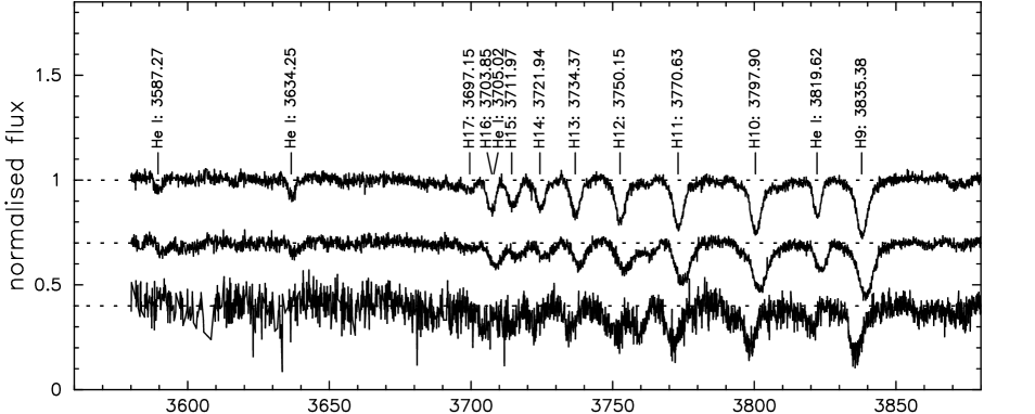
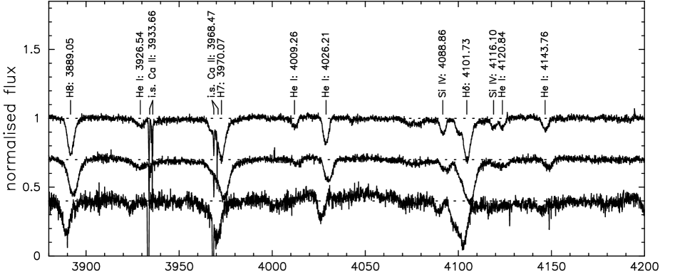
Figure 1: Normalised spectra in the wavelength range 3580–4500 Å of SMC~X$-$1 at orbital phase $\phi=0.06$ (top spectrum), LMC~X$-$4 at orbital phase $\phi=0.04$ (middle spectrum) and Cen~X$-$3 at orbital phase $\phi=0.09$ (bottom spectrum), respectively. The line identifications are shown above the spectrum of SMC~X$-$1. Note that the reddening of Cen~X$-$3 ($E(B-V)\sim 1.4$) clearly affects the S/N in this wavelength range.

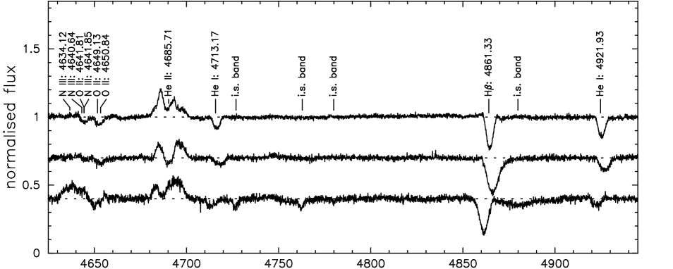
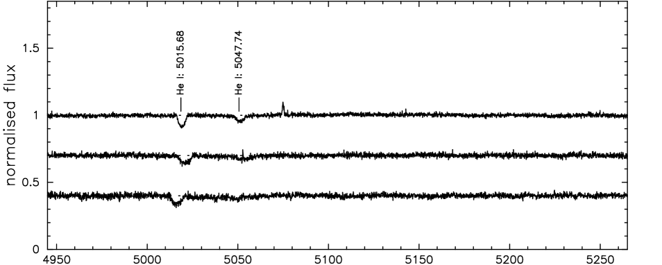
Figure 2: Normalised spectra in the wavelength range 4625–5585 Å of SMC~X$-$1 at orbital phase $\phi=0.06$ (top spectrum), LMC~X$-$4 at orbital phase $\phi=0.04$ (middle spectrum) and Cen~X$-$3 at orbital phase $\phi=0.09$ (bottom spectrum), respectively. The line identifications are shown above the spectrum of SMC~X$-$1.

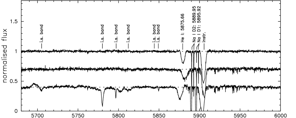
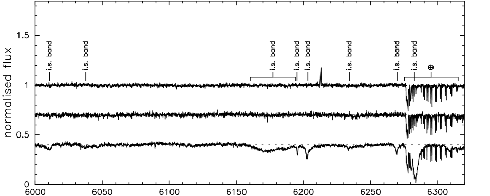
Figure 3: Normalised spectra in the wavelength range 5680–6640 Å of SMC~X$-$1 at orbital phase $\phi=0.06$ (top spectrum), LMC~X$-$4 at orbital phase $\phi=0.04$ (middle spectrum) and Cen~X$-$3 at orbital phase $\phi=0.09$ (bottom spectrum), respectively. The line identifications are shown above the spectrum of SMC~X$-$1.

2.3 Cen~X$-$3

Cen~X$-$3 was discovered by Chodil et al. (1967) and became the first detected binary X-ray pulsar (Giacconi et al. 1971; Schreier et al. 1972b). The $V=13.3$ mag optical counterpart V779~Cen was identified by Krzeminski (1974), an O6-7 II-III star (Ash et al. 1999) in a 2.09 d circular orbit with the 4.84 s X-ray pulsar. The optical light curve indicates the likely presence of an accretion disc, but no strong evidence is found for X-ray heating (Tjemkes et al. 1986). The X-ray light curve includes episodes of high and low X-ray flux with a characteristic timescale of 120–165 d (Priedhorsky & Terrell 1983; Paul et al. 2005).

Figure 4: Example of gaussian fits for the He i line at 4387.93 Å (upper panel), the He i line at 4713.17 Å (middle panel) and the He i line at 5047.74 Å (lower panel) in the spectrum of the B supergiant companion to SMC~X$-$1. The spectra and the gaussian fits are shown at four different quadratures. To better visualise the fits the spectra are smoothed. Note that the gaussian profile fits represent the rotationally broadened line profiles very well. Furthermore, the orbital motion of the B supergiant companion is easily observed.

Based on photographic spectra, Hutchings et al. (1979) derive $K_{\rm opt}=24\pm 6$ km s^-1, confirmed by Aslanov & Cherepashchuk (1982) who also report $K_{\rm opt}=24\pm 6$ km s^-1. The most recent radial-velocity measurements of V779~Cen are presented by Ash et al. (1999) who determine two very different values of $K_{\rm opt}$ based on two datasets obtained with the 4m Anglo-Australian Telescope and the RGO spectrograph. The wavelength range of these spectra is 4300–4700 Å; the spectral resolution $R\sim 3000$. Ash et al. (1999) discard the results of the first dataset and arrive at $K_{\rm opt}=24.4\pm 4.1$ km s^-1. The resulting neutron-star mass is M${}_{X}=1.21\pm 0.21$ M_☉ and the mass of the O-type companion M${}_{\rm opt}=20.5\pm 0.7$ M_☉.

Figure 5: Example of radial-velocity curves obtained from the H13 line at 3734.37 Å. Some datapoints are shown twice to better visualise trends with orbital phase. The error bars indicate 1 $\sigma$ errors. The lower panels show the residuals of the fit.

3 Observations

We have obtained high-resolution ($R\sim 40\,000$) spectra of the three systems with UVES (Dekker et al. 2000) on the VLT in service mode in the period October 2001 to March 2002 at Paranal, Chile. The total exposure time was 17.6 h spread over 13 exposures of 1400 s of SMC~X$-$1, 13 exposures of 2000 s of LMC~X$-$4 and 12 exposures of 1600 s of Cen~X$-$3. The instrument was used with standard setting “390+564” and a slit width of 1.0″. This yields a wavelength range of 3580–4500 Å in the blue arm and 4625–5585 Å and 5680–6640 Å in the red arm. To determine the orbital phase of the systems we used the ephemeris of Wojdowski et al. (1998), Levine et al. (2000) and Nagase et al. (1992) for SMC~X$-$1, LMC~X$-$4 and Cen~X$-$3, respectively (see Table 1). The log of observations is listed in Table 2.

In order to reduce the data to normalised spectra we used the UVES pipeline (version 1.2.0) and the ESO reduction package MIDAS (version 03SEPpl1.1). All raw echelle frames were bias and flatfield corrected. Subsequently the different orders were extracted using the optimal extraction routine available within the UVES pipeline. High signal-to-noise ($S/N\ga 50$) spectra extracted with this routine show a ripple effect. In our spectra this effect is only marginally present in some spectra of SMC~X$-$1 in the wavelength range 5100–5585 Å. This range contains the ${He\textsc{ii}}$ 5411.53 Å line, but we do not use it for the determination of the radial-velocity amplitude of the system (Sect. 4.2).

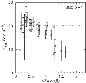
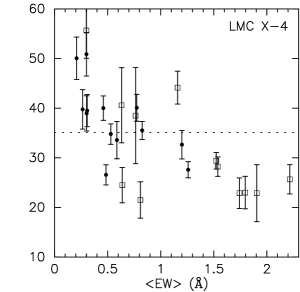
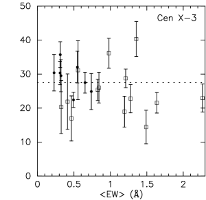
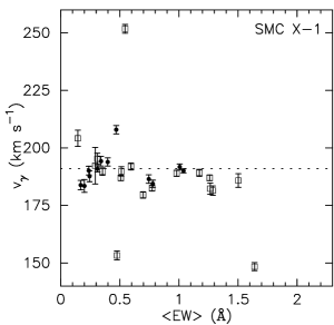
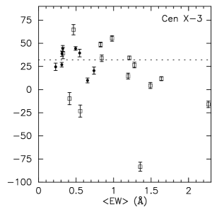
Figure 6: The upper panels show the radial-velocity amplitude ($K_{\rm opt}$ in km s^-1) measured for a given line as a function of its mean line equivalent width ($<{\rm EW}>$). The error bars indicate 1 $\sigma$ errors. Especially for SMC~X$-$1 a clear trend is visible with line strength: for large mean EW $K_{\rm opt}$ is systematically lower. The finally adopted $K_{\rm opt}$ is represented by the horizontal dotted line. The middle panels show the $\gamma$-velocity and the bottom panels show $K_{\rm opt}$ as a function of the line variability parameter $\eta$; lines with $\eta>9$ are rejected (see text for motivation). The lines that are rejected because of this and other criteria (such as blending) are represented by open squares. The filled circles indicate the lines that are used to determine the (mean) radial-velocity amplitude. These selections show less spread in $K_{\rm opt}$.

Cosmic ray hits were removed by rejecting the affected wavelength bins and subsequent interpolation. After this, the spectra were normalised by fitting the continuum with a spline over the whole wavelength range of one spectral arm. The normalised spectra of the three systems are shown in Figs. 1 to 3.

We verified the long-term stability of UVES by measuring the position of the interstellar lines of ${Ca\textsc{ii}}$ K at 3933.66 Å, ${Ca\textsc{ii}}$ H at 3968.47 Å, ${Na\textsc{i}}$ D1 at 5895.92 Å and ${Na\textsc{i}}$ D2 at 5889.95 Å for all spectra. This resulted in a deviation of less than 1 km s^-1 throughout the whole observing period of each system, i.e. several months.

Table 3: List of lines that have been fitted with a gaussian. The rest wavelength of the line is given as well as the mean equivalent width (EW, in Ångström) with its $1\sigma$ error. The magnitude of the variations in line EW is expressed as the ratio $\eta$ of the standard deviation of the line EW to the error on the mean EW. Rejected lines are indicated with a remark: lines marked with an “B” are blends; a “V” stands for lines exhibiting strong EW variations ($\eta>9$); a number (e.g. 0.5) indicates a deviation in the EW at that orbital phase. Electronic tables that contain the radial-velocity amplitude, EW and FWHM variations for each line are available as on-line material at the CDS.

		SMC~X$-$1			LMC~X$-$4			Cen~X$-$3
Identification	$\lambda_{\rm rest}$ (Å)	$\mu_{\rm EW}$ (Å)	$\eta$	Remarks	$\mu_{\rm EW}$ (Å)	$\eta$	Remarks	$\mu_{\rm EW}$ (Å)	$\eta$	Remarks
H Balmer series
H$\beta$	$4861.33$	$1.265(4)$	$44.1$	V,0.5	$1.905(7)$	$22.6$	V,0.5	$1.491(6)$	$20.4$	V,0.5
H$\gamma$	$4340.46$	$1.287(5)$	$24.2$	B,V,0.5	$1.796(8)$	$14.9$	B,V,0.5	$1.638(10)$	$8.6$	B,0.5
H$\delta$	$4101.73$	$1.503(7)$	$17.5$	B,V,0.5	$2.216(9)$	$7.6$	B,V,0.5	$2.264(16)$	$7.0$	B,0.5
H$\epsilon$	$3970.07$	$1.640(13)$	$8.5$	B,0.5	$1.742(11)$	$10.4$	B,V,0.5	$1.356(23)$	$22.7$	B,V,0.5
H8	$3889.05$	$1.173(4)$	$9.7$	V,0.5	$1.538(6)$	$10.0$	V,0.5	$1.278(11)$	$6.5$	0.5
H9	$3835.38$	$1.260(5)$	$9.2$	B?,V,0.5	$1.523(7)$	$9.2$	B?,V	$1.211(12)$	$7.9$	B?,0.5
H10	$3797.90$	$1.039(5)$	$8.2$		$1.259(7)$	$8.4$		$0.843(12)$	$5.9$	0.5
H11	$3770.63$	$1.007(6)$	$8.6$		$1.200(10)$	$6.8$		$0.980(18)$	$7.0$	0.5
H12	$3750.15$	$0.779(6)$	$6.6$		$0.638(10)$	$7.4$	B	$0.413(15)$	$5.3$	B
H13	$3734.37$	$0.745(6)$	$6.5$		$0.588(12)$	$6.1$		$0.548(22)$	$4.5$
H14	$3721.94$	$0.513(8)$	$5.9$	B	$-$	$-$		$-$	$-$
H15	$3711.97$	$0.470(11)$	$4.6$		$-$	$-$		$-$	$-$
H16	$3703.85$	$0.545(8)$	$8.3$	B	$0.764(237)$	$3.1$	B	$0.466(96)$	$3.0$	B
He I 3P-3D series
He i 2p-3d	$5875.66$	$0.981(5)$	$31.3$	V,0.0	$1.159(11)$	$8.6$	0.0	$1.194(7)$	$21.3$	V,0.0,0.5
He i 2p-4d	$4471.50$	$0.773(6)$	$12.3$	V,0.0	$0.775(8)$	$8.1$		$0.739(10)$	$6.7$
He i 2p-5d	$4026.21$	$0.697(4)$	$12.1$	V,0.0	$0.825(5)$	$8.7$		$0.653(8)$	$3.6$
He i 2p-6d	$3819.62$	$0.509(4)$	$11.3$	V,0.0	$0.460(5)$	$8.9$		$0.313(10)$	$2.9$
He i 2p-7d	$3705.02$	$0.476(9)$	$8.2$	B,0.0	$0.632(66)$	$4.4$	B	$0.556(152)$	$2.6$	B
He i 2p-8d	$3634.25$	$0.244(5)$	$5.7$		$0.208(7)$	$6.4$		$-$	$-$
He i 2p-9d	$3587.27$	$0.169(5)$	$7.2$		$-$	$-$		$-$	$-$
He I 1P-1D series
He i 2p-4d	$4921.93$	$0.595(3)$	$16.2$	V,0.0	$0.530(5)$	$7.0$		$0.323(5)$	$5.2$
He i 2p-5d	$4387.93$	$0.398(5)$	$6.5$		$0.302(6)$	$5.5$		$-$	$-$
He i 2p-6d	$4143.76$	$0.341(4)$	$6.1$		$0.301(6)$	$6.4$		$-$	$-$
He i 2p-7d	$4009.26$	$0.238(4)$	$4.8$		$-$	$-$		$-$	$-$
He I 3P-3S series
He i 2p-4s	$4713.17$	$0.311(4)$	$6.6$		$0.265(5)$	$4.6$		$0.228(6)$	$6.2$
He I 1S-1P series
He i 2s-3p	$5015.68$	$0.353(3)$	$10.9$	V,0.0	$0.307(5)$	$7.4$		$0.310(5)$	$4.2$
He I 1P-1S series
He i 2p-4s	$5047.74$	$0.201(4)$	$6.7$		$-$	$-$		$-$	$-$
Other lines
He ii 4-7	$5411.53$	$0.292(4)$	$42.5$	V,0.5	$0.809(7)$	$14.0$	V,0.5	$0.827(5)$	$11.0$	B,0.5
He ii 4-11	$4199.83$	$0.145(5)$	$9.7$	V,0.5	$0.485(7)$	$5.6$		$0.494(9)$	$4.2$
Si iv 4s-4p	$4088.86$	$0.310(4)$	$10.3$	V,0.0	$0.300(11)$	$6.6$	B	$0.326(12)$	$6.7$	B

4 Spectral Analysis

To obtain a radial-velocity measurement often the complete spectrum is cross-correlated with a template spectrum. This approach has many advantages when using spectra with relatively low spectral resolution and poor signal-to-noise. In our case the spectra are of such high quality that the radial-velocity amplitude can be determined for each line separately. The advantage of such a strategy is that it is possible to assess the influence of possible distortions due to e.g. X-ray heating and gravity darkening, as in these systems the OB star is irradiated by a powerful X-ray source ($L_{\rm opt}\simeq L_{X}$) and is filling its Roche-lobe. Furthermore, the extended OB-star wind is focused into a shadow wind which possibly produces a strong shock (a so-called photo-ionisation wake, see e.g. Blondin 1994; Kaper et al. 1994) where the fast shadow wind catches up with the stagnant flow inside the X-ray ionization zone. The shadow wind and photo-ionization wake induce orbital modulations of spectral lines formed in the stellar wind (i.e. strong spectral lines such as the first lines of the Balmer series and the strongest helium lines).

Figures 1 to 3 show that the spectra contain mostly lines that are identified with transitions from H and He i. Only a few He ii lines and some metal lines are detected, consistent with the modest metallicity of the Magellanic Clouds and OB supergiant spectral types. We show the spectra observed near X-ray eclipse (orbital phase $\phi\sim 0.0$). Some of the lines are blended or show a slight asymmetry. A comparison of the spectra obtained at different orbital phase reveals that several lines also vary in line strength. Still, Fig. 4 demonstrates that many lines are well represented by a gaussian profile (i.e. as one would expect for a rotationally broadened profile). Therefore, gaussian profiles are fit to all individual lines to determine the radial-velocity curve (Sect. 4.1). Subsequently, the observed line profiles are examined on asymmetry and variations with orbital phase (Sect. 4.2).

Figure 7: Equivalent width (EW) variations with orbital phase ($\phi$) observed in SMC~X$-$1. The error bars indicate 1 $\sigma$ errors and the dotted line the average value. Some datapoints are shown twice to better visualise trends with orbital phase. The value of the defined line variability parameter $\eta$ is indicated for each line. The upper panel shows the large variations in the He ii line at 5411.53 Å, the second panel shows the inverse behaviour of the He i line at 4471.50 Å, the third panel shows the variations of H$\epsilon$ at 3970.07 Å. A stable line is shown in the lower panel, i.e. the H12 line at 3750.15 Å. The EW ratio of the He ii and He i lines is sensitive to $T_{\rm eff}$ and can be used for spectral classification; apparently, the spectral type of SMC~X$-$1 varies with orbital phase. The variations are consistent with being caused by X-ray heating of the stellar surface facing the X-ray source.

4.1 Radial-velocity curves

We determine the line centre, and thus the Doppler shift with respect to the heliocentric restframe, by fitting the profile with a gaussian. The gaussian sets the full-width at half maximum (FWHM), the central line depth and the central wavelength of the profile, i.e. three free parameters. A $\chi^{2}$ minimalization procedure delivers the best fit gaussian profile and defines the accuracy of the fit parameters. Emission-line profiles, such as H$\alpha$, are not included in the fitting procedure.

The orbital parameters are accurately known from X-ray pulse time delay measurements (see Table 1). We assume the orbit to be circular, since in all cases the eccentricity $e\lesssim 0.008$. The remaining free parameters describing the radial-velocity curve are the radial-velocity amplitude, $K_{\rm opt}$, and the restframe velocity of the system, $v_{\gamma}$. In principle, a small shift in orbital phase could be present due to the inaccuracy of the orbital period, the period derivative, and mid-eclipse time (Table 1). The measured orbital phase shifts are not significantly different from zero, but are slightly larger than the phase shifts one may expect based on the accuracy of the ephemeres of these systems. The phase shift should be the same for all lines and has to be fixed to the average value during a second iteration.

A radial-velocity curve is obtained for each individual line; Fig. 5 displays for each system a radial-velocity curve representative for the spectral lines used to measure the radial-velocity amplitude. Note that the data points were obtained from several orbits of the system; the dozen spectra per system are evenly distributed with orbital phase, thanks to the service-mode observations allowing to obtain spectra spread over a period of more than one month.

Fig. 6 indicates that $K_{\rm opt}$ and $v_{\gamma}$ show quite some dispersion when comparing the radial-velocity curves of individual lines. $K_{\rm opt}$ shows a dependence on line strength and line variability, diagnostics that we will use to reject lines when determining the mean radial-velocity amplitude used to calculate the mass of the neutron star.

Figure 8: Full width at half maximum (FWHM) variations of the H$\gamma$ line at 4340.46 Å (upper panel) and the He i line at 4387.93 AA (lower panel) of SMC~X$-$1 as a function of orbital phase ($\phi$) in km s^-1. The error bars indicate 1 $\sigma$ errors and the dotted line the average value. Some datapoints are repeated once to better visualise trends with orbital phase. A maximum in FWHM is clearly seen around $\phi\sim 0.25$; a second, though much less pronounced maximum is visible at $\phi\sim 0.75$. Such FWHM variations are also detected in other lines, as well as in the systems LMC~X$-$4 and Cen~X$-$3.

4.2 Line Selection

As our observational strategy is aimed at the derivation of the radial-velocity curve based on individual lines, we select only lines that are well identified. Also, all lines that are (partially) blended, are rejected. In Table 3 this is indicated with a “B” as a remark.

In these high-mass X-ray binaries it is expected that at least some lines in the OB-star spectrum are affected by the presence of the X-ray pulsar companion (see e.g. Van Paradijs et al. 1978; Reynolds et al. 1993). In principle, one could model the photospheric line profiles of the OB supergiant companion by calculating a grid of many (thousands) surface elements, adopting for each surface element an intrinsic line profile, and obtaining the integrated line profile by a weighted integration of the (mainly by stellar rotation) Doppler-shifted intrinsic profiles of all visible surface elements. Such computationally demanding techniques have been successfully explored in stellar pulsation studies (e.g. Schrijvers et al. 1997) and in modeling photometric lightcurves of HMXBs (e.g. Heemskerk & Van Paradijs 1989). Also, variations in the intrinsic line profiles due to variations of surface temperature and gravity have been included (Schrijvers & Telting 1999), so that one could apply such a method to the case of an OB supergiant irradiated and deformed by a close and compact X-ray source. Although we have now made an advance in analysing spectra of the OB companions to X-ray pulsars by studying individual lines rather than cross-correlating complete spectra, we consider this modeling effort beyond the scope of the present paper, even though it has the potential to deliver very important information on the interpretation and analysis of the obtained spectra.

Table 4: Final selection of lines that is used for the determination of the radial-velocity amplitude ($K_{\rm opt}$) for each system. The three fit parameters are listed, i.e. the system velocity ($v_{\gamma}$), $K_{\rm opt}$, and a phase shift ($\Delta\phi$). The goodness of the fit is expressed as $\chi^{2}_{r}$. All errors are 1 $\sigma$.

	SMC~X$-$1				LMC~X$-$4				Cen~X$-$3
$\lambda_{\rm rest}$ (Å)	$v_{\gamma}$	$K_{\rm opt}$	$\Delta\phi$	$\chi^{2}_{r}$	$v_{\gamma}$	$K_{\rm opt}$	$\Delta\phi$	$\chi^{2}_{r}$	$v_{\gamma}$	$K_{\rm opt}$	$\Delta\phi$	$\chi^{2}_{r}$
$3797.90$	$190.0\pm 0.9$	$20.2\pm 1.2$	$0.01(1)$	$2.6$	$305.5\pm 1.1$	$27.6\pm 1.6$	$0.01(1)$	$1.6$	$-$	$-$	$-$	$-$
$3770.63$	$191.7\pm 1.3$	$18.1\pm 1.8$	$0.01(2)$	$3.8$	$321.5\pm 2.1$	$32.6\pm 2.9$	$-0.02(2)$	$3.2$	$-$	$-$	$-$	$-$
$3750.15$	$184.5\pm 1.6$	$18.4\pm 2.2$	$0.04(2)$	$4.3$	$-$	$-$	$-$	$-$	$-$	$-$	$-$	$-$
$3734.37$	$186.5\pm 1.8$	$18.1\pm 2.5$	$0.02(2)$	$4.9$	$306.2\pm 2.6$	$33.6\pm 3.8$	$0.02(2)$	$1.7$	$39.5\pm 4.1$	$32.1\pm 4.7$	$0.02(4)$	$0.9$
$3711.97$	$207.9\pm 1.8$	$20.4\pm 2.4$	$0.07(2)$	$0.9$	$-$	$-$	$-$	$-$	$-$	$-$	$-$	$-$
$4471.50$	$-$	$-$	$-$	$-$	$298.9\pm 1.9$	$40.1\pm 2.7$	$0.00(1)$	$2.7$	$20.5\pm 3.9$	$24.9\pm 5.3$	$0.08(4)$	$5.8$
$4026.21$	$-$	$-$	$-$	$-$	$290.2\pm 1.3$	$35.5\pm 1.8$	$0.00(1)$	$2.9$	$9.9\pm 2.6$	$27.5\pm 3.1$	$0.03(3)$	$3.3$
$3819.62$	$-$	$-$	$-$	$-$	$301.9\pm 1.7$	$40.0\pm 2.5$	$-0.01(1)$	$2.0$	$38.8\pm 2.8$	$35.7\pm 3.8$	$0.07(2)$	$0.7$
$3634.25$	$187.7\pm 2.4$	$20.5\pm 3.2$	$0.03(3)$	$2.0$	$312.1\pm 2.9$	$50.0\pm 4.3$	$-0.03(2)$	$0.8$	$-$	$-$	$-$	$-$
$3587.27$	$183.9\pm 2.1$	$19.0\pm 2.8$	$0.01(3)$	$1.0$	$-$	$-$	$-$	$-$	$-$	$-$	$-$	$-$
$4921.93$	$-$	$-$	$-$	$-$	$311.7\pm 1.5$	$34.8\pm 2.1$	$-0.02(1)$	$1.8$	$44.3\pm 3.3$	$29.5\pm 4.7$	$0.10(3)$	$3.0$
$4387.93$	$193.9\pm 1.8$	$23.7\pm 2.4$	$0.04(2)$	$3.1$	$328.6\pm 2.6$	$38.9\pm 3.6$	$-0.01(2)$	$1.4$	$-$	$-$	$-$	$-$
$4143.76$	$194.2\pm 2.1$	$25.6\pm 2.7$	$0.02(2)$	$3.7$	$315.3\pm 3.1$	$50.9\pm 4.4$	$-0.01(2)$	$1.6$	$-$	$-$	$-$	$-$
$4009.26$	$190.1\pm 1.9$	$20.4\pm 2.5$	$0.05(2)$	$1.8$	$-$	$-$	$-$	$-$	$-$	$-$	$-$	$-$
$4713.17$	$190.9\pm 1.3$	$22.3\pm 1.9$	$0.02(1)$	$2.3$	$315.7\pm 2.7$	$39.8\pm 4.0$	$0.00(2)$	$1.7$	$24.6\pm 4.0$	$30.4\pm 5.4$	$0.08(3)$	$1.6$
$5047.74$	$183.5\pm 2.8$	$21.7\pm 3.9$	$0.03(3)$	$3.0$	$-$	$-$	$-$	$-$	$-$	$-$	$-$	$-$
$5015.68$	$-$	$-$	$-$	$-$	$312.7\pm 2.4$	$39.5\pm 3.2$	$-0.03(2)$	$2.1$	$26.9\pm 2.5$	$30.3\pm 3.5$	$0.09(2)$	$1.7$
$4199.83$	$-$	$-$	$-$	$-$	$303.3\pm 1.3$	$26.6\pm 2.0$	$0.05(1)$	$0.6$	$44.4\pm 2.0$	$22.4\pm 2.3$	$0.03(2)$	$0.8$

A first step in this direction has been undertaken by Abubekerov et al. (2004); they model the line formation process taking X-ray heating and gravitational darkening into account. As the luminosity distribution and shape of the star are altered, the measured radial velocity, as well as the line equivalent width, depend on the depth of the line-forming region and orbital phase. Abubekerov et al. (2004) show that these effects will result in a reduction of the derived radial-velocity amplitude by several km s^-1.

That these effects manifest themselves in our observations is nicely demonstrated by the large EW variations of the He ii line at 5411.53 Å of SMC~X$-$1 (see Fig. 7). This line varies with about a factor $\sim 5$ in EW and reaches a maximum EW near $\phi\sim 0.5$. The He i line at 4471.50 Å (and also He i 5875.66 Å) shows the opposite behaviour and has a minimum strength at this orbital phase (see Fig. 7). Since a He i / He ii line ratio is sensitive to $T_{\rm eff}$ it can be used for spectral classification; however, traditionally the ratio of He i 4471 over He ii 4541, accessible in the blue spectrum, is used for spectral classification (Conti & Alschuler 1971; Lennon et al. 1993; Mokiem et al. 2005). Line ratios involving the He i 5876 and He ii 5412 lines have not (yet) been calibrated (Mokiem, priv. comm.). The observed variations in line ratio indicate a higher $T_{\rm eff}$ at the side of the OB star facing the X-ray source, and is evidence for X-ray heating in SMC~X$-$1. As a consequence, the spectral type of the optical companion to SMC~X$-$1 changes as function of binary aspect angle. A similar effect has been observed in the optical spectrum of V779~Cen, the O6 companion of Cen~X$-$3 (Hutchings et al. 1979).

The derived value of the radial-velocity amplitude shows a dependence on line strength (Fig. 6). Furthermore, the observed variations in EW also increase with line strength. As illustrated above, these variations likely reflect distortions of the line forming region due to e.g. X-ray heating and the (disturbed) stellar wind. Since $K_{\rm opt}$ should be a unique value, we investigate whether a selection criterion can be defined to reject lines that are affected by these distortions and thus do not yield a sound measurement of $K_{\rm opt}$.

Table 5: Weighted mean values of the radial velocity for each spectrum, indicated by its orbital phase ($\phi$) for SMC~X$-$1, LMC~X$-$4, and Cen~X$-$3. All errors are 1 $\sigma$.

SMC~X$-$1		LMC~X$-$4		Cen~X$-$3
$\phi$	$<v_{\rm rad}>$	$\phi$	$<v_{\rm rad}>$	$\phi$	$<v_{\rm rad}>$
	(km s-1)		(km s-1)		(km s-1)
$0.062$	$8.42\pm 1.06$	$0.037$	$6.45\pm 1.50$	$0.095$	$14.96\pm 2.97$
$0.096$	$19.04\pm 1.02$	$0.138$	$29.28\pm 2.23$	$0.234$	$22.87\pm 2.10$
$0.186$	$16.58\pm 0.77$	$0.247$	$40.06\pm 1.38$	$0.284$	$31.47\pm 1.98$
$0.255$	$24.42\pm 1.17$	$0.274$	$30.03\pm 1.60$	$0.337$	$14.12\pm 2.59$
$0.315$	$14.70\pm 0.95$	$0.337$	$24.84\pm 1.24$	$0.354$	$18.43\pm 2.75$
$0.458$	$4.98\pm 0.84$	$0.388$	$25.04\pm 1.33$	$0.462$	$-10.75\pm 2.86$
$0.537$	$-9.37\pm 1.01$	$0.418$	$23.23\pm 1.10$	$0.512$	$-21.61\pm 2.42$
$0.645$	$-18.46\pm 1.24$	$0.533$	$-14.69\pm 1.54$	$0.681$	$-26.12\pm 2.19$
$0.707$	$-19.07\pm 1.08$	$0.694$	$-30.90\pm 1.21$	$0.746$	$-18.81\pm 1.76$
$0.765$	$-16.47\pm 0.89$	$0.743$	$-34.06\pm 1.17$	$0.761$	$-23.29\pm 2.07$
$0.837$	$-19.83\pm 0.87$	$0.809$	$-30.86\pm 1.16$	$0.831$	$-24.32\pm 2.34$
$0.909$	$-8.22\pm 0.77$	$0.927$	$-17.96\pm 1.19$	$0.515$	$-14.55\pm 1.98$
$0.961$	$-1.85\pm 1.09$	$0.927$	$-17.95\pm 1.12$

To measure these distortions we apply a velocity moment analysis, with which one can determine the equivalent width (EW), central velocity, standard deviation ($\sigma$) and skewness ($\tau$) of a given line. The n^th moment ($\mu_{n}$) of a distribution $f(v)$ in velocity $v$ is given by:

$$\mu_{n}=\frac{\int{v^{n}\leavevmode\nobreak\ f(v)\leavevmode\nobreak\ dv}}{\int{f(v)\leavevmode\nobreak\ dv}},$$ (1)

and

$$\mu_{0}=\int{f(v)\leavevmode\nobreak\ dv}.$$ (2)

For such a distribution the EW is proportional to $\mu_{0}$ and the central velocity to $\mu_{1}$. The standard deviation ($\sigma$) and skewness ($\tau$) are often defined as:

$$\sigma^{2}=\frac{\int{(v-\mu_{1})^{2}\leavevmode\nobreak\ f(v)\leavevmode\nobreak\ dv}}{\mu_{0}},$$ (3)

and

$$\tau=\frac{\int{(v-\mu_{1})^{3}\leavevmode\nobreak\ f(v)\leavevmode\nobreak\ dv}}{\mu_{0}\leavevmode\nobreak\ \sigma^{3}},$$ (4)

in which the skewness ($\tau$) is a measure of the asymmetry of the distribution. For a gaussian profile the skewness $\tau$ is zero; if $\tau\neq 0$ the spectral line is not well represented by a gaussian. If so, one can not use a gaussian to fit the line in order to measure its radial velocity, as we did in Sect. 4.1. It turns out that for the lines that are not blended, $\tau$ is consistent with being equal to zero within the error. Note, however, that the error on $\tau$ is too large to measure any significant deviations from zero, because it depends on the error on $\mu$ and $\sigma$ to the third power (see Eq. 4). The EW and central velocity (first moment) are much more accurately determined and are consistent with the respective values derived from the gaussian profile fits.

For each line we determine whether the line EW varies significantly by comparing the deviation in EW to the error on the mean EW (Table 3). Note that these values are not equal; the error on the mean depends on the error in EW of the individual spectra, while the standard deviation is the spread in the distribution of EWs. Since the strongest lines are formed in the outer layers of the stellar photosphere and/or in the extended stellar wind these lines are expected to be most affected by X-ray heating, gravity darkening, etc., and will thus show intrinsic variations when the system revolves. The observed trend in $K_{\rm opt}$ with $v_{\gamma}$ (Fig. 6) also indicates that the stronger lines are formed further out in the stellar atmosphere and wind (an effect called Balmer progression, see e.g. Crampton et al. 1985; Abubekerov et al. 2004). We define a line variability parameter $\eta$ to formulate a selection criterion (Table 3). This parameter is defined as the ratio of the standard deviation of the EW variations to the error on the mean EW. The main motivation behind this definition is that the EW is in principle not sensitive to radial-velocity variations, i.e. the key parameter that we want to measure in the spectra. However, $\eta$ turns out to be an accurate probe of intrinsic line profile variability. Other methods to measure line profile variability (e.g. the temporal variance spectrum analysis method introduced by Fullerton et al. 1996) are sensitive to radial-velocity variations.

We select $\eta=9$ as the value above which lines are rejected. These lines are indicated with a “V” in Table 3. The threshold value for $\eta$ is chosen arbitrarily, but is a reproducable and objective means to quantify line profile variations. As it is an averaged quantity, the $\eta$ threshold does not reject lines exhibiting only modest EW variations and having relatively large errors on the measured EWs (e.g. the H$\epsilon$ at 3970.07 Å shown in Fig. 7). On the other hand, it does reject some lines that have highly accurately determined EWs and that exhibit hardly any EW variations with orbital phase. To test the impact of the chosen value for the $\eta$ threshold on the obtained value of the radial-velocity amplitude, we have evaluated the results for different values of $\eta$. Including all lines for which $\eta<8$ then $K_{\rm opt}$ is $20.8\pm 1.5$, $35.7\pm 1.8$, and $27.5\pm 2.3$ km s^-1 for SMC~X$-$1, LMC~X$-$4, and Cen~X$-$3, respectively. Similarly, we obtain $20.0\pm 1.2$, $34.2\pm 1.3$, and $26.2\pm 2.7$, respectively, if we select the lines with $\eta<13$. As expected, we obtain a lower value of $K_{\rm opt}$ for a higher value of $\eta$, and vice versa, while the error on the result increases when including lines that show more intrinsic variations. Still, the values for $K_{\rm opt}$ agree within the error for the applied range in $\eta$.

We now fix the threshold to $\eta=9$; to ensure that the lines with $\eta<9$ and small variations concentrated around $\phi\sim 0.0$ or $\phi\sim 0.5$, are rejected, we mark these in Table 3 listing the orbital phase at which these variations are concentrated. Note that most of these lines are already marked with a “V”, i.e. rejected based on the $\eta$ threshold.

The full width at half maximum (FWHM) of the line also varies as a function of orbital phase $\phi$. This behaviour is especially visible in the Balmer series lines of hydrogen, most prominent in the stronger lines. Figure 8 shows that the FWHM increases when the system revolves from X-ray eclipse to $\phi\sim 0.25$, where it reaches a maximum before declining again. At $\phi\sim 0.75$ another, though smaller increase in FWHM is detected. The helium (and some other metallic) lines also show FWHM variations, but less pronounced and not as periodic as observed in the hydrogen lines. Furthermore, these FWHM variations are best seen in SMC~X$-$1 and LMC~X$-$4, but are less clear in Cen~X$-$3.

Apparently, if one would use these lines to determine the (projected) stellar rotation velocity, one would arrive at a larger value of $v\sin{i}$ when the system is looked upon from a side view. This may be due to the elongated shape of the star as it is filling its Roche lobe, as evidenced by the observed ellipsoidal variations. The dependence on line strength would be explained by the fact that the line forming region is further out in the atmosphere when the line is stronger. This would, however, not explain the difference in amplitude of this effect observed between $\phi\sim 0.25$ and $\phi\sim 0.75$.

Differences in spectral appearance when comparing spectra obtained at $\phi\sim 0.25$ and $\phi\sim 0.75$ are well known to occur in spectroscopic binaries. The “Struve-Sahade” effect (Struve 1937; Sahade 1962) is the apparent strengthening of the secondary spectrum of a hot binary when the secondary is approaching and the corresponding weakening of the lines when it is receding (see Gies et al. 1997 for an observational overview). The cause of this effect may be the presence of a gas stream (bow shock, wind collision) trailing the secondary in its orbit (Sahade 1959; Gies et al. 1997). Hydrodynamical simulations of SMC~X$-$1 by Blondin (1994) indicate that a collision of wind material from the shadow wind with material in the X-ray ionisation zone is present in the system. Perhaps that this shocked material introduces the difference in amplitude observed in the FWHM of the strong Balmer lines that are formed in the stellar wind.

As we do not have a clear explanation for these variations in FWHM, we investigate the possible influence of this effect on the determination of $K_{\rm opt}$. Note that the stronger Balmer lines are already excluded from the radial-velocity analysis on the basis of the EW variations. We fix the FWHM on its mean value, its maximum and its minimum and refit the lines. It turns out that the measurement of the centre of the line profile is not affected much by these FWHM variations. The derived radial-velocity amplitude, $K_{\rm opt}$, is the same within its errors in all cases. Therefore, we decide not to exclude more lines based on a FWHM variation criterion (most of the lines showing this effect were excluded on other grounds anyway).

4.3 Radial-velocity amplitude

Table 4 shows the final selection of lines for which good fits to the radial-velocity curve are obtained, resulting in a measurement of $K_{\rm opt}$ and $v_{\gamma}$. Since the phase shift should be equal for all lines in one system, we refit all lines with the phase shift fixed to the weighted average, i.e. $\triangle\phi$ is 0.026, -0.003, and 0.065 for SMC~X$-$1, LMC~X$-$4, and Cen~X$-$3, respectively. Fixing these values does not influence the other parameters much; they are the same within their errors.

Figure 9: Radial-velocity curves obtained from weighing the radial velocities of all selected lines per observation. Some datapoints are shown twice to better visualise trends with orbital phase. The error bars indicate 1 $\sigma$ errors multiplied by $\chi_{r}$ to obtain a $\chi^{2}_{r}=1$. Note that $v_{\gamma}$ has been set to zero.

To avoid sytematic errors while determining the final mean value of $K_{\rm opt}$ we shift all determined line centres to equal $v_{\gamma}$. The weighted mean values of $v_{\gamma}$ are $191\pm 6$ km s^-1, $306\pm 10$ km s^-1 and $32\pm 13$ km s^-1 for SMC~X$-$1, LMC~X$-$4 and Cen~X$-$3, respectively. Then we calculate the weighted mean of the radial velocity for each spectrum (see Table 5). The average dataset we fit in the same way as the individual lines, which results in the three radial-velocity curves shown in Fig. 9. The goodness of the fits with respect to the number of degrees of freedom (d.o.f.) are $\chi^{2}_{r}/{\rm d.o.f}=9.8/12$, $\chi^{2}_{r}/{\rm d.o.f}=9.1/12$ and $\chi^{2}_{r}/{\rm d.o.f}=7.2/11$ for SMC~X$-$1, LMC~X$-$4 and Cen~X$-$3, respectively. The error bars indicate 1 $\sigma$ errors multiplied by $\chi_{r}$ to obtain a $\chi^{2}_{r}=1$. The residuals to the fit do not show any further evidence for systematic effects with orbital phase, as is the case for e.g. Vela~X$-$1 (Van Kerkwijk et al. 1995b; Barziv et al. 2001). The final values of $K_{\rm opt}$ are $20.2\pm 1.1$ km s^-1, $35.1\pm 1.5$ km s^-1 and $27.5\pm 2.3$ km s^-1 for SMC~X$-$1, LMC~X$-$4 and Cen~X$-$3, respectively. The accuracy of the determination of $K_{\rm opt}$ has been significantly improved (by a factor 2–4) compared to previous measurements (and comparable to and consistent with Val Baker et al. (2005) in the case of SMC~X$-$1). These values are subsequently used to calculate the mass of the optical companion and the X-ray source.

Figure 10: Selection of lines for which we measured the rotational broadening. Each diagram includes a solid line representing the model that we applied; the dotted line represents the continuum. To better visualise the model, the spectra are smoothed with 7 resolution elements. The top panels show the modelled spectral lines of SMC~X$-$1, the second and third row include lines of LMC~X$-$4 and the two bottom rows show lines of Cen~X$-$3.

5 The neutron star masses

In order to measure the mass of the neutron star and its optical companion we apply the mass function. For an orbit with eccentricity $e$ it can be shown that this is defined as:

$$M_{\rm opt}=\frac{K_{\rm X}^{3}P\left(1-e^{2}\right)^{\frac{3}{2}}}{2\pi G\sin^{3}i}\left(1+q\right)^{2}$$ (5)

and

$$M_{\rm X}=\frac{K_{\rm opt}^{3}P\left(1-e^{2}\right)^{\frac{3}{2}}}{2\pi G\sin^{3}i}\left(1+\frac{1}{q}\right)^{2},$$ (6)

where $M_{\rm opt}$ and $M_{\rm X}$ are the masses of the optical component and the X-ray source, respectively, $K_{\rm opt}$ and $K_{\rm X}$ are the semi-amplitude of the radial-velocity curve, $P$ is the period of the orbit and $i$ is the inclination of the orbital plane to the line of sight. The mass ratio $q$ is defined as:

$$q=\frac{M_{\rm X}}{M_{\rm opt}}=\frac{K_{\rm opt}}{K_{\rm X}}$$ (7)

The values for $K_{\rm X}$ and $P$ can be obtained very accurately from X-ray pulse timing delay measurements (Wojdowski et al. 1998; Levine et al. 2000; Nagase et al. 1992). The VLT/UVES spectra provide a value for $K_{\rm opt}$. For the determination of the inclination of the system we follow the approach of Rappaport & Joss (1983), who showed that:

$$\sin i\approx\frac{\sqrt{1-\beta^{2}\left(\frac{R_{\rm L}}{a}\right)^{2}}}{\cos\theta_{e}}$$ (8)

where $R_{\rm L}$ is the Roche-lobe radius of the optical component, $\beta$ is the ratio of the radius of the optical component to $R_{\rm L}$ (i.e. a Roche-lobe filling factor), $a$ is the separation of the centres of mass of the two components, and $\theta_{\rm e}$ is the semi-eclipse angle of the compact object (see also Joss & Rappaport (1984) for a review on mass determinations in X-ray binaries).

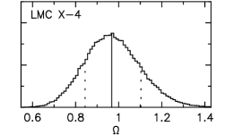
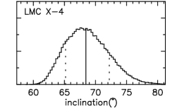
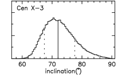
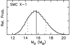
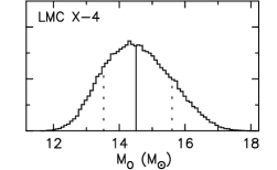
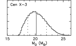
Figure 11: Resulting probability distributions from the Monte-Carlo simulations for SMC~X$-$1 (left column), LMC~X$-$4 (middle column) and Cen~X$-$3 (rigth column). Shown are the ratio of the rotational and orbital frequency ($\Omega$), the inclination angle ($i$), the ratio of the Roche-lobe radius and the orbital separation ($R_{\rm L}/a$) and the masses of both components ($M_{\rm opt}$ & $M_{\rm X}$) of the three systems. The mean value and $1\sigma$ limits are shown with solid and dotted lines, respectively.

The ratio of the Roche-lobe radius and the orbital separation can be approximated by:

$$\frac{R_{L}}{a}\approx A+B\log q+C\log^{2}q\,.$$ (9)

The values of the constants $A$, $B$ and $C$ were determined by Rappaport & Joss (1983) to be:

$$A\approx 0.398-0.026\Omega^{2}+0.004\Omega^{3}$$ (10)

$$B\approx-0.264+0.052\Omega^{2}-0.015\Omega^{3}$$ (11)

$$C\approx-0.023-0.005\Omega^{2},$$ (12)

where $\Omega$ is the ratio of the rotational frequency of the optical companion to the orbital frequency of the system; in case of synchronous rotation $\Omega=1$. However, the timescale at which these systems are expected to synchronise is slightly longer than the timescale at which the orbit will circularise (for a detailed description see e.g. Hut 1981). Therefore, these systems may still be in the process of synchronising the optical companion to the orbit, whereas their orbits have already become circular. The fact that the orbital periods of all three systems are decreasing, suggests that the donor stars are rotating slower than synchronous and that tidal forces are transferring orbital angular momentum to synchronise the system.

It is possible to determine $\Omega$ by measuring the projected rotation velocity $v_{\rm rot}\sin{i}$ of the OB companion using the spectra at $\phi=0.0$. We use the grid of unified stellar atmosphere/wind models of early-type supergiants computed by Lenorzer et al. (2004) using cmfgen (Hillier & Miller 1998). First we select the lines that correspond to lines included in the model. Subsequently, we select the model atmosphere that reproduces the observed line spectrum best. The normalised flux of the model is then scaled to yield exactly the observed EW. The models that correspond best to our selection of lines are named “AR1Ia”, “AR1III” and “O9III-AR2III” for SMC~X$-$1, LMC~X$-$4 and Cen~X$-$3, respectively by Lenorzer et al. (2004). Note that the names of these models correspond to a set of model parameters describing the model and not to the observational spectral type naming convention. These models are subsequently convolved with a rotational broadening profile with a limb-darkening coefficient 0.6, as described by Gray (1992), to determine the value of $v_{\rm rot}\sin{i}$. This results in $170\pm 30$ km s^-1, $240\pm 25$ km s^-1 and $200\pm 40$ km s^-1 for SMC~X$-$1, LMC~X$-$4 and Cen~X$-$3, respectively. The selected lines and their corresponding best model are shown in Fig. 10. The rotational velocities required for a synchronous orbit are $185$ km s^-1, $250$ km s^-1 and $255$ km s^-1 for SMC~X$-$1, LMC~X$-$4 and Cen~X$-$3, respectively. We will find below that these correspond to rotation rates consistent with, though perhaps slightly slower than, a synchronous orbit.

Table 6: List of final values for the radial velocity amplitude ($K_{\rm opt}$) and the results from the output of the Monte-Carlo simulations, i.e. the values of the inclination angle ($i$), the ratio of the rotational and orbital frequency ($\Omega$), the ratio of the Roche-lobe radius and the orbital separation ($R_{\rm L}/a$), the radius of the optical companion ($R_{\rm opt}$), the orbital separation ($a$), and the masses of both components ($M_{\rm opt}$ & $M_{\rm X}$) of the three systems. All errors are 1 $\sigma$.

	SMC~X$-$1	LMC~X$-$4	Cen~X$-$3
$K_{\rm opt}$ (km s-1)	$20.2\pm 1.1$	$35.1\pm 1.5$	$27.5\pm 2.3$
$i$ ($\deg$)	$67^{+5}_{-4}$	$68^{+4}_{-3}$	$72^{+6}_{-5}$
$\Omega$	$0.91^{+0.21}_{-0.19}$	$0.97^{+0.14}_{-0.12}$	$0.75\pm 0.13$
$R_{\rm L}/a$	$0.61^{+0.02}_{-0.03}$	$0.59^{+0.01}_{-0.02}$	$0.63^{+0.01}_{-0.02}$
$R_{\rm opt}$ (R☉)	$16.4^{+1.0}_{-1.1}$	$7.8^{+0.3}_{-0.4}$	$12.1\pm 0.5$
$a$ (R☉)	$26.6\pm 0.8$	$13.3\pm 0.3$	$19.1^{+0.6}_{-0.5}$
$M_{\rm opt}$ (M☉)	$15.7^{+1.5}_{-1.4}$	$14.5^{+1.1}_{-1.0}$	$20.2^{+1.8}_{-1.5}$
$M_{\rm X}$ (M☉)	$1.06^{+0.11}_{-0.10}$	$1.25^{+0.11}_{-0.10}$	$1.34^{+0.16}_{-0.14}$

Since for Roche-lobe overflow systems $\beta\gtrsim 0.9$ (Avni & Bahcall 1975), we follow the approach of Rappaport & Joss (1983) and adopt that $\beta$ is in the range $0.9-1.0$. Thus, given a set of $K_{\rm opt}$, $P$, $a_{\rm X}\sin{i}$ and $\theta_{\rm e}$, we can determine by means of Monte-Carlo simulations a 1$\sigma$ confidence range for the values of $R_{\rm L}/a$, $i$, $M_{\rm opt}$ and $M_{\rm X}$ (see Rappaport & Joss 1983; Van Kerkwijk et al. 1995a).

Since in these systems soft X-rays are absorbed by the extended stellar wind of the optical companion, the eclipse lasts longer at low energies (up to $\sim 5$ keV), depending on the density structure of the stellar wind of the optical companion (e.g. for 4U~1700$-$37 the eclipse at energies up to $\sim 2$ keV lasts almost twice as long as at $\sim 6$ keV; see Haberl et al. 1994; Van der Meer et al. 2005). Therefore, we prefer $\theta_{\rm e}$ determinations obtained from X-ray observations at high energies (see Table 1). For Cen~X$-$3 these measurements are available. An accurate modelling of the X-ray light curve of multiple observations obtained with SAS-3/XTCA in the energy range $7.9-20$ keV by Clark et al. (1988) results in a value of $\theta_{\rm e}=32.9\degr\pm 1.4\degr$. They do not list an error on their value, so we use the standard deviation in their $\theta_{\rm e}$ distribution. For SMC~X$-$1 and LMC~X$-$4 no detailed modelling has been performed and $\theta_{\rm e}$ measurements are mainly reported for older X-ray missions. We use the range $26\degr-30.5\degr$ for SMC~X$-$1 based on observations of Primini et al. (1976) ($28.2\degr\pm 0.9\degr$, $2-6$ keV, SAS-3), Bonnet-Bidaud & Van der Klis (1981) ($29.9\degr\pm 0.2\degr$, $2-12$ keV, COS-B) and Schreier et al. (1972a) ($29.1\degr\pm 2.8\degr$, $2-6$ keV, Uhuru). For LMC~X$-$4 we adopt the range $25\degr-29\degr$ based on observations of Li et al. (1978) ($29.0\degr\pm 2.5\degr$, $6-12$ keV, SAS-3), White (1978) ($26.2\degr\pm 1.1\degr$, $2-16$ keV, ARIEL V) and Pietsch et al. (1985) ($27.1\degr\pm 1.0\degr$, $2-7$ keV, EXOSAT).

Using the defined input distributions for the Monte-Carlo simulations, we can determine the distributions for $i$, $\Omega$, $R_{\rm L}/a$, $R_{\rm opt}$, $a$, $M_{\rm opt}$ and $M_{\rm X}$. All the results are listed in Table 6 and some of the corresponding distributions are shown in Fig 11. The masses of the neutron stars become: $M_{\rm X}=1.06^{+0.11}_{-0.10}$ M_☉ for SMC~X$-$1, $M_{\rm X}=1.25^{+0.11}_{-0.10}$ M_☉ for LMC~X$-$4 and $M_{\rm X}=1.34^{+0.16}_{-0.14}$ M_☉ for Cen~X$-$3 at a $1\sigma$ confidence level. Compared to the mass determinations listed in Sect. 2 the error on the neutron star mass is reduced by at least a factor two.

The masses and radii of the OB companion stars all lie in the range of 15–20 M_☉ and 8–16 R_☉, respectively, in line with previous values (Van Kerkwijk et al. 1995a). Conti (1978) and Kaper (2001) show that for these stars a higher mass is expected based on their spectral classification and conclude that these stars are undermassive for their luminosity. This may be due to the phase of mass transfer prior to the supernova forming the neutron star in the system. A detailed modelling of the optical spectra of the OB companions will be presented in a forthcoming paper.

Figure 12: Neutron Star (NS) masses in X-ray binaries, NS$-$NS binaries and NS$-$White Dwarf (WD) binaries obtained from Stairs (2004) and references therein. The indicated masses of SMC~X$-$1, LMC~X$-$4 and Cen~X$-$3 are obtained from this study. The error bars correspond to 1 $\sigma$ errors. This plot clearly suggests that neutron stars do not all have the same “canonical” mass. Note that although 4U~1700$-$37 most probably is a neutron star, it could be a black hole.

6 The neutron star mass distribution

Abubekerov et al. (2004) present a new method to derive the radial velocity curves for HMXB systems in which the optical component is deformed due to the (partial) filling of its Roche-lobe. They show that these systems are affected by gravitational darkening and by X-ray heating of the surface of the optical component. This can result in an underestimate of the radial velocity amplitude of the optical component and therefore in an underestimate of the mass of the neutron star. Since this will mostly affect systems hosting a bright X-ray source, Roche-lobe overflow systems will suffer most from this effect, i.e. the systems discussed in this paper. With our VLT/UVES observations it is possible for the first time to accurately determine the radial velocity amplitude of each absorption line separately. We showed that for lines that vary in EW the radial velocity is indeed underestimated by several km s^-1, consistent with the predictions of Abubekerov et al. (2004). By applying our carefully chosen selection criteria, we anticipate for these effects.

We conclude that with our observations we have significantly improved the accuracy of the determination of the radial-velocity amplitude, and subsequently the determination of the neutron star mass in these three systems. Whereas some HMXB systems have shown to host a neutron star with a mass significantly higher than 1.4 M_☉, as is the case for Vela X$-$1 and possibly 4U 1700$-$37, the mass of SMC~X$-$1 is low, $1.06^{+0.11}_{-0.10}$ M_☉. The masses of LMC~X$-$4 and Cen~X$-$3 are $1.25^{+0.11}_{-0.10}$ and $1.34^{+0.16}_{-0.14}$ M_☉, respectively. The mass of SMC~X$-$1 is just above the minimum neutron star mass of $\sim 1$ M_☉ and significantly different from the mass of the neutron star in Vela X$-$1. We conclude that the neutron stars in HMXBs have different masses, i.e. they do not all have the same “canonical” mass. We illustrate our new mass derivations in Fig. 12, as part of the neutron star masses reported by Stairs (2004) and references therein for neutron stars in different types of systems.

7 Discussion

It remains to be explained why the mass of SMC~X$-$1 is well below 1.28 M_☉. The low mass may be the result of a different formation scenario, i.e. the electron-capture collapse of a degenerate ${O\textsc{}}$-${Ne\textsc{}}$-${Mg\textsc{}}$ core. Van den Heuvel (2004) argues that the generally low masses of neutron stars measured in binary radio pulsar systems may be due to a selection effect, as follows. Pfahl et al. (2002) noticed that there are two classes among the wide Be/X-ray binaries: (1) a substantial group with low orbital eccentricities, which indicates that their neutron stars received hardly any velocity kick in their formation events, and (2) a group with high orbital eccentricities, in which the neutron stars must have received a kick velocity of several hundreds of km s^-1 in their birth events.

It was subsequently noticed (Van den Heuvel 2004) that the low orbital eccentricities of 5 out of the 7 known double neutron stars in the galactic disc indicate that the second-born neutron stars in these systems received hardly any kick velocity during their birth events and thus appear to belong to the same low-kick class of neutron stars as the ones in the low-eccentricity Be/X-ray binaries. These second-born neutron stars in the low-eccentricity double neutron star systems all appear to have low masses, in the range $1.18-1.36$ M_☉. This fits excellently with neutron-star formation by the electron-capture collapse of a degenerate ${O\textsc{}}$-${Ne\textsc{}}$-${Mg\textsc{}}$ core, which is expected to form at the end of the evolution of stars that originated in the main-sequence mass-range 8 to about $13\pm 1$ M_☉ (Miyaji et al. 1980; Podsiadlowski et al. 2005; Kitaura et al. 2005). Stars with larger masses develop at the end of their lives a collapsing iron core, surrounded by convective shells with ${O\textsc{}}$- and ${Si\textsc{}}$-burning. The violent convection in these shells may create large density inhomogeneities in the layers surrounding the proto-neutron-star formed by the collapsing iron core. This may lead to large anisotropies in the neutrino transport through these layers, which may cause the neutron star to be imparted with a ”kick” velocity of some 500 km s^-1(Burrows & Hayes 1996; Scheck et al. 2004). Indeed, young single radio pulsars have large space velocities (Gunn & Ostriker 1970) and their velocity distribution is very well represented by a Maxwellian with a characteristic mean velocity of about 400 km s^-1 (Hobbs et al. 2005).

In the light of these findings the low mass of the neutron star in SMC~X$-$1 would be consistent with its formation by electron-capture collapse in a degenerate ${O\textsc{}}$-${Ne\textsc{}}$-${Mg\textsc{}}$ core. This would imply a main-sequence progenitor mass $\lesssim 14$ M_☉. Presently the companion of SMC~X$-$1 has a mass of about $16$ M_☉. Allowing for some mass loss by stellar wind, its mass just after the mass transfer and the formation of the neutron star would have been about $18$ M_☉.

With an explosive mass loss during the formation of the neutron star of about $1$ M_☉ and a few solar masses stellar wind mass loss from the neutron-star progenitor, the initial system must have had a mass $\gtrsim 22$ M_☉ (including the neutron-star mass). Thus, a progenitor system of $13$ M_☉+$9$ M_☉ (or $14$ M_☉ + $8$ M_☉) would be consistent with the present system configuration. A potential problem with such a configuration is that conservation of mass and orbital angular momentum during mass transfer would lead to a fairly wide presupernova system, such that the present orbital period of $\sim 3.9$ days would be hard to understand, unless a large amount of orbital angular momentum has been lost with relatively little mass (at most a few solar masses) from the system. We thus conclude that the low mass of the neutron star in SMC~X$-$1 is consistent with formation by electron-capture collapse, provided that a relatively large amount of orbital angular momentum was lost from the system during the first phase of mass transfer.