Outer boundary conditions for Einstein’s field equations in harmonic coordinates

Abstract

We analyze Einstein’s vacuum field equations in generalized harmonic coordinates on a compact spatial domain with boundaries. We specify a class of boundary conditions which is constraint-preserving and sufficiently general to include recent proposals for reducing the amount of spurious reflections of gravitational radiation. In particular, our class comprises the boundary conditions recently proposed by Kreiss and Winicour, a geometric modification thereof, the freezing-$\Psi_{0}$ boundary condition and the hierarchy of absorbing boundary conditions introduced by Buchman and Sarbach. Using the recent technique developed by Kreiss and Winicour based on an appropriate reduction to a pseudo-differential first order system, we prove well posedness of the resulting initial-boundary value problem in the frozen coefficient approximation. In view of the theory of pseudo-differential operators it is expected that the full nonlinear problem is also well posed. Furthermore, we implement some of our boundary conditions numerically and study their effectiveness in a test problem consisting of a perturbed Schwarzschild black hole.

I Introduction

A common way to deal with the numerical simulation of wave propagation on an infinite domain is to replace the latter by a finite computational domain $\Sigma$ with artificial boundary $\partial\Sigma$. Boundary conditions at $\partial\Sigma$ must then be specified such that the resulting Cauchy problem is well posed. Additionally, the artificial boundary must be as transparent as possible to the physical problem on the infinite domain in the sense that it does not introduce too much spurious reflection from the boundary surface. The construction of such absorbing boundary conditions has received significant attention for wave problems in acoustics, electromagnetism, meteorology, and solid geophysics (see [1] for a review).

In this article, we construct absorbing boundary conditions for Einstein’s field equations in generalized harmonic coordinates. In these coordinates, one obtains a system of ten coupled quasi-linear wave equations for the ten components of the metric field. Therefore, ten boundary conditions must be imposed. However, it is important to realize that not all ten components of the metric represent physical degrees of freedom, so that one cannot simply apply the known results from the scalar wave equation directly to the ten wave equations for the metric components. Instead, one has to take into account the fact that the metric is subject to the harmonic condition which yields four constraints. In the absence of boundaries, it is possible to show that it is sufficient to solve these constraints along with their time derivatives on an initial Cauchy surface; the Bianchi identities and the evolution equations then guarantee that the constraints are satisfied everywhere and at each time. When timelike boundaries are present, four constraint-preserving boundary conditions need to be specified at $\partial\Sigma$ in order to insure that no constraint-violating modes propagate into the computational domain. This reduces the ten degrees of freedom to six. Another four degrees of freedom are related to the residual gauge freedom in choosing harmonic coordinates and fixing the geometry of the boundary surface. Therefore, one is left with two degrees of freedom which are related to the gravitational radiation. The challenge, then, is to specify boundary conditions at $\partial\Sigma$ which preserve the constraints, form a well posed initial-boundary value problem (IBVP) and minimize spurious reflections of gravitational radiation from the boundary. Additionally, one might want to require that gauge and constraint-violating modes propagate out of the domain without too much reflection.

Constraint-preserving boundary conditions for the harmonic system have been proposed before in [2, 3, 4, 5] and tested numerically in [3, 6, 7, 8, 9, 10]. The boundary conditions of [2, 3] are a combination of homogeneous Dirichlet and Neumann conditions, for which well posedness can be shown by standard techniques. On the other hand, the conditions of [2, 3] are likely to yield large spurious reflections of gravitational radiation and probably do not give a good approximation to the solution on the unbounded domain. Inhomogeneous boundary conditions which allow for a matching to a characteristic code are also considered in [3], but in this case the well posedness of the problem is not established. The boundary conditions of [5] are of the Sommerfeld type, and the well posedness of the resulting IBVP has been shown, at least in the frozen coefficient approximation. Finally, the boundary conditions presented in [4] contain second derivatives of the metric fields and freeze the Weyl scalar $\Psi_{0}$ to its initial value. As discussed below, this condition serves as a good first approximation to an absorbing condition. In this paper, we generalize the first order boundary conditions of [5] to the full nonlinear case, and also obtain more general second order boundary conditions that are very similar to the conditions presented in [4]. Furthermore, we obtain a class of constraint-preserving higher order boundary conditions which are flexible enough to incorporate the recently proposed hierarchy of absorbing outer boundary conditions proposed in [11, 12].

There has been a considerable amount of work on constructing well posed constraint-preserving boundary conditions for Einstein’s field equations. A well posed IBVP for Einstein’s vacuum equations was presented in Ref. [13]. This work, which is based on a tetrad formulation, recasts the evolution equations into first order symmetric hyperbolic quasilinear form with maximally dissipative boundary conditions [14, 15], for which (local in time) well posedness is guaranteed [16]. There has been a substantial effort to obtain well posed formulations for the more commonly used metric formulations of gravity using similar mathematical techniques (see [3, 17, 18, 19] for partial results). A different technique for showing the well posedness of the IBVP is based on the frozen coefficient principle where one freezes the coefficients of the evolution and boundary operators. In this way, the problem is simplified to a linear, constant coefficient problem on the half-space which can be solved explicitly by using a Fourier-Laplace transformation [20]. This method yields a simple algebraic condition (the determinant condition) which is necessary for the well posedness of the IBVP. Sufficient conditions for the well posedness of the frozen coefficient problem were developed by Kreiss [21]. Kreiss’ theorem provides a stronger form of the determinant condition whose satisfaction leads to well posedness if the evolution system is strictly hyperbolic. One of the key results in [21] is the construction of a smooth symmetrizer for the problem for which well posedness can be shown via an energy estimate in the frequency domain. Using the theory of pseudo-differential operators, it is expected that the verification of Kreiss’ condition also leads to well posedness for quasilinear problems, such as Einstein’s field equations. Work based on the verification of the Kreiss condition in the Einstein case is given in [22, 9]. In particular, generalized harmonic gauge and second order boundary conditions similar to the ones considered here were analyzed in [9]. However, since in those cases the evolution system is not strictly hyperbolic, it is not clear if those results are sufficient for well posedness. Kreiss’ theorem was generalized to symmetric hyperbolic systems in [23] but their treatment assumed maximally dissipative boundary conditions. On the other hand, the recent work by Kreiss and Winicour [5] introduces a new pseudo-differential first order reduction of the wave equation which leads to a strictly hyperbolic system. Using this reduction they are able to verify Kreiss’ condition and in this way show well posedness of the IBVP for Einstein’s field equations in harmonic coordinates.

We use this frozen coefficient technique in order to analyze the well posedness of the IBVPs resulting from our different boundary conditions. To this end, we consider small amplitude, high frequency perturbations of a given smooth background solution. In this case, the problem reduces to a system of ten decoupled wave equations on a frozen metric background on the half space with linear boundary conditions. By performing a suitable coordinate transformation which leaves the half space domain invariant, one can obtain all the metric coefficients to be those of the flat metric with the exception of the component of the shift normal to the boundary (see also [9]). We then prove using the Fourier-Laplace technique and Kreiss’ theorem that our frozen coefficient problem is well posed. In view of the existence of a smooth symmetrizer and the theory of pseudo-differential operators [24], it is expected that one can show well posedness of the full nonlinear problem as well.

This paper is organized as follows. In Sec. II we summarize the generalized harmonic formulation of general relativity. In Sec. III we study the resulting wave evolution equations for the ten components of the metric on a manifold of the form $M=[0,T]\times\Sigma$, where $\Sigma$ is a three-dimensional compact manifold with smooth boundary $\partial\Sigma$, and we present several possibilities for first, second and higher order boundary conditions, where here the order refers to the highest derivative of the metric appearing in the condition. In the first order case, in Sec. III.1, we use the harmonic constraint to impose four Dirichlet boundary conditions for the constraint propagation system. Next, we specify two boundary conditions in terms of the shear of the outgoing null congruence associated with the two-dimensional cross sections of the boundary surface. These conditions are a geometric modification of the boundary conditions presented by Kreiss and Winicour [5]. Finally, we specify four more boundary conditions with some absorbing properties on the gauge modes corresponding to the residual gauge freedom. In Sec. III.2 we present second order boundary conditions. One of the advantages of allowing for second derivatives of the metric is that one can formulate boundary conditions for the Weyl curvature scalar $\Psi_{0}$, which has some attractive properties. First, $\Psi_{0}$ (with respect to a suitably chosen tetrad) represents the incoming radiation at past null infinity. Second, the Weyl tensor from which $\Psi_{0}$ is constructed is a gauge-invariant quantity in the weak field limit of gravity. Third, if spacetime is a small perturbation of a Schwarzschild black hole, as is the case near the boundary if the boundary is far enough from the strong field region, $\Psi_{0}$ (with respect to a tetrad adapted to the Schwarzschild background) is invariant with respect to infinitesimal coordinate transformations and tetrad rotations. A boundary condition considered in the literature is the so-called freezing-$\Psi_{0}$ condition [13, 25, 26, 27, 4, 9, 19, 10], which freezes $\Psi_{0}$ to its initial value. An estimate for the amount of spurious reflections of gravitational radiation was given in [11]. There, a new hierarchy ${\cal B}_{L}$, $L=1,2,3,...$, of conditions on $\Psi_{0}$ was also derived with the property of being perfectly absorbing for linearized gravitational waves with angular momentum number smaller than or equal to $L$. Generalizations of these conditions which take into account correction terms from the curvature were presented in [12]. In order to incorporate these conditions into our analysis, we consider boundary conditions of arbitrarily high order in Sec. III.3. In Sec. IV we use the method by Kreiss and Winicour to show the well posedness of the resulting IBVPs in the frozen coefficient approximation. In particular, we allow for a non-trivial shift vector, which is important in view of the generalization to the quasi-linear case. In this sense, our results generalize the work in Ref. [5] to non-trivial shifts and boundary conditions of arbitrarily high order. Next, in Sec. V, we obtain estimates for the amount of spurious reflections for the boundary conditions constructed in this article and perform numerical tests based on a perturbed Schwarzschild black hole. Finally, we conclude in Sec. VI.

II The field equations in generalized harmonic coordinates

In this section we review the formulation of Einstein’s field equations in generalized harmonic coordinates [28, 29]

$$H^{c}=\Box_{g}x^{c}=g^{ab}\Gamma^{c}{}_{ab}\;,$$ (1)

where $H^{c}$ are given functions on $M$, $g_{ab}$ is the spacetime metric and $\Box_{g}=-g^{ab}\nabla_{a}\nabla_{b}$ and $\Gamma^{c}{}_{ab}$ denote the corresponding d’Alembertian operator and Christoffel symbols, respectively. Instead of adopting the gauge condition (1), we find it convenient to choose a fixed background manifold $(M,\mbox{\em\r{g}\hskip 0.85358pt}_{ab})$ and replace (1) by ${\cal C}^{c}=0$, where the vector field ${\cal C}^{c}$ is given by

$${\cal C}^{c}=g^{ab}\left(\Gamma^{c}{}_{ab}-\Gamma{}^{\mbox{\r{~}}}{}^{c}{}_{ab}\right)-H^{c}.$$ (2)

Here, $H^{c}$ is a given vector field on $M$ and $\Gamma{}^{\mbox{\r{~}}}{}^{c}{}_{ab}$ are the Christoffel symbols corresponding to the background metric $\mbox{\em\r{g}\hskip 0.85358pt}_{ab}$. In the particular case where the background manifold is Minkowski spacetime and standard Cartesian coordinates are chosen on $M$, $\Gamma{}^{\mbox{\r{~}}}{}^{c}{}_{ab}$ vanishes, and the condition ${\cal C}^{c}=0$ reduces to Eq. (1). The advantage of using ${\cal C}^{c}$ is that, unlike $\Box_{g}x^{c}$, it transforms as a vector field since the difference between the two Christoffel symbols,

$$C^{c}{}_{ab}\equiv\Gamma^{c}{}_{ab}-\Gamma{}^{\mbox{\r{~}}}{}^{c}{}_{ab}=\frac{1}{2}g^{cd}\left(\nabla{}^{\mbox{\r{~}}}{}_{a}h_{bd}+\nabla{}^{\mbox{\r{~}}}{}_{b}h_{ad}-\nabla{}^{\mbox{\r{~}}}{}_{d}h_{ab}\right),$$ (3)

forms a tensor field. Here and in the following, $h_{ab}=g_{ab}-\mbox{\em\r{g}\hskip 0.85358pt}_{ab}$ denotes the difference between the dynamical metric $g_{ab}$ and the background metric $\mbox{\em\r{g}\hskip 0.85358pt}_{ab}$. Since $\nabla{}^{\mbox{\r{~}}}{}_{c}\mbox{\em\r{g}\hskip 0.85358pt}_{ab}=0$, one could also replace $\nabla{}^{\mbox{\r{~}}}{}_{c}h_{ab}$ with $\nabla{}^{\mbox{\r{~}}}{}_{c}g_{ab}$ in Eq. (3); however, we prefer to express our equations in terms of the difference field $h_{ab}$ instead of the metric $g_{ab}$. A condition that is related to ${\cal C}^{c}=0$ was used in [30] for imposing spatial harmonic coordinates.

The curvature tensor corresponding to the metric $g_{ab}$ can be written as

$$R^{a}{}_{bcd}=\mbox{\em\r{R}}^{a}{}_{bcd}+2\nabla{}^{\mbox{\r{~}}}{}_{[c}C^{a}{}_{d]b}+2C^{a}{}_{e[c}C^{e}{}_{d]b}\;,$$ (4)

where $\mbox{\em\r{R}}^{a}{}_{bcd}$ denotes the curvature tensor with respect to the background metric $\mbox{\em\r{g}\hskip 0.85358pt}_{ab}$. Inserting Eq. (3) into (4) and using $\nabla{}^{\mbox{\r{~}}}{}_{a}g^{cd}=-C^{c}{}_{ab}g^{bd}-C^{d}{}_{ab}g^{bc}$, one obtains,

$$R_{abcd} = \frac{1}{2}\left(\nabla{}^{\mbox{\r{~}}}{}_{c}\nabla{}^{\mbox{\r{~}}}{}_{b}h_{ad}-\nabla{}^{\mbox{\r{~}}}{}_{d}\nabla{}^{\mbox{\r{~}}}{}_{b}h_{ac}+\nabla{}^{\mbox{\r{~}}}{}_{d}\nabla{}^{\mbox{\r{~}}}{}_{a}h_{cb}-\nabla{}^{\mbox{\r{~}}}{}_{c}\nabla{}^{\mbox{\r{~}}}{}_{a}h_{bd}\right)$$ (5)

$$+ g_{ef}C^{e}{}_{bc}C^{f}{}_{ad}-g_{ef}C^{e}{}_{bd}C^{f}{}_{ac}+\frac{1}{2}\left(g_{ae}\mbox{\em\r{R}}^{e}{}_{bcd}-g_{be}\mbox{\em\r{R}}^{e}{}_{acd}\right).$$

From this, we obtain the corresponding expression for the Ricci tensor,

$$R_{ab} = \frac{1}{2}g^{cd}\left(-\nabla{}^{\mbox{\r{~}}}{}_{c}\nabla{}^{\mbox{\r{~}}}{}_{d}h_{ab}-\nabla{}^{\mbox{\r{~}}}{}_{a}\nabla{}^{\mbox{\r{~}}}{}_{b}h_{cd}+\nabla{}^{\mbox{\r{~}}}{}_{a}\nabla{}^{\mbox{\r{~}}}{}_{c}h_{bd}+\nabla{}^{\mbox{\r{~}}}{}_{b}\nabla{}^{\mbox{\r{~}}}{}_{c}h_{ad}\right)$$ (6)

$$+ g_{ef}g^{cd}\left(C^{e}{}_{ac}C^{f}{}_{bd}-C^{e}{}_{ab}C^{f}{}_{cd}\right)-g^{cd}\mbox{\em\r{R}}^{e}{}_{cd(a}g_{b)e}\;.$$

On the other hand, we have

$$\nabla_{a}{\cal C}_{b} = g^{cd}\left(\nabla{}^{\mbox{\r{~}}}{}_{a}\nabla{}^{\mbox{\r{~}}}{}_{c}h_{bd}-\frac{1}{2}\,\nabla{}^{\mbox{\r{~}}}{}_{a}\nabla{}^{\mbox{\r{~}}}{}_{b}h_{cd}\right)-2\,C^{c}{}_{da}\,g_{be}\,C^{e}{}_{cf}\,g^{df}$$ (7)

$$- g_{ef}\,g^{cd}\,C^{e}{}_{ab}\,C^{f}{}_{cd}-\nabla_{a}H_{b}\;.$$

Subtracting the symmetric part of Eq. (7) from Eq. (6) we obtain

$${\cal E}_{ab} = g^{cd}\nabla{}^{\mbox{\r{~}}}{}_{c}\nabla{}^{\mbox{\r{~}}}{}_{d}h_{ab}-2\,g_{ef}g^{cd}C^{e}{}_{ac}C^{f}{}_{bd}-4\,C^{c}{}_{d(a}g_{b)e}C^{e}{}_{cf}g^{df}$$ (8)

$$+ 2\,g^{cd}\mbox{\em\r{R}}^{e}{}_{cd(a}g_{b)e}-2\,\nabla_{(a}H_{b)}\,,$$

where ${\cal E}_{ab}\equiv-2R_{ab}+2\nabla_{(a}{\cal C}_{b)}$. Using the twice contracted Bianchi identities we also obtain,

$$\nabla^{b}\left({\cal E}_{ab}-\frac{1}{2}g_{ab}g^{cd}{\cal E}_{cd}\right)=\nabla^{b}\nabla_{b}{\cal C}_{a}+R_{a}{}^{b}{\cal C}_{b}\;.$$ (9)

The Cauchy problem for Einstein’s vacuum equations in generalized harmonic coordinates on an infinite domain of the form $M=[0,T]\times\mathbb{R}^{3}$ can be formulated in the following two steps. First, specify initial data on the hypersurface $\Sigma_{0}:=\{0\}\times\mathbb{R}^{3}$. For this, let $n^{a}$ and $\mbox{\em\r{n}\hskip 0.85358pt}^{a}$ denote the future-pointing unit normals to $\Sigma_{0}$ with respect to the metrics $g_{ab}$ and $\mbox{\em\r{g}\hskip 0.85358pt}_{ab}$, respectively. Notice that the corresponding one-forms, $n_{a}$ and $\mbox{\em\r{n}\hskip 0.85358pt}_{a}$, are proportional to each other: $n_{a}=\alpha\,\mbox{\em\r{n}\hskip 0.85358pt}_{a}$. Decompose the dynamical metric in the form

$$g_{ab}=-\alpha^{2}\mbox{\em\r{n}\hskip 0.85358pt}_{a}\mbox{\em\r{n}\hskip 0.85358pt}_{b}+\gamma_{cd}\left(\delta^{c}{}_{a}-\beta^{c}\mbox{\em\r{n}\hskip 0.85358pt}_{a}\right)\left(\delta^{d}{}_{b}-\beta^{d}\mbox{\em\r{n}\hskip 0.85358pt}_{b}\right),$$

where $\gamma_{cd}\mbox{\em\r{n}\hskip 0.85358pt}^{c}=0$, $\beta^{c}\mbox{\em\r{n}\hskip 0.85358pt}_{c}=0$. The pull-back of $\gamma_{ab}$ on $\Sigma_{0}$ is the metric $\bar{g}_{ab}$ induced by $g_{ab}$ on $\Sigma_{0}$, and $\alpha$ and $\beta^{a}$ are generalized lapse and shift. Next, solve the Hamiltonian and momentum constraints $n^{a}(2R_{ab}-g_{ab}g^{cd}R_{cd})=0$ for the induced metric $\bar{g}_{ab}$ and the extrinsic curvature, $k_{ab}$. Then, solve the equation ${\cal C}^{a}=0$ which yields [31, 4]

$$\dot{\alpha} = \beta^{a}\mbox{\em\r{D}\hskip 0.85358pt}_{a}\alpha-\alpha^{2}\gamma^{ab}k_{ab}-\alpha(\mbox{\em\r{n}\hskip 0.85358pt}_{a}H^{a}+\gamma_{ab}\beta^{a}H^{b}),$$ (10)

$$\dot{\beta}^{a} = \beta^{b}\mbox{\em\r{D}\hskip 0.85358pt}_{b}\beta^{a}-\alpha\gamma^{ab}\mbox{\em\r{D}\hskip 0.85358pt}_{b}\alpha+\alpha^{2}\gamma^{ab}\gamma^{cd}\left[\mbox{\em\r{D}\hskip 0.85358pt}_{c}\gamma_{bd}-\frac{1}{2}\mbox{\em\r{D}\hskip 0.85358pt}_{b}\gamma_{cd}-\gamma_{bc}\gamma_{de}H^{e}\right],$$ (11)

where a dot refers to the Lie derivative with respect to $\mbox{\em\r{n}\hskip 0.85358pt}^{a}$, and D̊  denotes the connection on $\Sigma_{0}$ which is induced by $\nabla{}^{\mbox{\r{~}}}{}$. Here, we have assumed that $\nabla{}^{\mbox{\r{~}}}{}_{a}\mbox{\em\r{n}\hskip 0.85358pt}_{b}=0$ for simplicity. Equations (10,11) can be solved by either first choosing $\alpha$, $\beta^{a}$ and $H^{a}$ which fixes $\dot{\alpha}$ and $\dot{\beta}^{a}$ or by choosing $\alpha$, $\beta$, $\dot{\alpha}$ and $\dot{\beta}^{a}$ and solving for the vector field $H^{a}$. The quantities $\alpha$, $\dot{\alpha}$, $\beta^{a}$, $\dot{\beta}^{a}$, $\gamma_{ab}$ and $k_{ab}$ determine the initial data for $h_{ab}$ and $\dot{h}_{ab}\equiv\pounds_{\mbox{\em\r{n}\hskip 0.85358pt}}h_{ab}$ by taking into account that

$$\dot{\gamma}_{ab}=\left(-2\alpha k_{cd}+\pounds_{\beta}\gamma_{cd}\right)(\delta^{c}{}_{a}+\mbox{\em\r{n}\hskip 0.85358pt}^{c}\mbox{\em\r{n}\hskip 0.85358pt}_{a})(\delta^{d}{}_{b}+\mbox{\em\r{n}\hskip 0.85358pt}^{d}\mbox{\em\r{n}\hskip 0.85358pt}_{b}).$$

The second step consists in finding a solution $h_{ab}$ on $M$ of the nonlinear wave equation (8) with ${\cal E}_{ab}=0$ subject to the initial data specified on $\Sigma_{0}$. The results in [33, 32] show that there exists a unique solution to this problem, at least if $T$ is small enough. Finally, we observe that the evolution equations (8) with ${\cal E}_{ab}=0$ imply that [4]

$$n^{a}\nabla_{a}{\cal C}^{b}=n_{a}(2R^{ab}-g^{ab}g_{cd}R^{cd})+(\gamma^{ac}n^{b}-n^{a}\gamma^{bc})\nabla_{c}{\cal C}_{a}\;.$$ (12)

Since on $\Sigma_{0}$ the Hamiltonian and momentum constraints and ${\cal C}^{a}=0$ are satisfied, it follows that $\dot{\cal C}^{a}=0$. The evolution system for the harmonic constraint variables, Eq. (9) with ${\cal E}_{ab}=0$, then guarantees that ${\cal C}_{a}=0$ everywhere on $M$ since it has the form of a linear homogeneous wave equation for ${\cal C}_{a}$ with trivial initial data ${\cal C}_{a}=0$, $\dot{\cal C}_{a}=0$. In the next section, we analyze the Cauchy problem when the infinite domain $\mathbb{R}^{3}$ is replaced by a bounded domain $\Sigma$.

III Outer boundary conditions

We wish to study the evolution equations (8) with ${\cal E}_{ab}=0$ on a manifold of the form $M=[0,T]\times\Sigma$, where $\Sigma$ is a three-dimensional compact manifold with smooth boundary $\partial\Sigma$. We assume that the boundary surface ${\cal T}=[0,T]\times\partial\Sigma$ is timelike and that the three-dimensional surfaces $\Sigma_{t}=\{t\}\times\Sigma$ are spacelike. The cross section $S_{t}=\{t\}\times\partial\Sigma$ constitutes the boundary of $\Sigma_{t}$. For the following, let $n^{a}$ denote the future-pointing unit normal to the time-slices $\Sigma_{t}$ and $s^{a}$ the unit outward normal to the two surface $S_{t}$ as embedded in $\Sigma_{t}$. These vector fields are defined with respect to the dynamical metric $g_{ab}$ and not the background metric $\mbox{\em\r{g}\hskip 0.85358pt}_{ab}$. Therefore,

$$g_{ab}n^{a}n^{b}=-1\,,\qquad g_{ab}n^{a}s^{b}=0\,,\qquad g_{ab}s^{a}s^{b}=1\,.$$

The vector fields $n^{a}$ and $s^{a}$ allow us to construct a Newman-Penrose null tetrad $\{l^{a},k^{a},m^{a},\bar{m}^{a}\}$

$$l^{a} = \frac{1}{\sqrt{2}}\left(n^{a}+s^{a}\right),\qquad k^{a}=\frac{1}{\sqrt{2}}\left(n^{a}-s^{a}\right),\qquad$$ (13)

$$m^{a} = \frac{1}{\sqrt{2}}\left(v^{a}+i\,w^{a}\right),\qquad\bar{m}^{a}=\frac{1}{\sqrt{2}}\left(v^{a}-i\,w^{a}\right),$$ (14)

where $v^{a}$ and $w^{a}$ are two mutually orthogonal unit vector fields which are normal to $n^{a}$ and $s^{a}$ (with respect to the metric $g_{ab}$). Notice that this null tetrad is naturally adapted to the two-surfaces $S_{t}$; it is unique up to rescaling of the real null vectors $l^{a}$ and $k^{a}$ and up to a rotation $m^{a}\mapsto e^{i\varphi}m^{a}$, $\bar{m}^{a}\mapsto e^{-i\varphi}\bar{m}^{a}$ of the complex null vectors $m^{a}$ and $\bar{m}^{a}$ about an angle $\varphi$.

Since the evolution equations have the form of ten wave equations (see Eq. (8)), we need to specify ten boundary conditions on ${\cal T}$. These ten boundary conditions can be divided into constraint-preserving boundary conditions, boundary conditions controlling the physical radiation, and boundary conditions that control the gauge freedom. Constraint-preserving boundary conditions make sure that solutions with constraint-satisfying initial data satisfy the constraints for each $0<t<T$. Since there are four constraints, namely ${\cal C}^{c}=0$, and these constraints obey a set of wave equations on their own (see Eq. (9)), there are four constraint-preserving boundary conditions. Gravitational radiation has two degrees of freedom, so we need to provide two boundary conditions responsible for controlling the physical radiation. The remaining four boundary conditions control the gauge freedom.

In the following, we discuss several possibilities for fixing such boundary conditions. We divide them into first, second and higher order boundary conditions, where here the order refers to the highest number of derivatives of $h_{ab}$ appearing in the boundary conditions. These families of boundary conditions are discussed next. In Sec. IV, the well posedness of the resulting IBVPs in the frozen coefficient approximation is proven.

III.1 First order boundary conditions

In the first order case, constraint-preserving boundary conditions are specified through

$${\cal C}_{c}\equiv g^{ab}\left(\nabla{}^{\mbox{\r{~}}}{}_{a}h_{bc}-\frac{1}{2}\nabla{}^{\mbox{\r{~}}}{}_{c}h_{ab}\right)-H_{c}\;\hat{=}\;0,$$ (15)

where here and in the following, the notation $\;\hat{=}\;$ means an equality which holds on ${\cal T}$ only. These four boundary conditions are Dirichlet conditions for the constraint propagation system, Eq. (9) with ${\cal E}_{ab}=0$. Since this system is a linear homogeneous wave equation for ${\cal C}_{a}$ on the curved background $(M,g_{ab})$, these boundary conditions imply (by uniqueness) that solutions of this system with trivial initial data ${\cal C}_{a}=0$, $\dot{\cal C}_{a}=0$ are identically zero. Using $g^{ab}=-2\,l^{(a}k^{b)}+2\,m^{(a}\bar{m}^{b)}$, the four conditions (15) are equivalent to

$$0 \;\hat{=}\; {\cal C}_{c}l^{c}\;\hat{=}\;-D_{lm\bar{m}}-D_{kll}+D_{m\bar{m}l}+D_{\bar{m}ml}-H_{l}\;,$$ (16)

$$0 \;\hat{=}\; {\cal C}_{c}k^{c}\;\hat{=}\;-D_{lkk}-D_{km\bar{m}}+D_{m\bar{m}k}+D_{\bar{m}mk}-H_{k}\;,$$ (17)

$$0 \;\hat{=}\; {\cal C}_{c}m^{c}\;\hat{=}\;-D_{lkm}-D_{klm}+D_{mlk}+D_{\bar{m}mm}-H_{m}\;,$$ (18)

where we have defined the tensor field $D_{cab}\equiv\nabla{}^{\mbox{\r{~}}}{}_{c}h_{ab}$ and where the indices $l$, $k$, $m$, $\bar{m}$ refer to contraction with $l^{a}$, $k^{a}$, $m^{a}$ and $\bar{m}^{a}$, respectively. Notice that equation (18) comprises two real-valued equations.

Next, we consider the shear associated with the null congruence along the outgoing null vector field $l^{a}$. This quantity is defined as

$$\sigma^{(l)}_{ab}=\left(\gamma_{a}{}^{c}\gamma_{b}{}^{d}-\frac{1}{2}\,\gamma_{ab}\gamma^{cd}\right)\nabla_{c}l_{d}\;,$$ (19)

where $\gamma_{ab}=g_{ab}+n_{a}n_{b}-s_{a}s_{b}=2m_{(a}\bar{m}_{b)}$ is the induced metric on $S_{t}$. Notice that $\sigma^{(l)}_{ab}$ is normal to $n^{a}$ and $s^{a}$ and trace-free; hence it has two degrees of freedom. Furthermore, it depends on first derivatives of the metric. We impose the boundary condition

$$m^{a}m^{b}\sigma^{(l)}_{ab}\;\hat{=}\;q_{2}\;,$$ (20)

where $q_{2}$ is a given complex-valued function on ${\cal T}$. In order to express this condition in terms of $C^{c}{}_{ab}$ and background quantities, we first notice that the one-forms $n_{a}$ and $s_{a}$ are related to their corresponding background quantities $\mbox{\em\r{n}\hskip 0.85358pt}_{a}$ and $\mbox{\em\r{s}\hskip 0.85358pt}_{a}$ by

$$n_{a}=\alpha\,\mbox{\em\r{n}\hskip 0.85358pt}_{a}\;,\qquad s_{a}=\epsilon\,\mbox{\em\r{s}\hskip 0.85358pt}_{a}+\delta\,\mbox{\em\r{n}\hskip 0.85358pt}_{a}\;,$$

where $\alpha$, $\delta$ and $\epsilon$ are functions on ${\cal T}$ with $\alpha$ and $\epsilon$ being strictly positive. Next, we compute

$$\gamma_{a}{}^{c}\gamma_{b}{}^{d}\nabla_{c}l_{d}=\gamma_{a}{}^{c}\gamma_{b}{}^{d}\left(\nabla{}^{\mbox{\r{~}}}{}_{c}l_{d}-l_{e}C^{e}{}_{cd}\right).$$

Since $\{n_{a}\,,s_{a}\}$ and $\{\mbox{\em\r{n}\hskip 0.85358pt}_{a}\,,\mbox{\em\r{s}\hskip 0.85358pt}_{a}\}$ span the same vector space, $\gamma_{a}{}^{c}\gamma_{b}{}^{d}\nabla{}^{\mbox{\r{~}}}{}_{c}l_{d}=:{\cal K}{}^{\mbox{\r{~}}}{}^{(l)}_{ab}$ coincides with the second fundamental form of the two-surface $S_{t}$ as embedded in the background manifold $(M,\mbox{\em\r{g}\hskip 0.85358pt}_{ab})$ with respect to the normal vector field $\mbox{\em\r{g}\hskip 0.85358pt}^{ab}l_{b}$. Therefore,

$$\sigma^{(l)}_{ab}=\left(\gamma_{a}{}^{c}\gamma_{b}{}^{d}-\frac{1}{2}\,\gamma_{ab}\gamma^{cd}\right)\left({\cal K}{}^{\mbox{\r{~}}}{}^{(l)}_{cd}-l_{e}C^{e}{}_{cd}\right).$$

Since $\sqrt{2}\,l_{a}=(\alpha+\delta)\mbox{\em\r{n}\hskip 0.85358pt}_{a}+\epsilon\,\mbox{\em\r{s}\hskip 0.85358pt}_{a}$, ${\cal K}{}^{\mbox{\r{~}}}{}^{(l)}_{ab}$ is explicitly given by

$${\cal K}{}^{\mbox{\r{~}}}{}^{(l)}_{ab}=\frac{1}{\sqrt{2}}\gamma_{a}{}^{c}\gamma_{b}{}^{d}\left[(\alpha+\delta)\nabla{}^{\mbox{\r{~}}}{}_{c}\mbox{\em\r{n}\hskip 0.85358pt}_{d}+\epsilon\,\nabla{}^{\mbox{\r{~}}}{}_{c}\mbox{\em\r{s}\hskip 0.85358pt}_{d}\right].$$

For the following, it is important to notice that while ${\cal K}{}^{\mbox{\r{~}}}{}^{(l)}_{ab}$ depends on the metric fields $h_{ab}$, it does not depend on derivatives of $h_{ab}$. Finally, using Eq. (3), the boundary condition (20) can be expressed as

$$D_{lmm}-2D_{mlm}\;\hat{=}\;2\left(q_{2}-{\cal K}{}^{\mbox{\r{~}}}{}^{(l)}_{mm}\right).$$ (21)

Considering that $\sqrt{2}\,l^{a}\partial_{a}=n^{a}\partial_{a}+s^{a}\partial_{a}$, we see that the boundary conditions (16)-(18) and (21) yield generalized Sommerfeld conditions of the form $l^{a}\nabla{}^{\mbox{\r{~}}}{}_{a}u\;\hat{=}\;q$ for the metric components $u\in\{h_{m\bar{m}}\,,h_{kk}\,,h_{km}\,,h_{mm}\}$ where $q$ does not contain any derivatives along $l^{a}$. For this reason, we specify four more Sommerfeld-like conditions on the remaining metric components $h_{ll}$, $h_{lk}$, $h_{lm}$ and obtain the first order boundary conditions

$$D_{lll} \;\hat{=}\; p\;,$$ (22)

$$D_{llk} \;\hat{=}\; \pi\;,$$ (23)

$$D_{llm} \;\hat{=}\; q_{1}\;,$$ (24)

$$D_{lmm} \;\hat{=}\; 2D_{mlm}+2\left(q_{2}-{\cal K}{}^{\mbox{\r{~}}}{}^{(l)}_{mm}\right)\,,$$ (25)

$$D_{lm\bar{m}} \;\hat{=}\; -D_{kll}+D_{ml\bar{m}}+D_{\bar{m}lm}-H_{l}\;,$$ (26)

$$D_{lkm} \;\hat{=}\; -D_{klm}+D_{mlk}+D_{\bar{m}mm}-H_{m}\;,$$ (27)

$$D_{lkk} \;\hat{=}\; -D_{km\bar{m}}+D_{m\bar{m}k}+D_{\bar{m}mk}-H_{k}\;,$$ (28)

where $p$ and $\pi$ are real-valued given functions on ${\cal T}$ and $q_{1}$ and $q_{2}$ are complex-value given functions on ${\cal T}$, with $q_{2}=m^{a}m^{b}\sigma^{(l)}_{ab}$ representing the shear with respect to the outgoing null vector field $l^{a}$. With respect to a rotation $m\mapsto e^{i\varphi}m$ of the complex null vector, we have $q_{1}\mapsto e^{i\varphi}q_{1}$ and $q_{2}\mapsto e^{2i\varphi}q_{2}$; hence $q_{1}$ and $q_{2}$ have spin weights $1$ and $2$, respectively.

III.2 Second order boundary conditions

Next, we generalize the previous boundary conditions to second order boundary conditions, which depend on second derivatives of $h_{ab}$. The motivation for this is that such conditions can be used to reduce the amount of spurious reflections at the boundary surface. For example, the four boundary conditions (15) are Dirichlet conditions for the constraint propagation system, Eq. (9) with ${\cal E}_{ab}=0$, which means that constraint violations are reflected at the boundary [9]. Such reflections can be reduced by replacing the four Dirichlet conditions with Sommerfeld-like boundary conditions on the constraint variables ${\cal C}_{c}$, namely

$$l^{a}\nabla_{a}{\cal C}_{b}\;\hat{=}\;0\,.$$ (29)

These conditions were used in [4] and analyzed in [9]. As before, they imply that solutions to the constraint propagation system with trivial initial data vanish identically. But in contrast to the condition (15), the condition (29) allows most constraint violations generated inside the computational domain by numerical errors to leave the computational domain. In view of Eq. (7) these conditions yield

$$0\;\hat{=}\;l^{a}l^{b}\nabla_{a}{\cal C}_{b} \;\hat{=}\; -E_{llm\bar{m}}-E_{lkll}+E_{lm\bar{m}l}+E_{l\bar{m}ml}$$ (30)

$$- 2\,C^{cd}{}_{l}C_{lcd}-C^{c}{}_{ll}C_{cef}g^{ef}-l^{a}l^{b}\nabla_{a}H_{b}\;,$$

$$0\;\hat{=}\;l^{a}k^{b}\nabla_{a}{\cal C}_{b} \;\hat{=}\; -E_{llkk}-E_{lkm\bar{m}}+E_{lm\bar{m}k}+E_{l\bar{m}mk}$$ (31)

$$- 2\,C^{cd}{}_{l}C_{kcd}-C^{c}{}_{lk}C_{cef}g^{ef}-l^{a}k^{b}\nabla_{a}H_{b}\;,$$

$$0\;\hat{=}\;l^{a}m^{b}\nabla_{a}{\cal C}_{b} \;\hat{=}\; -E_{llkm}-E_{lklm}+E_{lmlk}+E_{l\bar{m}mm}$$ (32)

$$- 2\,C^{cd}{}_{l}C_{mcd}-C^{c}{}_{lm}C_{cef}g^{ef}-l^{a}m^{b}\nabla_{a}H_{b}\;,$$

where we have defined the tensor field $E_{cdab}\equiv\nabla{}^{\mbox{\r{~}}}{}_{c}\nabla{}^{\mbox{\r{~}}}{}_{d}h_{ab}$.

Next, we specify the complex Weyl scalar $\Psi_{0}$ at the boundary. Such boundary conditions have been proposed in the literature [13, 27, 26, 4, 9, 19, 25, 10]. In particular, freezing $\Psi_{0}$ to its initial value has been suggested as a good starting point for absorbing gravitational waves which propagate out of the computational domain. Recently, an analytic study [11] has shown that this freezing-$\Psi_{0}$ condition yields spurious reflections which decay as fast as $(kR)^{-4}$ for large $kR$, for monochromatic radiation with wavenumber $k$ and for an outer boundary with areal radius $R$. The Weyl scalar $\Psi_{0}$ is defined as

$$\Psi_{0}=R_{abcd}\,l^{a}\,m^{b}\,l^{c}\,m^{d}.$$

Using the expression (5) for the Riemann curvature tensor, we obtain

$$2\,\Psi_{0}=-E_{llmm}-E_{mmll}+2E_{(lm)lm}+2\,C^{c}{}_{lm}C_{clm}-2\,C^{c}{}_{ll}C_{cmm}+l_{a}\mbox{\em\r{R}}^{a}{}_{mlm}-m_{a}\mbox{\em\r{R}}^{a}{}_{llm}\;.$$

Therefore, the six boundary conditions specified so far have the form $l^{a}l^{b}\nabla_{a}\nabla_{b}u\;\hat{=}\;q$, where $u\in\{h_{m\bar{m}},h_{kk},h_{km},h_{mm}\}$, and $q$ depends on zeroth, first and second derivatives of $h_{ab}$ but only contains up to first-order derivatives with respect to $l^{a}$. We supplement these conditions with four similar conditions on the missing metric components $h_{ll}$, $h_{lk}$ and $h_{lm}$. The second order boundary conditions are then

$$E_{llll} \;\hat{=}\; p\;,$$ (33)

$$E_{lllk} \;\hat{=}\; \pi\;,$$ (34)

$$E_{lllm} \;\hat{=}\; q_{1}\;,$$ (35)

$$E_{llmm} \;\hat{=}\; -E_{mmll}+2\,E_{(lm)lm}+2\,C^{c}{}_{lm}C_{clm}$$ (36)

$$- 2C^{c}{}_{ll}C_{cmm}+l_{a}\mbox{\em\r{R}}^{a}{}_{mlm}-m_{a}\mbox{\em\r{R}}^{a}{}_{llm}-2\psi_{0}\;,$$

$$E_{llkm} \;\hat{=}\; -E_{lklm}+E_{lmlk}+E_{l\bar{m}mm}-2\,C^{cd}{}_{l}\,C_{mcd}$$ (37)

$$- C^{c}{}_{lm}C_{cef}g^{ef}-l^{a}m^{b}\nabla_{a}H_{b}\;,$$

$$E_{llm\bar{m}} \;\hat{=}\; -E_{lkll}+E_{lm\bar{m}l}+E_{l\bar{m}ml}-2\,C^{cd}{}_{l}\,C_{lcd}$$ (38)

$$- C^{c}{}_{ll}\,C_{cef}g^{ef}-l^{a}l^{b}\nabla_{a}H_{b}\;,$$

$$E_{llkk} \;\hat{=}\; -E_{lkm\bar{m}}+E_{lm\bar{m}k}+E_{l\bar{m}mk}-2\,C^{cd}{}_{l}\,C_{kcd}$$ (39)

$$- C^{c}{}_{lk}C_{cef}g^{ef}-l^{a}k^{b}\nabla_{a}H_{b}\;,$$

where $p$ and $\pi$ are real-valued given functions on ${\cal T}$, and $q_{1}$ and $\psi_{0}$ are complex-valued given functions on ${\cal T}$, with $\psi_{0}$ representing the Weyl scalar $\Psi_{0}$ with respect to the Newman-Penrose null tetrad constructed in Eqs. (13–14).

III.3 Higher order boundary conditions

The first and second order boundary conditions constructed so far can be generalized to arbitrarily high order. Let $L\geq 1$ and consider the following $(L+1)$ order boundary conditions,

$$l^{a_{1}}l^{a_{2}}...l^{a_{L+1}}l^{c}l^{d}\nabla{}^{\mbox{\r{~}}}{}_{a_{1}}\nabla{}^{\mbox{\r{~}}}{}_{a_{2}}...\nabla{}^{\mbox{\r{~}}}{}_{a_{L+1}}h_{cd}\;\hat{=}\;p\,,$$ (40)

$$l^{a_{1}}l^{a_{2}}...l^{a_{L+1}}l^{c}k^{d}\nabla{}^{\mbox{\r{~}}}{}_{a_{1}}\nabla{}^{\mbox{\r{~}}}{}_{a_{2}}...\nabla{}^{\mbox{\r{~}}}{}_{a_{L+1}}h_{cd}\;\hat{=}\;\pi\,,$$ (41)

$$l^{a_{1}}l^{a_{2}}...l^{a_{L+1}}l^{c}m^{d}\nabla{}^{\mbox{\r{~}}}{}_{a_{1}}\nabla{}^{\mbox{\r{~}}}{}_{a_{2}}...\nabla{}^{\mbox{\r{~}}}{}_{a_{L+1}}h_{cd}\;\hat{=}\;q_{1}\,,$$ (42)

together with the four constraint-preserving boundary conditions

$$l^{a_{1}}l^{a_{2}}...l^{a_{L}}\nabla_{a_{1}}\nabla_{a_{2}}...\nabla_{a_{L}}{\cal C}_{b}\;\hat{=}\;0\,,$$ (43)

and the two real-valued boundary conditions

$$l^{a_{1}}l^{a_{2}}...l^{a_{L-1}}l^{c}m^{d}l^{e}m^{f}\nabla_{a_{1}}\nabla_{a_{2}}...\nabla_{a_{L-1}}C_{cdef}+b(h_{cd},\nabla_{a}h_{cd},...,\nabla_{a_{1}}\nabla_{a_{2}}...\nabla_{a_{L}}h_{cd};l^{a},k^{a},m^{a})\;\hat{=}\;0\,,$$ (44)

where the function $b$ depends smoothly on $h_{cd}$, its derivatives of order smaller than or equal to $L$, and the tetrad vectors $l^{a}$, $k^{a}$ and $m^{a}$.

Boundary conditions of the form (44) have recently been constructed in [11, 12]. In [11], a hierarchy of boundary conditions ${\cal B}_{L}$ of this form was introduced that lead to perfect absorption for weak gravitational waves with angular momentum number smaller than or equal to $L$. This hierarchy was refined in [12] where correction terms from the curvature of the spacetime were taken into account. Furthermore, as analyzed in Sec. V, the conditions (43) should yield fewer and fewer spurious reflections of constraint violations as $L$ is increased. The geometric meaning of the boundary conditions (40,41,42) is not clear. However, their importance lies in the fact that together with the conditions (43) and (44) they yield a well posed IBVP in the limit of frozen coefficients as we shall show in the next section.

We end this section by analyzing how the first order condition (20) on the shear fits into the hierarchy (44). For this, consider the Newman-Penrose field equation

$$l^{a}\nabla_{a}\sigma-m^{a}\nabla_{a}\kappa=-\Psi_{0}+(\textrm{terms quadratic in the first derivatives of }h_{ab})\,.$$ (45)

Here $\sigma=m^{a}m^{b}\nabla_{b}l_{a}=m^{a}m^{b}\sigma_{ab}^{(l)}$ is the shear, and the spin coefficient $\kappa=m^{a}l^{b}\nabla_{b}l_{a}$ can be written as

$$\kappa=-\textstyle\frac{1}{2}D_{mll}+(\textrm{undifferentiated terms in }h_{ab})\,.$$

If one could impose the boundary condition that the derivative along $m^{a}$ of $\kappa$ cancel the quadratic terms on the right-hand side of Eq. (45), one would obtain

$$\Psi_{0}=-l^{a}\nabla_{a}\sigma\,,$$ (46)

so that the boundary condition (20) could be thought of as the “$L=0$ member” of (44). We have not found a way of achieving this cancellation for the general case. However, in the high-frequency limit considered in Sec. V.1 we show that it is possible to choose coordinates such that the condition $l^{a}h_{ab}=0$ is satisfied everywhere and at all times such that $D_{mll}=0$. Since in the high-frequency limit the quadratic terms in Eq. (45) can be neglected, (45) then reduces to Eq. (46).

IV Well posedness

In this section, we analyze the well posedness of the IBVP resulting from the evolution equations (8) with ${\cal E}_{ab}=0$ with either the first, the second or the higher order boundary conditions discussed in the previous section. We also consider mixed first-order second-order boundary conditions very similar to the ones used in [4, 9]. In order to do so, we use the frozen coefficient approximation, in which one considers small amplitude, high frequency perturbations of a given, smooth background solution [20, 34]. Intuitively, this is the regime that is important for the continuous dependence on the data, so it is expected that if the problem is well posed in the frozen coefficient approximation, it is also well posed in the full nonlinear case. Using the theory of pseudo-differential operators and the symmetrizer construction below to estimate derivatives of arbitrary high order it should be possible to prove well posedness in the nonlinear case as well.

For small amplitude, high frequency perturbations of a background solution (which we take to be $\mbox{\em\r{g}\hskip 0.85358pt}_{ab}$), the evolution equations (8) with ${\cal E}_{ab}=0$ near a given point $p$ of the manifold $M$ reduce to

$$\mbox{\em\r{g}\hskip 0.85358pt}^{cd}(p)\partial_{c}\partial_{d}h_{ab}=2\partial_{(a}H_{b)}\equiv{\cal F}_{ab}\;,$$

where $\mbox{\em\r{g}\hskip 0.85358pt}_{ab}(p)$ is the constant metric tensor obtained from freezing g̊  at the point $p$. Furthermore, the boundary can be considered to be a plane in our approximation. Therefore, the nonlinear wave equation is reduced to a linear constant coefficient problem on the spacetime manifold $\Omega=(0,\infty)\times\Sigma$, where $\Sigma=\{(x,y,z)\in\mathbb{R}^{3}:x>0\}$ is the half space. By performing a suitable coordinate transformation which leaves the foliation $\Sigma_{t}=\{t\}\times\Sigma$ invariant, it is possible to bring the constant metric $\mbox{\em\r{g}\hskip 0.85358pt}_{ab}(p)$ to the simple form

$$\mbox{\em\r{g}\hskip 0.85358pt}(p)=-dt^{2}+(dx+\beta\,dt)^{2}+dy^{2}+dz^{2}\,,$$ (47)

with $\beta$ a constant. In order to see this, assume that $\mbox{\em\r{g}\hskip 0.85358pt}(p)$ is given by

$$\mbox{\em\r{g}\hskip 0.85358pt}(p)=-\alpha^{2}dT^{2}+h_{ij}(dX^{i}+\beta^{i}dT)(dX^{j}+\beta^{j}dT)\,,$$

where $\alpha$ is a positive constant, $\beta^{i}$ a constant vector, and $h_{ij}dX^{i}dX^{j}=N^{2}(dX^{1})^{2}+H_{AB}(dX^{A}+b^{A}dX^{1})(dX^{B}+b^{B}dX^{1})$ is a constant, positive definite three-metric. Here, $A,B$ are equal to $2$ or $3$, $N$ is a positive constant, $b^{A}$ a constant two-vector and $H_{AB}$ a positive definite two-metric. Then, a suitable change of the coordinates $X^{2}$ and $X^{3}$ gives $H_{AB}=\delta_{AB}$. Next, the transformation $Y^{1}=NX^{1}$, $Y^{A}=X^{A}+b^{A}X^{1}$ leaves the domain $\Sigma$ invariant and brings the three metric into the form $h_{ij}=\delta_{ij}$. Finally, we perform the transformation $t=\alpha T$, $x=Y^{1}$, $y=Y^{2}+\beta^{2}T$, $z=Y^{3}+\beta^{3}T$, which leaves the foliation $\Sigma_{t}$ invariant and brings the metric into the form (47). With respect to this metric, the evolution equations reduce to

$$\left[-\partial_{t}^{2}+2\beta\partial_{t}\partial_{x}+(1-\beta^{2})\partial_{x}^{2}+\partial_{y}^{2}+\partial_{z}^{2}\right]h_{ab}={\cal F}_{ab}\;.$$ (48)

For the following, we assume that the constant $\beta$ is smaller than one in magnitude. Although this condition might not hold everywhere if black holes are present, it holds near the boundary since the boundary surface $\mathcal{T}$ is assumed to be time-like.

IV.1 First order boundary conditions

With respect to the metric (47), we have

$$\mbox{\em\r{n}\hskip 0.85358pt}^{a}\partial_{a}=\partial_{t}-\beta\partial_{x}\;,\qquad\mbox{\em\r{s}\hskip 0.85358pt}^{a}\partial_{a}=-\partial_{x}\,,$$

and therefore, an adapted background null tetrad to $S_{t}$ is

$$l^{a}\partial_{a} = \frac{1}{\sqrt{2}}\left[\partial_{t}-(1+\beta)\partial_{x}\right],\qquad$$

$$k^{a}\partial_{a} = \frac{1}{\sqrt{2}}\left[\partial_{t}+(1-\beta)\partial_{x}\right],\qquad$$ (49)

$$m^{a}\partial_{a} = \frac{1}{\sqrt{2}}\left[\partial_{y}+i\partial_{z}\right].$$

In the frozen coefficient approximation, the first order boundary conditions (22–28) reduce to

$$l^{a}\partial_{a}h_{ll} \;\hat{=}\; p\;,$$ (50)

$$l^{a}\partial_{a}h_{lk} \;\hat{=}\; \pi\;,$$ (51)

$$l^{a}\partial_{a}h_{lm} \;\hat{=}\; q_{1}\;,$$ (52)

$$l^{a}\partial_{a}h_{mm} \;\hat{=}\; 2\,m^{a}\partial_{a}h_{lm}+2\,\left(q_{2}-{\cal K}{}^{\mbox{\r{~}}}{}^{(l)}_{mm}\right),$$ (53)

$$l^{a}\partial_{a}h_{m\bar{m}} \;\hat{=}\; -k^{a}\partial_{a}h_{ll}+m^{a}\partial_{a}h_{l\bar{m}}+\bar{m}^{a}\partial_{a}h_{lm}-H_{l}\;,$$ (54)

$$l^{a}\partial_{a}h_{km} \;\hat{=}\; -k^{a}\partial_{a}h_{lm}+m^{a}\partial_{a}h_{lk}+\bar{m}^{a}\partial_{a}h_{mm}-H_{m}\;,$$ (55)

$$l^{a}\partial_{a}h_{kk} \;\hat{=}\; -k^{a}\partial_{a}h_{m\bar{m}}+m^{a}\partial_{a}h_{\bar{m}k}+\bar{m}^{a}\partial_{a}h_{mk}-H_{k}\;.$$ (56)

Notice that the derivatives along $k^{a}$ in Eqs. (54) and (55) could be replaced by derivatives along the time-evolution vector field $\partial_{t}$ by using $k^{a}\partial_{a}=\left[\sqrt{2}\partial_{t}-(1-\beta)l^{a}\partial_{a}\right]/(1+\beta)$ and Eqs. (50) and (52). Similarly, the term $k^{a}\partial_{a}h_{m\bar{m}}$ in Eq. (56) can be replaced by tangential derivatives by using $k^{a}\partial_{a}=\left[\sqrt{2}\partial_{t}-(1-\beta)l^{a}\partial_{a}\right]/(1+\beta)$ and the new version of Eq. (54). In this way, only derivatives tangential to the boundary appear on the right-hand sides of Eqs. (50–56). While this observation might be useful for numerical work it is not important for what follows. The evolution system (48,50–56) has the form of a cascade of wave problems of the form

$$\left[-\partial_{t}^{2}+2\beta\partial_{t}\partial_{x}+(1-\beta^{2})\partial_{x}^{2}+\partial_{y}^{2}+\partial_{z}^{2}\right]u^{(i)}={\cal F}^{(i)}\,,\hskip 28.45274pt\hbox{on $\Omega$}\,,$$ (57)

$$\left[\partial_{t}-(1+\beta)\partial_{x}\right]u^{(i)}\;\hat{=}\;q^{(i)}\,,\hskip 14.22636pt\hbox{on ${\cal T}$}\,,$$ (58)

where $i=1,...,10$ and where the boundary data $q_{i}$ depends on first order derivatives of the fields $u^{(j)}$, for $j=1,...,i-1$ only, at the boundary surface ${\cal T}$.

In the following, we obtain a priori estimates for each wave problem, Eqs. (57) and (58), using the method in [5]. For this, we first remark that it is sufficient to consider the case of trivial initial data. Indeed, let $u=u^{(i)}$ be any smooth solution to (57–58). Then,

$$\bar{u}(t,x,y,z)=u(t,x,y,z)-u(0,x,y,z)-t\,\partial_{t}u(0,x,y,z)\,,\qquad t\geq 0\,,\qquad(x,y,z)\in\Sigma\,,$$ (59)

satisfies the wave problem (57–58) with modified source functions ${\cal F}^{(i)}$ and $q^{(i)}$ and trivial initial data $\bar{u}(0,x,y,z)=0$, $\partial_{t}\bar{u}(0,x,y,z)=0$ for all $(x,y,z)\in\Sigma$. Next, we show there exists a constant $C_{i}>0$ such that for all $\eta>0$ and all smooth enough solutions $u^{(i)}$ of (57–58) with trivial initial data,

$$\eta\,\|u^{(i)}\|^{2}_{\eta,1,\Omega}+\|u^{(i)}\|^{2}_{\eta,1,{\cal T}}\leq C_{i}\,\left(\eta^{-1}\|{\cal F}^{(i)}\|^{2}_{\eta,0,\Omega}+\|q^{(i)}\|^{2}_{\eta,0,{\cal T}}\right)\,,$$ (60)

where the norms above are defined as

$$\|u\|^{2}_{\eta,m,\Omega} = \int_{\Omega}e^{-2\eta t}\sum\limits_{|\alpha|\leq m}|\partial_{t}^{\alpha_{t}}\,\partial_{x}^{\alpha_{x}}\partial_{y}^{\alpha_{y}}\,\partial_{z}^{\alpha_{z}}u(t,x,y,z)|^{2}\,dt\,dx\,dy\,dz\,,$$

$$\|u\|^{2}_{\eta,m,{\cal T}} = \int_{\cal T}e^{-2\eta t}\sum\limits_{|\alpha|\leq m}|\partial_{t}^{\alpha_{t}}\,\partial_{x}^{\alpha_{x}}\partial_{y}^{\alpha_{y}}\,\partial_{z}^{\alpha_{z}}u(t,0,y,z)|^{2}dt\,dy\,dz\,,$$

where $\alpha=(\alpha_{t},\alpha_{x},\alpha_{y},\alpha_{z})\in\mathbb{N}_{0}^{4}$ is a multi-index and $|\alpha|=\alpha_{t}+\alpha_{x}+\alpha_{y}+\alpha_{z}$. The important point to notice here is that one obtains an estimate for the $L^{2}$ norm of the first order derivatives of the solution with respect to the boundary surface ${\cal T}$. Therefore, in the estimate of the $i$’th wave problem, the norms of the first derivatives of the fields $u^{(j)}$, $j=1,...,i-1$, at the boundary which appear in the norm of $q^{(i)}$ on the right-hand side of (60) can be estimated and one obtains the following global estimate. There is a constant $C>0$ such that for all $\eta>0$ and smooth enough solutions $h_{ab}$ of the initial-boundary value problem (48,50–56) with trivial initial data,

$$\sum\limits_{a,b=0}^{3}\left(\eta\|h_{ab}\|^{2}_{\eta,1\Omega}+\|h_{ab}\|^{2}_{\eta,1,{\cal T}}\right) \leq C\left(\eta^{-1}\sum\limits_{a,b=0}^{3}\|{\cal F}_{ab}\|^{2}_{\eta,0,\Omega}+\|p\|^{2}_{\eta,0,{\cal T}}+\|\pi\|^{2}_{\eta,0,{\cal T}}\right.$$

$$\left.+\;\|q_{1}\|^{2}_{\eta,0,{\cal T}}+\|q_{2}\|^{2}_{\eta,0,{\cal T}}+\sum\limits_{a=0}^{3}\|H_{a}\|^{2}_{\eta,0,{\cal T}}\right)\,.$$

In order to prove the estimates (60), let $u=u^{(i)}$ be a solution of one of the wave problems (57–58) with trivial initial data, i.e. $u(0,x,y,z)=0$, $\partial_{t}u(0,x,y,z)=0$ for $(x,y,z)\in\Sigma$. Next, fix $\eta>0$ and define

$$u_{\eta}(t,x,y,z)=\left\{\begin{array}[]{ll}e^{-\eta t}\,u(x,y,z)&\hbox{for $t>0$, $(x,y,z)\in\Sigma$\,,}\\ 0&\hbox{for $t\leq 0$, $(x,y,z)\in\Sigma$\,.}\end{array}\,\right.$$ (63)

Let $\tilde{u}_{\eta}(\xi,x,\omega_{y},\omega_{z})$ denote the Fourier transformation of $u_{\eta}(t,x,y,z)$ with respect to the directions $t$, $y$ and $z$ tangential to the boundary, and let $\tilde{u}(s,x,\omega_{y},\omega_{z})=\tilde{u}_{\eta}(\xi,x,\omega_{y},\omega_{z})$, $s=\eta+i\xi$, denote the Fourier-Laplace transformation of $u$. Then, $\tilde{u}$ satisfies the ordinary differential system

$$\left[-s^{2}+2\beta\,s\,\partial_{x}+(1-\beta^{2})\,\partial_{x}^{2}-\omega^{2}\right]\tilde{u}=\tilde{F}\,,\hskip 14.22636pt\hbox{on $x\in(0,\infty)$},$$ (64)

$$\left[s-(1+\beta)\,\partial_{x}\right]\tilde{u}\;\hat{=}\;\tilde{q}\hskip 14.22636pt\hbox{at $x=0$}\,,$$ (65)

where $\omega=\sqrt{\omega_{y}^{2}+\omega_{z}^{2}}$ and $\tilde{F}$ and $\tilde{q}$ denote the Fourier-Laplace transformations of ${\cal F}^{(i)}$ and $q^{(i)}$, respectively. We rewrite this as a first order system by introducing the variable

$$\tilde{v}=\frac{1}{k}\left(\partial_{x}+\gamma^{2}\beta\,s\right)\tilde{u}\,,$$ (66)

where $k=\sqrt{|s|^{2}+\omega^{2}}$ and $\gamma=1/\sqrt{1-\beta^{2}}$. With respect to this, the system can be rewritten in the form

$$\partial_{x}\tilde{w}=M(s,\omega)\tilde{w}+\tilde{f}\,, \textrm{on }x\in(0,\infty),$$ (67)

$$L(s,\omega)\tilde{w}\;\hat{=}\;\tilde{g}\;, \textrm{at }x=0\,,$$ (68)

where

$$\tilde{w}=\left(\begin{array}[]{c}\tilde{u}\\ \tilde{v}\end{array}\right)\,,\qquad\tilde{f}=\frac{\gamma^{2}}{k}\left(\begin{array}[]{c}0\\ \tilde{F}\end{array}\right)\,,\qquad\tilde{g}=\frac{1-\beta}{k}\,\tilde{q}\;,$$

and

$$M(s,\omega)=k\left(\begin{array}[]{cc}-\gamma^{2}\beta\,s^{\prime}&1\\ \gamma^{4}(s^{\prime 2}+\gamma^{-2}\omega^{\prime 2})&-\gamma^{2}\beta\,s^{\prime}\end{array}\right),\qquad L(s,\omega)=\left(s^{\prime},-\gamma^{-2}\right),$$

with $s^{\prime}=s/k$ and $\omega^{\prime}=\omega/k$. Notice that $|s^{\prime}|^{2}+|\omega^{\prime}|^{2}=1$. The eigenvalues and corresponding eigenvectors of $M$ are given by

$$\mu_{\pm}=\gamma^{2}k\left(-\beta\,s^{\prime}\pm\sqrt{s^{\prime 2}+\gamma^{-2}\omega^{\prime 2}}\right)\,,\qquad e_{\pm}=\left(\begin{array}[]{c}1\\ \pm\gamma^{2}\sqrt{s^{\prime 2}+\gamma^{-2}\omega^{\prime 2}}\end{array}\right),$$

where the square root is defined to have positive real part for $\mbox{Re}(s^{\prime})>0$. One can show that in this case $\mbox{Re}(\sqrt{s^{\prime 2}+\gamma^{-2}\omega^{\prime 2}})\geq\mbox{Re}(s^{\prime})$ which implies that $\mbox{Re}(\mu_{-})<0<\mbox{Re}(\mu_{+})$. Therefore, the solution of (67–68) belonging to a trivial source term, $\tilde{f}=0$, which decays as $x\to\infty$ is given by

$$\tilde{w}(s,x,\omega)=\sigma\,e^{\mu_{-}x}e_{-}\;,$$ (69)

where the constant $\sigma$ satisfies $L(s,\omega)e_{-}\sigma=\tilde{g}$, i.e.

$$\left[\,s^{\prime}+\sqrt{s^{\prime 2}+\gamma^{-2}\omega^{\prime 2}}\,\right]\sigma=\tilde{g}\,.$$ (70)

It can be shown that there is a strictly positive constant $\delta_{2}>0$ such that $|s^{\prime}+\sqrt{s^{\prime 2}+\gamma^{-2}\omega^{\prime 2}}|\geq\delta_{2}$ for all $\mbox{Re}(s^{\prime})>0$ and all $\omega^{\prime}\in\mathbb{R}$ with $|s^{\prime}|^{2}+|\omega^{\prime}|^{2}=1$. Therefore, there is a constant $C_{1}>0$ such that

$$|\tilde{w}(s,0,\omega)|\leq C_{1}|\tilde{g}(s,\omega)|\,,$$ (71)

for all $\mbox{Re}(s)>0$ and $\omega\in\mathbb{R}$. According to the terminology in [5] this means that the system is boundary stable. The key result in [21, 5] is that this implies the existence of a symmetrizer $H=H(s^{\prime},\omega^{\prime})$, where $H$ is a complex, two by two Hermitian matrix such that

1. $H(s^{\prime},\omega^{\prime})$ depends smoothly on $(s^{\prime},\omega^{\prime})$.

2. There exists a constant $\varepsilon_{1}>0$ such that

   $$HM+M^{*}H\geq\varepsilon_{1}\mbox{Re}(s)I_{2}\;,$$

   for all $\mbox{Re}(s)>0$ and all $\omega\in\mathbb{R}$, where $I_{2}$ denotes the two by two identity matrix.

3. There are constants $\varepsilon_{2}>0$ and $C_{2}>0$ such that

   $$<\tilde{w},H\tilde{w}>\;\geq\varepsilon_{2}|\tilde{w}|^{2}-C_{2}|\tilde{g}|^{2}\,,$$

   for all $\tilde{w}$ satisfying the boundary condition $L(s,\omega)\tilde{w}=\tilde{g}$, where $<.,.>$ denotes the standard scalar product on $\mathbb{C}^{2}$ and $|.|$ the corresponding norm.

Using this symmetrizer, the estimate (60) can be obtained as follows. First, using Eq. (67) and (ii) we have

$$\partial_{x}<\tilde{w},H\tilde{w}> = 2<\tilde{w},H\partial_{x}\tilde{w}>$$

$$= <\tilde{w},(HM+M^{*}H)\tilde{w}>+2<\tilde{w},H\tilde{f}>$$

$$\geq \varepsilon_{1}\mbox{Re}(s)|\tilde{w}|^{2}-K|\tilde{w}|^{2}-\frac{1}{K}|H\tilde{f}|^{2},$$

where $K>0$. Integrating both sides from $x=0$ to $\infty$ and choosing $K=\varepsilon_{1}\mbox{Re}(s)/2$, we obtain, using (iii),

$$\mbox{Re}(s) \int\limits_{0}^{\infty}|\tilde{w}|^{2}dx\leq\frac{2}{\varepsilon_{1}}\left[-\left.<\tilde{w},H\tilde{w}>\right|_{x=0}+\frac{2}{\varepsilon_{1}\mbox{Re}(s)}\int\limits_{0}^{\infty}|H\tilde{f}|^{2}dx\right]$$

$$\leq \frac{2}{\varepsilon_{1}}\left(-\varepsilon_{2}\left.|\tilde{w}|^{2}\right|_{x=0}+C_{2}|\tilde{g}|^{2}\right)+\frac{4}{\varepsilon_{1}^{2}\mbox{Re}(s)}\int\limits_{0}^{\infty}|H\tilde{f}|^{2}dx\,.$$

Since $H=H(s^{\prime},\omega^{\prime})$ depends smoothly on $(s^{\prime},\omega^{\prime})$ and $|s^{\prime}|^{2}+|\omega^{\prime}|^{2}=1$, there is a constant $C_{3}>0$ such that $|H\tilde{f}|\leq C_{3}|\tilde{f}|$ for all $(s^{\prime},\omega^{\prime})$ satisfying $\mbox{Re}(s^{\prime})>0$ and $|s^{\prime}|^{2}+|\omega^{\prime}|^{2}=1$. Using this and multiplying the above inequality by $k^{2}$ on both sides, we obtain

$$\eta\int\limits_{0}^{\infty}\left(|k\tilde{u}|^{2}+|\partial_{x}\tilde{u}|^{2}\right)dx+\left.\left(|k\tilde{u}|^{2}+|\partial_{x}\tilde{u}|^{2}\right)\right|_{x=0}\leq C\left[\eta^{-1}\int\limits_{0}^{\infty}|\tilde{F}|^{2}dx+|\tilde{q}|^{2}\right]\,,$$ (72)

for some constant $C>0$. The estimate (60) follows from this after integrating over $\xi=\mbox{Im}(s)$, $\omega_{y}$ and $\omega_{z}$ and using Parseval’s identity. Existence of solutions follows from Eqs. (67–68) and standard results on ordinary differential equations.

Before we proceed to the higher order boundary conditions, we remark that the estimate (60) can be generalized to the following statement. For each $m=2,3,4,...$ there exists a constant $C_{i,m}$ such that

$$\eta\|u^{(i)}\|^{2}_{\eta,m,\Omega}+\|u^{(i)}\|^{2}_{\eta,m,{\cal T}}\leq C_{i,m}\,\left(\eta^{-1}\|{\cal F}^{(i)}\|^{2}_{\eta,m-1,\Omega}+\|{\cal F}^{(i)}\|^{2}_{\eta,m-2,{\cal T}}+\|q^{(i)}\|^{2}_{\eta,m-1,{\cal T}}\right),$$ (73)

for all $\eta>0$ and all smooth enough solutions $u^{(i)}$ with the property that their first $m$ time derivatives vanish identically at $t=0$. The latter can always be achieved by means of the transformation

$$\bar{u}^{(i)}(t,x,y,z)=u^{(i)}(t,x,y,z)-\sum\limits_{k=0}^{m}\frac{t^{k}}{k!}\,(\partial_{t})^{k}u^{(i)}(0,x,y,z)\,,\qquad t\geq 0\,,\qquad(x,y,z)\in\Sigma\,.$$

Notice that the evolution equations then imply that the first $(m-2)$ time derivatives of $F$ vanish identically at $t=0$. In order to prove the estimate (73), we first multiply both sides of (72) by $k^{2j}$, $j=1,2,...m-1$. This yields the desired estimates for the tangential derivatives. In order to estimate the normal derivatives, we use the evolution equation $\partial_{x}^{2}\tilde{u}=\gamma^{2}\left[(s^{2}+\omega^{2})\tilde{u}-2\beta s\partial_{x}\tilde{u}+\tilde{F}\right]$ and the fact that $\eta=\mbox{Re}(s)\leq k$ and obtain

$$\int\limits_{0}^{\infty}\eta\sum\limits_{j=0}^{m}|k^{m-j}\partial_{x}^{j}\tilde{u}|^{2}dx+\left.\sum\limits_{j=0}^{m}|k^{m-j}\partial_{x}^{j}\tilde{u}|^{2}\right|_{x=0} \leq \tilde{C}_{m}\left[\int\limits_{0}^{\infty}\eta^{-1}\sum\limits_{j=0}^{m-2}|k^{m-1-j}\partial_{x}^{j}\tilde{F}|^{2}dx\right.$$

$$+ \left.\left.\sum\limits_{j=0}^{m-2}|k^{m-2-j}\partial_{x}^{j}\tilde{F}|^{2}\right|_{x=0}+|k^{m-1}\tilde{q}|^{2}\right]\,,$$

for some constant $\tilde{C}_{m}$. The estimate (73) then follows after integrating over $\xi=\mbox{Im}(s)$, $\omega_{y}$ and $\omega_{z}$ and using Parseval’s identity.

IV.2 Second and higher order boundary conditions

Next, we generalize the previous estimate to boundary conditions of arbitrary order $m\geq 2$. In the frozen coefficient limit, the evolution system with the second or higher order boundary conditions discussed in the previous section has the form

$$\left[-\partial_{t}^{2}+2\beta\partial_{t}\partial_{x}+(1-\beta^{2})\partial_{x}^{2}+\partial_{y}^{2}+\partial_{z}^{2}\right]u^{(i)}={\cal F}^{(i)}\,,\hskip 14.22636pt\hbox{on $\Omega$}\,,$$ (74)

$$\left[\partial_{t}-(1+\beta)\partial_{x}\right]^{m}u^{(i)}\;\hat{=}\;q^{(i)}\,,\hskip 14.22636pt\hbox{on ${\cal T}$}\,,$$ (75)

where $i=1,2,...10$ and the boundary data $q^{(i)}$ depends on the $m$’th derivatives of the fields $u^{(j)}$ for $j=1,...,i-1$ only. Assuming trivial initial data, defining $u_{\eta}$ as in Eq. (63) and taking the Fourier transformation with respect to the tangential directions $(t,y,z)$, one obtains the same first order system (67) as before, but where the boundary condition (68) is replaced by

$${\cal L}^{m}\tilde{u}\;\hat{=}\;\left(\frac{1-\beta}{k}\right)^{m}\tilde{q}\,,$$

with the linear operator ${\cal L}\equiv(1-\beta)s^{\prime}-\gamma^{-2}k^{-1}\partial_{x}$. In order to rewrite this in algebraic form, we notice that by virtue of Eq. (67)

$$\left(\begin{array}[]{c}{\cal L}\tilde{u}\\ {\cal L}\tilde{v}\end{array}\right)=B\left(\begin{array}[]{c}\tilde{u}\\ \tilde{v}\end{array}\right)-\frac{1}{k^{2}}\left(\begin{array}[]{c}0\\ \tilde{F}\end{array}\right),$$

where the matrix $B$ is given by

$$B=\left(\begin{array}[]{cc}s^{\prime}&-\gamma^{-2}\\ -\gamma^{2}\lambda^{\prime 2}&s^{\prime}\end{array}\right),$$

where $\lambda^{\prime}=\sqrt{s^{\prime 2}+\gamma^{-2}\omega^{\prime 2}}$ has positive real part. Iterating, we obtain

$$\left(\begin{array}[]{c}{\cal L}^{m}\tilde{u}\\ {\cal L}^{m}\tilde{v}\end{array}\right)=B^{m}\left(\begin{array}[]{c}\tilde{u}\\ \tilde{v}\end{array}\right)-\frac{1}{k^{2}}\sum\limits_{j=0}^{m-1}B^{j}\left(\begin{array}[]{c}0\\ {\cal L}^{m-1-j}\tilde{F}\end{array}\right).$$

Explicitly, one finds

$$B^{j}=\frac{1}{2}\left(\begin{array}[]{cc}b_{+}^{j}+b_{-}^{j}&-\gamma^{-2}\lambda^{\prime-1}(b_{+}^{j}-b_{-}^{j})\\ -\gamma^{2}\lambda^{\prime}(b_{+}^{j}-b_{-}^{j})&b_{+}^{j}+b_{-}^{j}\end{array}\right),$$

where $b_{\pm}=s^{\prime}\pm\lambda^{\prime}$ are the eigenvalues of the matrix $B$. Therefore, the boundary conditions can be brought into the form (68) with

$$L(s,\omega)=\frac{1}{2}\left(b_{+}^{m}+b_{-}^{m},-\gamma^{-2}\lambda^{\prime-1}(b_{+}^{m}-b_{-}^{m})\right)\,,$$

and

$$\tilde{g}=\left(\frac{1-\beta}{k}\right)^{m}\tilde{q}-\frac{1}{2\,\gamma^{2}\,k\,\lambda^{\prime}}\sum\limits_{j=1}^{m-1}(b_{+}^{j}-b_{-}^{j}){\cal L}^{m-1-j}\left.\tilde{F}\right|_{x=0}\;.$$

The solution belonging to a trivial source term, $\tilde{f}=0$, which decays as $x\to\infty$ is given by

$$\tilde{w}(s,x,\omega)=\sigma e^{\mu_{-}x}e_{-}\;,$$ (76)

where the constant $\sigma$ satisfies $L(s,\omega)e_{-}\sigma=\tilde{g}$. Since $e_{-}=(1,-\gamma^{2}\lambda^{\prime})^{T}$, this condition reduces to

$$b_{+}^{m}\sigma=\tilde{g}\,.$$

However, as was shown in the last section, there is a constant $\delta_{2}>0$ such that $|b_{+}|\geq\delta_{2}$ for all $\mbox{Re}(s^{\prime})>0$ and all $\omega^{\prime}\in\mathbb{R}$ with $|s^{\prime}|^{2}+|\omega^{\prime}|^{2}=1$. Therefore, there is a constant $C_{2}>0$ such that

$$|\tilde{w}(s,0,\omega)|\leq C_{2}|\tilde{g}(s,\omega)|\,,$$ (77)

for all $\mbox{Re}(s)>0$ and $\omega\in\mathbb{R}$ and the system is boundary stable. Therefore, the exists a smooth symmetrizer satisfying the conditions (i)–(iii) above and we obtain the estimate

$$\eta\int\limits_{0}^{\infty}|\tilde{w}|^{2}dx+\left.|\tilde{w}|^{2}\right|_{x=0}\leq C\left[\eta^{-1}\int\limits_{0}^{\infty}|\tilde{f}|^{2}dx+|\tilde{g}|^{2}\right]\,,$$

for some constant $C>0$. Multiplying both sides by $k^{2m}$, using the evolution equation $\partial_{x}^{2}\tilde{u}=\gamma^{2}\left[(s^{2}+\omega^{2})\tilde{u}-2\beta s\partial_{x}\tilde{u}+\tilde{F}\right]$ and $\eta=\mbox{Re}(s)\leq k$, we obtain the estimate

$$\eta\int\limits_{0}^{\infty}\sum\limits_{j=0}^{m}|k^{m-j}\partial_{x}^{j}\tilde{u}|^{2}dx+\left.\sum\limits_{j=0}^{m}|k^{m-j}\partial_{x}^{j}\tilde{u}|^{2}\right|_{x=0} \leq \tilde{C}\left[\eta^{-1}\int\limits_{0}^{\infty}\sum\limits_{j=0}^{m-2}|k^{m-1-j}\partial_{x}^{j}\tilde{F}|^{2}dx\right.$$ (78)

$$+ \left.\left.\sum\limits_{j=0}^{m-2}|k^{m-2-j}\partial_{x}^{j}\tilde{F}|^{2}\right|_{x=0}+|\tilde{q}|^{2}\right]\,,$$

for some new constant $\tilde{C}>0$. Using Parseval’s relations and assuming that $\partial_{t}^{j}u(0,x,y,z)=0$ for all $j=0,1,...m$ we have

$$\eta \|u\|_{\eta,m,\Omega}^{2}+\|u\|_{\eta,m,{\cal T}}^{2}\leq\hat{C}\left[\eta^{-1}\|F\|_{\eta,m-1,\Omega}^{2}+\|F\|_{\eta,m-2,{\cal T}}^{2}+\|q\|_{\eta,0,{\cal T}}^{2}\right]\,.$$ (79)

Therefore, we obtain an a priori estimate as before.

IV.3 Mixed first and second order boundary conditions

In some cases, similar estimates can be proved for combinations of first order and second order boundary conditions. Here, we consider the boundary conditions that are obtained by combining the first order gauge boundary conditions (22–24) with the second order constraint-preserving boundary conditions (36–39) which specify $\Psi_{0}$. This set of boundary conditions was used in [4, 9, 10], and we shall also use them in one of our numerical tests in Sec. V.3. As before, we work in the frozen coefficient approximation.

Consider first the first order gauge boundary conditions (50–52). Using the estimate (73) with $m=2$, we have

$$\sum\limits_{a=0}^{3}\left(\eta\|h_{la}\|^{2}_{\eta,2,\Omega}+\|h_{la}\|^{2}_{\eta,2,{\cal T}}\right)\leq C_{1}\left[\sum\limits_{a=0}^{3}\left(\eta^{-1}\|{\cal F}_{la}\|^{2}_{\eta,1,\Omega}+\|{\cal F}_{la}\|^{2}_{\eta,0,{\cal T}}\right)+\|p\|^{2}_{\eta,1,{\cal T}}+\|\pi\|^{2}_{\eta,1,{\cal T}}+\|q_{1}\|^{2}_{\eta,1,{\cal T}}\right]\,.$$ (80)

On the other hand, applying the estimate (79) with $m=2$ to the second order boundary conditions (36–39) in the high frequency limit, we obtain

$$\sum\limits_{a,b\in\{k,m,\bar{m}\}}\left(\eta\|h_{ab}\|^{2}_{\eta,2,\Omega}+\|h_{ab}\|^{2}_{\eta,2,{\cal T}}\right) \leq C_{2}\left[\sum\limits_{a,b\in\{k,m,\bar{m}\}}\left(\eta^{-1}\|{\cal F}_{ab}\|^{2}_{\eta,1,\Omega}+\|{\cal F}_{ab}\|^{2}_{\eta,0,{\cal T}}\right)\right.$$ (81)

$$+ \left.\sum\limits_{a=0}^{3}\|h_{la}\|^{2}_{\eta,2,{\cal T}}+\sum\limits_{a=0}^{3}\|H_{a}\|^{2}_{\eta,1,{\cal T}}+\|\psi_{0}\|^{2}_{\eta,0,{\cal T}}\right]\,.$$

Combining the two estimates (80–81) we obtain

$$\sum\limits_{a,b=0}^{3}\left(\eta\|h_{ab}\|^{2}_{\eta,2,\Omega}+\|h_{ab}\|^{2}_{\eta,2,{\cal T}}\right) \leq C_{3}\left[\sum\limits_{a,b=0}^{3}\left(\eta^{-1}\|{\cal F}_{ab}\|^{2}_{\eta,1,\Omega}+\|{\cal F}_{ab}\|^{2}_{\eta,0,{\cal T}}\right)\right.$$ (82)

$$+ \left.\sum\limits_{a=0}^{3}\|H_{a}\|^{2}_{\eta,1,{\cal T}}+\|p\|^{2}_{\eta,1,{\cal T}}+\|\pi\|^{2}_{\eta,1,{\cal T}}+\|q_{1}\|^{2}_{\eta,1,{\cal T}}+\|\psi_{0}\|^{2}_{\eta,0,{\cal T}}\right]\,,$$

for a constant $C_{3}$ which is independent of $\eta>0$ and $h_{ab}$. Therefore, we obtain an a priori estimate also in this case. Notice that we have assumed that $h_{ab}$ and its first two time derivatives vanish at $t=0$ when deriving this result.

V The quality of the boundary conditions

In this section, we assess the quality of the boundary conditions constructed in Sec. III. We begin in Sec. V.1 by computing the reflection coefficients corresponding to the different boundary conditions in the high-frequency approximation. Then, in Sec. V.2, we consider a spherical outer boundary and compute the reflection coefficient for monochromatic linearized waves (with not necessarily high frequency) associated with the new boundary condition (20) on the shear. Finally, in Sec. V.3, we implement the first- and second order boundary conditions numerically and compare their performance on a simple test problem.

V.1 Reflection coefficients in the high-frequency limit

As shown in the previous section, in the high-frequency limit our evolution system reduces to a linear constant coefficient problem of the form (74,75) on the half-space subject to the harmonic constraint

$$\mbox{\em\r{g}\hskip 0.85358pt}^{ab}\left(\nabla{}^{\mbox{\r{~}}}{}_{a}h_{bc}-\frac{1}{2}\nabla{}^{\mbox{\r{~}}}{}_{c}h_{ab}\right)=0\,,$$ (83)

where $\nabla{}^{\mbox{\r{~}}}{}_{a}=\partial_{a}$ since the background metric is constant. In order to estimate the amount of spurious gravitational radiation reflected off the boundary, we start with a simplifying assumption: namely, we assume that the initial data is chosen such that it is compatible with the harmonic constraint and that the components $h_{ll}$, $h_{lk}$ and $h_{lm}$ and their time derivatives are zero. Notice that this is not a restriction on the physics, but rather a restriction on the choice of coordinates as we show next. Suppose $h_{ab}$ is an arbitrary solution of (74) satisfying the harmonic constraint (83). Under an infinitesimal coordinate transformation $x^{\prime a}=x^{a}+\xi^{a}$ parametrized by a vector field $\xi^{a}$, $h_{ab}$ is mapped to

$$h^{\prime}_{ab}=h_{ab}+2\partial_{(a}\xi_{b)}\,.$$ (84)

In particular, $h^{\prime}_{ab}$ still satisfies the harmonic constraint provided that $\xi_{a}$ obeys the wave equation

$$0=\mbox{\em\r{g}\hskip 0.85358pt}^{cd}\nabla{}^{\mbox{\r{~}}}{}_{c}\nabla{}^{\mbox{\r{~}}}{}_{d}\xi_{a}=2\left[-\nabla{}^{\mbox{\r{~}}}{}_{l}\nabla{}^{\mbox{\r{~}}}{}_{k}\xi_{a}+\nabla{}^{\mbox{\r{~}}}{}_{m}\nabla{}^{\mbox{\r{~}}}{}_{\bar{m}}\right]\xi_{a}\;.$$ (85)

Requiring $h^{\prime}_{ll}$, $h^{\prime}_{lk}$ and $h^{\prime}_{lm}$ and their time derivatives to vanish at the initial slice yields the following conditions:

$$0=h^{\prime}_{ll} = h_{ll}+\sqrt{2}\,\left[\partial_{t}\xi_{l}-(1+\beta)\partial_{x}\xi_{l}\right],$$ (86)

$$0=h^{\prime}_{lk} = h_{lk}+\frac{1}{\sqrt{2}}\left[\partial_{t}(\xi_{l}+\xi_{k})-(1+\beta)\partial_{x}\xi_{k}+(1-\beta)\partial_{x}\xi_{l}\right],$$ (87)

$$0=h^{\prime}_{lm} = h_{lm}+\frac{1}{\sqrt{2}}\left[\partial_{t}\xi_{m}-(1+\beta)\partial_{x}\xi_{m}+(\partial_{y}+i\,\partial_{z})\xi_{l}\right],$$ (88)

$$0=\nabla{}^{\mbox{\r{~}}}{}_{k}h^{\prime}_{ll} = \nabla{}^{\mbox{\r{~}}}{}_{k}h_{ll}+\left(\partial_{y}^{2}+\partial_{z}^{2}\right)\xi_{l}\;,$$ (89)

$$0=\nabla{}^{\mbox{\r{~}}}{}_{k}(2h^{\prime}_{lk}-h^{\prime}_{ll}) = \nabla{}^{\mbox{\r{~}}}{}_{k}(2h_{lk}-h_{ll})+2\sqrt{2}\partial_{x}\nabla{}^{\mbox{\r{~}}}{}_{k}\xi_{l}+\left(\partial_{y}^{2}+\partial_{z}^{2}\right)\xi_{k}\;,$$ (90)

$$0=2\nabla{}^{\mbox{\r{~}}}{}_{k}h^{\prime}_{lm} = 2\nabla{}^{\mbox{\r{~}}}{}_{k}h_{lm}+2\nabla{}^{\mbox{\r{~}}}{}_{m}\nabla{}^{\mbox{\r{~}}}{}_{k}\xi_{k}+\left(\partial_{y}^{2}+\partial_{z}^{2}\right)\xi_{m}\;,$$ (91)

where we have used the tetrad fields (49) and Eq. (85). Equations (86)–(88) yield elliptic equations on each $x=const.$ surface for $\xi_{l}$, $\xi_{k}$ and $\xi_{m}$ and can be solved provided appropriate fall-off conditions at $y^{2}+z^{2}\to\infty$ are specified. Once these equations are solved, Eqs. (86–88) can be solved for $\partial_{t}\xi_{l}$, $\partial_{t}\xi_{k}$ and $\partial_{t}\xi_{m}$. Therefore, it is always possible to choose the gauge such that the harmonic constraint is satisfied and such that initially, $h^{\prime}_{ll}$, $h^{\prime}_{lk}$ and $h^{\prime}_{lm}$ and their time derivatives vanish.

The evolution equations for $h_{ab}$, the boundary conditions (22–24) or (40–42) which, in the high-frequency limit, reduce to

$$\left[\partial_{t}-(1+\beta)\partial_{x}\right]^{L+1}u\;\hat{=}\;0\,,\qquad u=h_{ll},h_{lk},h_{lm}\;,\qquad L\geq 0\,,$$

and the well posedness result derived in the previous section imply that $h_{ll}=h_{lk}=h_{lm}=0$ everywhere and at all times. In this gauge, the harmonic constraint (83) yields

$$\nabla{}^{\mbox{\r{~}}}{}_{l}h_{m\bar{m}}=0,\qquad\nabla{}^{\mbox{\r{~}}}{}_{l}h_{kk}=-\nabla{}^{\mbox{\r{~}}}{}_{k}h_{m\bar{m}}+2\nabla{}^{\mbox{\r{~}}}{}_{(m}h_{\bar{m})k}\;,\qquad\nabla{}^{\mbox{\r{~}}}{}_{l}h_{km}=\nabla{}^{\mbox{\r{~}}}{}_{\bar{m}}h_{mm}\;.$$

The first condition, together with the wave equation $-\nabla{}^{\mbox{\r{~}}}{}_{k}\nabla{}^{\mbox{\r{~}}}{}_{l}h_{m\bar{m}}+\nabla{}^{\mbox{\r{~}}}{}_{(m}\nabla{}^{\mbox{\r{~}}}{}_{\bar{m})}h_{m\bar{m}}=0$ implies that $h_{m\bar{m}}=0$ provided appropriate fall-off conditions at $y^{2}+z^{2}\to\infty$ are specified. Knowing $h_{mm}$, the third equation can then be integrated along $l^{a}$ to obtain $h_{km}$. Since $l^{a}$ is outgoing at the boundary, the initial data for $h_{km}$ completely determines the solution. Once $h_{km}$ is known, the second equation can be integrated in order to obtain $h_{kk}$.

Therefore, in the gauge where $l^{a}h_{ab}=0$, the entire dynamics is governed by the evolution system

$$\left[-\partial_{t}^{2}+2\beta\partial_{t}\partial_{x}+(1-\beta^{2})\partial_{x}^{2}+\partial_{y}^{2}+\partial_{z}^{2}\right]h_{mm}=0\,,$$ (92)

$$\left[\partial_{t}-(1+\beta)\partial_{x}\right]^{L+1}h_{mm}\;\hat{=}\;0\,,$$ (93)

where $L+1=1,2,3,...$ is the order of the boundary condition considered. In order to quantify the amount of spurious reflections, we consider a monochromatic plane wave with frequency $\omega>0$ and wave vector $(p_{j})=q(-1,\tan(\theta),0)$ with $q>0$ and $\theta\in(-\pi/2,\pi/2)$ the angle of incidence, which is reflected off the boundary $x=0$. Therefore, the solution has the form

$$h_{mm}=e^{i\,(\omega\,t-p_{j}x^{j})}+\gamma\,e^{i\,(\omega\,t-\hat{p}_{j}x^{j})}\,,\qquad(x^{j})=(x,y,z)\in\Sigma\,,$$

where $(\hat{p}_{j})=q(1,\tan(\theta),0)$ and $\gamma$ is an amplitude reflection coefficient. Introducing this ansatz into the wave equation (92) and the boundary condition (93) yields the dispersion relation

$$\omega=q\left[\,\beta+\sqrt{1+\tan^{2}(\theta)}\,\right]\,,$$

and the reflection coefficient

$$\gamma=-\left[\frac{1-\cos\theta}{1+(1+2\beta)\cos\theta}\right]^{L+1}\,.$$ (94)

In particular, $\gamma=0$ for normal incidence and $\gamma\to-1$ for modes propagating tangential to the boundary ($\theta\to\pm\pi/2$). For modes with fixed incidence angle $-\pi/2<\theta<\pi/2$ the square bracket is nonnegative and strictly smaller than one which shows that fewer and fewer reflections are present if $L$ is increased. For $\beta=0$ and $L=0,1$, the expression for $\gamma$ given in (94) agrees with the coefficients obtained in Sec. 1.B of Ref. [36].

Finally, we notice that the reflection coefficient $\gamma$ depends neither on the frequency nor on the wavelength. As we will see in the next subsection, this is an artifact of the high-frequency approximation. Also, we would like to stress that the result (94) relies on the gauge choice $l^{a}h_{ab}=0$ which we adopted here; it might change for other coordinate choices.

V.2 Reflection coefficients for the shear boundary condition

Next, we generalize the above analysis by relaxing the high frequency assumption. Instead, we assume that close to the boundary surface, spacetime can be written as the Schwarzschild metric of mass $M$ (where $M$ denotes the ADM mass of the system) plus a small perturbation thereof. Assuming that the outer boundary is an approximate sphere with areal radius $R\gg M$ and considering monochromatic gravitational radiation characterized by a wave number $k\gg M^{-1}$, it has been shown in [11] that the freezing-$\Psi_{0}$ boundary condition (36) yields a reflection coefficient which is of the order of $(kR)^{-4}$ for quadrupolar gravitational radiation. Reflection coefficients for the higher order boundary conditions (44) were also computed in [11, 12] with the result $(kR)^{-2(L+1)}$ for waves with multipole moment $\ell>L$.

Here, we want to compute the reflection coefficient for our shear boundary condition (20). As shown at the end of Sec. III.3 it can be considered as the $L=0$ member of the hierarchy of absorbing boundary conditions under certain circumstances such as the frozen coefficient limit in the gauge $l^{a}h_{ab}=0$. In view of this, one could hope for a reflection coefficient of the order $(kR)^{-2}$ for quadrupolar radiation. Unfortunately, as we show now the reflection coefficient only scales as $(kR)^{-1}$ for large $kR$.

In order to analyze this, consider odd-parity linear perturbations of the Schwarzschild spacetime $(M,\mbox{\em\r{g}\hskip 0.85358pt})$. Hence, the manifold has the form $M=\tilde{M}\times S^{2}$ and the background metric the form

$$\mbox{\em\r{g}\hskip 0.85358pt}_{ab}=\tilde{g}_{ij}\,dx^{i}\,dx^{j}+r^{2}\,\hat{g}_{AB}\,dx^{A}\,dx^{B}\,,$$ (95)

where $\tilde{g}_{ij}$ denotes a pseudo-Riemannian metric on the two-dimensional orbit manifold $\tilde{M}$, $r$ is the areal radius and $\hat{g}_{AB}$ is the standard metric on $S^{2}$. Metric perturbations of such a background have the following form

$$\delta g_{ij}=L_{ij}\;,\qquad\delta g_{Aj}=Q_{Aj}\;,\qquad\delta g_{AB}=r^{2}K_{AB}\;,$$

where the quantities $L_{ij}$, $Q_{Aj}$ and $K_{AB}$ depend on the coordinates $x^{i}$ and $x^{A}$. Using this notation, one finds that to linear order in the perturbation, the shear (19) associated with a $t=const$, $r=const$ surface is given by

$$\delta\sigma_{ij}=0\,,$$

$$\delta\sigma_{Aj}=0\,,$$ (96)

$$\delta\sigma_{AB}=\frac{1}{2}\,l^{j}\,\left[r^{2}\,\tilde{\nabla}_{j}\,\hat{K}_{AB}-2\,\hat{\nabla}_{(A}Q_{B)j}+\hat{g}_{AB}\,\hat{g}^{CD}\,\hat{\nabla}_{C}\,Q_{Dj}\right]\,,$$

where here $\tilde{\nabla}$ and $\hat{\nabla}$ refer to the covariant derivative associated with $\tilde{g}_{ij}$ and $\hat{g}_{AB}$, respectively, and $\hat{K}_{AB}=K_{AB}-\hat{g}_{AB}\,\hat{g}^{CD}K_{CD}/2$ is the trace-free part of $K_{AB}$. Using the transformation properties of the fields $L_{ij}$, $Q_{Aj}$ and $K_{AB}$ under infinitesimal coordinate transformations (see for instance Ref. [12]) one can check that $\delta\sigma_{AB}$ is invariant with respect to odd-parity coordinate transformations (but not under transformations with even parity). For this reason, in the following, we restrict our attention to odd-parity perturbations since in this case the shear boundary condition (20) has a gauge-invariant interpretation.

Perturbations with odd parity and fixed angular momentum numbers $\ell,m$ are parametrized by a scalar field $\kappa$ and a one-form $h=h_{a}\,dx^{a}$ on $\tilde{M}$ according to

$$L_{ij}=0\,,\qquad Q_{Aj}=h_{j}\,S_{A}\;,\qquad K_{AB}=2\kappa\,\hat{\nabla}_{(A}S_{B)}\;,$$

where $S_{A}=\hat{\varepsilon}_{A}{}^{B}\hat{\nabla}_{B}\,Y$ with $\hat{\varepsilon}_{AB}$ the natural volume element on $S^{2}$ and $Y\equiv Y^{\ell m}$ the standard spherical harmonics. With this notation we obtain

$$\delta\sigma_{AB}=-l^{j}h^{(inv)}_{j}\,\hat{\nabla}_{(A}S_{B)}\;,$$

where $h^{(inv)}_{j}$ is the gauge-invariant one-form [37]

$$h^{(inv)}_{j}=h_{j}-r^{2}\,\tilde{\nabla}_{j}\left(\frac{\kappa}{r^{2}}\right)\,.$$

In terms of the gauge-invariant scalar $\Phi$ obeying the Regge-Wheeler equation [38, 39, 40]

$$\left[-\tilde{g}^{ij}\tilde{\nabla}_{i}\tilde{\nabla}_{j}+\frac{\ell(\ell+1)}{r^{2}}-\frac{6M}{r^{3}}\right]\Phi=0\,,$$ (97)

this gauge-invariant one-form can be computed according to $h^{(inv)}_{j}=\tilde{\varepsilon}_{ij}\,\tilde{\nabla}^{i}(r\,\Phi)$, where $\tilde{\varepsilon}_{ij}$ is the induced volume element on $\tilde{M}$ [37, 39, 40]. Therefore, the shear boundary condition (20) implies the following boundary condition for the Regge-Wheeler equation governing the dynamics of gravitational perturbations with odd parity,

$$l^{j}\tilde{\nabla}_{j}(r\,\Phi)\;\hat{=}\;0\,.$$ (98)

For the following, we assume that the coordinates $x^{i}=(t,r)$ are such that

$$\tilde{g}_{ij}dx^{i}dx^{j}=-dt^{2}+dr^{2}+O\left(\frac{2M}{R}\right)\,,\qquad r\approx R\,.$$

In order to quantify the amount of spurious reflections generated by the boundary conditions (98), we impose these conditions at finite radius $r=R<\infty$ and, following [11], consider monochromatic quadrupolar waves of the form

$$\Phi(t,r)=a_{2}^{\dagger}\,a_{1}^{\dagger}\left(e^{i\,k\,(r-t)}+\gamma\,e^{-i\,k\,(r+t)}\right)+O\left(\frac{2M}{R}\right)\,,$$ (99)

where $a_{2}^{\dagger}=-\partial_{r}+2/r$, $a_{1}^{\dagger}=-\partial_{r}+1/r$, $k>0$ is a given wave number and $\gamma$ is the amplitude reflection coefficient. Introducing (99) into the boundary condition (98) yields (neglecting the $2M/R$ correction terms)

$$-e^{2ikR}\,\left[3+(kR)^{2}\right]+\gamma\,\left(kR-i\right)\left[2i(kR)^{2}+3\,kR-3\,i\right]=0\,.$$

Solving for $\gamma$, the amount of reflection is given by

$$|\gamma(kR)|=\left[{1+\frac{4\,(k\,R)^{6}}{\left[3+(k\,R)^{2}\right]^{2}}}\right]^{-1/2}\,.$$ (100)

The reflection coefficient $|\gamma(kR)|$ is shown in Fig. (1). It can be seen from Eq. (100) that the coefficient decays as $(kR)^{-1}$ for large $kR$. This is slower than the $(kR)^{-2}$ decay we had hoped for. Therefore, it is worthwhile investing the effort to implement the second order boundary condition, Eq. (36), which specifies $\Psi_{0}$ and yields a reflection coefficient that decays as $(kR)^{-4}$ when $\Psi_{0}$ is frozen to its initial value.

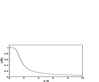
Figure 1: Reflection coefficient $|\gamma(kR)|$ as a function of $kR$ for the shear boundary condition (20) for weak, monochromatic quadrupolar waves with wave number $k$ and odd parity. The reflection coefficient is of order unity for small $kR$ and decays as $(kR)^{-1}$ for large $kR$.

V.3 Numerical tests

An ideal boundary condition would produce a solution that is identical (within the computational domain) to the corresponding solution on an unbounded domain. This principle was used in [10] to assess the numerical performance of various boundary conditions. First, a reference solution is computed on a very large computational domain. Next, the domain is truncated at a smaller distance where the boundary conditions are imposed. The reference domain is chosen large enough such that its boundary remains out of causal contact with the smaller domain for as long as we evolve. Finally, the solution on the smaller domain is compared with the reference solution, measuring the spurious reflections and constraint violations caused by the boundary conditions.

Here we use the same test problem as in [10]. The initial data are taken to be a Schwarzschild black hole of mass $M$ in Kerr-Schild coordinates with an outgoing odd-parity quadrupolar gravitational wave perturbation (satisfying the full nonlinear constraint equations). The perturbation is centered about a radius $r_{0}=5M$ initially and its dominant wavelength is $\lambda\approx 4M$.

These initial data are evolved on a spherical shell extending from $r=1.9M$ (just inside the horizon; no boundary conditions are needed here) out to $R=961.9M$ for the reference solution and to $R=41.9M$ for the truncated domain. The gauge source functions $H_{a}$ are chosen initially such that the time derivatives of the lapse and shift vanish, see Eqs. (10,11). This value of $H_{a}$ is then frozen in time.

A first order formulation (in both space and time) of the generalized harmonic Einstein equations is used as described in [4]. Our numerical implementation employs the Caltech-Cornell Spectral Einstein Code (SpEC), which is based on a pseudospectral collocation method. We refer the reader to appendix A of [10] for details on the numerical method, the test problem, and the various diagnostic quantities discussed below.

Four different sets of boundary conditions are compared,

1. the first order conditions (22)–(28), which include the vanishing shear condition (25),

2. the original Kreiss-Winicour [5] boundary conditions, which replace Eq. (25) with

   $$D_{lmm}\;\hat{=}\;q_{2}^{\prime}\,,$$ (101)

   and are otherwise identical to the previous set,

3. the second order constraint-preserving boundary conditions with $\Psi_{0}$ freezing, Eqs. (33)–(39),

4. the same as the previous set but with the first order gauge boundary conditions (22)–(24) instead of the second order ones (33)–(35); these are the boundary conditions used in [4, 9, 10].

Our implementation of the gauge boundary conditions differs from Eqs. (22)–(24) or (33)–(35) by terms of lower derivative order, which were found experimentally to slightly reduce reflections from the outer boundary in the components $l^{a}h_{ab}$ of the metric. Such non-principal terms do not affect the well posedness results of Sec. IV.

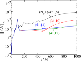
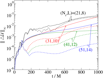
Figure 2: Difference $\Delta\mathcal{U}$ with respect to the reference solution for four different resolutions $(N_{r},L)$. Left: 1. vanishing shear (solid) vs. 2. Kreiss-Winicour (dotted) boundary conditions, right: 3. second order boundary conditions (solid) vs. 4. second order boundary conditions with first order gauge boundary conditions (dotted).

Fig. 2 shows the $L^{\infty}$ norm of the difference $\Delta\mathcal{U}$ of the solution on the truncated domain with respect to the reference solution as a function of time. This quantity is obtained by taking a tensor norm of the differences in the metric and its first derivatives at each point [10]. We normalize $\Delta\mathcal{U}$ by the analogous difference of the perturbed initial data with respect to the unperturbed data. The results for both versions of the first order boundary conditions are very similar. A first peak arises when the reflection from the outer boundary reaches the center, where its amplitude assumes its maximum because of the spherical geometry. For the second order boundary conditions, the peak is smaller by about two orders of magnitude. For the second order boundary conditions with first order gauge boundary conditions, $\Delta\mathcal{U}$ appears to converge away even for the higher resolutions at late times, unlike for the first order conditions. Unfortunately, this is not the case for the second order gauge boundary conditions. For those, $\Delta\mathcal{U}$ grows at late times at a rate that does not appear to depend on resolution in a monotonous way. A closer look at the data indicates that this growth only affects the $L=1,2$ spherical harmonic basis functions. We suspect that this is a numerical problem related to spectral filtering (cf. [27]); so far we have not been able to cure it. Note that $\Delta\mathcal{U}$ is a gauge-dependent quantity because the difference norm includes the entire spacetime metric. In fact, as we shall see below, inspection of the errors in the constraints and in the Newman-Penrose scalar $\Psi_{4}$ (which can be viewed as an approximation to the outgoing gravitational radiation) suggests that the blow-up is a pure gauge effect.

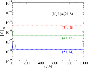
Figure 3: Constraint violations $\mathcal{C}$ for four different resolutions $(N_{r},L)$. Left: 1. vanishing shear (solid) vs. 2. Kreiss-Winicour (dotted) boundary conditions, right: 3. second order boundary conditions (solid) vs. 4. second order boundary conditions with first order gauge boundary conditions (dotted).

The violations of the constraints are shown in Fig. 3. The quantity $\mathcal{C}$ is a tensor norm including the harmonic constraints (2) as well as the additional constraints arising from the first order reduction of [4]. We normalize $\mathcal{C}$ by the second derivatives of the metric so that $\mathcal{C}\sim 1$ means that the constraints are not satisfied at all. The constraint violations converge away with increasing resolution for all the boundary conditions. This is what we expect because all the boundary conditions we considered are constraint-preserving.

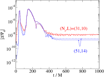
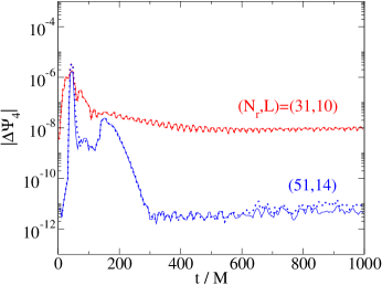
Figure 4: Difference of $\Psi_{4}$ with respect to the reference solution for two different resolutions. Left: 1. vanishing shear (solid) vs. 2. Kreiss-Winicour (dotted) boundary conditions, right: 3. second order boundary conditions (solid) vs. 4. second order boundary conditions with first order gauge boundary conditions (dotted).

One of the main objectives of numerical relativity is the computation of the gravitational radiation emitted by a compact source. Hence it is important to evaluate how the boundary conditions affect the accuracy of the extracted waveform. To this end, we compute the Newman-Penrose scalar $\Psi_{4}$ on an extraction sphere close to the outer boundary (at $R_{\mathrm{ex}}=40M$). The tetrad we use agrees with the one given in Eqs. (13)–(14) when evaluated for the background spacetime (see [10] for details). Strictly speaking, $\Psi_{4}$ only has a gauge-invariant meaning in the limit as future null infinity is approached but since our computational domain does not extend to infinity we can only evaluate $\Psi_{4}$ at a finite radius. However, $\Psi_{4}$ is gauge-invariant with respect to infinitesimal coordinate transformations and tetrad rotations on a Schwarzschild background, so errors in $\Psi_{4}$ due to gauge ambiguities should be very small. Fig. 4 shows the difference of $\Psi_{4}$ with respect to the same quantity obtained from the reference solution at the same location. We normalize $|\Delta\Psi_{4}|$ by the maximum in time of $|\Psi_{4}|$ at the extraction radius. Again, both versions of the first order boundary conditions show very similar numerical performance. Clearly visible is a first peak arising when the outgoing wave passes through the extraction sphere. Some of it is reflected off the boundary and excites the black hole, which then emits quasinormal mode radiation of exponentially decaying amplitude–a feature also visible in Fig. 4. The reflections are much smaller for (both versions of) the second order boundary conditions (about an order of magnitude at the first peak and two–three orders of magnitude later on). Unlike for the first order conditions, their $|\Delta\Psi_{4}|$ decreases with increasing resolution, at least at late times.

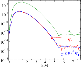
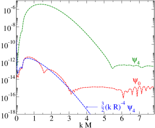
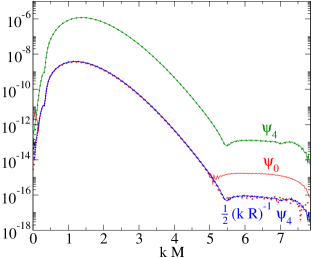
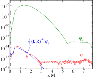
Figure 5: Comparison of the time Fourier transform of the measured $\Psi_{0}(t)$ (extracted $1.9M$ in from the outer boundary) with the predicted value using the reflection coefficients derived in Sec. V.2 and in [11]. Left: 1. vanishing shear (solid) vs. 2. Kreiss-Winicour (dotted) boundary conditions, right: 3. second order boundary conditions (solid) vs. 4. second order boundary conditions with first order gauge boundary conditions (dotted). Top: outer boundary radius $R=41.9M$, bottom: $R=121.9M$.

Finally we estimate the reflection coefficients for the various boundary conditions numerically and compare with the analytical predictions. As a consequence of the results of Ref. [11], the reflection coefficient can be approximated by forming the ratio of the Newman-Penrose scalars $\Psi_{0}$ and $\Psi_{4}$ at the outer boundary,

$$|\gamma(kR)|=\frac{|\Psi_{0}|}{|\Psi_{4}|}+\mathcal{O}(kR)^{-1},$$ (102)

where $k$ is the wavenumber and $R$ is the boundary radius. For the vanishing shear boundary conditions (25), we found in Sec. V.2

$$|\gamma(kR)|=\textstyle\frac{1}{2}(kR)^{-1}+\mathcal{O}(kR)^{-2},$$ (103)

whereas for the freezing-$\Psi_{0}$ condition (36), we have the much smaller reflection coefficient [11]

$$|\gamma(kR)|=\textstyle\frac{3}{2}(kR)^{-4}+\mathcal{O}(kR)^{-5}.$$ (104)

In Fig. 5, we compare the measured $\Psi_{0}$ with the predicted value obtained from Eq. (102), using the measured $\Psi_{4}$ and the above analytical expressions for the reflection coefficients. A Fourier transform in time has been taken in order to obtain plots vs. wavenumber $k$. The agreement is rather good, roughly at the expected level of accuracy $\mathcal{O}(kR)^{-1}$. The leveling off of the numerical $\Psi_{0}$ for large $k$ is likely to be caused by numerical roundoff error (note the magnitude of $\Psi_{0}$ at large $k$). The plots also indicate that the reflection coefficients are virtually the same for both versions of the second-order boundary conditions (as expected since they only differ in the gauge boundary conditions), and that the reflection coefficient of the original Kreiss-Winicour boundary conditions agrees with that of our vanishing shear conditions.

Summarizing, both versions of the first order conditions (those including the vanishing shear condition (25) and the original Kreiss-Winicour conditions) performed very similarly in our numerical test. In contrast, the second order conditions caused substantially less spurious reflections from the outer boundary.

VI Conclusions

In this paper, we have derived various sets of absorbing and constraint-preserving boundary conditions for the Einstein equations in the generalized harmonic gauge. We divided them into first, second and higher order boundary conditions where the order refers to the highest number of derivatives of the metric fields appearing in the boundary conditions. The first order boundary conditions are a generalization of the conditions considered by Kreiss and Winicour [5] and specify the shear of the outgoing null congruence associated with the two-dimensional cross sections of the boundary surface. Our second order conditions enable one to fix the Weyl scalar $\Psi_{0}$ at the boundary. Although there is a gauge ambiguity in the definition of $\Psi_{0}$ at finite radius, these conditions allow, in some sense, control of the incoming gravitational radiation. This is important for simulations aimed at the far-field extraction of gravitational waves emitted from compact astrophysical sources. Furthermore, we could for example study the critical collapse of gravitational waves by starting with Minkowski spacetime and injecting pulses of gravitational radiation through the outer boundary with different amplitudes [26, 4]. Finally, we have considered higher order boundary conditions which comprise the hierarchy of absorbing boundary conditions ${\cal B}_{L}$ and ${\cal C}_{L}$ discussed in [11, 12]. As was shown in these references, ${\cal B}_{L}$ and ${\cal C}_{L}$ yield fewer and fewer spurious reflections of gravitational radiation as $L$ is increased.

In Sec. IV, we have analyzed the well posedness of the IBVPs resulting from our different boundary conditions. In order to do so, we considered high-frequency perturbations of a given smooth background solution in which case the problem reduces to a system of ten decoupled wave equations with boundary conditions on a frozen background spacetime. By means of a suitable coordinate transformation, we have reduced the background metric to the flat metric, with the exception of the component of the shift normal to the boundary. Using the technique of Kreiss and Winicour [5] which is based on a reduction to a pseudo-differential first order system and the construction of smooth symmetrizer, we then have shown that the resulting IBVPs are well posed in the high-frequency limit. In view of the theory of pseudo-differential operators [24] and the fact that we obtain estimates for derivatives of arbirtrary order it is expected that the full nonlinear problem is well posed as well. Our results thus generalize the work of Ref. [5] to non-trivial shifts and boundary conditions of arbitrarily high order. They also strengthen the result of Ref. [9], where boundary stability but not well posedness was proved for a first order version of the generalized harmonic Einstein equations derived in [4]. We remark that our results imply well posedness of such first order formulations provided that the evolution system of the additional constraints related to the first order reduction (supplemented with suitable constraint-preserving boundary conditions) is well posed. For a recent proof of well posedness for the first order boundary conditions which is based on integration by parts, and which does not require the pseudo-differential calculus, see [41].

In order to study the quality of the different boundary conditions considered in this paper, we have computed the amount of spurious gravitational radiation reflected off the boundary in the high-frequency approximation in Sec. V. We have shown that fewer and fewer reflections are present if the order of the boundary conditions is increased. In addition, we have generalized that analysis without the high frequency approximation for odd-parity linear gravitational waves with wavenumber $k$ propagating on the asymptotic region of a Schwarzschild background. For the case of a spherical outer boundary of areal radius $R$ with the shear boundary condition the reflection coefficient has been found to scale only as $(kR)^{-1}$ for large $kR$ which is much slower than the $(kR)^{-4}$ decay calculated for the freezing-$\Psi_{0}$ boundary condition [11]. Finally, we have performed numerical tests of some of our boundary conditions similar to the ones presented in [10]. The initial data were taken to be a Schwarzschild black hole with an outgoing odd-parity quadrupolar gravitational wave perturbation. The first order boundary conditions (with our modified vanishing-shear condition) performed very similarly to the original conditions considered in [5]. In contrast, as expected from the analytic considerations, the second order conditions caused substantially less spurious reflections from the outer boundary. A numerical implementation of the higher order boundary conditions is beyond the scope of this article and will be presented in future work.

- [1] D. Givoli. Non-reflecting boundary conditions. J. Comp. Phys., 94:1–29, 1991.
- [2] Bela Szilagyi and Jeffrey Winicour. Well-posed initial-boundary evolution in general relativity. Phys. Rev., D68:041501, 2003.
- [3] Bela Szilagyi, Bernd G. Schmidt, and Jeffrey Winicour. Boundary conditions in linearized harmonic gravity. Phys. Rev., D65:064015, 2002.
- [4] L. Lindblom, M. A. Scheel, L. E. Kidder, R. Owen, and O. Rinne. A new generalized harmonic evolution system. Class. Quant. Grav., 23:S447– S462, 2006.
- [5] H. O. Kreiss and J. Winicour. Problems which are well-posed in a generalized sense with applications to the Einstein equations. Class. Quant. Grav., 23:S405–S420, 2006.
- [6] Maria C. Babiuc, Bela Szilagyi, and Jeffrey Winicour. Harmonic initial-boundary evolution in general relativity. Phys. Rev., D73:064017, 2006.
- [7] Mohammad Motamed, M. Babiuc, B. Szilagyi, and H-O. Kreiss. Finite difference schemes for second order systems describing black holes. Phys. Rev., D73:124008, 2006.
- [8] M. C. Babiuc, H. O. Kreiss, and Jeffrey Winicour. Constraint-preserving Sommerfeld conditions for the harmonic Einstein equations. Phys. Rev., D75:044002, 2007.
- [9] Oliver Rinne. Stable radiation-controlling boundary conditions for the generalized harmonic Einstein equations. Class. Quant. Grav., 23:6275–6300, 2006.
- [10] Oliver Rinne, Lee Lindblom, and Mark A. Scheel. Testing outer boundary treatments for the Einstein equations. Class. Quant. Grav., 24:4053–4078, 2007.
- [11] Luisa T. Buchman and Olivier C. A. Sarbach. Towards absorbing outer boundaries in general relativity. Class. Quant. Grav., 23:6709–6744, 2006.
- [12] Luisa T. Buchman and Olivier C. A. Sarbach. Improved outer boundary conditions for Einstein’s field equations. Class. Quant. Grav., 24:S307–S326, 2007.
- [13] H. Friedrich and G. Nagy. The initial boundary value problem for Einstein’s vacuum field equations. Comm. Math. Phys., 201:619–655, 1999.
- [14] K.O. Friedrichs. Symmetric positive linear differential equations. Commun. Pure Appl. Math., 11:333–418, 1958.
- [15] P.D. Lax and R.S. Phillips. Local boundary conditions for dissipative symmetric linear differential operators. Commun. Pure Appl. Math., 13:427–455, 1960.
- [16] P. Secchi. Well-posedness of characteristic symmetric hyperbolic systems. Arch. Rat. Mech. Anal., 134:155–197, 1996.
- [17] Gioel Calabrese, Jorge Pullin, Olivier Sarbach, Manuel Tiglio, and Oscar Reula. Well posed constraint-preserving boundary conditions for the linearized Einstein equations. Commun. Math. Phys., 240:377–395, 2003.
- [18] Carsten Gundlach and Jose M. Mart\a’ın-Garc\a’ıa. Symmetric hyperbolicity and consistent boundary conditions for second-order Einstein equations. Phys. Rev., D70:044032, 2004.
- [19] Gabriel Nagy and Olivier Sarbach. A minimization problem for the lapse and the initial- boundary value problem for Einstein’s field equations. Class. Quant. Grav., 23:S477–S504, 2006.
- [20] H. O. Kreiss and J. Lorenz. Initial-boundary value problems and the Navier-Stokes equations. Academic Press, San Diego, 1989.
- [21] H.O. Kreiss. Initial boundary value problems for hyperbolic systems. Commun. Pure Appl. Math., 23:277–298, 1970.
- [22] J.M. Stewart. The Cauchy problem and the initial boundary value problem in numerical relativity. Class. Quantum Grav., 15:2865–2889, 1998.
- [23] A. Majda and S. Osher. Initial-boundary value problems for hyperbolic equations with uniformly characteristic boundary. Commun. Pure Appl. Math., 28:607–675, 1975.
- [24] M.E. Taylor. Partial differential equations II, Qualitative Studies of Linear Equations. Springer, 1999.
- [25] James M. Bardeen and L. T. Buchman. Numerical tests of evolution systems, gauge conditions, and boundary conditions for 1d colliding gravitational plane waves. Phys. Rev., D65:064037, 2002.
- [26] Olivier Sarbach and Manuel Tiglio. Boundary conditions for Einstein’s field equations: Analytical and numerical analysis. J. Hyperbol. Diff. Equat., 2:839, 2005.
- [27] L.E. Kidder, L. Lindblom, M.A. Scheel, L.T. Buchman, and H.P. Pfeiffer. Boundary conditions for the Einstein evolution system. Phys. Rev. D, 71:064020, 2005.
- [28] H. Friedrich. On the hyperbolicity of Einstein’s and other gauge field equations. Comm. Math. Phys., 100:525–543, 1985.
- [29] H. Friedrich. Hyperbolic reductions for Einstein’s equations. Class. Quantum Grav., 13:1451–1469, 1996.
- [30] L. Andersson and V. Moncrief. Elliptic-hyperbolic systems and the Einstein equations. Annales Henri Poincar\a’e, 4:1–34, 2003.
- [31] Frans Pretorius. Numerical relativity using a generalized harmonic decomposition. Class. Quant. Grav., 22:425–452, 2005.
- [32] A. E. Fischer and J. E. Marsden. The Einstein evolution equations as a first-order quasi-linear symmetric hyperbolic system, I. Comm. Math. Phys., 28:1–38, 1972.
- [33] Y. Foures-Bruhat. Théorème d’éxistence pour certains systèmes d’équations aux dérivées partielles non linéaires. Acta Math., 88:141–225, 1952.
- [34] B. Gustafsson, H.O. Kreiss, and J. Oliger. Time dependent problems and difference methods. Wiley, New York, 1995.
- [35] Oscar Reula and Olivier Sarbach. A model problem for the initial-boundary value formulation of Einstein’s field equations. J. Hyperbol. Diff. Equat., 2:397–435, 2005.
- [36] B. Engquist and A. Majda. Absorbing boundary conditions for the numerical simulation of waves. Math. Comp., 31:629–651, 1977.
- [37] U.H. Gerlach and U.K. Sengupta. Gauge-invariant perturbations on most general spherically symmetric space-times. Phys. Rev. D, 19:2268–2272, 1979.
- [38] T. Regge and J. Wheeler. Stability of a Schwarzschild singularity. Phys. Rev., 108:1063–1069, 1957.
- [39] Olivier Sarbach, Markus Heusler, and Othmar Brodbeck. Perturbation theory for self-gravitating gauge fields: The odd-parity sector. Phys. Rev., D62:084001, 2000.
- [40] Olivier Sarbach and Manuel Tiglio. Gauge invariant perturbations of Schwarzschild black holes in horizon-penetrating coordinates. Phys. Rev., D64:084016, 2001.
- [41] H. O. Kreiss, O. Reula, O. Sarbach, and J. Winicour. Well-posed initial-boundary value problem for the harmonic Einstein equations using energy estimates. Class. Quant. Grav., 2007. To appear.