Distributed Compression and Multiparty Squashed Entanglement

Abstract

We study a protocol in which many parties use quantum communication to transfer a shared state to a receiver without communicating with each other. This protocol is a multiparty version of the fully quantum Slepian-Wolf protocol for two senders and arises through the repeated application of the two-sender protocol. We describe bounds on the achievable rate region for the distributed compression problem. The inner bound arises by expressing the achievable rate region for our protocol in terms of its vertices and extreme rays and, equivalently, in terms of facet inequalities. We also prove an outer bound on all possible rates for distributed compression based on the multiparty squashed entanglement, a measure of multiparty entanglement.

I Introduction

Quantum information theory studies the interconversion of information resources like quantum channels, states and entanglement for the purpose of accomplishing communication tasks BBPS ; DHW04 ; DHW05b ; FQSW . This approach is rendered possible by the substantial body of results characterizing quantum channels H98 ; SW97 ; BSST99 ; D03 and quantum communication resources like entanglement B96 ; DW05 ; PV07 .

In classical information theory, distributed compression is the search for the optimal rates at which two parties Alice and Bob can compress and transmit information faithfully to a third party Charlie. If the senders are allowed to communicate among themselves then they can obviously use the correlations between their sources to achieve better rates. The more interesting problem is to ask what rates can be achieved if no communication is allowed between the senders. The classical version of this problem was solved by Slepian and Wolf SW73 . The quantum version of this problem was first approached in ADHW04 ; HOW05 and more recently in FQSW , which describes the Fully Quantum Slepian-Wolf (FQSW) protocol and partially solves the distributed compression problem for two senders.

In this paper we generalize the results of the FQSW protocol to a multiparty scenario where $m$ senders, Alice 1 through Alice $m$, send quantum information to a single receiver, Charlie. We exhibit a set of achievable rates as well as an outer bound on the possible rates based on a new measure of multiparty entanglement that generalizes squashed entanglement CW04 . Our protocol is optimal for input states that have zero squashed entanglement, notably separable states.

The multiparty squashed entanglement is interesting in its own right, and we develop a number of its properties in the paper. (It was also found independently by Yang et al. and described in a recent paper multisquash .) While there exist several measures for bipartite entanglement with useful properties and applications BBPS ; HHT ; Ra99 ; VP98 , the theory of multiparty entanglement, despite considerable effort LSSW ; DCT99 ; CKW00 ; BPRST99 , remains comparatively undeveloped. Multiparty entanglement is fundamentally more complicated because it cannot be described by a single number even for pure states. We can, however, define useful entanglement measures for particular applications, and the multiparty squashed entanglement seems well-suited to application in the distributed compression problem.

The structure of the paper is as follows. In section II we describe the quantum distributed compression problem and present our protocol. Our results are twofold. In Theorem II.1 we give the formula for the achievable rate region using this protocol and in Theorem II.2 we provide a bound on the best possible rates for any protocol. The proof of Theorem II.1 is in section III. The proof of Theorem II.2 is given in section VI but before we get to it we need to introduce and describe the properties of the multiparty information quantity in section IV and multiparty squashed entanglement in section V.

Notation:    We will denote quantum systems as $A,B,R$ and the corresponding Hilbert spaces ${\cal H}^{A},{\cal H}^{B},{\cal H}^{R}$ with respective dimensions $d_{A},d_{B},d_{R}$. We denote pure states of the system $A$ by a ket $\left|\varphi\right\rangle^{A}$ and the corresponding density matrices as $\varphi^{A}=|\varphi\rangle\!\langle\varphi|^{A}$. We denote by $H(A)_{\rho}=-\textup{Tr}\left(\rho^{A}\log\rho^{A}\right)$ the von Neumann entropy of the state $\rho^{A}$. For a bipartite state $\sigma^{AB}$ we define the conditional entropy $H(A|B)_{\sigma}=H(AB)_{\sigma}-H(B)_{\sigma}$ and the mutual information $I(A;B)_{\sigma}=H(A)_{\sigma}+H(B)_{\sigma}-H(AB)_{\sigma}$. The trace distance between states $\sigma$ and $\rho$ is $\|\sigma-\rho\|_{1}=\mathrm{Tr}|\sigma-\rho|$ where $|X|=\sqrt{X^{\dagger}X}$. The fidelity is defined to be $F(\sigma,\rho)=\mathrm{Tr}\left(\sqrt{\sqrt{\rho}\sigma\sqrt{\rho}}\right)^{2}$. Two states that are very similar have fidelity close to 1 whereas states with little similarity will have low fidelity. Throughout this paper, logarithms and exponents are taken base two unless otherwise specified.

II Multiparty Distributed Compression

Distributed compression of classical information involves many parties collaboratively encoding their sources $X_{1},X_{2}\cdots X_{m}$ and sending the information to a common receiver C75 . In the quantum setting, the parties are given a quantum state $\varphi^{A_{1}A_{2}\cdots A_{m}}\in{\cal H}^{A_{1}A_{2}\cdots A_{m}}$ and are asked to individually compress their shares of the state and transfer them to the receiver while sending as few qubits as possible ADHW04 . The objective is to successfully transmit the quantum information stored in the $A$ systems, meaning any entanglement with an external reference system, to the receiver. No communication between the senders is allowed and, unlike HOW05 , in this paper there is no classical communication between the senders and the receiver.

In our analysis, we work in the case where we have many copies of the input state, so that the goal is to send shares of the purification $\left|\psi\right\rangle^{A_{1}A_{2}\cdots\!A_{m}R}=(\left|\varphi\right\rangle^{A_{1}A_{2}\cdots\!A_{m}R})^{\otimes n}$, where the $A_{i}$’s denote the $m$ different systems and $R$ denotes the reference system, which does not participate in the protocol. Notice that we use $A_{i}$ to denote both the individual system associated with state $\varphi$ as well the $n$-copy version associated with $\psi$; the meaning should be clear from the context. We also use the shorthand notation $A=A_{1}A_{2}\cdots\!A_{m}$ to denote all the senders.

The objective, as we have mentioned, is for the participants to transfer their $R$-entanglement to a third party Charlie as illustrated in Figure 1. Note that any other type of correlation the $A$ systems could have with an external subsystem is automatically preserved in this case, which implies for example that if $\varphi$ were written as a convex combination $\varphi=\sum_{i}p_{i}\varphi_{i}$ then a successful protocol would automatically send the $\varphi_{i}$ with high fidelity on average EntFid .

Figure 1: Pictorial representation of the quantum correlations between the systems at three stages of the protocol. Originally the state $\left|\psi\right\rangle$ is shared between $A_{1}A_{2}\cdots A_{m}$ and $R$. The middle picture shows the protocol in progress. Finally, all systems are received by Charlie and $\left|\psi\right\rangle$ is now shared between Charlie’s systems $\widehat{A}_{1}\widehat{A}_{2}\cdots\widehat{A}_{m}$ and $R$.

An equivalent way of thinking about quantum distributed compression is to say that the participants are attempting to decouple their systems from the reference $R$ solely by sending quantum information to Charlie. Indeed, if we assume that originally $R$ is the purification of $A_{1}A_{2}\cdots A_{m}$, and at the end of the protocol there are no correlations between the remnant $W$ systems (see Figure 1) and $R$, then the purification of $R$ must have been transferred to Charlie’s laboratory since none of the original information was discarded.

To perform the distributed compression task, each of the senders independently encodes her share before sending part of it to Charlie. The encoding operations are modeled by quantum operations, that is, completely positive trace-preserving (CPTP) maps $E_{i}$ with outputs $C_{i}$ of dimension $2^{nQ_{i}}$. Once Charlie receives the systems that were sent to him, he will apply a decoding CPTP map $D$ with output system $\widehat{A}=\widehat{A}_{1}\widehat{A}_{2}\ldots\widehat{A}_{m}$ isomorphic to the original $A=A_{1}A_{2}\ldots A_{m}$.

Definition II.1 (The rate region).

We say that a rate tuple $\vec{Q}=(Q_{1},Q_{2},\ldots,Q_{m})$ is achievable if for all $\epsilon>0$ there exists $N(\epsilon)$ such that for all $n\geq N(\epsilon)$ there exist $n$-dependent maps $(E_{1},E_{2},\ldots,E_{m},D)$ with domains and ranges as in the previous paragraph for which the fidelity between the original state, $\left|\psi\right\rangle^{A^{n}R^{n}}=\left(\left|\varphi\right\rangle^{A_{1}A_{2}\cdots\!A_{m}R}\right)^{\otimes n}$, and the final state, ${\sigma}^{\widehat{A}_{1}\widehat{A}_{2}\ldots\widehat{A}_{m}R}={\sigma}^{\widehat{A}^{n}R^{n}}$, satisfies

$$F\left(\left|\psi\right\rangle^{A^{n}R^{n}}\!,\ {\sigma}^{\widehat{A}^{n}R^{n}}\right)=\phantom{.}^{\widehat{A}^{n}R^{n}}\!\!\left\langle\psi\right|(D\circ(E_{1}\otimes\cdots\otimes E_{m}))(\psi^{A^{n}R^{n}})\left|\psi\right\rangle^{\widehat{A}^{n}R^{n}}\geq 1-\epsilon.$$ (1)

We call the closure of the set of achievable rate tuples the rate region.

At this point it is illustrative to review the results of the two-party state transfer protocol FQSW , which form a key building block for the multiparty distributed compression protocol presented in section II.2.

II.1 The FQSW protocol

The fully quantum Slepian-Wolf protocol FQSW describes a procedure for simultaneous quantum state transfer and entanglement distillation. This communication task can be used as a building block for nearly all the other protocols of quantum information theory DHW04 , yet despite its powerful applications it is fairly simple to implement.

Consider a setup where the state $\left|\psi\right\rangle^{ABR}=\left(\left|\varphi\right\rangle^{ABR}\right)^{\otimes n}$ is shared between Alice, Bob and a reference system $R$. The FQSW protocol describes a procedure for Alice to transfer her $R$-entanglement to Bob while at the same time generating ebits with him. Alice can accomplish this by encoding and sending part of her system, denoted $A_{1}$, to Bob. The state after the protocol can approximately be written as $\left|\Phi\right\rangle^{A_{2}\widetilde{B}}(\left|\varphi\right\rangle^{R\widehat{B}})^{\otimes n}$, where the systems $\widetilde{B}$ and $\widehat{B}$ are held in Bob’s lab while $A_{2}$ remains with Alice. The state $\left|\Phi\right\rangle^{A_{2}\widetilde{B}}$ is a maximally entangled state shared between Alice and Bob, a handy side-product which can be used to build more advanced protocols DH06 ; DY06 . Figure 2 illustrates the entanglement structure before and after the protocol.

Figure 2: Diagram representing the $ABR$ correlations before and after the FQSW protocol. Alice manages to decouple completely from the reference $R$. The $\widehat{B}$ system is isomorphic to $AB$.

The protocol, represented graphically in Figure 3, consists of the following steps:

1. Alice performs Schumacher compression on her system $A$ to obtain the output system $A^{S}$.

2. Alice then applies a random unitary $U_{A}$ to $A^{S}$.

3. Next, she splits her system into two parts: $A_{1}A_{2}=A^{S}$ with $d_{A_{1}}=2^{nQ_{A}}$ and

   $$Q_{A}>\frac{1}{2}I(A;R)_{\varphi}.$$ (2)

   She sends the system $A_{1}$ to Bob.

4. Bob, in turn, performs a decoding operation $V_{B}^{{A_{1}B}\to\widehat{B}\widetilde{B}}$ which splits his system into a $\widehat{B}$ part purifying $R$ and a $\widetilde{B}$ part which is fully entangled with Alice.

Figure 3: A circuit diagram that shows the Schumacher compression and unitary encoding done by Alice and the decoding done by Bob.

The best way to understand the mechanism behind this protocol is by thinking about destroying correlations. If, at the end of the protocol, Alice’s system $A_{2}$ is nearly decoupled from the reference in the sense that $\sigma^{A_{2}R}\approx\sigma^{A_{2}}\otimes\sigma^{R}$, then Alice must have succeeded in sending her $R$ entanglement to Bob because it is Bob alone who then holds the $R$ purification. We can therefore guess the lower bound on how many qubits Alice will have to send before she can decouple from the reference. Originally, Alice and R share $I(A;R)_{\varphi}$ bits of information per copy of $\left|\varphi\right\rangle^{ABR}$. Since one qubit can carry away at most two bits of quantum mutual information, this means that the minimum rate at which Alice must send qubits to Bob is

$$Q_{A}>\frac{1}{2}I(A;R)_{\varphi}.$$ (3)

It is shown in FQSW that this rate is achievable in the limit of many copies of the state. Therefore the FQSW protocol is optimal for the state transfer task.

II.2 The multiparty FQSW protocol

Like the original FQSW protocol, the multiparty version relies on Schumacher compression and the mixing effect of random unitary operations for the encoding. The only additional ingredient is an agreed upon permutation of the participants. The temporal order in which the participants will perform their encoding is of no importance. However, the permutation determines how much information each participant is to send to Charlie.

For each permutation $\pi$ of the participants, the protocol consists of the following steps:

1. Each Alice-$i$ performs Schumacher compression on her system $A_{i}$ reducing its effective size to the entropy bound of roughly $H(A_{i})$ qubits per copy of the state.

2. Each participant applies a known, pre-selected random unitary to the compressed system.

3. Participant $i$ sends to Charlie a system $C_{i}$ of dimension $2^{nQ_{i}}$ where

   $$Q_{i}>\frac{1}{2}I(A_{i};A_{\mathcal{K}_{i}}R)_{\varphi}$$ (4)

   where $\mathcal{K}_{i}=\{\pi\!(j):j>\pi^{\mbox{-}1}(i)\}$ is the set of participants who come after participant $i$ according to the permutation.

4. Charlie applies a decoding operation $D$ consisting of the composition of the decoding maps $D_{\pi\!(m)}\circ\cdots\circ D_{\pi\!(2)}\circ D_{\pi\!(1)}$ defined by the individual FQSW steps in order to recover $\sigma^{\widehat{A}_{1}\widehat{A}_{2}\ldots\widehat{A}_{m}}$ nearly identical to the original $\psi^{A_{1}A_{2}\cdots\!A_{m}}$ and purifying $R$.

II.3 Statement of Results

This subsection contains our two main theorems about multiparty distributed compression. In Theorem II.1 we give the formula for the set of achievable rates using the multiparty FQSW protocol (sufficient conditions). Then, in Theorem II.2 we specify another set of inequalities for the rates $Q_{i}$ which must be true for any distributed compression protocol (necessary conditions). In what follows, we consistently use $\mathcal{K}\subseteq\{1,2,\ldots m\}$ to denote any subset of the senders in the protocol.

Theorem II.1.

Let $\left|\varphi\right\rangle^{A_{1}A_{2}\cdots A_{m}R}$ be a pure state. If the inequality

$$\sum_{k\in\mathcal{K}}Q_{k}\geq\frac{1}{2}\left[\sum_{k\in\mathcal{K}}\!\left[H(A_{k})_{\varphi}\right]+H(R)_{\varphi}-H(RA_{\mathcal{K}})_{\varphi}\right]$$ (5)

holds for all $\mathcal{K}\subseteq\{1,2,\ldots,m\}$, then the rate tuple $(Q_{1},Q_{2},\cdots,Q_{m})$ is achievable for distributed compression of the $A_{i}$ systems.

Because Theorem II.1 expresses a set of sufficient conditions for the protocol to succeed, we say that these rates are contained in the rate region. The proof is given in the next section.

In the $m$-dimensional space of rate tuples $(Q_{1},Q_{2},\cdots,Q_{m})\in{{\mathbb{R}}}^{m}$, the inequalities (5) define a convex polyhedron poly whose facets are given by the corresponding hyperplanes, as illustrated in Figure 4.

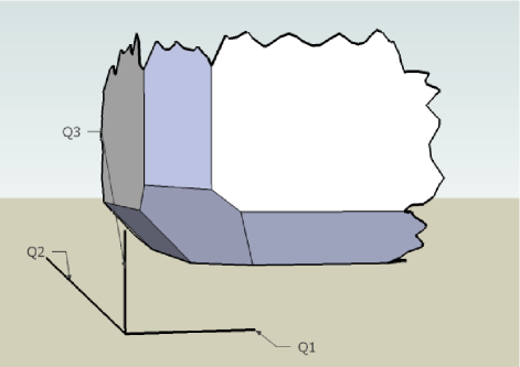
Figure 4: Sketch of the rate region for the multiparty FQSW protocol for three senders.

In order to characterize the rate region further we also derive an outer bound which all rate tuples must satisfy.

Theorem II.2.

Let $\left|\varphi\right\rangle^{A_{1}A_{2}\cdots A_{m}R}$ be a pure state input to a distributed compression protocol which achieves the rate tuple $(Q_{1},Q_{2},\ldots,Q_{m})$, then it must be true that

$$\sum_{k\in\mathcal{K}}Q_{k}\geq\frac{1}{2}\left[\sum_{k\in\mathcal{K}}\!\left[H(A_{k})_{\varphi}\right]+H(R)_{\varphi}-H(RA_{\mathcal{K}})_{\varphi}\right]-E_{\text{sq}}(A_{k_{1}};A_{k_{2}};\ldots;A_{k_{|\mathcal{K}|}})_{\varphi},$$ (6)

for all $\mathcal{K}\subseteq\{1,2,\ldots,m\}$, where $E_{\text{sq}}$ is the multiparty squashed entanglement.

The multiparty squashed entanglement, independently discovered in multisquash , is a measure of multipartite entanglement which generalizes the bipartite squashed entanglement of CW04 . Sections IV and V below define the quantity and investigate some of its properties. The proof of II.2 is given in section VI.

Notice that Theorems II.1 and II.2 both provide bounds of the same form and only differ by the presence of the $E_{\text{sq}}$ term. The rate region is squeezed somewhere between these two bounds as illustrated in Figure 5.

Figure 5: A two dimensional diagram showing the inner bound from Theorem II.1 and the outer bound from Theorem II.2. The boundary of the real rate region must lie somewhere in between.

For states which have zero squashed entanglement, the inner and outer bounds on the region coincide so that in those cases our protocol is an optimal solution to the multiparty distributed compression problem.

One can verify that when only two parties are involved ($m=2$), the inequalities in (5) reduce to the 2-party bounds in the original FQSW paper:

$$Q_{1} \geq\frac{1}{2}I({A_{1}};R),$$

$$Q_{2} \geq\frac{1}{2}I(A_{2};R),$$

$$Q_{1}+Q_{2} \geq\frac{1}{2}\left[H({A_{1}})+H({A_{2}})+H({A_{1}}{A_{2}})\right].$$

The family of inequalities (6) similarly reduce to the corresponding expressions in FQSW with the multiparty squashed entanglement being replaced by the original two-party squashed entanglement of CW04 .

III Proof of the Achievable Rates

The multiparty fully quantum Slepian-Wolf protocol can be constructed through the repeated application of the two-party FQSW protocol FQSW . In the multiparty case, however, the geometry of the rate region is more involved and some concepts from the theory of polyhedra poly prove helpful in giving it a precise characterization. Multiparty rate regions in information theory have previously appeared in C75 ; TH98 .

For every permutation $\pi\in S_{m}$ of the $m$ senders, there is a different rate tuple $\vec{q}_{\pi}=(Q_{1},Q_{2},\ldots,Q_{m})_{\pi}\in{{\mathbb{R}}}^{m}$ which is achievable in the limit of many copies of the state. By time-sharing we can achieve any rate that lies in the convex hull of these points. We will show that the rate region for an input state $\left|\varphi\right\rangle^{A_{1}\cdots A_{m}R}$ can equivalently be described by the set of inequalities from Theorem II.1, that is

$$\sum_{k\in\mathcal{K}}Q_{k}\geq\frac{1}{2}\left[\sum_{k\in\mathcal{K}}\!H(A_{k})_{\varphi}+H(R)_{\varphi}-H(RA_{\mathcal{K}})_{\varphi}\right]=:C_{\mathcal{K}}$$ (7)

where $\mathcal{K}\subseteq\{1,2,\ldots,m\}$ ranges over all subsets of participants and $C_{\mathcal{K}}$ is the name we give to the constant on the right hand side of the inequality. The proof of Theorem II.1 proceeds in two steps. First we show the set of rate tuples $\{\vec{q}_{\pi}\}$ is contained in the rate region and then we prove that the set of inequalities (7) is an equivalent description of the rates obtained by time sharing and resource wasting of the rates $\{\vec{q}_{\pi}\}$.

Consider the $m$-dimensional space of rate tuples $(Q_{1},\cdots,Q_{m})\in{{\mathbb{R}}}^{m}$. We begin by a formal definition of a corner point $\vec{q}_{\pi}$.

Definition III.1 (Corner point).

Let $\pi\in S_{m}$ be a permutations of the senders in the protocol. The corresponding rate tuple $q_{\pi}=(Q_{1},Q_{2},\ldots,Q_{m})$ is a corner point if

$$Q_{\pi\!(k)}=\frac{1}{2}I(A_{\pi\!(k)};A_{\pi\!(k+1)}\cdots A_{\pi\!(m)}R)$$ (8)

where the set $A_{\pi\!(k+1)}\cdots A_{\pi\!(m)}$ denotes all the systems which come after $k$ in the permutation $\pi$.

We define $\mathcal{Q}:=\{\vec{q}_{\pi}:\pi\in S_{m}\}$, the set of all corner points. Clearly, $|\mathcal{Q}|\leq m!$ but since some permutations might lead to the same rate tuple, the inequality may be strict.

Lemma III.2.

The set of corner points, $\mathcal{Q}=\{\vec{q}_{\pi}:\pi\in S_{m}\}$, is contained in the rate region.

Proof sketch for Lemma III.2.

We will now exhibit a protocol that achieves one such point. In order to simplify the notation, but without loss of generality, we choose the reversed-order permutation $\pi=(m,\ldots,2,1)$. This choice of permutation corresponds to Alice-$m$ sending her information first and Alice-$1$ sending last.

We will repeatedly use the FQSW protocol is order to send the $m$ systems to Charlie:

1. The first party Schumacher compresses her system $A_{m}$ and sends it to Charlie. She succeeds provided

   $$Q_{m}\geq\frac{1}{2}I(A_{m};A_{1}A_{2}\ldots A_{m-1}R)+\delta=H(A_{m})+\delta$$

   for any $\delta>0$. The above rate is dictated by the FQSW inequality (3) because we are facing the same type of problem except that the “reference” consists of $R$ as well as the remaining participants $A_{1}A_{2}\cdots A_{m-1}$. The fact that the formula reduces to $Q_{m}>H(A_{m})$ should also be expected since there are no correlations that the first participant can take advantage of; she is just performing Schumacher compression.

2. The second party also faces an instance of an FQSW problem. The task is to transmit the system $A_{m-1}$ to Charlie, who is now assumed to hold $A_{m}$. The purifying system consists of $A_{1}A_{2}\cdots A_{m-2}R$. According to inequality (3) the rate must be

   $$Q_{m-1}\geq\frac{1}{2}I(A_{m-1};A_{1}A_{2}\cdots A_{m-2}R)+\delta$$

   for any $\delta>0$.

3. The last person to be merging with Charlie will have a purifying system consisting of only $R$. Her transfer will be successful if

   $$Q_{1}\geq\frac{1}{2}I(A_{1};R)+\delta$$

   for any $\delta>0$.

On the receiving end of the protocol, Charlie will apply the decoding map $D$ consisting of the composition of the decoding maps $D_{1}\circ D_{2}\circ\cdots\circ D_{m}$ defined by the individual FQSW steps to recover the state $\sigma^{\widehat{A}_{1}\widehat{A}_{2}\cdots\widehat{A}_{m}}$, which will be such that the fidelity between $\left|\psi\right\rangle^{A^{n}R^{n}}$ and $\sigma^{\hat{A}^{n}R^{n}}$ is high, essentially by the triangle inequality. Finally, because we can make $\delta$ arbitrarily small, the rate tuple $(Q_{1},\cdots,Q_{m})$, with

$$Q_{k}=\frac{1}{2}I(A_{k};A_{1}\cdots A_{k\!-\!1}R),$$ (9)

must be contained in the rate region. The same argument applies for each permutation $\pi\in S_{m}$, leading to the conclusion that the full set $\mathcal{Q}$ is contained in the rate region. ∎

Each one of the corner points $\vec{q}_{\pi}$ can also be described by an equivalent set of equations involving sums of the rates.

Lemma III.3.

The rate tuple $(Q_{1},Q_{2},\ldots,Q_{m})$ is a corner point if and only if for some $\pi\in S_{m}$ and for all $l$ such that $1\leq l\leq m$,

$$\sum_{m-l+1\leq k\leq m}Q_{\pi\!(k)}=\frac{1}{2}\left[\sum_{m-l+1\leq k\leq m}\!\!\!\!\!\!\!\!\!H(A_{\pi\!(k)})+H(R)-H(A_{\pi\![m-l+1,m]}R)\right]=C_{\pi\![m-l+1,m]}$$ (10)

where $A_{\pi\![m-l+1,m]}:=A_{\pi\!(m-l+1)}A_{\pi\!(m-l+2)}\cdots A_{\pi\!(m)}$ denotes the last $l$ participants according to the permutation $\pi$.

Proof of Lemma III.3.

The proof follows trivially from Lemma III.2 by considering sums of the rates. If we again choose the permutation $\pi=(m,\ldots,2,1)$ for simplicity, we see that the sum of the rates of the last $l$ participants is

$$Q_{1}+\cdots+Q_{l} =\frac{1}{2}\bigg{[}I(A_{1};R)+I(A_{2};A_{1}R)+\cdots+I(A_{l};A_{1}\cdots A_{l-1}R)\bigg{]}$$

$$=\frac{1}{2}\bigg{[}\sum_{1\leq k\leq l}H(A_{k})+H(R)-H(A_{1}\cdots A_{l}R)\bigg{]}=C_{12\ldots l}.$$ (11)

A telescoping effect occurs and most of the inner terms cancel so we are left with a system of equations identical to (10). Moreover, this system is clearly solvable for the individual rates $Q_{k}$. The analogous simplification occurs for all other permutations. ∎

So far, we have shown that the set of corner points $\mathcal{Q}$ is contained in the rate region of the multiparty fully quantum Slepian-Wolf protocol. The convex hull of a set of points $\mathcal{Q}$ is defined to be

$$conv(\mathcal{Q}):=\left\{\vec{x}\in{{\mathbb{R}}}^{m}:\ \vec{x}=\sum\lambda_{i}\vec{q}_{i},\ \vec{q}_{i}\in\mathcal{Q},\ \lambda_{i}\geq 0,\ \sum\lambda_{i}=1\right\}.$$ (12)

Because of the possibility of time-sharing between the different corner points, the entire convex hull $conv(\mathcal{Q})$ must be achievable. Furthermore, by simply allowing any one of the senders to waste resources, we know that if a rate tuple $\vec{q}$ is achievable, then so is $\vec{q}+\vec{w}$ for any vector $\vec{w}$ with nonnegative coefficients. More formally, we say that any $\vec{q}+cone(\vec{e}_{1},\vec{e}_{2},\ldots,\vec{e}_{m})$ is also inside the rate region, where $\{\vec{e}_{i}\}$ is the standard basis for ${{\mathbb{R}}}^{m}$: $\vec{e}_{i}=(\underbrace{0,0,\ldots,0,1}_{i},0,0)$ and

$$cone(\vec{e}_{1},\cdots,\vec{e}_{m}):=\left\{\vec{x}\in{{\mathbb{R}}}^{m}:\ \vec{x}=\sum\lambda_{i}\vec{e}_{i},\ \lambda_{i}\geq 0\right\}.$$ (13)

Thus, we have demonstrated that the set of rates

$$P_{\mathcal{V}}:=conv(\mathcal{Q})+cone(\vec{e}_{1},\cdots,\vec{e}_{m})$$ (14)

is achievable. To complete the proof of Theorem II.1, we will need to show that $P_{\mathcal{V}}$ has an equivalent description as

$$P_{\mathcal{H}}:=\left\{(Q_{1},\cdots,Q_{m})\in{{\mathbb{R}}}^{m}\ :\ \sum_{k\in\mathcal{K}}Q_{k}\geq C_{\mathcal{K}},\forall\mathcal{K}\subseteq\{1,2,\ldots,m\}\right\},$$ (15)

where the constants $C_{\mathcal{K}}$ are as defined in equation (7). This equivalence is an explicit special case of the Minkowski-Weyl Theorem on convex polyhedra.

Theorem III.1 (Minkowski-Weyl Theorem).

(poly, , p.30) For a subset $P\subseteq{{\mathbb{R}}}^{m}$, the following two statements are equivalent:

• $P$ is a $\mathcal{V}$-polyhedron: the sum of a convex hull of a finite set of points $\mathcal{P}=\{\vec{p}_{i}\}$ plus a conical combination of vectors $\mathcal{W}=\{\vec{w}_{i}\}$

  $$P=conv(\mathcal{P})\ +\ cone(\mathcal{W})$$ (16)

  where $conv(\mathcal{P})$ and $cone(\mathcal{W})$ are defined in (12) and (13) respectively.

• $P$ is a $\mathcal{H}$-polyhedron: an intersection of $n$ closed halfspaces

  $$P=\{\vec{x}\in{{\mathbb{R}}}^{m}:A\vec{x}\geq\vec{a}\}$$ (17)

  for some matrix $A\in{{\mathbb{R}}}^{n\times m}$ and some vector $\vec{a}\in{{\mathbb{R}}}^{n}$. Each of the $n$ rows in equation (17) defines one halfspace.

Preliminaries    Before we begin the equivalence proof in earnest, we make two useful observations which will be instrumental to our subsequent argument. First, we prove a very important property of the constants $C_{\mathcal{K}}$ which will dictate the geometry of the rate region.

Lemma III.4 (Superadditivity).

Let $\mathcal{K},{\cal L}\subseteq\{1,2,\ldots,m\}$ be any two subsets of the senders. Then

$$C_{\mathcal{K}\cup{\cal L}}+C_{\mathcal{K}\cap{\cal L}}\ \geq\ C_{\mathcal{K}}+C_{{\cal L}}.$$ (18)

Proof of Lemma III.4.

We expand the $C$ terms and cancel the $\frac{1}{2}$-factors to obtain

$$\begin{aligned} \sum_{k\in{\mathcal{K}\cup{\cal L}}}&\!H(A_{k})+H(R)-H(RA_{\mathcal{K}\cup{\cal L}})\\[-5.69054pt] &+\sum_{k\in{\mathcal{K}\cap{\cal L}}}\!H(A_{k})+H(R)-H(RA_{\mathcal{K}\cap{\cal L}})\end{aligned}\ \ \ \ \ \ \ \ \ \geq\ \ \ \begin{aligned} &\sum_{k\in\mathcal{K}}\!H(A_{k})+H(R)-H(RA_{\mathcal{K}})\\[-5.69054pt] &\qquad+\sum_{k\in{\cal L}}\!H(A_{k})+H(R)-H(RA_{{\cal L}}).\end{aligned}$$

After canceling all common terms we find that the above inequality is equivalent to

$$H(RA_{\mathcal{K}})+H(RA_{{\cal L}})\ \ \ \geq\ \ \ H(RA_{\mathcal{K}\cup{\cal L}})+H(RA_{\mathcal{K}\cap{\cal L}}),$$ (19)

which is true by the strong subadditivity (SSA) inequality of quantum entropy LR73 . ∎

As a consequence of this lemma, we can derive an equivalence property for the saturated inequalities.

Corollary III.5.

Suppose that the following two equations hold for a given point of $P_{\mathcal{H}}$:

$$\sum_{k\in\mathcal{K}}Q_{k}=C_{\mathcal{K}}\qquad\text{and}\qquad\sum_{k\in{\cal L}}Q_{k}=C_{{\cal L}}.$$ (20)

Then the following equations must also be true:

$$\sum_{k\in\mathcal{K}\cup{\cal L}}Q_{k}=C_{\mathcal{K}\cup{\cal L}}\qquad\text{and}\qquad\sum_{k\in\mathcal{K}\cap{\cal L}}Q_{k}=C_{\mathcal{K}\cap{\cal L}}.$$ (21)

Proof of Corollary III.5.

The proof follows from the equation

$$\sum_{k\in\mathcal{K}}Q_{k}+\sum_{k\in{\cal L}}Q_{k}=C_{\mathcal{K}}+C_{{\cal L}}\ \leq\ C_{\mathcal{K}\cup{\cal L}}+C_{\mathcal{K}\cap{\cal L}}\ \leq\ \sum_{k\in\mathcal{K}\cup{\cal L}}Q_{k}+\sum_{k\in\mathcal{K}\cap{\cal L}}Q_{k}$$ (22)

where the first inequality comes from Lemma III.4. The second inequality is true by the definition of $P_{\mathcal{H}}$ since $\mathcal{K}\cup{\cal L}$ and $\mathcal{K}\cap{\cal L}$ are subsets of $\{1,2,\ldots,m\}$. Because the leftmost terms and rightmost terms are identical, we must have equality throughout equation (22), which in turn implies the the union and the intersection equations are saturated. ∎

An important consequence of Lemma III.4 is that it implies that the polyhedron $P_{\mathcal{H}}$ has a very special structure. It is known as a supermodular polyhedron or contra-polymatroid. The fact that $conv(Q)=P_{\mathcal{H}}$ was proved by Edmonds E69 , whose ingenious proof makes use of linear programming duality. Below we give an elementary proof that does not use duality.

A vertex is a zero-dimensional face of a polyhedron. A point $\bar{Q}=(\bar{Q}_{1},\bar{Q}_{2},\ldots,\bar{Q}_{m})\in P_{\mathcal{H}}\subset{{\mathbb{R}}}^{m}$ is a vertex of $P_{\mathcal{H}}$ if and only if it is the unique solution of a set of linearly independent equations

$$\sum_{k\in{\cal L}_{i}}Q_{k}=C_{{\cal L}_{i}},\qquad\qquad 1\leq i\leq m$$ (23)

for some subsets ${\cal L}_{i}\subseteq\{1,2,\ldots,m\}$. In the remainder of the proof we require only a specific consequence of linear independence, which we state in the following lemma.

Lemma III.6 (No co-occurrence).

Let ${\cal L}_{i}\subseteq\{1,2,\ldots,m\}$ be a collection of $m$ sets such that the system (23) has a unique solution. Then there is no pair of elements $j$, $k$ such that $j\in{\cal L}_{i}$ if and only if $k\in{\cal L}_{i}$ for all $i$.

Proof.

If there was such a pair $j$ and $k$, then the corresponding columns of the left hand side of (23) would be linearly dependent. ∎

Armed with the above tools, we will now show that there is a one-to-one correspondence between the corner points $\mathcal{Q}$ and the vertices of the $\mathcal{H}$-polyhedron $P_{\mathcal{H}}$. We will then show that the vectors that generate the cone part of the $\mathcal{H}$-polyhedron correspond to the resource wasting vectors $\{\vec{e}_{i}\}$.

Step 1: $\mathcal{Q}\subseteq vertices(P_{\mathcal{H}})$    We know from Lemma III.3 that every point $\vec{q}_{\pi}\in\mathcal{Q}$ satisfies the $m$ equations

$$\sum_{m-i+1\leq k\leq m}Q_{\pi\!(k)} =C_{\pi\![m-i+1,m]}, 1\leq i\leq m.$$ (24)

The equations (24) are linearly independent since the left hand side is triangular, and have the form of the inequalites in (15) that are used to define $P_{\mathcal{H}}$. They have the unique solution:

$$Q_{\pi\!(m)} =C_{\pi(m)} Q_{\pi\!(i)} =C_{\pi\![i,m]}-C_{\pi\![i+1,m]},\qquad 1\leq i\leq m-1.$$ (25)

We need to show that this solution satisfies all the inequalities used to define $P_{\mathcal{H}}$ in (15). We proceed by induction on $|\mathcal{K}|$. The case $|\mathcal{K}|=1$ follows from (25) and the superadditivity property (18). For $|\mathcal{K}|\geq 2$ we can write $\mathcal{K}=\{\pi(i)\}\cup\mathcal{K}^{\prime}$ for some $\mathcal{K}^{\prime}\subseteq\{\pi(i+1),\pi(i+2),\ldots,\pi(m)\}$. Then

$$\sum_{k\in\mathcal{K}}Q_{k} = Q_{\pi(i)}+\sum_{k\in\mathcal{K}^{\prime}}Q_{k}$$

$$\geq C_{\pi\![i,m]}-C_{\pi\![i+1,m]}+\sum_{k\in\mathcal{K}^{\prime}}Q_{k}$$

$$\geq C_{\pi\![i,m]}-C_{\pi\![i+1,m]}+C_{\mathcal{K}^{\prime}}\qquad\qquad\textrm{(induction)}$$

$$\geq C_{\mathcal{K}}$$

where we again used superadditivity to get the last inequality.

Step 2: $vertices(P_{\mathcal{H}})\subseteq\mathcal{Q}$    In order to prove the opposite inclusion, we will show that every vertex of $P_{\mathcal{H}}$ is of the form of Lemma III.3. More specifically, we want to prove the following proposition.

Proposition III.7 (Existence of a maximal chain).

Every vertex of $P_{\mathcal{H}}$, that is, the intersection of $m$ linearly independent hyperplanes

$$\qquad\qquad\qquad\qquad\qquad\sum_{k\in{\cal L}_{i}}Q_{k} =C_{{\cal L}_{i}}, 1\leq i\leq m,$$ (26)

defined by the family of sets $$\{{\cal L}_{i};\,1\leq i\leq m\}$$ can be described by an equivalent set of equations

$$\qquad\qquad\qquad\qquad\qquad\sum_{k\in\mathcal{K}_{i}}Q_{k} =C_{\mathcal{K}_{i}}, 1\leq i\leq m,$$ (27)

for some family of sets distinct $\mathcal{K}_{i}\subseteq\{1,2,\ldots,m\}$ that form a maximal chain in the sense of

$$\emptyset=\mathcal{K}_{0}\subset\mathcal{K}_{1}\subset\mathcal{K}_{2}\subset\cdots\subset\mathcal{K}_{m-1}\subset\mathcal{K}_{m}=\{1,2,\ldots,m\}.$$ (28)

Since there exists a permutation $\pi$ such that $\forall i,\ \pi\![m-i+1,m]=\mathcal{K}_{i}$ this implies that all the vertices of $P_{\mathcal{H}}$ are in $\mathcal{Q}$. The main tool we have have at our disposal in order to prove this proposition is Corollary III.5, which we will use extensively.

Proof of Proposition III.7.

Let $\{{\cal L}_{i}\}_{i=1}^{m}$ be the subsets of $\{1,2,\ldots,m\}$ for which the inequalities are saturated and define ${\cal L}^{\mathcal{S}}_{i}:={\cal L}_{i}\cap\mathcal{S}$, the intersection of ${\cal L}_{i}$ with some set $\mathcal{S}\subseteq\{1,2,\ldots,m\}$.

Construct the directed graph $G=(V,E)$, where:

• $V=\{1,2,\ldots,m\}$, i.e. the vertices are the numbers from $1$ to $m$;

• $E=\left\{(j,k)\ :\ (\forall i)\;j\in{\cal L}_{i}\implies k\in{\cal L}_{i}\ \right\}$, i.e. there is an edge from vertex $j$ to vertex $k$ if whenever vertex $j$ occurs in the given subsets, then so does vertex $k$.

Now $G$ has to be acyclic by Lemma III.6, so it has a topological sorted order. Let us call this order $\nu$. Let $\mathcal{K}_{0}=\emptyset$ and let

$$\mathcal{K}_{l}=\{\nu_{m-l+1},\ldots,\nu_{m}\}$$ (29)

for $l\in\{1,\ldots,m\}$. The sets $\mathcal{K}_{l}$, which consist of the last $l$ vertices according to the ordering $\nu$, form a maximal chain $\mathcal{K}_{0}\subset\mathcal{K}_{1}\subset\cdots\subset\mathcal{K}_{m-1}\subset\mathcal{K}_{m}$ by construction.

We claim that all the sets $\mathcal{K}_{l}$ can be constructed from the sets $\{{\cal L}_{i}\}$ by using unions and intersections as dictated by Corollary III.5. The statement is true for $\mathcal{K}_{m}=\{1,2,\ldots,m\}$ because every variable must appear in some constraint equation, giving $\mathcal{K}_{m}=\cup_{i}{\cal L}_{i}$. The statement is also true for $\mathcal{K}_{m-1}=\{\nu_{2},...,\nu_{m}\}$ since the vertex $\nu_{1}$ has no in-edges in $G$ by the definition of a topological sort, which means that

$$\mathcal{K}_{m-1}=\bigcup_{\nu_{1}\notin{\cal L}^{\mathcal{K}_{m}}_{i}}{\cal L}^{\mathcal{K}_{m}}_{i}.$$ (30)

For the induction statement, let $l\in\{m-1,\ldots,2,1\}$ and assume that $\mathcal{K}_{l}=\bigcup_{i}{\cal L}^{\mathcal{K}_{l}}_{i}$. Since the vertex $\nu_{m-l}$ has no in-edges in the induced subgraph generated by the vertices $\mathcal{K}_{l}$ by the definition of the topological sort, $\mathcal{K}_{l-1}$ can be obtained from the union of all the sets not containing $\nu_{m-l}$:

$$\mathcal{K}_{l-1}=\bigcup_{\nu_{m-l}\notin{\cal L}^{\mathcal{K}_{l}}_{i}}{\cal L}^{\mathcal{K}_{l}}_{i}.$$ (31)

In more detail, we claim that for all $\omega\neq\nu_{m-l}\in\mathcal{K}_{l-1}$ there exists $i$ such that $\nu_{m-l}\not\in{\cal L}_{i}^{\mathcal{K}_{l}}$ and $\omega\in{\cal L}_{i}^{\mathcal{K}_{l}}$. If it were not true, that would imply the existence of $\omega\neq\nu_{m-l}\in\mathcal{K}_{l-1}$ such that for all $i$, $\nu_{m-l}\in{\cal L}_{i}^{\mathcal{K}_{l}}$ or $\omega\not\in{\cal L}_{i}^{\mathcal{K}_{l}}$. This last condition implies that whenever $\omega\in{\cal L}_{i}^{\mathcal{K}_{l}}$ it is also true that $\nu_{m-l}\in{\cal L}_{i}^{K_{l}}$, which corresponds to an edge $(\omega,\nu_{n-l})$ in the induced subgraph. ∎

We have shown that every vertex can be written in precisely the same form as Lemma III.3 and is therefore a point in $\mathcal{Q}$. This proves $vertices(P_{\mathcal{H}})\subseteq\mathcal{Q}$, which together with the result of Step 1, implies $vertices(P_{\mathcal{H}})=\mathcal{Q}$.

Step 3: Cone Part    The final step is to find the set of direction vectors that correspond to the cone part of $P_{\mathcal{H}}$. The generating vectors of the cone are all vectors that satisfy the homogeneous versions of the halfspace inequalities (17), which in our case gives

$$\sum_{k\in\mathcal{K}}Q_{k}\geq 0$$ (32)

for all $\mathcal{K}\subset\{1,2,\ldots,m\}$. These inequalities are satisfied if and only if $Q_{k}\geq 0$ for all $k$. We can therefore conclude that the cone part of $P_{\mathcal{H}}$ is $cone(\vec{e}_{1},\vec{e}_{2},\ldots,\vec{e}_{m})$.

This completes our demonstration that $P_{\mathcal{V}}$ is the $\mathcal{V}$-polyhedron description of the $\mathcal{H}$-polyhedron $P_{\mathcal{H}}$. Thus we arrive at the statement we were trying to prove; if the inequalities

$$\sum_{k\in\mathcal{K}}Q_{k}\geq C_{\mathcal{K}}=\frac{1}{2}\left[\sum_{k\in\mathcal{K}}\!H(A_{k})_{\varphi}+H(R)_{\varphi}-H(RA_{\mathcal{K}})_{\varphi}\right]$$ (33)

are satisfied for any $\mathcal{K}\subseteq\{1,2,\ldots,m\}$, then the rate tuple $(Q_{1},Q_{2},\cdots,Q_{m})$ is inside the rate region. This completes the proof of Theorem II.1.

An important discovery by Edmonds E69 is that optimizing a linear function over a supermodular polyhedron can be done in an almost trivial manner by the greedy algorithm. Indeed, let $c_{1},c_{2},...,c_{m}$ be any given scalars, and suppose we wish to solve the linear program:

$$min~{}\sum_{i=1}^{m}c_{i}Q_{i}~{}~{}~{}~{}~{}~{}~{}~{}\textrm{for}~{}~{}~{}(Q_{1},Q_{2},...,Q_{m})\in P_{\mathcal{H}}.$$

Let $\pi$ be the permutation such that

$$c_{\pi(1)}\geq c_{\pi(2)}\geq...\geq c_{\pi(m)}.$$

Edmonds showed that (25) gives an optimum solution to the above linear program. We note in passing that we have no idea how hard it is to optimize over the region described by Theorem II.2.

IV Multiparty Information

In this section and the following we present some tools that we will need in order to prove the outer bound on the rate region stated in Theorem II.2. The following quantity is one possible generalization of the mutual information $I(A;B)$ for multiple parties.

Definition IV.1 (Multiparty Information).

Given the state $\rho^{X_{1}X_{2}\ldots X_{m}}$ shared between $m$ systems, we define the multiparty information as the following quantity:

$$I(X_{1};X_{2};\cdots;X_{m})_{\rho} := H(X_{1})+H(X_{2})+\cdots+H(X_{m})-H(X_{1}X_{2}\cdots X_{m})$$ (34)

$$= \sum_{i=1}^{m}H(X_{i})-H(X_{1}X_{2}\cdots X_{m})$$

The subadditivity inequality for quantum entropy ensures that the multiparty information is zero if and only if $\rho$ has the tensor product form $\rho^{X_{1}}\otimes\rho^{X_{2}}\otimes\cdots\otimes\rho^{X_{m}}$. The conditional version of the multiparty mutual information is obtained by replacing all the entropies by conditional entropies

$$I(X_{1};X_{2};\cdots;X_{m}|E)_{\rho} := \sum_{i=1}^{m}H(X_{i}|E)-H(X_{1}X_{2}\cdots X_{m}|E)$$ (35)

$$= \sum_{i=1}^{m}H(X_{i}E)-H(X_{1}X_{2}\cdots X_{m}E)-(m-1)H(E)$$

$$= I(X_{1};X_{2};\cdots;X_{m};E)-\sum_{i=1}^{m}I(X_{i};E).$$

This definition of multiparty information has appeared previously in Lindblad ; RHoro ; GPW05 and more recently in multisquash , where many of its properties were investigated.

Next we investigate some formal properties of the multiparty information which will be useful in our later analysis.

Lemma IV.2 (Merging of multiparty information terms).

Arguments of the multiparty information can be combined by subtracting their mutual information

$$I(A;B;X_{1};X_{2};\cdots;X_{m})-I(A;B)=I(AB;X_{1};X_{2};\cdots;X_{m}).$$ (36)

Proof.

This identity is a simple calculation. It is sufficient to expand the definitions and cancel terms. ∎

Discarding a subsystem inside the conditional multiparty information cannot lead it to increase. This property, more than any other, justifies its use as a measure of correlation.

Lemma IV.3 (Monotonicity of conditional multiparty information).

$$I(AB;X_{1};\cdots X_{m}|E)\geq I(A;X_{1};\cdots X_{m}|E)$$ (37)

Proof.

This follows easily from strong subadditivity of quantum entropy (SSA).

$$I(AB ;X_{1};X_{2};\ldots;X_{m}|E)=$$

$$= \ H(ABE)+\sum_{i}H(X_{i}E)-H(ABX_{1}X_{2}\ldots X_{m}E)-mH(E)$$

$$= \ H(ABE)+\sum_{i}H(X_{i}E)-H(ABX_{1}X_{2}\ldots X_{m}E)-mH(E)+$$

$$\ \quad\underbrace{H(AE)-H(AE)}_{=0}\quad+\quad\underbrace{H(AX_{1}X_{2}\ldots X_{m}E)-H(AX_{1}X_{2}\ldots X_{m}E)}_{=0}$$

$$= \ H(AE)+\sum_{i}H(X_{i}E)-H(AX_{1}X_{2}\ldots X_{m})-mH(E)+$$

$$\ \quad\underbrace{\left[H(ABE)+H(AX_{1}X_{2}\ldots X_{m}E)-H(AE)-H(ABX_{1}X_{2}\ldots X_{m}E)\right]}_{\geq 0\;\mbox{\tiny by SSA}}$$

$$\geq \ H(AE)+\sum_{i}H(X_{i}E)-H(AX_{1}X_{2}\ldots X_{m}E)-mH(E)$$

$$= \ I(A;X_{1};X_{2}\ldots X_{m}|E)$$

∎

We will now prove a multiparty information property that follows from a more general chain rule, but is all that we will need for applications.

Lemma IV.4 (Chain-type Rule).

$$I(AA^{\prime};X_{1};\ldots;X_{m}|E)\geq I(A;X_{1};\ldots;X_{m}|A^{\prime}E)$$ (38)

Proof.

$$I(AA^{\prime} ;X_{1};\ldots;X_{m}|E)=$$

$$= \ \ H(AA^{\prime}E)+\sum_{i=1}^{m}H(X_{i}E)-H(AA^{\prime}X_{1},\ldots,X_{m})-mH(E)$$

$$= \ \ I(A;X_{1};\ldots;X_{m}|A^{\prime}E)+\sum_{i=1}^{m}\left[H(A^{\prime}E)+H(X_{i}E)-H(E)-H(A^{\prime}X_{i}E)\right]$$

$$\geq \ \ I(A;X_{1};\ldots;X_{m}|A^{\prime}E).$$

The inequality is true by strong subadditivity. ∎

Remark    It is interesting to note that we have two very similar reduction-of-systems formulas derived from different perspectives. From Lemma IV.3 (monotonicity of the multiparty information) we have that

$$I(AB;X_{1};\ldots;X_{m}|E)\geq I(A;X_{1};\ldots;X_{m}|E),$$ (39)

but we also know from Lemma IV.4 (chain-type rule) that

$$I(AB;X_{1};\ldots;X_{m}|E)\geq I(A;X_{1};\ldots;X_{m}|BE).$$ (40)

The two expressions are inequivalent; one is not strictly stronger than the other. We use both of them depending on whether we want to keep the deleted system around for conditioning.

V Squashed Entanglement

Using the definition of the conditional multiparty information from the previous section, we can define a multiparty squashed entanglement analogous to the bipartite version tucci-1999 ; tucci-2002 ; CW04 . The multiparty squashed entanglement has been investigated independently by Yang et al. multisquash . For the convenience of the readers and authors alike, we will provide full proofs of all the $E_{\text{sq}}$ properties relevant to the distributed compression problem.

Definition V.1 (Multiparty Squashed Entanglement).

Consider the state $\rho^{X_{1}X_{2}\ldots X_{m}}$ shared by $m$ parties. We define the multiparty squashed entanglement in the following manner:

$$E_{\text{sq}}(X_{1};X_{2};\ldots;X_{m})_{\rho} := \frac{1}{2}\inf_{E}\left[\sum_{i=1}^{m}H(X_{i}|E)_{\tilde{\rho}}-H(X_{1}X_{2}\cdots X_{m}|E)_{\tilde{\rho}}\right]$$ (41)

$$= \frac{1}{2}\inf_{E}I(X_{1};X_{2};\cdots;X_{m}|E)_{\tilde{\rho}}$$

where the infimum is taken over all states ${\tilde{\rho}}^{X_{1}X_{2}\ldots X_{m}E}$ such that $\textup{Tr}_{E}\!\left({\tilde{\rho}}^{X_{1}X_{2}\ldots X_{m}E}\right)=\rho^{X_{1}X_{2}\ldots X_{m}}$. (We say ${\tilde{\rho}}$ is an extension of $\rho$.)

The dimension of the extension system $E$ can be arbitrarily large, which is in part what makes calculations of the squashed entanglement very difficult except for simple systems. The motivation behind this definition is that we can include a copy of all classical correlations inside the extension $E$ and thereby eliminate them from the multiparty information by conditioning. Since it is impossible to copy quantum information, we know that taking the infimum over all possible extensions $E$ we will be left with a measure of the purely quantum correlations.

Example:    It is illustrative to calculate the squashed entanglement for separable states, which are probabilistic mixtures of tensor products of local pure states. Consider the state

$$\rho^{X_{1}X_{2}\ldots X_{m}}=\sum_{j}p_{j}\left|\alpha_{j}\right\rangle\left\langle\alpha_{j}\right|^{X_{1}}\otimes\left|\beta_{j}\right\rangle\left\langle\beta_{j}\right|^{X_{2}}\otimes\cdots\left|\zeta_{j}\right\rangle\left\langle\zeta_{j}\right|^{X_{m}},\vspace{-0.3cm}$$

which we choose to extend by adding a system $E$ containing a record of the index $j$ as follows

$${\tilde{\rho}}^{X_{1}X_{2}\ldots X_{m}E}=\sum_{j}p_{j}\left|\alpha_{j}\right\rangle\left\langle\alpha_{j}\right|^{X_{1}}\otimes\left|\beta_{j}\right\rangle\left\langle\beta_{j}\right|^{X_{2}}\otimes\cdots\left|\zeta_{j}\right\rangle\left\langle\zeta_{j}\right|^{X_{m}}\otimes\left|j\right\rangle\left\langle j\right|^{E}.\vspace{-0.3cm}$$

When we calculate conditional entropies we notice that for any subset $\mathcal{K}\subseteq\{1,2,\ldots m\}$,

$$H(X_{\mathcal{K}}|E)_{\tilde{\rho}}=0.$$ (42)

Knowledge of the classical index leaves us with a pure product state for which all the relevant entropies are zero. Therefore, separable states have zero squashed entanglement:

$$E_{\text{sq}}(X_{1};X_{2};\ldots;X_{m})_{\rho}=\frac{1}{2}\left[\sum_{i}^{m}H(X_{i}|E)_{\tilde{\rho}}-H(X_{1}X_{2}\ldots X_{m}|E)_{\tilde{\rho}}\right]=0.$$ (43)

We now turn our attention to the properties of $E_{\text{sq}}$. Earlier we showed that the squashed entanglement measures purely quantum contributions to the mutual information between systems, in the sense that it is zero for all separable states. In this section we will show that the multiparty squashed entanglement cannot increase under the action of local operations and classical communication, that is, that $E_{\text{sq}}$ is an LOCC-monotone. We will also show that $E_{\text{sq}}$ has other desirable properties; it is convex, subadditive and continuous.

Proposition V.2.

The quantity $E_{\text{sq}}$ is an entanglement monotone, i.e. it does not increase on average under local quantum operations and classical communication (LOCC).

Proof.

In order to show this we will follow the argument of CW04 , which in turn follows the approach described in Vid00 . We will show that $E_{\text{sq}}$ has the following two properties:

1. Given any unilocal quantum instrument ${\cal E}_{k}$ (a collection of completely positive maps such that $\sum_{k}\!{\cal E}_{k}$ is trace preserving DL70 ) and any quantum state $\rho^{X_{1}\ldots X_{m}}$, then

   $$E_{\text{sq}}(X_{1};X_{2};\ldots X_{m})_{\rho}\geq\sum_{k}p_{k}E_{\text{sq}}(X_{1};X_{2};\ldots X_{m})_{{\tilde{\rho}}_{k}}$$ (44)

   where

   $$p_{k}=\textup{Tr}\ {\cal E}_{k}(\rho^{X_{1}\ldots X_{m}})\quad\textrm{and}\quad{\tilde{\rho}}_{k}^{X_{1}\ldots X_{m}}=\frac{1}{p_{k}}{\cal E}_{k}(\rho^{X_{1}\ldots X_{m}}).$$ (45)

2. $E_{\text{sq}}$ is convex.

Without loss of generality, we assume that ${\cal E}_{k}$ acts on the first system. We will implement the quantum instrument by appending to $X_{1}$ environment systems $X_{1}^{\prime}$ and $X_{1}^{\prime\prime}$ prepared in standard pure states, applying a unitary $U$ on $X_{1}X_{1}^{\prime}X_{1}^{\prime\prime}$, and then tracing out over $X_{1}^{\prime\prime}$. We store $k$, the classical record of which ${\cal E}_{k}$ occurred, in the $X_{1}^{\prime}$ system. More precisely, for any extension of $\rho^{X_{1}X_{2}\cdots X_{m}}$ to $X_{1}X_{2}\cdots X_{m}E$,

$$\rho^{X_{1}X_{2}\ldots X_{m}E}\mapsto{\tilde{\rho}}^{X_{1}X_{1}^{\prime}X_{2}\ldots X_{m}E}:=\sum_{k}\ {\cal E}_{k}\!\!\otimes\!\!I_{E}\!\left(\rho^{X_{1}X_{2}\ldots X_{m}E}\right)\otimes\left|k\right\rangle\left\langle k\right|^{X_{1}^{\prime}}.$$ (46)

The argument is then as follows:

$$\frac{1}{2}I(X_{1};X_{2};\ldots X_{m}|E)_{\rho} = \frac{1}{2}I(X_{1}X_{1}^{\prime}X_{1}^{\prime\prime};X_{2};\ldots;X_{m}|E)_{\rho}$$ (47)

$$= \frac{1}{2}I(X_{1}X_{1}^{\prime}X_{1}^{\prime\prime};X_{2};\ldots;X_{m}|E)_{{\tilde{\rho}}}$$ (48)

$$\geq \frac{1}{2}I(X_{1}X_{1}^{\prime};X_{2};\ldots;X_{m}|E)_{{\tilde{\rho}}}$$ (49)

$$\geq \frac{1}{2}I(X_{1};X_{2};\ldots;X_{m}|EX_{1}^{\prime})_{{\tilde{\rho}}}$$ (50)

$$= \frac{1}{2}\sum_{k}p_{k}I(X_{1};X_{2};\ldots;X_{m}|E)_{{\tilde{\rho}}_{k}}$$ (51)

$$\geq \sum_{k}p_{k}E_{\text{sq}}\left(X_{1};X_{2};\ldots;X_{m}\right)_{{\tilde{\rho}}_{k}}$$ (52)

The equality (47) is true because adding an uncorrelated ancilla does not change the entropy of the system. The transition $\rho\rightarrow{\tilde{\rho}}$ is unitary and doesn’t change entropic quantities so (48) is true. For (49) we use the monotonicity of conditional multiparty information, Lemma IV.3. In (50) we use the chain-type rule from Lemma IV.4. In (51) we use the index information $k$ contained in $X_{1}^{\prime}$. Finally, since $E_{\text{sq}}$ is the infimum over all extensions, it must be no more than the particular extension $E$, so (52) must be true. Now since the extension $E$ in (47) was arbitrary, it follows that $E_{\text{sq}}({X_{1};X_{2};\ldots;X_{m}})_{\rho}\geq\sum_{k}p_{k}E_{\text{sq}}\left(X_{1};X_{2};\ldots;X_{m}\right)_{{\tilde{\rho}}_{k}}$ which completes the proof of Property 1.

To show the convexity of $E_{\text{sq}}$, we again follow the same route as in CW04 . Consider the states $\rho^{X_{1}X_{2}\ldots X_{m}}$ and $\sigma^{X_{1}X_{2}\ldots X_{m}}$ and their extensions ${\tilde{\rho}}^{X_{1}X_{2}\ldots X_{m}E}$ and ${\tilde{\sigma}}^{X_{1}X_{2}\ldots X_{m}E}$ defined over the same system $E$. We can also define the weighted sum of the two states $\tau^{X_{1}X_{2}\ldots X_{m}}=\lambda\rho^{X_{1}X_{2}\ldots X_{m}}+(1-\lambda)\sigma^{X_{1}X_{2}\ldots X_{m}}$ and the following valid extension:

$$\tilde{\tau}^{X_{1}X_{2}\ldots X_{m}EE^{\prime}}=\lambda\rho^{X_{1}X_{2}\ldots X_{m}E}\otimes\left|0\right\rangle\left\langle 0\right|^{E^{\prime}}+(1-\lambda)\sigma^{X_{1}X_{2}\ldots X_{m}E}\otimes\left|1\right\rangle\left\langle 1\right|^{E^{\prime}}.$$ (53)

Using the definition of squashed entanglement we know that

$$E_{\text{sq}}(X_{1};X_{2};\ldots;X_{m})_{\tau} \leq\ \frac{1}{2}I(X_{1};X_{2};\ldots;X_{m}|EE^{\prime})_{\tilde{\tau}}$$

$$=\ \frac{1}{2}\left[\lambda I(X_{1};X_{2};\ldots;X_{m}|E)_{\tilde{\rho}}+(1-\lambda)I(X_{1};X_{2};\ldots;X_{m}|E)_{\tilde{\sigma}}\right].$$

Since the extension system $E$ is completely arbitrary we have

$$E_{\text{sq}}(X_{1};X_{2};\ldots;X_{m})_{\tau}\leq\lambda E_{\text{sq}}(X_{1};X_{2};\ldots;X_{m})_{\rho}+(1-\lambda)E_{\text{sq}}(X_{1};X_{2};\ldots;X_{m})_{\sigma},$$ (54)

so $E_{\text{sq}}$ is convex.

We have shown that $E_{\text{sq}}$ satisfies both Properties 1 and 2. Therefore, it must be an entanglement monotone. ∎

Subadditivity on Product States    Another desirable property for measures of entanglement is that they should be additive or at least subadditive on tensor products of the same state. Subadditivity of $E_{\text{sq}}$ is easily shown from the properties of multiparty information.

Proposition V.3.

$E_{\text{sq}}$ is subadditive on tensor product states, i.e.

$$E_{\text{sq}}\left(\rho^{X_{1}Y_{1};X_{2}Y_{2};\ldots;X_{m}Y_{m}}\right)\leq E_{\text{sq}}\left(\rho^{X_{1};X_{2};\ldots;X_{m}}\right)+E_{\text{sq}}\left(\rho^{Y_{1};Y_{2};\ldots;Y_{m}}\right)$$ (55)

where $\rho^{X_{1}Y_{1}X_{2}Y_{2}\ldots X_{m}Y_{m}}=\rho^{X_{1}X_{2}\ldots X_{m}}\otimes\rho^{Y_{1}Y_{2}\ldots Y_{m}}$.

Proof.

Assume that $\rho^{X_{1}X_{2}\ldots X_{m}E}$ and $\rho^{Y_{1}Y_{2}\ldots Y_{m}E^{\prime}}$ are extensions. Together they form an extension $\rho^{X_{1}Y_{1}X_{2}Y_{2}\ldots X_{m}Y_{m}EE^{\prime}}$ for the product state.

$$2E_{\text{sq}}\big{(}X_{1}Y_{1}; X_{2}Y_{2};\ldots;X_{m}Y_{m}\big{)}_{\rho}$$

$$\leq\ I(X_{1}Y_{1};X_{2}Y_{2};\ldots;X_{m}Y_{m}|EE^{\prime})$$ (56)

$$=\ \sum_{i}H(X_{i}Y_{i}EE^{\prime})-H(X_{1}Y_{1}X_{2}Y_{2}\ldots X_{m}Y_{m}EE^{\prime})-(m-1)H(EE^{\prime})$$ (57)

$$=\ I(X_{1};X_{2};\ldots;X_{m}|E)+I(Y_{1};Y_{2};\ldots;Y_{m}|E^{\prime}).$$ (58)

The first line holds because the extension for the $XY$ system that can be built by combining the $X$ and $Y$ extensions is not the most general extension. The proposition then follows because the inequality holds for all extensions of $\rho$ and $\sigma$. ∎

The question of whether $E_{\text{sq}}$ is additive, meaning superadditive in addition to subadditive, remains an open problem. Indeed, if it were possible to show that correlation between the $X$ and $Y$ extensions is unnecessary in the evaluation of the squashed entanglement of $\rho\otimes\sigma$, then $E_{\text{sq}}$ would be additive. This is provably true in the bipartite case CW04 but the same method does not seem to work with three or more parties.

Continuity    The continuity of bipartite $E_{\text{sq}}$ was conjectured in CW04 and proved by Alicki and Fannes in AF04 . We will follow the same argument here to prove the continuity of the multiparty squashed entanglement. The key to the continuity proof is the following lemma which makes use of an ingenious geometric construction.

Lemma V.4 (Continuity of conditional entropy AF04 ).

Given density matrices $\rho^{AB}$ and $\sigma^{AB}$ on the space $\cal H^{A}\otimes\cal H^{B}$ such that

$$\|\rho-\sigma\|_{1}=\frac{1}{2}\textup{Tr}|\rho-\sigma|\leq\epsilon,$$ (59)

it is true that

$$\left|H(A|B)_{\rho}-H(A|B)_{\sigma}\right|\leq 4\epsilon\log d_{A}+2h(\epsilon)$$ (60)

where $d_{A}=\dim\cal H^{A}$ and $h(\epsilon)=-\epsilon\log\epsilon-(1-\epsilon)\log(1-\epsilon)$ is the binary entropy.

This seemingly innocuous technical lemma makes it possible to prove the continuity of $E_{\text{sq}}$ in spite of the unbounded dimension of the extension system.

Proposition V.5 ($E_{\text{sq}}$ is continuous).

For all $\rho^{X_{1}X_{2}\ldots X_{m}}$, $\sigma^{X_{1}X_{2}\ldots X_{m}}$ with $\|\rho-\sigma\|_{1}\leq\epsilon$,
$\|E_{\text{sq}}(\rho)-E_{\text{sq}}(\sigma)\|\leq\epsilon^{\prime}$ where $\epsilon^{\prime}$ depends on $\epsilon$ and vanishes as $\epsilon\rightarrow 0$.

The precise form of $\epsilon^{\prime}$ can be found in equation (67).

Proof.

Proximity in trace distance implies proximity in fidelity distance Fuchs , in the sense that

$$F(\rho^{X_{1}X_{2}\ldots X_{m}},\sigma^{X_{1}X_{2}\ldots X_{m}})\geq 1-\epsilon,$$ (61)

but by Uhlmann’s theorem U76 this means that we can find purifications $\left|\rho\right\rangle^{X_{1}X_{2}\ldots X_{m}R}$ and $\left|\sigma\right\rangle^{X_{1}X_{2}\ldots X_{m}R}$ such that

$$F(\left|\rho\right\rangle^{X_{1}X_{2}\ldots X_{m}R},\left|\sigma\right\rangle^{X_{1}X_{2}\ldots X_{m}R})\geq 1-\epsilon.$$ (62)

Now if we imagine some general operation $\Lambda$ that acts only on the purifying system $R$

$$\rho^{X_{1}X_{2}\ldots X_{m}E} = (I^{X_{1}X_{2}\ldots X_{m}}\otimes\Lambda^{R\rightarrow E})\left|\rho\right\rangle\left\langle\rho\right|^{X_{1}X_{2}\ldots X_{m}R}$$ (63)

$$\sigma^{X_{1}X_{2}\ldots X_{m}E} = (I^{X_{1}X_{2}\ldots X_{m}}\otimes\Lambda^{R\rightarrow E})\left|\sigma\right\rangle\left\langle\sigma\right|^{X_{1}X_{2}\ldots X_{m}R}$$ (64)

we have from the monotonicity of fidelity for quantum channels that

$$F({\rho}^{X_{1}X_{2}\ldots X_{m}E},{\sigma}^{X_{1}X_{2}\ldots X_{m}E})\geq F(\left|\rho\right\rangle^{X_{1}X_{2}\ldots X_{m}R},\left|\sigma\right\rangle^{X_{1}X_{2}\ldots X_{m}R})\geq 1-\epsilon,$$ (65)

which in turn implies Fuchs that

$$\|\rho^{X_{1}X_{2}\ldots X_{m}E}-\sigma^{X_{1}X_{2}\ldots X_{m}E}\|_{1}\leq 2\sqrt{\epsilon}.$$ (66)

Now we can apply Lemma V.4 to each term in the multiparty information to obtain

$$\Big{|}I(X_{1} ;X_{2};\ldots X_{m}|E)_{\rho}-I(X_{1};X_{2};\ldots X_{m}|E)_{\sigma}\Big{|}$$

$$\leq\ \sum_{i=1}^{m}\Big{|}H(X_{i}|E)_{\rho}-H(X_{i}|E)_{\sigma}\Big{|}+\Big{|}H(X_{1}X_{2}\ldots X_{m}|E)_{\rho}-H(X_{1}X_{2}\ldots X_{m}|E)_{\sigma}\Big{|}$$

$$\leq\ \sum_{i=1}^{m}\left[8\sqrt{\epsilon}\log d_{i}+2h(2\sqrt{\epsilon})\right]+8\sqrt{\epsilon}\log\left(\prod_{i=1}^{m}d_{i}\right)+2h(2\sqrt{\epsilon})$$

$$=\ 16\sqrt{\epsilon}\log\left(\prod_{i=1}^{m}d_{i}\right)+(m+1)2h(2\sqrt{\epsilon})=:\epsilon^{\prime}$$ (67)

where $d_{i}=\dim{\cal H}^{X_{i}}$ and $h(.)$ is as defined in Lemma V.4. Since we have shown the above inequalities for any extension $E$ and the quantity $\epsilon^{\prime}$ vanishes as $\epsilon\rightarrow 0$, we have proved that $E_{\text{sq}}$ is continuous. ∎

VI Proof of outer bound on the rate region

Armed with the new tools of multiparty information and squashed entanglement, we are now ready to give the proof of Theorem II.2. We want to show that any distributed compression protocol which works must satisfy all of the inequalities of type (6) from Theorem II.2. We break the proof into three steps.

Step 1: Decoupling Formula    We know that the input system $\left|\psi\right\rangle^{A^{n}R^{n}}$ is a pure state. If we account for the Stinespring dilations of each encoding and decoding operation, then we can view any protocol as implemented by unitary transformations with ancilla and waste. Therefore, the output state (including the waste systems) should also be pure.

More specifically, the encoding operations are modeled by CPTP maps $E_{i}$ with outputs $C_{i}$ of dimension $2^{nQ_{i}}$. In our analysis we will keep the Stinespring dilations of the CPTP maps $W_{i}$ so the evolution as a whole will be unitary.

Once Charlie receives the systems that were sent to him, he will apply a decoding CPTP map $D$ with output system $\widehat{A}=\widehat{A}_{1}\widehat{A}_{2}\ldots\widehat{A}_{m}$ isomorphic to the original $A=A_{1}A_{2}\ldots A_{m}$.

In what follows we will use Figure 6 extensively in order to keep track of the evolution and purity of the states at various points in the protocol.

Figure 6: A general distributed compression circuit diagram showing the encoding operations $E_{i}$ with output systems $C_{i}$ (compressed data) and $W_{i}$ (waste). The decoding operation takes all the compressed data $\bigotimes_{i}\!C_{i}$ and applies the decoding operation $D$ to output a state ${\sigma}^{\widehat{A}^{n}R^{n}}$ which has high fidelity with the original $\left|\psi\right\rangle^{A^{n}R^{n}}$.

The starting point of our argument is the fidelity condition (1) for successful distributed compression, which we restate below for convenience

$$F\left(\left|\psi\right\rangle^{A^{n}R^{n}}\!,\ {\sigma}^{\widehat{A}^{n}R^{n}}\right)\geq 1-\epsilon$$ (68)

where $\left|\psi\right\rangle^{A^{n}R^{n}}=\left(\left|\varphi\right\rangle^{A_{1}A_{2}\cdots A_{m}R}\right)^{\otimes n}$ is the input state to the protocol and $\sigma^{\widehat{A}^{n}R^{n}}$ is the output state of the protocol. Since $\sigma^{\widehat{A}^{n}R^{n}}$ has high fidelity with a rank one state, it must have one large eigenvalue

$$\lambda_{\rm max}(\sigma^{\widehat{A}^{n}R^{n}})\geq 1-\epsilon.$$ (69)

Therefore, the full output state $\left|\sigma\right\rangle^{\widehat{A}R^{n}W_{1}\!\cdots W_{m}W_{C}}$ has Schmidt decomposition of the form

$$\left|\sigma\right\rangle^{\widehat{A}^{n}R^{n}W_{1}\!\cdots W_{m}W_{C}}=\sum_{i}\sqrt{\lambda_{i}}\left|e_{i}\right\rangle^{\widehat{A}^{n}R^{n}}\!\!\otimes\left|f_{i}\right\rangle^{W_{1}\!\cdots W_{m}W_{C}},$$ (70)

where $\left|e_{i}\right\rangle,\left|f_{i}\right\rangle$ are orthonormal bases and $\lambda_{1}=\lambda_{\rm max}\geq 1-\epsilon$.

Next we show that the output state $\left|\sigma\right\rangle^{\widehat{A}^{n}R^{n}W_{1}\!\cdots W_{m}W_{C}}$ is very close in fidelity to a totally decoupled state $\sigma^{\widehat{A}^{n}R^{n}}\otimes\sigma^{W_{1}\cdots W_{m}W_{C}}$, which is a tensor product of the marginals of $\left|\sigma\right\rangle$ on the subsystems ${\widehat{A}^{n}R^{n}}$ and ${W_{1}\cdots W_{m}W_{C}}$:

$$F\big{(}\left|\sigma\right\rangle^{\widehat{A}^{n}R^{n}W_{1}\!\cdots W_{m}W_{C}} ,\ \sigma^{\widehat{A}^{n}R^{n}}\otimes\sigma^{W_{1}\cdots W_{m}W_{C}}\big{)}=$$

$$=\ \textup{Tr}\left[\left|\sigma\right\rangle\!\!\left\langle\sigma\right|^{\widehat{A}^{n}R^{n}W_{1}\!\cdots W_{m}W_{C}}\left(\sigma^{\widehat{A}^{n}R^{n}}\otimes\sigma^{W_{1}\cdots W_{m}W_{C}}\right)\right]$$

$$=\ \sum_{i}\lambda^{3}_{i}\geq\ (1-\epsilon)^{3}\geq 1-3\epsilon.$$ (71)

Using the relationship between fidelity and trace distance Fuchs , we can transform (71) into the trace distance bound

$$\left\|\left|\sigma\right\rangle\!\!\left\langle\sigma\right|^{\widehat{A}^{n}R^{n}W_{1}\!\cdots W_{m}W_{C}}-\sigma^{\widehat{A}^{n}R^{n}}\otimes\sigma^{W_{1}\!\cdots W_{m}W_{C}}\right\|_{1}\leq 2\sqrt{3\epsilon}.$$ (72)

By the contractivity of trace distance, the same equation must be true for any subset of the systems. This bound combined with the Fannes inequality implies that the entropies taken with respect to the output state are nearly additive:

$$\big{|}H(R^{n}W_{\mathcal{K}})_{\sigma}\ -\ H(R^{n})_{\sigma}+H(W_{\mathcal{K}})_{\sigma}\big{|} \leq 2\sqrt{3\epsilon}\log(d_{R^{n}}d_{W_{\mathcal{K}}})+\eta(2\sqrt{3\epsilon})$$ (73)

$$\leq 2\sqrt{3\epsilon}\log(d_{A^{n}}d_{A^{2n}_{\mathcal{K}}})+\eta(2\sqrt{3\epsilon})$$

$$\leq 2\sqrt{3\epsilon}\ n\log(d^{3}_{A})+\eta(2\sqrt{3\epsilon})=f_{1}(\epsilon,n).$$

for any subset $\mathcal{K}\subseteq\{1,2\ldots m\}$ with $\epsilon\leq\frac{1}{12e^{2}}$ and $\eta(x)=-x\log x$. In the second line we have used the fact that $d_{A}=d_{R}$ and exploited the fact that $d_{W_{\mathcal{K}}}$ can be taken less than or equal to $d_{A^{2n}_{\mathcal{K}}}$, the maximum size of an environment required for a quantum operation with inputs and outputs of dimension no larger than $d_{A^{n}_{\mathcal{K}}}$.

Step 2: Dimension Counting    The entropy of any system is bounded above by the logarithm of its dimension. In the case of the systems that participants send to Charlie, this implies that

$$n\sum_{k\in\mathcal{K}}Q_{k}\geq H(C_{\mathcal{K}})_{\psi^{\prime}}.$$ (74)

We can use this fact and the diagram of Figure 6 to bound the rates $Q_{i}$. First we add $H(A_{\bar{{\mathcal{K}}}})_{\psi}=H(A_{\bar{{\mathcal{K}}}})_{\psi^{\prime}}$ to both sides of equation (74) and obtain the inequality

$$H(A_{\bar{{\mathcal{K}}}})_{\psi}+n\sum_{k\in\mathcal{K}}Q_{k}\geq H(C_{\mathcal{K}})_{\psi^{\prime}}+H(A_{\bar{{\mathcal{K}}}})_{\psi^{\prime}}\geq H(C_{\mathcal{K}}A_{\bar{{\mathcal{K}}}})_{\psi^{\prime}}.$$ (75)

For each encoding operation, the input system $A_{i}$ is unitarily related to the outputs $C_{i}W_{i}$ so we can write

$$H(A_{i})_{\psi}=H(W_{i}C_{i})_{\psi^{\prime}}\leq H(W_{i})_{\psi^{\prime}}+H(C_{i})_{\psi^{\prime}}\leq H(W_{i})_{\psi^{\prime}}+nQ_{i},$$ (76)

where in the last inequality we have used the dimension bound $H(C_{i})\leq nQ_{i}$. If we collect all the $Q_{i}$ terms from equations (75) and (76), we obtain the inequalities

$$n\sum_{i\in\mathcal{K}}Q_{i} \geq H(C_{\mathcal{K}}A_{\bar{{\mathcal{K}}}})_{\psi^{\prime}}-H(A_{\bar{{\mathcal{K}}}})_{\psi}$$ (77)

$$n\sum_{i\in\mathcal{K}}Q_{i} \geq \sum_{i\in\mathcal{K}}H(A_{i})_{\psi}-\sum_{i\in\mathcal{K}}H(W_{i})_{\psi^{\prime}}.$$ (78)

Now add equations (77) and (78) to get

$$2n\sum_{i\in\mathcal{K}}Q_{i} \geq^{\ \!\ \ \ }\quad\sum_{i\in\mathcal{K}}H(A_{i})_{\psi}-\sum_{i\in\mathcal{K}}H(W_{i})_{\psi^{\prime}}+H(C_{\mathcal{K}}A_{\bar{{\mathcal{K}}}})_{\psi^{\prime}}-H(A_{\bar{{\mathcal{K}}}})_{\psi}$$

$$=^{(1)}\quad\sum_{i\in\mathcal{K}}H(A_{i})_{\psi}-\sum_{i\in\mathcal{K}}H(W_{i})_{\psi^{\prime}}+H(W_{\mathcal{K}}R^{n})_{\psi^{\prime}}-H(R^{n}A_{\mathcal{K}})_{\psi}$$

$$\geq^{(2)}\quad\sum_{i\in\mathcal{K}}H(A_{i})_{\psi}-\sum_{i\in\mathcal{K}}H(W_{i})_{\psi^{\prime}}+H(W_{\mathcal{K}})_{\psi^{\prime}}+H(R^{n})_{\psi^{\prime}}-H(R^{n}A_{\mathcal{K}})_{\psi}-f_{1}(\epsilon,n)$$

$$=^{\ \ }\quad\left[\sum_{i\in\mathcal{K}}H(A_{i})+H(R^{n})-H(R^{n}A_{\mathcal{K}})\right]_{\psi}+H(W_{\mathcal{K}})_{\psi^{\prime}}-\sum_{i\in\mathcal{K}}H(W_{i})_{\psi^{\prime}}-f_{1}(\epsilon,n),$$ (79)

where the equality $\!\!\phantom{|}{}^{(1)}$ comes about because the systems $\left|\psi\right\rangle^{A_{\mathcal{K}}A_{\bar{{\mathcal{K}}}}R^{n}}$ and $\left|\psi^{\prime}\right\rangle^{C_{\mathcal{K}}W_{\mathcal{K}}A_{\bar{{\mathcal{K}}}}R^{n}}$ are pure. The inequality (73) from Step 1 was used in $\!\!\phantom{|}{}^{(2)}$.

Step 3: Squashed Entanglement    We would like to have a bound on the extra terms in equation (79) that does not depend on the encoding and decoding maps. We can accomplish this if we bound the waste terms $\sum_{i\in\mathcal{K}}H(W_{i})_{\sigma}-H(W_{\mathcal{K}})_{\sigma}$ by the squashed entanglement $2E_{\text{sq}}(A_{k_{1}};\cdots;A_{k_{l}})_{\psi}$ of the input state for each $\mathcal{K}=\{k_{1},k_{2},\ldots,k_{l}\}\subseteq\{1,\ldots,m\}$ plus some small corrections. The proof requires a continuity statement analogous to (73), namely that

$$\big{|}H(W_{i})-H(W_{i}|R)\big{|}\leq f_{2}(\epsilon,n)$$ (80)

where $f_{2}$ is some function such that $f_{2}(\epsilon,n)/n\rightarrow 0$ as $\epsilon\rightarrow 0$. The proof is very similar to that of (73) so we omit it.

Furthermore, if we allow an arbitrary transformation ${\cal E}^{R\to E}$ to be applied to the $R$ system, we will obtain some general extension but the analog of equation (80) will remain true by the contractivity of the trace distance under CPTP maps. We can therefore write:

$$\sum_{i\in\mathcal{K}}H(W_{i})_{\psi} -H(W_{\mathcal{K}})_{\psi}$$

$$\leq\sum_{i\in\mathcal{K}}H(W_{i}|E)-H(W_{\mathcal{K}}|E)+[|\mathcal{K}|+1]f_{2}(\epsilon,n)$$

$$=I(W_{k_{1}};W_{k_{2}};\ldots;W_{k_{l}};E)-I(W_{k_{1}};E)-\!\!\!\!\sum_{i\in\{\mathcal{K}\setminus k_{1}\}}I(W_{i};E)+f^{\prime}_{2}(\epsilon,n)$$

$$=^{(1)}I(W_{k_{1}}E;W_{k_{2}};\ldots;W_{k_{l}})-\sum_{i\in\{\mathcal{K}\setminus k_{1}\}}I(W_{i};E)+f^{\prime}_{2}(\epsilon,n)$$

$$\leq^{(2)}I(A_{k_{1}}E;W_{k_{2}};\ldots;W_{k_{l}})-\sum_{i\in\{\mathcal{K}\setminus k_{1}\}}I(W_{i};E)+f^{\prime}_{2}(\epsilon,n)$$

$$=^{(1)}I(A_{k_{1}};W_{k_{2}};\ldots;W_{k_{l}},E)-I(A_{k_{1}};E)-\sum_{i\in\{\mathcal{K}\setminus k_{1}\}}I(W_{i};E)+f^{\prime}_{2}(\epsilon,n)$$

$$\leq^{(3)}I(A_{k_{1}};A_{k_{2}};\ldots;A_{k_{l}};E)-\sum_{i\in\mathcal{K}}I(A_{i};E)+f^{\prime}_{2}(\epsilon,n)$$

$$\leq I(A_{k_{1}};A_{k_{2}};\ldots;A_{k_{l}}|E)+f^{\prime}_{2}(\epsilon,n),$$

where we have used the shorthand $f^{\prime}_{2}(\epsilon,n)=[|\mathcal{K}|+1]f_{2}(\epsilon,n)$ for brevity. Equations marked $\!\!\phantom{|}{}^{(1)}$ use Lemma IV.2 and inequality $\!\!\phantom{|}{}^{(2)}$ comes about from Lemma IV.3, the monotonicity of the multiparty information. Inequality $\!\!\phantom{|}{}^{(3)}$ is obtained when we repeat the steps for $k_{2},\ldots,k_{l}$. The above result is true for any extension $E$ but we want to find the tightest possible lower bound for the rate region so we take the infimum over all possible extensions $E$ thus arriving at the definition of squashed entanglement.

Putting together equation (79) from Step 2 and the bound from Step 3 we have

$$2n\sum_{i\in\mathcal{K}}Q_{i} \geq\left[\sum_{i\in\mathcal{K}}H(A_{i})+H(R^{n})-H(R^{n}A_{\mathcal{K}})\right]_{\psi}-\left(\sum_{i\in\mathcal{K}}H(W_{i})_{\psi^{\prime}}-H(W_{\mathcal{K}})_{\psi^{\prime}}\right)-f_{1}(\epsilon,n)$$

$$\geq\left[\sum_{i\in\mathcal{K}}H(A_{i})+H(R^{n})-H(R^{n}A_{\mathcal{K}})\right]_{\psi}-2E_{\text{sq}}(A_{k_{1}};\cdots;A_{k_{l}})_{\psi}-f_{1}(\epsilon,n)-f^{\prime}_{2}(\epsilon,n).$$

We can simplify the expression further by using the fact that $\left|\psi\right\rangle=\left|\varphi\right\rangle^{\otimes n}$ to obtain

$$\sum_{k\in\mathcal{K}}Q_{k} \geq\frac{1}{2}\left[\sum_{k\in\mathcal{K}}H(A_{k})+H(R)-H(RA_{\mathcal{K}})\right]_{\varphi}-E_{\text{sq}}({A_{k_{1}};A_{k_{2}};\ldots A_{k_{l}}})_{\varphi}-\frac{f_{1}(\epsilon,n)}{2n}-\frac{f^{\prime}_{2}(\epsilon,n)}{2n}$$

where the we used explicitly the additivity of the entropy for tensor product states and the subadditivity of squashed entanglement demonstrated in Proposition V.3.

Theorem II.2 follows from the above since $\epsilon>0$ was arbitrary and $(f_{1}(\epsilon,n)+f^{\prime}_{2}(\epsilon,n))/n\rightarrow 0$ as $\epsilon\rightarrow 0$. ∎

VII Discussion

We have shown how to build protocols for multiparty distributed compression out of the two-party fully quantum Slepian-Wolf protocol. The resulting achievable rates generalize those found in FQSW for the two-party case and, for the most part, the arguments required are direct generalizations of those required for two parties. The most interesting divergence is to be found in section III, where we characterize the multiparty rates that can be achieved starting from sequential applications of the two-party protocol. These rates are most easily expressed in terms of the vertices of the associated polyhedron and we use a graph-theoretic argument to describe the polyhedron instead in terms of facet inequalities. We note that it is possible to give a direct proof HW06 that this multiparty rate region is achievable by mimicking the proof techniques of FQSW , but in the spirit of that paper, we wanted to demonstrate that the more complicated multiparty compression protocols can themselves be built out of the simpler near-universal building block of two-party FQSW. Multiparty compression thus joins entanglement distillation, entanglement-assisted communication, channel simulation, communication over quantum broadcast channels, state redistribution DY06 ; O07 and many other protocols in the FQSW matriarchy.

Multiparty FQSW can then itself be used as a building block for other multiparty protocols. For example, when classical communication between the senders and the receiver is free, combining multiparty FQSW with teleportation reproduces the multiparty state merging protocol of HOW05 . Running the protocol backwards in time yields an optimal reverse Shannon theorem for broadcast channels DH07 .

The achievable rates we describe here, however, are only known to be optimal in the case when the source density operator is separable. Otherwise, we proved an outer bound on the rate region of the same form as the achievable rate region but with a correction term equal to the multiparty squashed entanglement of the source. In order to perform our analysis, we developed a number of basic properties of this quantity, notably that it is a convex, subadditive, continuous entanglement measure, facts that were established independently in multisquash .

We are thus left with some compelling open problems. The most obvious is, of course, to close the gap between our inner and outer bounds on distributed compression. While that may prove to be difficult, some interesting related questions may be easier. For example, can the gap between the rate region we have presented here and the true distributed compression region be characterized by an entanglement measure? That is, while we have used the multiparty squashed entanglement as a correction term, could it be that the true correction term is an entanglement monotone? Also, focusing on the squashed entanglement, the two-party version is known to be not just subadditive but additive. Is the same true of the multiparty version?
Note added in proof: The additivity of the multiparty squashed entanglement was recently proved in an updated version of multisquash which now includes W. Song in the author list.

References

• [1] C. H. Bennett, H. J. Bernstein, S. Popescu, and B. Schumacher. Concentrating partial entanglement by local operations. Phys. Rev. A, 53(4):2046–2052, 1996. arXiv:quant-ph/9511030.
• [2] I. Devetak, A. W. Harrow, and A. Winter. A family of quantum protocols. Phys. Rev. Lett., 93:230504, 2004. arXiv:quant-ph/0308044.
• [3] I. Devetak, A. W. Harrow, and A. Winter. A Resource Framework for Quantum Shannon Theory. 2005. arXiv:quant-ph/0512015.
• [4] A. Abeyesinghe, I. Devetak, P. Hayden, and A. Winter. The mother of all protocols: Restructuring quantum information’s family tree. 2006. arXiv:quant-ph/0606225.
• [5] A. S. Holevo. The capacity of the quantum channel with general signal states. IEEE Trans. Inf. Theory, 44(1):269–273, 1998. arXiv:quant-ph/9611023.
• [6] B. Schumacher and M. D. Westmoreland. Sending classical information via noisy quantum channels. Phys. Rev. A, 56:131–138, 1997. doi:10.1103/PhysRevA.56.131.
• [7] C. H. Bennett, P. W. Shor, J. A. Smolin, and A. V. Thapliyal. Entanglement-assisted classical capacity of noisy quantum channels. Phys. Rev. Lett., 83:3081, 1999. arXiv:quant-ph/9904023.
• [8] I. Devetak. The private classical capacity and quantum capacity of a quantum channel. IEEE Trans. Inf. Theory, 51(1):44, 2005. arXiv:quant-ph/0304127.
• [9] C. H. Bennett, D. P. DiVincenzo, J. A. Smolin, and W. K. Wootters. Mixed-state entanglement and quantum error correction. Phys. Rev. A, 54:3824, 1996. arXiv:quant-ph/9604024.
• [10] I. Devetak and A. Winter. Distillation of secret key and entanglement from quantum states. Royal Society of London Proceedings Series A, 461:207–235, 2005. arXiv:quant-ph/0306078.
• [11] M. B. Plenio and S. Virmani. An introduction to entanglement measures. Quant. Inf. Comp., 7:1, 2007. arXiv:quant-ph/0504163.
• [12] D. Slepian and J. Wolf. Noiseless coding of correlated information sources. IEEE Trans. Inf. Theory, 19(4):471–480, 1973.
• [13] C. Ahn, A. Doherty, P. Hayden, and A. Winter. On the distributed compression of quantum information. IEEE Trans. Inf. Theory, 52:4349, 2006. arXiv:quant-ph/0403042.
• [14] M. Horodecki, J. Oppenheim, and A. Winter. Quantum information can be negative. Nature, 436:673, 2005. doi:10.1038/nature03909.
• [15] M. Christandl and A. Winter. Squashed entanglement - an additive entanglement measure. J. Math. Phys., 45:829, 2004. arXiv:quant-ph/0308088.
• [16] D. Yang, K. Horodecki, M. Horodecki, P. Horodecki, and J. Oppenheim. Squashed entanglement for multipartite states and entanglement measures based on the mixed convex roof. 2007. arXiv:0704.2236.
• [17] P. M. Hayden, M. Horodecki, and B. M. Terhal. The asymptotic entanglement cost of preparing a quantum state. J. Phys. A: Math. Gen., 34:6891–6898, 2001. doi:10.1088/0305-4470/34/35/314.
• [18] E. M. Rains. A rigorous treatment of distillable entanglement. Phys. Rev. A, 60:173, 1999. arXiv:quant-ph/9809078.
• [19] V. Vedral and M. B. Plenio. Entanglement measures and purification procedures. Phys. Rev. A, 57:1619, 1998. arXiv:quant-ph/9707035.
• [20] N. Linden, S. Popescu, B. Schumacher, and M. Westmoreland. Reversibility of local transformations of multiparticle entanglement. Quant. Inf. Proc., 4(3):241–250, 2005. arXiv:quant-ph/9912039.
• [21] W. Dur, J. I. Cirac, and R. Tarrach. Separability and distillability of multiparticle quantum systems. Phys. Rev. Lett., 83:3562, 1999. arXiv:quant-ph/9903018.
• [22] V. Coffman, J. Kundu, and W. K. Wootters. Distributed entanglement. Phys. Rev. A, 61:052306, 2000. arXiv:quant-ph/9907047.
• [23] C. H. Bennett, S. Popescu, D. Rohrlich, J. A. Smolin, and A. V. Thapliyal. Exact and asymptotic measures of multipartite pure-state entanglement. Phys. Rev. A, 63(1):012307, Dec 2000. arXiv:quant-ph/9908073.
• [24] T. Cover. A proof of the data compression theorem of Slepian and Wolf for ergodic sources. IEEE Trans. Inf. Theory, 21(2):226–228, 1975.
• [25] B. Schumacher. Sending entanglement through noisy quantum channels. Phys. Rev. A, 54:2614–2628, 1996. arXiv:quant-ph/9604023.
• [26] F. Dupuis and P. Hayden. A father protocol for quantum broadcast channels. 2006. arXiv:quant-ph/0612155.
• [27] I. Devetak and J. Yard. The operational meaning of quantum conditional information. 2006. arXiv:quant-ph/0612050.
• [28] G. M. Ziegler. Lectures on polytopes. Springer-Verlag, New York, 1995.
• [29] D. Tse and S. Hanley. Multiaccess fading channels: Polymatroid structure, optimal resource allocation and throughput capacities. IEEE Trans. Inf. Theory, 44(7):2796–2815, 1998.
• [30] E. H. Lieb and M. B. Ruskai. Proof of the strong subaddivity of quantum-mechanical entropy. J. Math. Phys., 14:1938–1941, 1973.
• [31] J. Edmonds. Submodular functions, matroids, and certain polyhedra. Proc. Calgary Int. Conf. Combinatorial Structures and Algorithms, pages 69–87, June 1969. (Reprinted in LNCS 2570:11–26, 2003).
• [32] G. Lindblad. Entropy, information and quantum measurements. Commun. Math. Phys., 33:305–322, December 1973.
• [33] R. Horodecki. Informationally coherent quantum systems. Phys. Lett. A, 187:145–150, April 1994. doi:10.1016/0375-9601(94)90052-3.
• [34] B. Groisman, S. Popescu, and A. Winter. Quantum, classical, and total amount of correlations in a quantum state. Phys. Rev. A, 72(3):032317, 2005.
• [35] R. R. Tucci. Quantum entanglement and conditional information transmission. 1999. arXiv:quant-ph/9909041.
• [36] R. R. Tucci. Entanglement of distillation and conditional mutual information. 2002. arXiv:quant-ph/0202144.
• [37] G. Vidal. Entanglement monotones. J. Mod. Opt., 47:355, 2000. arXiv:quant-ph/9807077.
• [38] E. Davies and J. Lewis. An operational approach to quantum probability. Commun. Math. Phys., 17:239–260, 1970.
• [39] R. Alicki and M. Fannes. Continuity of quantum mutual information. 2003. arXiv:quant-ph/0312081.
• [40] C. A. Fuchs and J. van de Graaf. Cryptographic distinguishability measures for quantum-mechanical states. IEEE Trans. Inf. Theory, 45:1216, 1999. doi:10.1109/18.761271.
• [41] A. Uhlmann. The ‘transition probability’ in the state space of a -algebra. Rep. Math. Phys., 9:273, 1976.
• [42] P. Hayden and A. Winter. Achievable rates for multiparty distributed compression. Unpublished, 2006.
• [43] J. Oppenheim. Redistributing quantum information from fully quantum Slepian-Wolf. Private communication, 2007.
• [44] P. Hayden and F. Dupuis. An optimal reverse shannon theorem for quantum broadcast channels. In preparation, 2007.