Magnetohydrodynamic properties of incompressible Meissner fluids

Abstract

We consider a superconducting material that exists in the liquid state, more precisely, in which the Meissner-Ochsenfeld effect persists in the liquid state. First, we investigate how the shape of such a hypothetical Meissner liquid will adapt to accomodate for an applied external field. In particular, we analyse the case of a droplet of Meissner fluid, and compute the elongation of the droplet and its quadrupole frequency as a function of the applied field. Next, the influence of an applied field on the flow of the liquid is studied for the case of a surface wave. We derive the dispersion relation for surface waves on an incompressible Meissner fluid. We discuss some candidate realizations of the Meissner fluids and for the case of a superconducting colloid discuss which regime of wave lengths would be most affected by the Meissner effect.

I Introduction

The superconducting materials readily available to man are all solids. Both for conventional superconductors such as mercury and for high-temperature superconductors, the critical temperature lies well below the melting temperature. Nevertheless a crystalline substrate is no necessary prerequisite for superconductivity. Even for the case of phonon-mediated superconductivity, it can be argued that liquid metals also exhibit phonons JaffePRB23 . Indeed, for the case of dense liquid metallic hydrogen, a superconducting phase has been predicted JaffePRB23 ; BabaevNAT431 .

In this contribution, we investigate how a liquid superconductor would respond to applied magnetic fields. More precisely, we consider a Meissner liquid, since we are interested in the magnetic response rather than the electric response. A candidate realization of a Meissner fluid might be a suspension of superconducting particles. In Ref. TaoPRL83 ; TaoPRB68 , such a suspension of micron-sized superconducting cuprate particles in liquid nitrogen was investigated, and when those particles were coated with a layer of ice, acting as a surfactant preventing the particles from coagulating, a Meissner liquid state was reported.

The basic property of the Meissner fluid is its capability to expell magnetic flux $\mathbf{B}$ from its bulk by supporting a persistent surface electric current $\mathbf{J}_{s}$. In type II superconductors above the first critical field, the flux is incompletely expelled. Here, we consider type I superconductors or type II superconductors below the first critical field. In Ref. LiuJLTP126 , it was shown that when equilibrium is disrupted, $\mathbf{B}$ and $\mathbf{J}_{s}$ relax back to (new) equilibrium values with a characteristic time of $\tau=10^{-15}$ s. The time scale for the hydrodynamic motion of a fluid surface (as determined by the fluid’s density and surface tension) is much slower, and this allows to separate the dynamics of the currents and magnetic fields from that of the fluid surface. Hence, for the different problems investigated in the present study, we assume that at each time the magnetic field has reached its equilibrium value for the given surface deformation of the fluid LiuPRL70 .

We start in Sec. II with the study of the shape deformation of a droplet of incompressible Meissner liquid placed in a uniform external magnetic field. From the energetics of the optimal shape we calculate the quadrupole mode oscillation frequency. In Sec. III, we investigate the higher-mode frequencies by neglecting curvature and modeling surface waves on a Meissner liquid. We derive the modification of the wave dispersion by a magnetic field parallel with the surface.

II Meissner droplet

In the absence of gravity, a fixed volume of liquid will form a spherical droplet to minimize surface tension. When a magnetic field is applied on a droplet of Meissner fluid, the fluid will magnetize in order to expell the magnetic flux. The energy associated with this magnetization is expected to be smallest for a cigar-shaped droplet with the axis of cylindrical symmetry along the magnetic field. However, deforming the droplet into a prolate spheroid will also increase the surface tension energy. The optimal shape of the droplet can be found by balancing the magnetic and surface tension energies.

As possible shapes we will consider prolate spheroids with the major axis parallel to the applied magnetic field. The variational parameters determining the droplet shape are $a$, the equatorial radius or semiminor axis, and $c$, the semimajor axis. We denote the applied magnetic field by $\mathbf{H}_{a}$. The droplet responds to the external field by magnetizing. The magnetization field $\mathbf{M}$ is zero outside and nonzero inside the droplet. Since then $\mathbf{\nabla\cdot M}$ is nonzero at the droplet surface, magnetic charges are induced on the surface. These charges give rise to a demagnetization field $\mathbf{H}_{d}$.

Inside the droplet, the demagnetization field is straightforwardly related to the magnetization through $\mathbf{H}_{d}^{in}=-n(a,c)\mathbf{M}$ where $n(a,c)$ is the demagnetizing factor for a prolate spheroidBirchEJP6 :

$$n(a,c)=\left(1-\frac{c^{2}}{\alpha^{2}}\right)\left[1-\frac{c}{2\alpha}\ln\left(\frac{c+\alpha}{c-\alpha}\right)\right],$$ (1)

where $\alpha=\sqrt{c^{2}-a^{2}}$ is the focus distance. The total magnetic flux is

$$\mathbf{B}=\mu(\mathbf{H}_{a}+\mathbf{H}_{d}+\mathbf{M}),$$ (2)

with $\mu$ the vacuum permeability. Since inside the Meissner fluid B has to be zero, we find that the required magnetization satisfies

$$\mathbf{M}=-\frac{1}{1-n(a,c)}\mathbf{H}_{a},$$ (3)

in agreement with the result of Ref. CapePR153 .

To find the demagnetization field $\mathbf{H}_{d}^{out}$ outside the droplet, we solve $\mathbf{\nabla}\times\mathbf{H}_{d}^{out}=0$ (since there are no induced currents in the volume outside the droplet). This implies that the outside demagnetization field can be written as the gradient of a scalar magnetic potential $\mathbf{H}_{d}^{out}\mathbf{=-\nabla}\psi.$ The boundary conditions are that $\mathbf{H}_{d}\rightarrow 0$ at infinity and that the tangential component of $\mathbf{H}_{d}$ is continuous along the boundary of the droplet. Equivalently, we can use that the normal component of the magnetic flux is continuous accross the boundary. The natural coordinate system to express these boudary conditions are the prolate spheroidal coordinates {$\eta,\theta,\phi$}. The droplet boundary is then defined by fixing $\eta=\eta_{b}$. The equation for the scalar magnetic potential becomes Moon

$$\frac{1}{\alpha^{2}(\sinh^{2}\eta+\sin^{2}\theta)}\left[\frac{\partial^{2}\psi}{\partial\eta^{2}}+\coth\eta\frac{\partial\psi}{\partial\eta}+\right.$$

$$\left.+\frac{\partial^{2}\psi}{\partial\theta^{2}}+\cot\theta\frac{\partial\psi}{\partial\theta}\right]=0.$$ (4)

The solution of this equation can be found by separation of variables, yielding

$$\psi\left(\eta,\theta\right)=\overset{\infty}{\underset{n=0}{\sum}}A_{n}Q_{n}(\cosh\eta)P_{n}(\cos\theta),$$ (5)

where $P_{n}$ and $Q_{n}$ are the Legendre functions of the first and second kind, and the $A_{n}$ are integration constants. The boundary condition $\mathbf{H}_{d}\rightarrow 0$ at infinity has already been used. The second boundary condition is

$$\left.\mathbf{H}_{d}^{out}\cdot\mathbf{e}_{\eta}\right|_{\eta=\eta_{b}}=\left.\left[1-n(a,c)\right]\mathbf{M}\cdot\mathbf{e}_{\eta}\right|_{\eta=\eta_{b}},$$ (6)

where $\mathbf{e}_{\eta}$ is the unit vector in the $\eta$ direction. This corresponds to

$$-\left.\mathbf{e}_{\eta}\mathbf{\cdot\nabla}\overset{\infty}{\underset{n=0}{\sum}}A_{n}Q_{n}(\cosh\eta)P_{n}(\cos\theta)\right|_{\eta=\eta_{b}}$$

$$=H_{a}\frac{\sinh\eta_{b}\cos\theta}{\sqrt{\sinh^{2}\eta_{b}+\sin^{2}\theta}}.$$ (7)

We find $A_{n\neq 1}=0$ and

$$A_{1}=-H_{a}\alpha\left[\frac{c\alpha}{a^{2}}-\ln\left(\sqrt{\frac{c+\alpha}{c-\alpha}}\right)\right]^{-1}.$$ (8)

The demagnetisation field outside the droplet is then

$$\mathbf{H}_{d}^{out}\mathbf{(}\eta,\theta\mathbf{)} =\frac{-H_{a}}{\left[\frac{c\alpha}{a^{2}}-\ln\left(\sqrt{\frac{c+\alpha}{c-\alpha}}\right)\right]\sqrt{\sinh^{2}\eta+\sin^{2}\theta}}$$

$$\times\left\{\cos\theta\left[-\coth\eta+\ln\left(\coth\frac{\eta}{2}\right)\sinh\eta\right]\mathbf{e}_{\eta}\right.$$

$$\left.+\sin\theta\left[1+\cosh\eta\log(\tanh\frac{\eta}{2})\right]\mathbf{e}_{\theta}\right\}.$$ (9)

Fig. 1 depicts the various contributions to the magnetic flux: the magnetization, the demagnetization field, and the magnetic flux. The magnetic flux remains tangential to the surface, flowing around the boundary of the droplet.

Figure 1: (color online, 2 column) Panel (a) shows the magnetization, which is only present inside the spheroidal droplet (shaded area), and which is equal to $-n\mathbf{H}_{a}$. The demagnetisation field $\mathbf{H}_{d}$ is shown in panel (b). The total magnetic flux $\mathbf{B}=\mu(\mathbf{H}_{a}+\mathbf{H}_{d}+\mathbf{M})$ is shown in panel (c). All arrows in panels (a) and (c) are scaled by the same factor, those in panel (b) are scaled by twice that amount for visibility.

To calculate the energy difference $E_{M}$ between the unmagnetized and the magnetized droplet of a given, fixed shape with shape parameters $a$ and $c$, we use the thermodynamic potential $\tilde{U}=U+\mathbf{H\cdot B}$ with $U$ the internal energy, such that $d\tilde{U}=\mathbf{B}\cdot d\mathbf{H}$ and

$$E_{M}(a,c)=\int\left[\int_{\mathbf{0}}^{\mathbf{H}_{a}}\mathbf{B(r)}\cdot d\mathbf{H(r)}\right]d\mathbf{r.}$$ (10)

Using the results (LABEL:magn),(9) for the fields, the expression simplifies to

$$E_{M}(a,c)=\frac{1}{1-n(a,c)}\frac{\mu H_{a}^{2}}{2}V,$$

where $V=4\pi a^{2}c/3$ is the volume of the droplet. This term would favour, for a given volume, a more elongated spheroid. It is counteracted by the surface tension energy $E_{S}=\sigma S$ with $\sigma$ the surface tension and $S$ the surface of the spheroidal droplet. This evaluates to

$$E_{S}(a,c)=2\pi\sigma\left[a^{2}+ac\frac{\sin^{-1}\left(\sqrt{1-a^{2}/c^{2}}\right)}{\sqrt{1-a^{2}/c^{2}}}\right].$$ (11)

To find the optimal surface, the total energy $E_{S}+E_{M}$ need to be minimized as a function of $\{a,c\}$ with the constraint of constant volume. If $r_{0}$ is the radius of a spherical droplet with volume $V$, we can introduce dimensionless parameters $\tilde{a}=a/r_{0}$ and $\tilde{c}=c/r_{0}.$ The constraint of constant volume then allows to eliminate one of the variational parameters since $V=4\pi a^{2}c/3=4\pi r_{0}^{3}/3$ leads to $\tilde{c}=\tilde{a}^{-2}$. Writing the total energy as $\tilde{E}=(E_{S}+E_{M})/(2\pi\sigma r_{0}^{2})$ then leads to

$$\tilde{E}(\tilde{a})=\frac{\Gamma}{1-n(\tilde{a})}+\tilde{a}^{2}+\frac{\sin^{-1}(\sqrt{1-\tilde{a}^{6}})}{\tilde{a}\sqrt{1-\tilde{a}^{6}}},$$ (12)

where $\Gamma$ is a dimensionless parameter expressing the applied magnetic field

$$\Gamma=\frac{\mu H_{a}^{2}r_{0}}{3\sigma}$$ (13)

and

$$n(\tilde{a})=-\frac{\tilde{a}^{6}}{1-\tilde{a}^{6}}\left[1-\frac{1}{2\sqrt{1-\tilde{a}^{6}}}\ln\left(\frac{1+\sqrt{1-\tilde{a}^{6}}}{1-\sqrt{1-\tilde{a}^{6}}}\right)\right].$$ (14)

Note that $\tilde{a}=1$ corresponds to the spherical droplet, and we need to find $0<\tilde{a}<1$.

In Fig. 2 the value of $\tilde{a}$ that minimizes the energy, $\tilde{a}_{0}$, is plotted as a function of the magnetic field in reduced units. The surface tension of a Meissner liquid contains a contribution $\sigma_{SC}$ coming from the interface between the superconductor and the normal state; this should be proportional to the difference between the coherence length and the penetration depth. There is also a contribution $\sigma_{L}$ from the liquid-vapour interface. For the Meissner liquid reported in Ref. TaoPRL83 , the surface tension is estimated to be of the order of $\sigma=10^{-3}$ J/m². For a 1 mm droplet, the applied magnetic flux corresponding to $\Gamma=1$ is then of the order millitesla. Thus, fields reasonably below the critical field will induce a non-negligible deformation of the droplet. The smaller the droplet, the more it resists shape deformations.

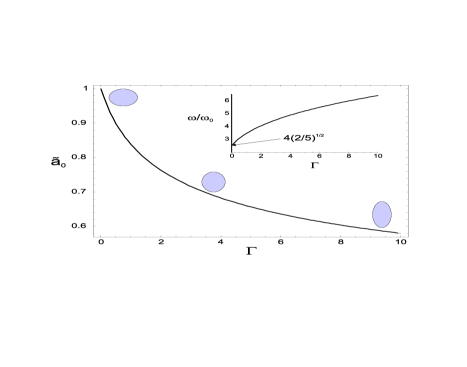
Figure 2: (color online) The droplet shape, characterized by the semiminor axis expressed in units $r_{0}$ of the spherical droplet with the same volume, is shown as a function of the magnetic field, expressed through $\Gamma=\mu H_{a}^{2}r_{0}/(2\sigma)$. In the inset, the oscillation frequency of the quadrupole mode (in units of $\omega_{0}=\sqrt{3\sigma/(2\rho r_{0})}$) is shown as a function of $\Gamma$. The limiting value for a spherical droplet is given.

A Taylor expansion of the energy around the minimum allows to find the oscillation frequency of the quadrupole mode of the droplet. We equate the second order term in the expansion with a harmonic oscillation around the optimal shape,

$$\rho V\omega^{2} =2\pi\sigma\left.\frac{\partial^{2}\tilde{E}}{\partial\tilde{a}^{2}}\right|_{\tilde{a}_{0}}$$

$$\Rightarrow\omega=\sqrt{\frac{3\sigma}{2\rho r_{0}^{3}}\left.\frac{\partial^{2}\tilde{E}}{\partial\tilde{a}^{2}}\right|_{\tilde{a}_{0}}}.$$ (15)

Here $\rho$ is the density of the Meissner liquid. The dependence of the frequency on the magnetic field in reduced units, $\Gamma$, is shown in the inset of Fig. 2. The frequency is expressed in units $\omega_{0}=\sqrt{3\sigma/(2\rho r_{0})}.$ In the limit of spherical droplets ($H_{a}\rightarrow 0$) the frequency converges to $\omega/\omega_{0}=4\sqrt{2/5}$. For a $r_{0}=$1 mm droplet with $\sigma=10^{-3}$ J/m² and $\rho=10^{3}$ kg/m³, the unit $\omega_{0}$ corresponds to a frequency of 39 Hz. Increasing the magnetic field deforms the bubble, and also stiffens the oscillation frequency.

III Surface waves on a Meissner fluid

The quadrupole oscillation mode of the droplet is one particular realization of surface waves. In this section, we investigate how the surface waves on an infinitely deep Meissner fluid are influenced by an applied magnetic field parallel to the surface and parallel to the propagation direction of the wave (a field normal to the propagation direction of the wave would be parallel to the wave fronts and would not induce magnetic charges on the surface - thus it would not alter the wave dispersion).

Figure 3: (color online) The magnetization of a Meissner fluid with a surface wave is shown in panel (a); the applied field is parallel to the surface and to the wave propagation direction. The magnetization induces surface charges on the rising and descending wave slopes, as indicated. The shading (from dark blue - low to light green - high) indicates the concentration of magnetic charge. In panel (b) and (c), the demagnetization field and the total magnetic flux are shown, respectively.

Here, we consider small-amplitude waves. The surface of the liquid is characterized by $\zeta(x)=\alpha\sin(kx)$ where the flat surface corresponds to the $xy$-plane (at $z=0$), $\alpha$ is the wave amplitude, and $k=2\pi/\lambda$ is the wave number. The angle between the tangent to the surface and the horizontal plane is

$$\theta(x)=\arctan[\zeta^{\prime}(x)]=\alpha k\cos(kx)+\mathcal{O}(\alpha^{3}).$$ (16)

III.1 Demagnetization field

When the surface of the fluid is flat and the applied field $\mathbf{H}_{a}$ is parallel to the surface, the magnetization exactly cancels $\mathbf{H}_{a}=H_{a}\mathbf{e}_{x}$ to achieve the Meissner state. However, when a wave is present, the magnetization will induce surface magnetic charge on the rising and descending slopes of the wave, as illustrated in panel (a) of Fig. (3). The shading of the liquid in this figure also illustrates the concentration of this magnetic charge $\mathbf{\nabla\cdot M},$ strongest at the slopes of the wave. As in a regular magnetized object, this gives rize to a demagnetization field $\mathbf{H}_{d}$, calculated below and shown in panel (b) of Fig. (3). The resulting total flux is shown in panel (c) of that Fig. (3), and, as calculated below, follows the contour of the surface wave.

To find the magnetic field $\mathbf{H}(x,z)$ in this case, we decompose this field in a component $H_{//}$ tangential to the surface and a component $H_{\bot}$ normal to the surface. For a small-amplitude wave, $H_{\bot}$ will be of order $\alpha$ and $H_{//}\approx|H_{a}|$ up to second order in $\alpha$. The demagnetization field $\mathbf{H}_{d}=\mathbf{H}-H_{a}\mathbf{e}_{x}$ at the surface of the wave can then be written as

$$\mathbf{H}_{d}\left[x,\zeta(x)\right]$$

$$=\left\{H_{//}\cos\left[\theta(x)\right]-H_{\bot}(x)\sin\left[\theta(x)\right]-H_{a}\right\}\mathbf{e}_{x}$$

$$+\left\{H_{//}\sin[\theta(x)]+H_{\bot}(x)\cos[\theta(x)]\right\}\mathbf{e}_{z},$$ (17)

or, expanding with respect to $\alpha$,

$$\mathbf{H}_{d}\left[x,\zeta(x)\right]$$

$$=\left[-H_{a}\frac{1}{2}\alpha^{2}k^{2}\cos^{2}(kx)-H_{\bot}(x)\alpha k\cos(kx)\right]\mathbf{e}_{x}$$

$$+\left[H_{a}\alpha k\cos(kx)+H_{\bot}(x)\right]\mathbf{e}_{z}+\mathcal{O}(\alpha^{3}).$$ (18)

For the calculation of the energy associated with the magnetization, we need to find the demagnetization field inside the fluid. As a trial solution, we use

$$\mathbf{H}_{d}^{in}(x,z)=\mathbf{h}(x)e^{k(z-\zeta(x))}.$$ (19)

That is, we assume an exponential decay into the fluid with the wave length of the surface wave as a characteristic scale. In the direction of propagation of the wave, we need to find $\mathbf{h}(x)=h_{x}(x)\mathbf{e}_{x}+h_{z}(x)\mathbf{e}_{z}.$ The ansatz (19) allows to satisfy $\nabla\times\mathbf{H}_{d}^{in}=0,$ which reduces to

$$\frac{\partial h_{z}(x)}{\partial x}-h_{z}(x)\alpha k^{2}\cos(kx)=kh_{x}(x),$$ (20)

with boundary conditions $\mathbf{h}(x)=\mathbf{H}_{d}\left[x,\zeta(x)\right]$ and $\mathbf{h}(x)=\mathbf{h}(x+\lambda)$. This can be solved straightforwardly, yielding

$$\mathbf{H}_{d}\left[x,z<\zeta(x)\right] =H_{a}\frac{\alpha^{2}k^{2}}{2}\cos^{2}(kx)$$

$$\times\exp\{k\left[z-\alpha\sin(kx)\right]\}\mathbf{e}_{x}.$$ (21)

for the demagnetization field inside the liquid.

III.2 Magnetic energy

Consider a surface of fluid of length $L_{y}$ in the $y$-direction and $L_{x}=p\lambda$ ($p\in\mathbb{N})$ in the $x$-direction. The energy difference $E_{mag}$ between the unmagnetized ($\mathbf{H}_{a}=0$) and the magnetized case can be written as

$$E_{mag}=\frac{\mu}{2}\underset{z<\zeta(x)}{\int}\mathbf{H}_{a}\cdot\mathbf{H}_{d}d^{3}\mathbf{r}+\frac{\mu}{2}\int\mathbf{H}_{a}^{2}d^{3}\mathbf{r}.$$ (22)

The second term represents the energy of swichting on the applied magnetic field, and does not depend on the presence of a surface wave. The first term evaluates to

$$E_{mag} =\frac{\mu H_{a}^{2}}{2}\frac{\alpha^{2}k}{2}L_{y}\int_{0}^{L_{x}}dx\cos^{2}(kx)$$

$$=\frac{1}{4}\frac{\mu H_{a}^{2}}{2}k\text{ }L_{x}L_{y}\ \alpha^{2}.$$

Thus, the magnetic energy per unit surface required to establish the Meissner state when there is a surface wave with wave number $k$ and amplitude $\alpha$ is (to order $\alpha^{3}$) given by

$$E_{M}=\frac{\mu H_{a}^{2}}{8}k\alpha^{2}.$$ (23)

III.3 Wave dispersion

To find the dispersion relation of a surface wave on an infinitely deep Meissner fluid, we follow the Hamiltonian procedure outlined in Ref. KlemensAJP52 . The kinetic energy per unit surface, associated with the surface wave is

$$E_{K}=\frac{1}{4}\frac{\rho}{k}\dot{\alpha}^{2}.$$ (24)

When the flat surface is deformed, restoring forces tend to pull it flat again. These restoring forces can be related to the surface tension energy, per unit surface:

$$E_{S} =\frac{1}{L_{x}}\overset{L_{x}}{\underset{0}{\int}}\frac{1}{2}\sigma\left(\frac{\partial\zeta(x)}{\partial x}\right)^{2}dx$$

$$=\frac{1}{4}\sigma k^{2}\alpha^{2},$$ (25)

and to the gravitational energy, per unit surface:

$$E_{G}=\frac{1}{4}\rho g\alpha^{2}.$$ (26)

In a Meissner liquid, subjected to a magnetic field parallel to the surface wave propagation direction, also the magnetic energy (23) gives rise to a restoring force. The (classical) Hamiltonian associated with the surface wave of amplitude $\alpha$ is then given by the sum of (24),(25),(26) and (23) :

$$H=\frac{1}{4}\frac{\rho}{k}\dot{\alpha}^{2}+\left(\frac{1}{4}\sigma k^{2}+\frac{1}{4}\rho g+\frac{1}{4}\frac{\mu H_{a}^{2}}{2}k\right)\alpha^{2}.$$ (27)

This expression is valid for small-amplitude oscillations, and leads to a dispersion relation

$$\omega(k)=\sqrt{\frac{\sigma k^{3}}{\rho}+\frac{\mu H_{a}^{2}}{2}\frac{k^{2}}{\rho}+gk}.$$ (28)

The effect of the magnetic field dominates when $\mu H_{a}>>\sqrt{\mu\rho g/k}$ and $\mu H_{a}>>\sqrt{\mu\sigma k}.$ Taking again $\sigma=10^{-3}$ J/m² and $\rho=10^{3}$ kg/m³, and a magnetic field of $\mu H_{a}=100$ G, we find that the Meissner contribution to the dispersion dominates for $10^{2}$ m${}^{-1}\lesssim k\lesssim 10^{5}$ m${}^{-1}.$ The experimental setup of Ref. TaoPRB68 would allow to probe this range of wave lengths. Surface waves can be detected by reflecting a laser beam off the surface of the Meissner fluid and noting the displacement of the laser spot as a function of time and space.

IV Conclusion

Fluids with remarkable magnetic response properties, such as ferrofluids, have sparked a lot of interest. Here, we investigate how a fluid superconductor, a Meissner fluid, would react to an applied magnetic field. Even though such Meissner fluids are not yet accessible, candidate realizations from theory BabaevNAT431 and recent experiments TaoPRL83 can be found.

When such a fluid superconducting material is placed in an applied magnetic field, it will flow to adapt its shape and minimize the energy required to expell the magnetic flux. In this contribution, we focused on a single droplet of Meissner fluid and derived the deformation of such a droplet due to an applied magnetic field as well as the associated quadrupole oscillation frequency. Inversely, imposing a hydrodynamic flow, for example by generating a surface wave, will alter the energetics and thus the dispersion of the wave. We calculated how the dispersion of the surface wave is changed due to the presence of a magnetic field, applied parallel to the surface and to the propagation direction of the wave. The change in the dispersion is predicted to be relevant for the wave length range thought to be achievable in a setup such as TaoPRL83 .

- (1) J. E. Jaffe and N. W. Ashcroft, Phys. Rev. B 23, 6176 (1981).
- (2) E. Babaev, A. Sudbø, and N. W. Ashcroft, Nature 431, 666 (2004).
- (3) R. Tao, X. Zhang, X. Tang, and P. W. Anderson, Phys. Rev. Lett. 83, 5575 (1999).
- (4) R. Tao, X. Xu, and E. Amr, Phys. Rev. B 68, 144505 (2003).
- (5) M. Liu, Journ. Low. Temp. Phys. 126, 911 (2002).
- (6) M. Liu, Phys. Rev. Lett. 70, 3580 - 3583 (1993).
- (7) C. Birch, Eur. J. Phys. 6, 180 (1985).
- (8) J. A. Cape, J. M. Zimmerman, Phys. Rev. 153, 416 (1967).
- (9) P. Moon and D.E. Spencer, Field Theory Handbook (Springer-Verlag, 1971), p. 28-36.
- (10) P.G. Klemens, Am. J. Phys. 52, 451 (1984).