A Homogeneous Sample of Sub-DLAs IV:                                     Global Metallicity Evolution

Abstract

An accurate method to measure the abundance of high-redshift galaxies consists in the observation of absorbers along the line of sight toward a background quasar. Here, we present abundance measurements of 13 $z\geq 3$ sub-Damped Lyman-$\alpha$ Systems (quasar absorbers with H i column density $19$ $<$ log N(HI) $<$ 20.3 cm^-2) based on the high resolution observations with VLT UVES spectrograph. These observations more than double the metallicity information for sub-DLAs previously available at $z>3$. This new data, combined with other sub-DLA measurements from the literature, confirm the stronger metallicity redshift evolution than for the classical Damped Lyman-$\alpha$ absorbers. Besides, these observations are used to compute for the first time the fraction of gas ionised from photo-ionisation modelling in a sample of sub-DLAs. Based on these results, we calculate that sub-DLAs contribute no more than 6% of the expected amount of metals at z$\sim$ 2.5. We therefore conclude that even if sub-DLAs are found to be more metal-rich than classical DLAs, they are insufficient to close the so-called “missing metals problem”.

1 Introduction

Damped Lyman-$\alpha$ systems (hereafter DLAs) seen in absorption in the spectra of background quasars are selected over all redshifts independent of their intrinsic luminosity. They have hydrogen column densities, log $N({\rm HI})\geq 20.3$. DLAs are also contributors to the neutral gas, $\Omega_{\rm HI}$, in the Universe at high redshifts and it is from this gas reservoir that the stars visible today formed (Wolfe et al. 1995). Furthermore, DLAs offer a direct and accurate probe of elemental abundances over $>90\%$ of the age of the Universe.

Recently, much attention has been drawn to the sub-Damped Lyman-$\alpha$ Systems. These systems have H i column density $19$ $<$ log N(HI) $<$ 20.3 cm^-2 and were first coined by Péroux et al. (2003a). In a series of paper, our group has analysed a unique homogeneous sample of sub-DLAs all observed at the same resolution with the same instrument on the Very Large Telescope (VLT). The first two papers are based on the ESO/UVES archives (Paper I: Dessauges-Zavadsky et al. 2003; Paper II: Péroux et al. 2003b) while more recent studies are from our own observational programmes (Paper III: Péroux et al. 2005; Paper IV: this paper) leading to a new sample of high-redshift sub-DLAs observed under the same conditions. These works as well as other recent studies are suggesting that high metallicities can be found more easily in sub-DLAs than in classic DLAs, especially a low-redshift (e.g., Pettini et al. 2000; Jenkins et al. 2005; Péroux et al. 2006a; Prochaska et al. 2006; Péroux et al. 2006b). In the present paper, we study a new sample of high-redshift sub-DLAs to better constrain their metallicities at $z>3$. In addition, our data are used in combination with others from the literature to compute the fraction of ionised gas in a sample of sub-DLAs and reliably compute the contribution of sub-DLAs to the global metallicity.

The paper is structure as follows. In the second section, we present the methodology and results of the determination of the chemical content of these high-redshift sub-DLAs. In the third section, the total abundances including results from detailed photo-ionisation models are given and the redshift evolution of the metallicity is presented. Finally, the last section describes the contribution of sub-DLAs to the global metallicity in the context of the so-called missing metals problem.

2 A Sample of 13 $z\geq 3$ Sub-DLAs

Table 1 summarises the absorption redshift and $N_{\rm HI}$ column densities for each of the 13 $z\geq 3$ sub-DLAs which constitute the sample under study. The data acquisition and reduction are described in Péroux et al. (2005). In the case of PSS J0133$+$0400, our own data have been supplemented by a 3000 sec exposure with setting 860 (ESO 74.A-0306, P.I.: Valentina D’Odorico) and a 5200 sec exposure with setting 540 (ESO 73.A-0071, P.I.: Cédric Ledoux).

In this section, details on each of the studied sub-DLAs are provided. The metals associated with the Lyman lines were searched over the spectral coverage available. More than the 40 transitions most frequently detected in high column density quasar absorbers have been systematically looked for. The metal column densities are then determined by fitting Voigt profiles to the absorption lines. The fits were performed using the $\chi^{2}$ minimisation routine fitlyman in MIDAS (Fontana & Ballester 1995).

Table 1: The sample of 13 high-redshift sub-DLAs for which abundance studies have been undertaken.

Quasar	$z_{\rm em}$	$z_{\rm abs}$	$\log N_{\rm HI}$
PSS J0118$+$0320	4.230	4.128	20.02$\pm$0.15
PSS J0121$+$0347	4.127	2.976	19.53$\pm$0.10
SDSS J0124$+$0044	3.840	2.988	19.18$\pm$0.10
…	…	3.078	20.21$\pm$0.10
PSS J0133$+$0400	4.154	3.139	19.01$\pm$0.10
…	…	3.995	19.94$\pm$0.15
…	…	3.999	19.16$\pm$0.15
…	…	4.021	19.09$\pm$0.15
BRI J0137$-$4224	3.970	3.101	19.81$\pm$0.10
…	…	3.665	19.11$\pm$0.10
BR J2215$-$1611	3.990	3.656	19.01$\pm$0.15
…	…	3.662	20.05$\pm$0.15
BR J2216$-$6714	4.469	3.368	19.80$\pm$0.10

1. PSS J0118$+$0320 ($z_{\rm em}$=4.230, $z_{\rm abs}$=4.128, $\log N_{\rm HI}$=20.02$\pm$0.15):

   This system is at the high end of the sub-DLA definition with $\log N_{\rm HI}$=20.02$\pm$0.15. Many metal lines are detected at $z_{\rm abs}$=4.128, some of which are clearly saturated. The fit is done using simultaneously Fe ii $\lambda$ 1608, Fe ii $\lambda$ 1144, Si ii $\lambda$ 1526, Si ii $\lambda$ 1304, S ii $\lambda$ 1259 and S ii $\lambda$ 1253 to derive the redshifts and $b$ parameters of the 5 components. The fit is shown in Figure 1 and the matching parameters are presented in Table 2. In this and the following tables velocities and $b$ are in km s^-1 and N’s are in cm^-2. Lower limits for $\rm C~{}{\sc ii}$ and $\rm O~{}{\sc i}$ are derived from the saturated lines. The Zn ii $\lambda$ 2026 line is covered by our spectrum but is situated in a region too noisy to allow to derive any meaningful upper limit.

   Both $\rm Si~{}{\sc iv}$ and $\rm C~{}{\sc iv}$ high-ionisation doublets are detected. The redshifts and $b$ of the 9 components are derived from a simultaneous fit of C iv $\lambda$ 1548, C iv $\lambda$ 1550 and Si iv $\lambda$ 1393 (Si iv $\lambda$ 1402 is affected by telluric lines). The resulting fit is overplotted on Si iv $\lambda$ 1402 for consistency check. The fit is shown in Figure 2 and the matching parameters are presented in Table 3.

   Table 2: Parameters fit to the low-ionisation transitions of the $z_{\rm abs}$=4.128 $\log N_{\rm HI}$=20.02$\pm$0.15 sub-DLA towards PSS J0118$+$0320.

   z	$b$	log N($\rm Fe~{}{\sc ii}$)	log N($\rm Si~{}{\sc ii}$)	log N($\rm C~{}{\sc ii}$)	log N($\rm O~{}{\sc i}$)	log N($\rm S~{}{\sc ii}$)
   4.127836	4.61$\pm$0.14	13.21$\pm$0.11	13.60$\pm$0.02	$>$15.35	$>$13.95	13.41$\pm$0.11
   4.128319	30.06$\pm$0.21	13.57$\pm$0.12	14.14$\pm$0.02	$>$14.58	$>$15.15	13.94$\pm$0.11
   4.128678	3.11$\pm$0.14	13.71$\pm$0.11	14.69$\pm$0.04	$>$17.28	$>$16.37	13.75$\pm$0.11
   4.129264	3.30$\pm$0.18	13.43$\pm$0.12	13.42$\pm$0.02	$>$15.64	$>$14.02	13.02$\pm$0.13
   4.129627	6.87$\pm$0.25	13.12$\pm$0.11	12.73$\pm$0.01	$>$12.60	$>$12.00	11.89$\pm$0.12

   

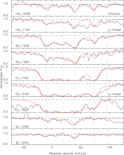
   Figure 1: Fit to the low-ionisation transitions of the $z_{\rm abs}$=4.128 $\log N_{\rm HI}$=20.02$\pm$0.15 sub-DLA towards PSS J0118$+$0320 (see Table 2). In this and the following figures, the zero velocity corresponds to the absorption redshift listed in Table 1, the vertical dashed lines correspond to the fitted components and the mention ’Ly forest’ means that the metal line falls in the Lyman-$\alpha$ forest of the quasar spectrum while ’Tellurics’ indicates a region contaminated by telluric lines.

   Table 3: Parameters fit to the high-ionisation transitions of the $z_{\rm abs}$=4.128 $\log N_{\rm HI}$=20.02$\pm$0.15 sub-DLA towards PSS J0118$+$0320.

   z	$b$	log N($\rm C~{}{\sc iv}$)	log N($\rm Si~{}{\sc iv}$)
   4.126680	29.70$\pm$0.26	13.49$\pm$0.12	13.17$\pm$0.12
   4.127345	9.90$\pm$0.13	13.19$\pm$0.12	12.47$\pm$0.12
   4.128024	22.20$\pm$0.31	13.30$\pm$0.11	12.71$\pm$0.22
   4.128656	11.10$\pm$0.12	13.30$\pm$0.33	12.56$\pm$0.12
   4.129083	21.60$\pm$0.23	13.59$\pm$0.11	13.04$\pm$0.11
   4.129787	3.20$\pm$0.02	13.04$\pm$0.12	12.30$\pm$0.12
   4.130161	8.70$\pm$0.04	13.50$\pm$0.11	12.97$\pm$0.12
   4.130446	2.60$\pm$0.01	13.08$\pm$0.12	12.65$\pm$0.12
   4.130711	9.00$\pm$0.08	13.31$\pm$0.11	12.84$\pm$0.12

   

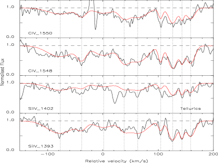
   Figure 2: Fit to the high-ionisation transitions of the $z_{\rm abs}$=4.128 $\log N_{\rm HI}$= 20.02$\pm$0.15 sub-DLA towards PSS J0118$+$0320 (see Table 3).

2. PSS J0121$+$0347 ($z_{\rm em}$=4.127, $z_{\rm abs}$=2.976, $\log N_{\rm HI}$=19.53$\pm$0.10):

   The low-ionisation transitions in this system are well fitted with one component, the redshift and $b$ of which are fixed by a simultaneous fit of Si ii $\lambda$ 1260, O i $\lambda$ 1302, C ii $\lambda$ 1334, Fe ii $\lambda$ 1608 and Al ii $\lambda$ 1670. The first four lines are situated in the Lyman-$\alpha$ forest. This explains the likely blending which affects them. Therefore, measurements from $\rm Si~{}{\sc iii}$, $\rm O~{}{\sc i}$ and $\rm C~{}{\sc ii}$ are considered as upper limits. The fit is shown in Figure 3 and the matching parameters are presented in Table 4. Al iii $\lambda$ 1854 and Al iii $\lambda$ 1862 are covered but not detected. An upper limit is derived for the Al abundance: log N($\rm Al~{}{\sc iii}$)$<$11.77 at 4$\sigma$.

   Interestingly, in this system the high-ionisation transitions is partially fitted with the same velocity component than for the low-ionisation transitions. The $\rm C~{}{\sc iv}$ and $\rm Si~{}{\sc iv}$ doublets are fitted simultaneously. $\rm C~{}{\sc iv}$ is heavily blended and therefore leads to an upper limit, while $\rm Si~{}{\sc iv}$ is nicely fitted from the Si iv $\lambda$ 1393 line. The fit is shown in Figure 4 and the matching parameters are presented in Table 5.

   Table 4: Parameters fit to the low-ionisation transitions of the $z_{\rm abs}$=2.976 $\log N_{\rm HI}$=19.53$\pm$0.10 sub-DLA towards PSS J0121$+$0347.

   z	$b$	log N($\rm Fe~{}{\sc ii}$)	log N($\rm Si~{}{\sc ii}$)	log N($\rm C~{}{\sc ii}$)	log N($\rm O~{}{\sc i}$)	log N($\rm Al~{}{\sc iii}$)
   2.976613	9.90$\pm$0.94	13.18$\pm$0.30	$<$13.15	$<$13.72	$<$13.98	11.93$\pm$0.32

   

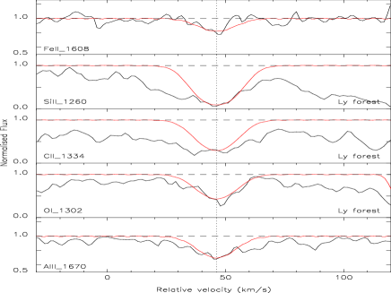
   Figure 3: Fit to the low-ionisation transitions of the $z_{\rm abs}$=2.976 $\log N_{\rm HI}$=19.53$\pm$0.10 sub-DLA towards PSS J0121$+$0347 (see Table 4).

   Table 5: Parameters fit to the high-ionisation transitions of the $z_{\rm abs}$=2.976 $\log N_{\rm HI}$=19.53$\pm$0.10 sub-DLA towards PSS J0121$+$0347.

   z	$b$	log N($\rm C~{}{\sc iv}$)	log N($\rm Si~{}{\sc iv}$)
   2.975965	11.90$\pm$0.08	$<$13.50	13.10$\pm$0.10
   2.976579	16.90$\pm$0.08	$<$13.47	12.95$\pm$0.10

   

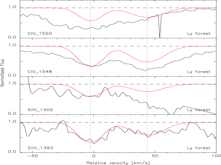
   Figure 4: Fit to the high-ionisation transitions of the $z_{\rm abs}$=2.976 $\log N_{\rm HI}$=19.53$\pm$0.10 sub-DLA towards PSS J0121$+$0347 (see Table 5).

3. SDSS J0124$+$0044 ($z_{\rm em}$=3.840, $z_{\rm abs}$=2.988, $\log N_{\rm HI}$=19.18$\pm$0.10):

   This system has low-ionisation lines which cover a rather large velocity range and the profiles are well characterised by two separate clumps at $\sim-$100 km s^-1 and $\sim+$30 km s^-1. A simultaneous fit to Al ii $\lambda$ 1670 and Si ii $\lambda$ 1526 is used to derive the redshifts and $b$ of the 4 components in the low-ionisation transitions of the sub-DLA at $z_{\rm abs}$=2.988 towards SDSS J0124$+$0400. These results are checked for consistency with many other $\rm Si~{}{\sc iii}$ lines (Si ii $\lambda$ 1193, Si ii $\lambda$ 1190, Si ii $\lambda$ 1260 and Si ii $\lambda$ 1526 – Si ii $\lambda$ 1808 is not covered by our data). The same redshifts and $b$ are used to derive the column density of C ii $\lambda$ 1334 and upper limits from S ii $\lambda$ 1253, S ii $\lambda$ 1259 and Fe iii $\lambda$ 1122 which are all probably blended by lines from the Lyman-$\alpha$ forest. Similarly, an upper limit is derived for $\rm Fe~{}{\sc ii}$ using the many lines falling in the forest (Fe ii $\lambda$ 1063, Fe ii $\lambda$ 1096, Fe ii $\lambda$ 1121, Fe ii $\lambda$ 1125, Fe ii $\lambda$ 1143 and Fe ii $\lambda$ 1144) as well as Fe ii $\lambda$ 1608. The fit is shown in Figure 5 and the matching parameters are presented in Table 6. The two $\rm Al~{}{\sc iii}$ lines are not covered by our spectrum for this system.

   The $\rm C~{}{\sc iv}$ doublet is nicely fitted with 7 components, the two first being the strongest ones. The $\rm Si~{}{\sc iv}$ doublet is blended but is nevertheless fitted using the same components in order to derive an upper limit on the abundance. Note however, that there is no physical reason suggesting that $\rm C~{}{\sc iv}$ and $\rm Si~{}{\sc iv}$ should come from the same region, i.e. should have the same velocity profile. It is just an empirical fact that in DLAs, this is often the case. The fit is shown in Figure 6 and the matching parameters are presented in Table 7.

   Table 6: Parameters fit to the low-ionisation transitions of the $z_{\rm abs}$=2.988 $\log N_{\rm HI}$=19.18$\pm$0.10 sub-DLA towards SDSS J0124$+$0044.

   z	$b$	log N($\rm Fe~{}{\sc ii}$)	log N($\rm Si~{}{\sc ii}$)	log N($\rm C~{}{\sc ii}$)	log N($\rm S~{}{\sc ii}$)	log N($\rm Al~{}{\sc ii}$)	log N($\rm Fe~{}{\sc iii}$)
   2.986404	2.90$\pm$0.01	$<$12.62	13.41$\pm$0.13	$<$15.67	$<$13.48	11.68$\pm$0.16	$<$13.39
   2.986680	12.50$\pm$0.61	$<$13.20	13.98$\pm$0.11	$<$14.62	$<$13.59	12.58$\pm$0.12	$<$13.59
   2.988448	12.80$\pm$0.03	$<$13.00	12.71$\pm$0.16	$<$13.53	$<$13.88	11.82$\pm$0.13	$<$13.51
   2.988998	8.50$\pm$0.20	$<$12.72	12.78$\pm$0.16	$<$14.07	$<$13.63	11.93$\pm$0.14	$<$13.44

   

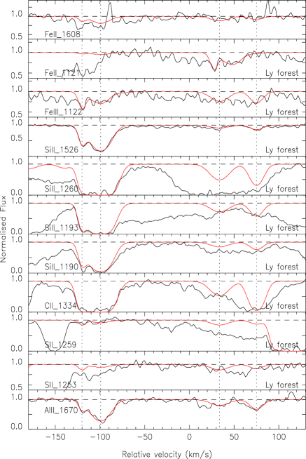
   Figure 5: Fit to the low-ionisation transitions of the $z_{\rm abs}$=2.988 $\log N_{\rm HI}$=19.18$\pm$0.10 sub-DLA towards SDSS J0124$+$0044 (see Table 6).

   Table 7: Parameters fit to the high-ionisation transitions of the $z_{\rm abs}$=2.988 $\log N_{\rm HI}$=19.18$\pm$0.10 sub-DLA towards SDSS J0124$+$0044.

   z	$b$	log N($\rm C~{}{\sc iv}$)	log N($\rm Si~{}{\sc iv}$)
   2.986426	9.40$\pm$0.01	13.60$\pm$0.02	$<$13.00
   2.986677	14.70$\pm$0.61	14.19$\pm$0.18	$<$13.59
   2.987084	10.70$\pm$0.03	13.44$\pm$0.02	$<$13.34
   2.987509	15.60$\pm$0.02	13.31$\pm$0.08	$<$13.41
   2.988232	11.94$\pm$0.10	13.10$\pm$1.04	$<$13.34
   2.988896	17.70$\pm$0.05	13.01$\pm$0.07	$<$13.47
   2.989483	5.70$\pm$0.05	12.33$\pm$1.41	$<$12.97

   

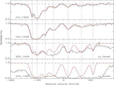
   Figure 6: fit to the high-ionisation transitions of the $z_{\rm abs}$=2.988 $\log N_{\rm HI}$=19.18$\pm$0.10 sub-DLA towards SDSS J0124$+$0044 (Table 7).

4. SDSS J0124$+$0044 ($z_{\rm em}$=3.840, $z_{\rm abs}$=3.078, $\log N_{\rm HI}$=20.21$\pm$0.10):

   This system has fairly high H i column density of $\log N_{\rm HI}$=20.21$\pm$0.10. The Si ii $\lambda$ 1304 and Si ii $\lambda$ 1526 profiles of the sub-DLA at $z_{\rm abs}$=3.078 are well fitted by two components. The results of this simultaneous fit is applied on the blended Si ii $\lambda$ 1190, Si ii $\lambda$ 1193 and Si ii $\lambda$ 1260 for consistency check. The same redshifts and $b$ are used to put limits on O i $\lambda$ 1302, C ii $\lambda$ 1334 and Fe ii $\lambda$ 1096, Fe ii $\lambda$ 1125, Fe ii $\lambda$ 1144 and Fe ii $\lambda$ 1608. $\rm O~{}{\sc i}$ and $\rm C~{}{\sc ii}$ are clearly saturated and lead to lower limits. A column density for Fe ii $\lambda$ is constrained from a combination of the red wing of Fe ii $\lambda$ 1608 and the blue wing of Fe ii $\lambda$ 1096 and is consistent with all the other Fe ii $\lambda$ lines available. The fit is shown in Figure 7 and the matching parameters are presented in Table 8.

   The $\rm Si~{}{\sc iv}$ doublet associated with this system is totally blended in the forest but the $\rm C~{}{\sc iv}$ seems to be detected as an extremely broad b$>$100 km s${-1}$ single component line. The strength of the two $\rm C~{}{\sc iv}$ lines of the doublet are consistent with their respective oscillator strengths, but they do not display the characteristic complex profiles of sub-DLA/DLAs. Therefore, care should be taken in interpreting these features as $\rm C~{}{\sc iv}$. The column density we derive is N($\rm C~{}{\sc iv}$)=13.92$\pm$0.11 but this system might as well be a large $N_{\rm HI}$ system with no $\rm C~{}{\sc iv}$ detected. This is illustrated in Figure 8.

   Table 8: Parameters fit to the low-ionisation transitions of the $z_{\rm abs}$=3.078 $\log N_{\rm HI}$=20.21$\pm$0.10 sub-DLA towards SDSS J0124$+$0044.

   z	$b$	log N($\rm Fe~{}{\sc ii}$)	log N($\rm Si~{}{\sc ii}$)	log N($\rm C~{}{\sc ii}$)	log N($\rm O~{}{\sc i}$)
   3.077625	6.20$\pm$3.20	$<$13.95	13.75$\pm$0.20	$>$14.93	$>$15.00
   3.077758	2.10$\pm$0.40	$<$13.65	15.11$\pm$0.40	$>$15.15	$>$14.60

   

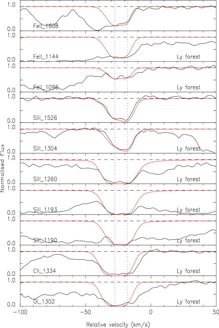
   Figure 7: Fit to the low-ionisation transitions of the $z_{\rm abs}$=3.078 $\log N_{\rm HI}$=20.21$\pm$0.10 sub-DLA towards SDSS J0124$+$0044 (see Table 8).

   

   Figure 8: High-ionisation ions of the absorber detected towards SDSS J0124$+$0044 with $\log N_{\rm HI}$=20.21$\pm$0.10 at $z_{\rm abs}$=3.078.

5. PSS J0133$+$0400 ($z_{\rm em}$=4.154, $z_{\rm abs}$=3.139, $\log N_{\rm HI}$=19.01$\pm$0.10):

   This sub-DLA has a low $N_{\rm HI}$ column density with $\log N_{\rm HI}$=19.01$\pm$0.10 at $z_{\rm abs}$=3.139. Unfortunately, many of the expected strong metal lines for this system fall in spectral gaps (i.e. Fe ii $\lambda$ 1608, C iv $\lambda$ 1548, C iv $\lambda$ 1550) or are blended with H i lines from the Lyman-$\alpha$ forest (i.e. the other Fe ii $\lambda$ lines). The two component fit was performed on Si ii $\lambda$ 1260 with a consistency check on Si ii $\lambda$ 1808 to derive an upper limit on the total SiII column density. Attempts to increase the number of components does not improve the $\chi^{2}$ of the fit in this case. The same redshifts and $b$ were applied on the blended C ii $\lambda$ 1334 to derive an upper limit on the C abundance. The fit is shown in Figure 9 and the matching parameters are presented in Table 9. Al iii $\lambda$ 1854 is strongly blended, but Al iii $\lambda$ 1862 is used to derive an 4$\sigma$ upper limit: log N($\rm Al~{}{\sc iii}$)$<$11.44.

   The position of the high-ionisation transitions are unfortunate in this system too. The Si iv $\lambda$ 1402 falls in a DLA along the same sight-of-line while the Si iv $\lambda$ 1393 is completely blended with H i lines from the Lyman-$\alpha$ forest. The $\rm C~{}{\sc iv}$ doublet is situated in one of the spectral gap of our data.

   Table 9: Parameters fit to the low-ionisation transitions of the $z_{\rm abs}$=3.139 $\log N_{\rm HI}$=19.01$\pm$0.10 sub-DLA towards PSS J0133$+$0400.

   z	$b$	log N($\rm Si~{}{\sc ii}$)	log N($\rm C~{}{\sc ii}$)
   3.138360	31.60$\pm$0.20	$<$12.87	$<$13.25
   3.139605	7.40$\pm$0.10	$<$12.81	$<$13.72

   

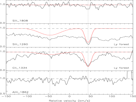
   Figure 9: Fit to the low-ionisation transitions of the $z_{\rm abs}$=3.139 $\log N_{\rm HI}$=19.01$\pm$0.10 sub-DLA towards PSS J0133$+$0400 (see Table 9). The fit of C ii $\lambda$ 1334 is used to derive an upper limit on the $\rm C~{}{\sc ii}$ column density.

6. PSS J0133$+$0400 ($z_{\rm em}$=4.154, $z_{\rm abs}$=3.995, $\log N_{\rm HI}$=19.94$\pm$0.15):

   This system has a fairly high $N_{\rm HI}$ with $\log N_{\rm HI}$=19.94$\pm$0.15 at $z_{\rm abs}$=3.995. The redshifts and $b$ of the 5 components were derived from partially blended lines of Si ii $\lambda$ 1260 (telluric contamination) for two bluest components and Si ii $\lambda$ 1190 (Lyman-$\alpha$ forest contamination) for the three remaining components. The resulting fit was checked upon other $\rm Si~{}{\sc iii}$ lines (Si ii $\lambda$ 1193, Si ii $\lambda$ 1260 and Si ii $\lambda$ 1808). As a result, we can obtain a good value of the total N($\rm Si~{}{\sc ii}$). Most of the Fe ii $\lambda$ lines in this system are blended with Lyman-$\alpha$ forest features (Fe ii $\lambda$ 1063, Fe ii $\lambda$ 1096, Fe ii $\lambda$ 1121 and Fe ii $\lambda$ 1125) or fall in a zero flux gap (Fe ii $\lambda$ 1143 and Fe ii $\lambda$ 1144) due to DLAs along the same line-of-sight. Only the Fe ii $\lambda$ 1608 line is covered by our spectrum but it is undetected. We derive an upper limit log N($\rm Fe~{}{\sc ii}$)$<$13.56 at 4$\sigma$. Other ions are not detected and allow the derivation of upper limits: log N($\rm Ni~{}{\sc ii}$)$<$12.31, log N($\rm Al~{}{\sc ii}$)$<$11.36 and log N($\rm Al~{}{\sc iii}$)$<$11.69. The fit is shown in Figure 10 and the matching parameters are presented in Table 10.

   The 5 components for the high-ionisation transitions are derived from a simultaneous fit of the lines Si iv $\lambda$ 1393 and Si iv $\lambda$ 1402. Si iv $\lambda$ 1393 provides a column density determination free from any contamination. The same redshifts and $b$ are used to fit the $\rm C~{}{\sc iv}$ doublet of the system and derive an upper limit on this blended lines. The fit is shown in Figure 11 and the matching parameters are presented in Table 11.

   Table 10: Parameters fit to the low-ionisation transitions of the $z_{\rm abs}$=3.995 $\log N_{\rm HI}$=19.94$\pm$0.15 sub-DLA towards PSS J0133$+$0400.

   z	$b$	log N($\rm Si~{}{\sc ii}$)
   3.994089	3.10$\pm$0.16	12.24$\pm$0.12
   3.994422	8.50$\pm$0.11	12.83$\pm$0.11
   3.995350	5.90$\pm$0.21	13.56$\pm$0.14
   3.995771	20.00$\pm$0.15	13.22$\pm$0.11
   3.996604	4.70$\pm$0.11	13.29$\pm$0.18

   

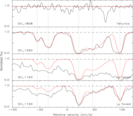
   Figure 10: Fit to the low-ionisation transitions of the $z_{\rm abs}$=3.995 $\log N_{\rm HI}$=19.94$\pm$0.15 sub-DLA towards PSS J0133$+$0400 (see Table 10).

   Table 11: Parameters fit to the high-ionisation transitions of the $z_{\rm abs}$=3.995 $\log N_{\rm HI}$=19.94$\pm$0.15 sub-DLA towards PSS J0133$+$0400.

   z	$b$	log N($\rm C~{}{\sc iv}$)	log N($\rm Si~{}{\sc iv}$)
   3.994154	8.90$\pm$ 0.01	$<$12.92	12.99$\pm$0.25
   3.994482	9.30$\pm$ 0.86	$<$12.94	12.90$\pm$0.03
   3.994817	9.30$\pm$ 0.03	$<$12.93	12.47$\pm$0.49
   3.995580	3.20$\pm$ 0.92	$<$11.95	12.24$\pm$0.42
   3.996051	15.60$\pm$ 1.33	$<$12.79	12.89$\pm$0.01

   

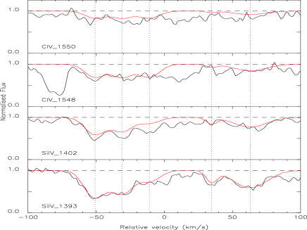
   Figure 11: Fit to the high-ionisation transitions of the $z_{\rm abs}$=3.995 $\log N_{\rm HI}$=19.94$\pm$0.15 sub-DLA towards PSS J0133$+$0400 (see Table 11).

7. PSS J0133$+$0400 ($z_{\rm em}$=4.154, $z_{\rm abs}$=3.999, $\log N_{\rm HI}$=19.16$\pm$0.15):

   This system is at the low end of the column density distribution for sub-DLAs with $\log N_{\rm HI}$=19.16$\pm$0.15 at $z_{\rm abs}$=3.999. Most $\rm Si~{}{\sc iii}$ lines are covered in this absorber but many are blended with Lyman-$\alpha$ forest contamination (i.e. Si ii $\lambda$ 1190, Si ii $\lambda$ 1193) or telluric contamination (Si ii $\lambda$ 1260, Si ii $\lambda$ 1526). Si ii $\lambda$ 1304 falls in a spectral gap. Therefore, the region around the expected position for Si ii $\lambda$ 1808 is used to derive an upper limit on the abundance of $\rm Si~{}{\sc iii}$: log N($\rm Si~{}{\sc ii}$)$<$14.12 at 4$\sigma$. Similarly, upper limits are derived for non-detection as follows: log N($\rm Al~{}{\sc ii}$)$<$11.10 from Al ii $\lambda$ 1670, log N($\rm Al~{}{\sc iii}$)$<$11.63 from Al iii $\lambda$ 1854 and log N($\rm Fe~{}{\sc ii}$)$<$13.56 from Fe ii $\lambda$ 1608.

   For the high-ionisation transitions, a fit is performed on C iv $\lambda$ 1548 and C iv $\lambda$ 1550 simultaneously. The same redshifts and $b$ are used for the Si iv $\lambda$ 1393/1402 doublet. All these lines appear broad and quite noisy and therefore lead to upper limits. The fit is shown in Figure 12 and the matching parameters are presented in Table 12.

   Table 12: Parameters fit to the high-ionisation transitions of the $z_{\rm abs}$=3.999 $\log N_{\rm HI}$=19.16$\pm$0.15 sub-DLA towards PSS J0133$+$0400.

   z	$b$	log N($\rm C~{}{\sc iv}$)	log N($\rm Si~{}{\sc iv}$)
   3.998718	20.40$\pm$0.40	$<$13.44	$<$12.55
   3.999390	34.60$\pm$0.30	$<$13.47	$<$13.15

   

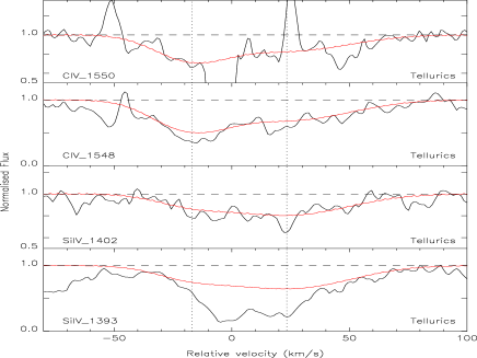
   Figure 12: Fit to the high-ionisation transitions of the $z_{\rm abs}$=3.999 $\log N_{\rm HI}$=19.16$\pm$0.15 sub-DLA towards PSS J0133$+$0400 (see Table 12).

8. PSS J0133$+$0400 ($z_{\rm em}$=4.154, $z_{\rm abs}$=4.021, $\log N_{\rm HI}$=19.09$\pm$0.15):

   This is also a system at the low end of the column density range of sub-DLAs with $\log N_{\rm HI}$=19.09$\pm$0.15 at $z_{\rm abs}$=4.021. Again, many lines for this absorber are blended in the Lyman-$\alpha$ forest. Upper limits from non-detections of Al ii $\lambda$ 1670, Si ii $\lambda$ 1808 and Fe ii $\lambda$ 1608 are derived at 4$\sigma$ level: log N($\rm Al~{}{\sc ii}$)$<$11.20, log N($\rm Si~{}{\sc ii}$)$<$14.05 and log N($\rm Fe~{}{\sc ii}$)$<$13.56.

   A kinematically simple broad absorption is detected at the position of the $\rm Si~{}{\sc iv}$ doublet. The profiles are fitted using both lines simultaneously to derive an upper limit. The $\rm C~{}{\sc iv}$ doublet however is not detected in this system. An upper limit on the abundance is derived to be log N($\rm C~{}{\sc iv}$)$<$12.31. The fit is shown in Figure 13 and the matching parameters are presented in Table 13.

   Table 13: Parameters fit to the high-ionisation transitions of the $z_{\rm abs}$=4.021 $\log N_{\rm HI}$=19.09$\pm$0.15 sub-DLA towards PSS J0133$+$0400.

   z	$b$	log N($\rm Si~{}{\sc iv}$)
   4.021325	30.3$\pm$1.00	$<$12.89

   

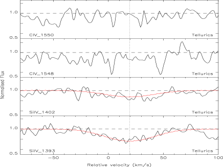
   Figure 13: Fit to the high-ionisation transitions of the $z_{\rm abs}$=4.021 $\log N_{\rm HI}$=19.09$\pm$0.15 sub-DLA towards PSS J0133$+$0400 (see Table 13).

9. BRI J0137$-$4224 ($z_{\rm em}$=3.970, $z_{\rm abs}$=3.101, $\log N_{\rm HI}$=19.81$\pm$0.10):

   The lower redshift sub-DLAs of this quasar has many metal lines falling in the Lyman-$\alpha$ forest. With a column density $\log N_{\rm HI}$=19.81$\pm$0.10 at $z_{\rm abs}$=3.101, it is situated in the mid-range of the sub-DLA definition. Nevertheless, some strong lines are undoubtfully clear from any contamination. Si ii $\lambda$ 1526 and Al ii $\lambda$ 1670 in particular are used to derive the redshifts and $b$ of the 7 components used to fit the metal-line profile. The resulting z and $b$ are used to derive the abundance of $\rm Fe~{}{\sc ii}$ from a fit to the Fe ii $\lambda$ 1608 line. The remaining Fe ii $\lambda$ lines are heavily blended with Lyman-$\alpha$ forest contamination (i.e. Fe ii $\lambda$ 1096, Fe ii $\lambda$ 1144). The fit is shown in Figure 14 and the matching parameters are presented in Table 14.

   Concerning the high-ionisation transitions, the $\rm Si~{}{\sc iv}$ doublet is falling in the Lyman-$\alpha$ forest, therefore totally blended and not useful for abundance determination. Similarly, the $\rm C~{}{\sc iv}$ doublet is blended with unidentified lines as well as with apparent emission lines which probably are the products of bad cosmic rays clipping (no telluric lines were identified in this region) and have been removed to perform the fit. The C iv $\lambda$ 1550 is fitted with 8 components and the resulting profile is made consistent with C iv $\lambda$ 1548. The fit is shown in Figure 15 and the matching parameters are presented in Table 15.

   Table 14: Parameters fit to the low-ionisation transitions of the $z_{\rm abs}$=3.101 $\log N_{\rm HI}$=19.81$\pm$0.10 sub-DLA towards BRI J0137$-$4224.

   z	$b$	log N($\rm Fe~{}{\sc ii}$)	log N($\rm Si~{}{\sc ii}$)	log N($\rm Al~{}{\sc iii}$)
   3.100382	2.90$\pm$2.64	12.65$\pm$0.39	12.92$\pm$0.33	11.73$\pm$ 0.14
   3.100559	4.90$\pm$0.11	12.95$\pm$0.01	13.40$\pm$0.20	11.88$\pm$ 0.89
   3.100821	7.40$\pm$0.91	12.70$\pm$0.01	13.64$\pm$0.29	12.20$\pm$ 0.72
   3.101004	3.30$\pm$0.12	12.80$\pm$0.12	12.73$\pm$0.22	11.40$\pm$ 0.54
   3.101679	8.00$\pm$0.77	13.20$\pm$0.01	13.45$\pm$0.25	12.33$\pm$ 0.49
   3.101915	3.20$\pm$0.22	12.70$\pm$0.01	13.25$\pm$0.10	12.06$\pm$ 0.10
   3.102078	4.10$\pm$0.40	12.10$\pm$0.01	12.27$\pm$0.20	11.48$\pm$ 0.20

   

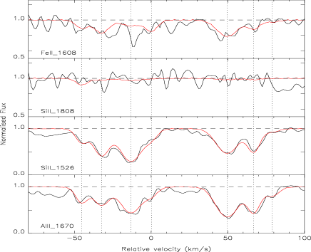
   Figure 14: Fit to the low-ionisation transitions of the $z_{\rm abs}$=3.101 $\log N_{\rm HI}$=19.81$\pm$0.10 sub-DLA towards BRI J0137$-$4224 (see Table 14).

   Table 15: Parameters fit to the high-ionisation transitions of the $z_{\rm abs}$=3.101 $\log N_{\rm HI}$=19.81$\pm$0.10 sub-DLA towards BRI J0137$-$4224.

   z	$b$	log N($\rm C~{}{\sc iv}$)
   3.100324	3.50$\pm$0.16	12.74$\pm$0.18
   3.100453	3.20$\pm$0.07	12.43$\pm$0.10
   3.100640	4.50$\pm$0.28	12.55$\pm$0.14
   3.100995	3.10$\pm$0.24	12.38$\pm$0.10
   3.101195	20.40$\pm$0.12	12.34$\pm$0.34
   3.101350	3.20$\pm$0.23	12.57$\pm$0.10
   3.101517	3.20$\pm$0.10	12.79$\pm$0.25
   3.101620	9.90$\pm$0.20	12.83$\pm$0.13

   

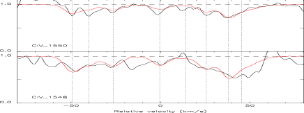
   Figure 15: Fit to the high-ionisation transitions of the $z_{\rm abs}$=3.101 $\log N_{\rm HI}$=19.81$\pm$0.10 sub-DLA towards BRI J0137$-$4224 (see Table 15).

10. BRI J0137$-$4224 ($z_{\rm em}$=3.970, $z_{\rm abs}$=3.665, $\log N_{\rm HI}$=19.11$\pm$0.10):

    This sub-DLA has a fairly low column density of $\log N_{\rm HI}$=19.11$\pm$0.10 at $z_{\rm abs}$=3.665. Nevertheless, it shows strong, kinematically simple, metal lines which are well fitted by a single component. Three lines (O i $\lambda$ 1302, Si ii $\lambda$ 1260 and C ii $\lambda$ 1334) clear from any contamination are fitted simultaneously to derive the redshift, $b$ and appropriate column densities. The resulting fit is overplotted on the many blended $\rm Si~{}{\sc iii}$ lines (Si ii $\lambda$ 1304, Si ii $\lambda$ 1190, Si ii $\lambda$ 1190, Si ii $\lambda$ 1526 and Si ii $\lambda$ 1808) and is found to be consistent in all cases. Unluckily, many of the Fe ii $\lambda$ lines for system fall in regions contaminated by Lyman-$\alpha$ forest lines (Fe ii $\lambda$ 1063, Fe ii $\lambda$ 1096, Fe ii $\lambda$ 1121, Fe ii $\lambda$ 1125, Fe ii $\lambda$ 1143 and Fe ii $\lambda$ 1144). Only Fe ii $\lambda$ 1608 lies in a region free from any contamination but the S/N of the spectrum is low. This leads to an upper limit log N($\rm Fe~{}{\sc ii}$)$<$13.59 at 4$\sigma$. Al ii $\lambda$ 1670 and Al iii $\lambda$ 1854/Al iii $\lambda$ 1862 are covered by our spectrum but no lines are detected. We derive upper limits on the column densities of these ions: log N($\rm Al~{}{\sc ii}$)$<$11.06 and log N($\rm Al~{}{\sc iii}$)$<$11.96. The fit is shown in Figure 16 and the matching parameters are presented in Table 16.

    The high-ionisation transitions of this system present a very particular signature. Both lines of the $\rm Si~{}{\sc iv}$ doublet (1393 and 1402) are clearly detected and very well fitted by a simple two component profile. But rather surprisingly, both $\rm C~{}{\sc iv}$ lines (1548 and 1550) of the $\rm C~{}{\sc iv}$ doublet are covered by our data but seem undetected. In fact, the weak component falling at the expected redshift in C iv $\lambda$ 1550 happens to be a telluric line, although the C iv $\lambda$ 1548 region is free from telluric contamination. At any rate, this line is within the noise of the spectrum and could not be assumed to be a real line for sure. From the S/N in the region where the doublet is expected to fall, we deduce an upper limit on the column density log N($\rm C~{}{\sc iv}$)$<$12.11 at 4$\sigma$. Interestingly in Dessauges-Zavadsky et al. (2003), we report the detection in a sub-DLA of $\rm C~{}{\sc iv}$ lines with no $\rm Si~{}{\sc iv}$ associated. But to our knowledge, this is the first time that a large $N_{\rm HI}$ absorber is reported to have $\rm Si~{}{\sc iv}$ but no $\rm C~{}{\sc iv}$ detected. This is could be a signature of $\rm Si~{}{\sc iv}$ associated with the $N_{\rm HI}$ gas whilst $\rm C~{}{\sc iv}$ will be part of an external shell surrounding this region. The fit is shown in Figure 17 and the matching parameters are presented in Table 17.

    Table 16: Parameters fit to the low-ionisation transitions of the $z_{\rm abs}$=3.665 $\log N_{\rm HI}$=19.11$\pm$0.10 sub-DLA towards BRI J0137$-$4224.

    z	$b$	log N($\rm Si~{}{\sc ii}$)	log N($\rm C~{}{\sc ii}$)	log N($\rm O~{}{\sc i}$)
    3.665111	7.02$\pm$0.50	12.40$\pm$0.13	13.14$\pm$0.13	13.38$\pm$0.13

    

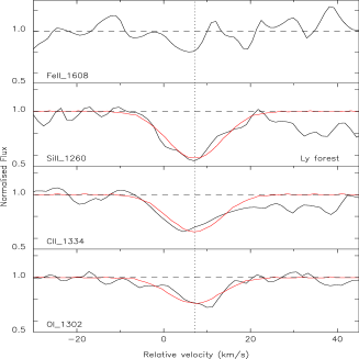
    Figure 16: Fit to the low-ionisation transitions of the $z_{\rm abs}$=3.665 $\log N_{\rm HI}$=19.11$\pm$0.10 sub-DLA towards BRI J0137$-$4224 (see Table 16). The region 25–25 km s^-1 is contaminated by an unidentified blend.

    Table 17: Parameters fit to the high-ionisation transitions of the $z_{\rm abs}$=3.665 $\log N_{\rm HI}$=19.11$\pm$0.10 sub-DLA towards BRI J0137$-$4224.

    z	$b$	log N($\rm Si~{}{\sc iv}$)
    3.665009	6.60$\pm$5.20	12.43$\pm$0.22
    3.665482	7.30$\pm$3.80	12.95$\pm$0.10

    

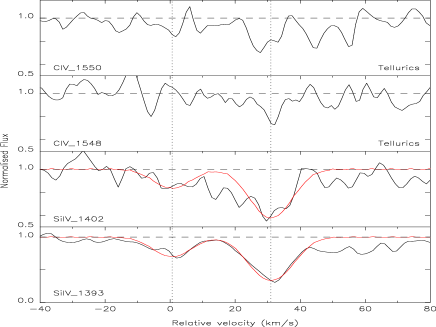
    Figure 17: Fit to the high-ionisation transitions of the $z_{\rm abs}$=3.665 $\log N_{\rm HI}$=19.11$\pm$0.10 sub-DLA towards BRI J0137$-$4224 (see Table 17).

11. BR J2215$-$1611 ($z_{\rm em}$=3.990, $z_{\rm abs}$=3.656, $\log N_{\rm HI}$=19.01$\pm$0.15):

    The two sub-DLAs detected towards BR J2215$-$1611 are essentially blended together and only come apart at the Lyman-$\gamma$ level. The first system at $z_{\rm abs}$=3.656 is also the weakest H i column density with $\log N_{\rm HI}$=19.01$\pm$0.15. Metal lines are seldom detected partly because of contamination with the Lyman-$\alpha$ forest lines. Few lines (Si ii $\lambda$ 1304, Si ii $\lambda$ 1526, Si ii $\lambda$ 1808 and Fe ii $\lambda$ 1608) fall in regions free from any contamination and yet remain undetected. We derive upper limits on the column densities of the corresponding ions: log N($\rm Si~{}{\sc ii}$)$<$14.41, log N($\rm Fe~{}{\sc ii}$)$<$13.51 and log N($\rm S~{}{\sc ii}$)$<$13.68. The intermediate ionisation transitions Al iii $\lambda$ 1854 and Al iii $\lambda$ 1862 are falling in the region polluted by telluric lines which prevent us from any detection or even determination of an upper limit.

    The high-ionisation transitions, C iv $\lambda$ 1548 and C iv $\lambda$ 1550, are detected in this system. To the immediate blue wavelength of the C iv $\lambda$ 1548 line lies a telluric line. The profile is well fitted by one component whose characteristics are derived from a simultaneous fit of the two members of the doublet, but only an upper limit is derived to be conservative. The $\rm Si~{}{\sc iv}$ in this sub-DLA is not detected although both lines are covered by our data. This leads to an upper limit on the column density: log N($\rm Si~{}{\sc iv}$)$<$11.69. The fit is shown in Figure 18 and the matching parameters are presented in Table 18.

    Table 18: Parameters fit to the high-ionisation transitions of the $z_{\rm abs}$=3.656 $\log N_{\rm HI}$=19.01$\pm$0.15 sub-DLA towards BR J2215$-$1611.

    z	$b$	log N($\rm C~{}{\sc iv}$)
    3.656415	33.30$\pm$16.86	$<$13.22

    

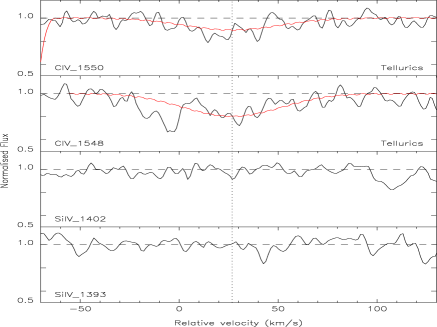
    Figure 18: Fit to the high-ionisation transitions of the $z_{\rm abs}$=3.656 $\log N_{\rm HI}$=19.01$\pm$0.15 sub-DLA towards BR J2215$-$1611 (see Table 18).

12. BR J2215$-$1611 ($z_{\rm em}$=3.990, $z_{\rm abs}$=3.662, $\log N_{\rm HI}$=20.05$\pm$0.15):

    Contrary to the previous system, this sub-DLA has a fairly high $N_{\rm HI}$ column density $\log N_{\rm HI}$=20.05$\pm$0.15 at $z_{\rm abs}$=3.662. It is characterised by strong metal lines showing a complex profile over $\sim$100 km s^-1. The 5 components are simultaneously fitted to O i $\lambda$ 1302, the un-saturated components of C ii $\lambda$ 1334, Al ii $\lambda$ 1670 and Si ii $\lambda$ 1526. The first component is narrower in Si ii $\lambda$ 1526 than in the other metal lines including Si ii $\lambda$ 1304. We note however that O i $\lambda$ 1302 is controversial and that it is a borderline case between a lower limit and a value.

    The resulting fit is applied to the other $\rm Si~{}{\sc ii}$ lines: Si ii $\lambda$ 1304 is clearly well fitted by this profile. Si ii $\lambda$ 1808 is not detected in agreement with our fit, while Si ii $\lambda$ 1190, Si ii $\lambda$ 1193 and Si ii $\lambda$ 1260 which are situated in the Lyman-$\alpha$ forest are clearly blended by other intervening lines. Nevertheless, the fit is found to be consistent with the upper limit they provide. All Fe ii $\lambda$ lines but Fe ii $\lambda$ 1125 are contaminated, but we use the non detection of Fe ii $\lambda$ 1125 to derive log N($\rm Fe~{}{\sc ii}$)$<$13.60. The fit is shown in Figure 19 and the matching parameters are presented in Table 19. The intermediate ionisation transitions Al iii $\lambda$ 1854 and Al iii $\lambda$ 1862 are falling in the region polluted by telluric lines which prevent us from any detection or even determination of an upper limit.

    The high-ionisation transitions in this system are well fitted with 3 components. The redshifts and $b$ of these were determined by a simultaneous fit of the C iv $\lambda$ 1548 and Si iv $\lambda$ 1402 lines. The fit is then superimposed on C iv $\lambda$ 1550 and Si iv $\lambda$ 1393. Clearly the Si iv $\lambda$ 1393 line is blended although no telluric lines are seen in this region. This fit leads accurate column density determinations. The fit is shown in Figure 20 and the matching parameters are presented in Table 20.

    Table 19: Parameters fit to the low-ionisation transitions of the $z_{\rm abs}$=3.662, $\log N_{\rm HI}$=20.05$\pm$0.15 sub-DLA towards BR J2215$-$1611.

    z	$b$	log N($\rm Si~{}{\sc ii}$)	log N($\rm C~{}{\sc ii}$)	log N($\rm O~{}{\sc i}$)	log N($\rm Al~{}{\sc ii}$)
    3.661105	3.30$\pm$0.10	12.95$\pm$0.28	13.72$\pm$0.48	14.03$\pm$0.01	11.70$\pm$0.16
    3.661597	6.80$\pm$0.10	13.45$\pm$0.02	$>$13.95	14.61$\pm$0.20	11.92$\pm$0.27
    3.661754	6.80$\pm$0.20	12.60$\pm$0.03	$>$13.35	13.61$\pm$0.02	11.47$\pm$0.10
    3.661885	5.10$\pm$0.10	13.38$\pm$0.01	14.81$\pm$0.20	14.25$\pm$0.01	11.95$\pm$0.67
    3.662193	3.50$\pm$0.10	13.11$\pm$0.02	$>$14.16	14.58$\pm$0.02	11.55$\pm$0.53

    

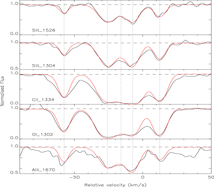
    Figure 19: Fit to the low-ionisation transitions of the $z_{\rm abs}$=3.662, $\log N_{\rm HI}$=20.05$\pm$0.15 sub-DLA towards BR J2215$-$1611 (see Table 19).

    Table 20: Parameters fit to the high-ionisation transitions of the $z_{\rm abs}$=3.662, $\log N_{\rm HI}$=20.05$\pm$0.15 sub-DLA towards BR J2215$-$1611.

    z	$b$	log N($\rm C~{}{\sc iv}$)	log N($\rm Si~{}{\sc iv}$)
    3.661409	7.20$\pm$ 5.00	12.79$\pm$0.07	12.67$\pm$0.08
    3.661881	12.40$\pm$ 3.10	13.57$\pm$0.25	13.39$\pm$0.04
    3.662255	26.50$\pm$ 8.80	12.92$\pm$0.08	12.53$\pm$0.07

    

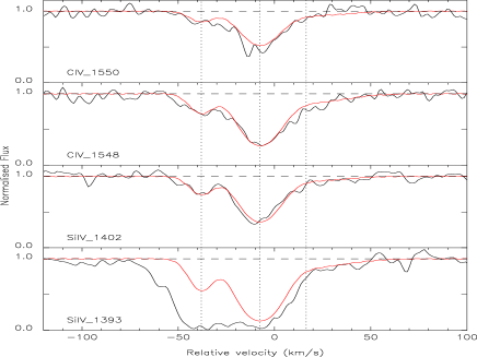
    Figure 20: Fit to the high-ionisation transitions of the $z_{\rm abs}$=3.662, $\log N_{\rm HI}$=20.05$\pm$0.15 sub-DLA towards BR J2215$-$1611 (see Table 20).

13. BR J2216$-$6714 ($z_{\rm em}$=4.469, $z_{\rm abs}$=3.368, $\log N_{\rm HI}$=19.80$\pm$0.10):

    This sub-DLA has a mid-range column density $\log N_{\rm HI}$=19.80$\pm$0.10 at $z_{\rm abs}$=3.368. Nevertheless, the low-ionisation transitions in this system are barely detected, partly because of Lyman-$\alpha$ contamination (the metal lines with $\lambda_{\rm rest}<$1522 Å in this sub-DLA will fall in the forest). This applies to many of the $\rm Si~{}{\sc iii}$ lines (Si ii $\lambda$ 1304, Si ii $\lambda$ 1260, Si ii $\lambda$ 1193, Si ii $\lambda$ 1190 and Si ii $\lambda$ 1526). The non-detection of Si ii $\lambda$ 1808 lead to the determination of an upper limit: log N($\rm Si~{}{\sc ii}$)$<$13.88 at 4$\sigma$. Similarly, most of the $\rm Fe~{}{\sc ii}$ lines are in the forest, but the region at the expected position of Fe ii $\lambda$ 1608 has a fairly high signal-to-noise leading to a constraining upper limit on the $\rm Fe~{}{\sc ii}$ column density: log N($\rm Fe~{}{\sc ii}$)$<$13.26. Al iii $\lambda$ 1854 and 1862 are also undetected: log N($\rm Al~{}{\sc iii}$)$<$11.51. On the contrary, a two component feature at the expected position of Al ii $\lambda$ 1670 is clearly detected. We compute an abundance determination for this element. The fit is shown in Figure 21 and the matching parameters are presented in Table 21.

    In addition, the high-ionisation transitions are also undoubtfully detected for this system. The $\rm C~{}{\sc iv}$ doublet is clearly detected and leads an accurate column density determination using a simultaneous fit of both members of the doublet to determine the redshifts and $b$ of 6 components. The $\rm Si~{}{\sc iv}$ doublet appears to be blended with Lyman-$\alpha$ forest interlopers, although Si iv $\lambda$ 1393 is most probably free form any contamination. The parameters derived from $\rm C~{}{\sc iv}$ are used to determine the upper limits on Si iv $\lambda$ 1393, but the first and fourth components are not detected in $\rm Si~{}{\sc iv}$. The fit is shown in Figure 22 and the matching parameters are presented in Table 22.

Table 21: Parameters fit to the low-ionisation transitions of the $z_{\rm abs}$=3.368, $\log N_{\rm HI}$=19.80$\pm$0.10 sub-DLA towards BR J2216$-$6714.

z	$b$	log N($\rm Al~{}{\sc ii}$)
3.369173	15.20$\pm$2.54	11.88$\pm$0.26
3.370053	17.40$\pm$3.04	11.85$\pm$0.27

Figure 21: Fit to the low-ionisation transitions of the $z_{\rm abs}$=3.368, $\log N_{\rm HI}$=19.80$\pm$0.10 sub-DLA towards BR J2216$-$6714 (see Table 21).

Table 22: Parameters fit to the high-ionisation transitions of the $z_{\rm abs}$=3.368, $\log N_{\rm HI}$=19.80$\pm$0.10 sub-DLA towards BR J2216$-$6714.

z	$b$	log N($\rm C~{}{\sc iv}$)	log N($\rm Si~{}{\sc iv}$)
3.368701	20.10$\pm$ 4.07	12.95$\pm$0.11	…∗
3.369287	15.50$\pm$ 2.96	13.02$\pm$0.12	$<$12.52
3.369919	12.60$\pm$ 5.42	13.01$\pm$0.09	$<$12.34
3.370177	6.10$\pm$ 1.99	12.58$\pm$0.22	…∗
3.370583	74.00$\pm$ 1.59	13.49$\pm$0.08	$<$13.09
3.370990	8.30$\pm$ 2.01	13.03$\pm$0.08	$<$12.48

^∗: These components are undetected in $\rm Si~{}{\sc iv}$.

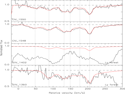
Figure 22: Fit to the high-ionisation transitions of the $z_{\rm abs}$=3.368, $\log N_{\rm HI}$=19.80$\pm$0.10 sub-DLA towards BR J2216$-$6714 (see Table 22).

3 Results

3.1 Individual Abundances

The resulting total column densities for each elements detected in the 13 sub-DLAs studied here are summarised in Table 23 together with the error estimates.

Table 23: Total column densities for each absorber.

Quasar	$z_{\rm abs}$	log N($\rm Fe~{}{\sc ii}$)	log N($\rm Si~{}{\sc ii}$)	log N($\rm C~{}{\sc ii}$)	log N($\rm O~{}{\sc i}$)	log N($\rm Al~{}{\sc ii}$)	log N($\rm Al~{}{\sc iii}$)	log N($\rm C~{}{\sc iv}$)	log N($\rm Si~{}{\sc iv}$)
PSS J0118$+$0320†	4.128	14.16$\pm$0.11	14.84$\pm$0.13	$>$17.30	$>$16.40	…	…	14.30$\pm$0.12	13.78$\pm$0.12
PSS J0121$+$0347	2.976	13.18$\pm$0.30	$<$13.15	$<$13.72	$<$13.98	11.93$\pm$0.32	$<$11.77∗	$<$13.79	13.33$\pm$0.10
SDSS J0124$+$0044†	2.988	$<$13.55+	14.12$\pm$0.12	$<$15.72	…	12.76$\pm$0.13	…	14.43$\pm$0.30	$<$14.20
…	3.078	$<$14.13	15.13$\pm$0.39	$>$15.35	$>$15.15	…	…	…	…
PSS J0133$+$0400	3.139	…	$<$13.14	$<$13.85	…	…	$<$11.44∗	…	…
…	3.995	$<$13.56∗@	13.91$\pm$0.13	…	…	$<$11.36∗	$<$11.69∗	$<$13.51	13.48$\pm$0.28
…	3.999	$<$13.56∗	$<$14.12∗	…	…	$<$11.10∗	$<$11.63∗	$<$13.76	$<$13.25
…	4.021	$<$13.56∗	$<$14.05∗	…	…	$<$11.20∗	…	$<$12.31∗	$<$12.89
BRI J0137$-$4224	3.101	13.67$\pm$0.11	14.11$\pm$0.25	…	…	12.83$\pm$0.42	…	13.52$\pm$0.17	…
…	3.665	$<$13.59∗	12.40$\pm$0.13	13.14$\pm$0.13	13.38$\pm$0.13	$<$11.06∗	$<$11.96∗	$<$12.11∗	13.06$\pm$0.13
BR J2215$-$1611†	3.656	$<$13.51∗	$<$14.41∗	…	…	…	…	$<$13.22	$<$11.69∗
…	3.662	$<$13.60∗	13.89$\pm$0.06	$>$14.98	15.05$\pm$0.02	12.46$\pm$0.45	…	13.71$\pm$0.21	13.51$\pm$0.05
BR J2216$-$6714	3.368	$<$13.26∗	$<$13.88∗	…	…	12.17$\pm$0.26	$<$11.51∗	13.88$\pm$0.10	$<$13.32

^∗: 4 $\sigma$ upper limits corresponding to non-detections

⁺: log N($\rm Fe~{}{\sc iii}$)$<$14.09 in this system

^@: log N($\rm Ni~{}{\sc ii}$)$<$12.31 in this system from a non-detection

^†: PSS J0118$+$0320, $z_{\rm abs}$=4.128 has log N($\rm S~{}{\sc ii}$)=14.26$\pm$0.11, SDSS J0124$+$0044, $z_{\rm abs}$=2.988 has log N($\rm S~{}{\sc ii}$)$<$14.27, BR J2215$-$1611, $z_{\rm abs}$=3.656 has log N($\rm S~{}{\sc ii}$)$<$13.68 from a non-detection.

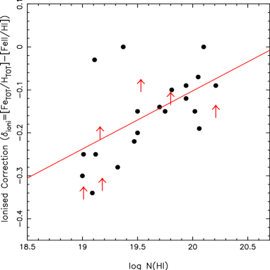
Figure 23: Ionisation correction, $\delta_{ioni}$, as a function of $\log N_{\rm HI}$ from the present study and from the literature (Prochaska et al. 1999; Dessauges-Zavadsky et al. 2003; Péroux et al. 2006a; Prochaska et al. 2006). There seems to be trend of smaller ionisation corrections towards higher $N_{\rm HI}$, as expected. The solid line is the linear least squares regression with slope $\alpha=0.13$. Note that in most cases, the correction, $\delta_{ioni}$, is smaller than 0.2 dex.

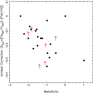
Figure 24: Ionisation correction, $\delta_{ioni}$, as a function of observed metallicity, [Fe/H] (or [Si/H] when Fe measurements are not available). There is a hint of decreasing $\delta_{ioni}$ with metallicity.

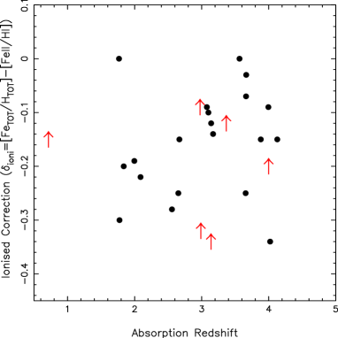
Figure 25: Ionisation correction, $\delta_{ioni}$, as a function of absorption redshift. Given than the incident UV background flux evolves with redshift, a correlation of the ionisation corrections with $z_{\rm abs}$ is expected. No such correlation is observed.

One concern is that sub-DLAs may be partially ionised in H, in which case the observed $\rm Fe~{}{\sc ii}$ to H i ratio would not be a good measure of the total Fe abundance for instance. Indeed, given that $\rm Fe~{}{\sc ii}$ has an ionisation potential, IP(FeII)=16.18eV, larger than hydrogen, IP(HI)=13.59eV, some of the observed $\rm Fe~{}{\sc ii}$ could reside in the ionised gas of the sub-DLA with lower $N_{\rm HI}$. This leads to a slight overestimate of the true total metallicity of the systems. To investigate the ionisation corrections, we compute photo-ionisation models based on the CLOUDY software package (version 94.00, Ferland 1997), assuming ionisation equilibrium and a solar abundance pattern. Based on the modelling of 13 systems, Dessauges-Zavadsky et al. (2003) have shown that differences between a Haardt-Madau or a stellar-like spectrum are negligible. Here, we chose to perform the modelling using a stellar-like incident ionisation spectrum (D’Odorico & Petitjean 2001). We thus obtain the theoretical column density predictions for any ionisation state of all observed ions as a function of the ionisation parameter $U$. When possible, we then use observed ratios of the same element in different states (i.e. $\rm Fe~{}{\sc ii}$/$\rm Fe~{}{\sc iii}$, $\rm Al~{}{\sc ii}$/$\rm Al~{}{\sc iii}$, $\rm Si~{}{\sc iii}$/$\rm Si~{}{\sc iv}$ or $\rm C~{}{\sc ii}$/$\rm C~{}{\sc iv}$) and compare them with predictions from the model to constrain the $U$ parameter. When only limits on the $U$ parameter were available, we have established a limit on the ionisation correction. Moreover, on two occasions, such ratios are not available and the observed column densities are directly compared with the predicted ones to deduce the $U$ parameter.

Once the ionisation parameter $U$ is known, we can deduce by how much the observed metallicity, $FeII_{obs}/HI_{obs}$, deviates from the total metallicity, $Fe_{TOT}/H_{TOT}$ of the absorber. We compute the correction to bring to the observed $\rm Fe~{}{\sc ii}$ values, the so-called $\delta_{ioni}$ as follows:

$$\delta_{ioni}=\frac{Fe_{TOT}}{H_{TOT}}-\frac{FeII_{obs}}{HI_{obs}}$$ (1)

A negative (positive) $\delta_{ioni}$ corresponds to an overestimate (underestimate) of the total metallicity. Figure 23 shows the correction for 26 sub-DLAs as function of $N_{\rm HI}$ column densities from the present study and from the literature (Prochaska et al. 1999; Dessauges-Zavadsky et al. 2003; Péroux et al. 2006a; Prochaska et al. 2006). Recent findings by Fox et al. (2007) on the ionised fraction in O and C of a sample of DLAs are also in line with the present results. The solid line is a fit to the measures (as opposed to lower limits) with slope $\alpha$=0.13. As in Dessauges-Zavadsky et al. (2003) and more recently, Prochaska et al. (2006), we find that the ionisation correction for sub-DLAs are small and within the error estimates in most cases (sse also Erni et al. 2006 for a borderline case). In the present study, only 4 sub-DLAs out of the 13 studied require a correction $|\delta_{ioni}|>0.2$ dex. In all these 4 cases, the correction is $|\delta_{ioni}|<0.35$ dex. The $\delta_{ioni}$ values for each sub-DLAs are listed in Table 24. There is a hint of decreasing $\delta_{ioni}$ with metallicity (Figure 24). Knowing that sub-DLAs are more metal-rich than classical DLAs (Kulkarni et al. 2007), possibly due to an observational bias, and that the ionisation correction increases with decreasing $N_{\rm HI}$ (see Figure 23); it is no surprise to observe that the ionisation correction gets larger as the metallicity gets higher. It is interesting to note however that the fractional correction remains roughly constant. However, no clear correlation of $\delta_{ioni}$ with absorption redshift is detected (Figure 25), contrary to what one would expect from the redshift evolution of the incident UV background photons.

The total absolute abundances were calculated with respect to solar using the following formula:

$$[X/H]=\log[N(X)/N(H)]_{DLA}-\log[N(X)/N(H)]_{\odot}$$ (2)

where $\log[N(X)/N(H)]_{\odot}$ is the solar abundance and is taken from Asplund et al. (2005) adopting the mean of photospheric and meteoritic values for Fe, Si, C, O, S and Al. These values are recalled on the top line of Table 24.

Table 24: Abundances with respect to solar, [X/H], using the standard definition: $[X/H]=\log[N(X)/N(H)]_{DLA}-\log[N(X)/N(H)]_{\odot}$. The error bars on [X/H] include both the errors in log $N(X)$ and $\log N_{\rm HI}$. $\delta_{ioni}$ is the correction to the observed metallicity required to take into account the ionised part gas (see equation 1).

Quasar	$z_{\rm abs}$	$\log N_{\rm HI}$	Fe	$\delta_{ioni}$	Si	C	O	S	Al
A(X/N)☉	–	–	$-$4.55	–	$-$4.49	$-$4.10	$-$3.47	$-$4.85	$-$5.60
PSS J0118$+$0320	4.128	20.02$\pm$0.15	$-$1.31$\pm$0.26	$-$0.15	$-$0.69$\pm$0.28	$>$1.38	$>-$0.15	$-$0.91$\pm$0.26	…
PSS J0121$+$0347	2.976	19.53$\pm$0.10	$-$1.80$\pm$0.40	$<|-$0.09$|$	$<-$1.89	$<-$1.71	$<-$2.08	…	$-$2.00$\pm$0.42
SDSS J0124$+$0044	2.988	19.18$\pm$0.10	$<-$1.08	$<|-$0.32$|$	$-$0.57$\pm$0.22	$<$0.64	…	$<-$0.06	$-$0.82$\pm$0.23
…	3.078	20.21$\pm$0.10	$<-$1.53	$-$0.09	$-$0.59$\pm$0.49	$>-$0.76	$>-$1.59	…	…
PSS J0133$+$0400	3.139	19.01$\pm$0.10	…	$<|-$0.34$|$	$<-$1.38	$<-$1.06	…	…	…
…	3.995	19.94$\pm$0.15	$<-$1.83	$-$0.09	$-$1.54$\pm$0.28	…	…	…	$<-$2.98
…	3.999	19.16$\pm$0.15	$<-$1.05	$<|-$0.20$|$	$<-$0.55	…	…	…	$<-$2.46
…	4.021	19.09$\pm$0.15	$<-$0.98	$-$0.34	$<-$0.55	…	…	…	$<-$2.29
BRI J0137$-$4224	3.101	19.81$\pm$0.10	$-$1.59$\pm$0.21	$-$0.10	$-$1.21$\pm$0.35	…	…	…	$-$1.38$\pm$0.52
…	3.665	19.11$\pm$0.10	$<-$0.97	$-$0.03	$-$2.22$\pm$0.23	$-$1.87$\pm$0.23	$-$2.26$\pm$0.23	…	$<-$2.45
BR J2215$-$1611	3.656	19.01$\pm$0.15	$<-$0.95	$-$0.25	$<-$0.11	…	…	$<-$0.48	…
…	3.662	20.05$\pm$0.15	$<-$1.90	$-$0.07	$-$1.67$\pm$0.21	$>-$0.97	$-$1.53$\pm$0.17	…	$-$1.99$\pm$0.60
BR J2216$-$6714	3.368	19.80$\pm$0.10	$<-$1.99	$<|-$0.12$|$	$<-$1.43	…	…	…	$-$2.03$\pm$0.36

3.2 Global Metallicity

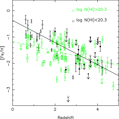
Figure 26: Redshift evolution of [Fe/H] metallicity in DLAs and sub-DLAs. Filled circles are sub-DLAs studied by our group (Dessauges-Zavadsky et al. 2003 and the present study). Sub-DLAs are found to evolve more with time than DLAs, and to be more metal-rich at the lowest redshifts. The lines show the least square regressions fitted to the data (excluding limits) for DLAs (dashed line) and sub-DLAs (solid line).

Figure 26 shows the resulting redshift evolution of the metallicity of DLAs and sub-DLAs including our new sample of 13 high-redshift sub-DLAs. The data plotted are based on Péroux et al. (2003b) compilation with the following studies added: Dessauges-Zavadsky, et al. (2004), Rao et al. (2005), Péroux et al. (2006a), Péroux et al. (2006b) and Meiring et al. (2007). We note that thanks to these recent studies the metallicity of sub-DLAs is now better constrained. These results confirm findings from Péroux et al. (2003b) that the average values of the metallicities in the different redshift bins do show more evolution with redshift in the case of sub-DLA than for classical DLAs. Fitting least square regressions to the data points without including limits lead to a slope of $\alpha=-0.18$ for DLAs and $\alpha=-0.42$ for sub-DLAs. These regression fits are plotted as dashed and solid lines (respectively) on Figure 26. Moreover, based on Zn measurements, sub-DLAs appear more metal-rich at lower redshifts, specially at $z<2$ (Péroux et al. 2006a; Péroux et al. 2006b, Meiring et al. 2007). Although our data add no new Zn measurements because of their high-redshifts, it has been previously shown (Péroux et al. 2003b) that the strong evolution observed in [Fe/H] for sub-DLAs is not due to differential depletion given that such strong evolution is also observed in [Zn/H] metallicity of sub-DLAs.

Rather, the difference in evolution might be explained by the fact that sub-DLAs are less prone to the biasing effect of dust and thus represent a better tool to detect the most metal-rich galaxies seen in absorption. Indeed, it has been suggested that the dust contained in the absorbers might introduce biases into current surveys in the sense that the dustier systems would dim the light from the background quasar and therefore not be taken into account in current magnitude-limited samples. In order to overcome such limitations, searches for DLAs towards radio-selected quasars have been undertook and their results suggest that dust obscuration might be modest (Ellison et al. 2001; Jorgenson et al. 2006). However, the samples are still small to derive firm conclusions and some of the radio-selected quasars are actually “dark” at optical wavelengths and can thus potentially be obscured quasars. In fact, if dust extinction in quasar absorbers is a strong function of N($\rm Zn~{}{\sc ii}$) column density as found in interstellar clouds (Vladilo et al. 2004), the obscuration will start acting at a lower [Zn/H] ratio for DLAs than for sub-DLAs (Vladilo & Péroux, 2005). In other words, we might be missing more systems in the DLA range than in the sub-DLA range and the metal-rich sub-DLAs recently found would be the “tip of the iceberg” population which has remained so far un-noticed. A way to find metal-rich absorbers minimising dust effects is therefore to search for quasar absorbers with relatively lower $N_{\rm HI}$ column density such as the sub-DLAs. Another possibility to explain the metallicity difference between DLAs and sub-DLAs has recently been suggested by Khare et al. (2006). Based on the observed mass-metallicity relationship for galaxies (e.g. Tremonti et al. 2004; Savaglio et al. 2005), the authors argue that sub-DLAs may arise in massive galaxies and DLAs in less massive galaxies.

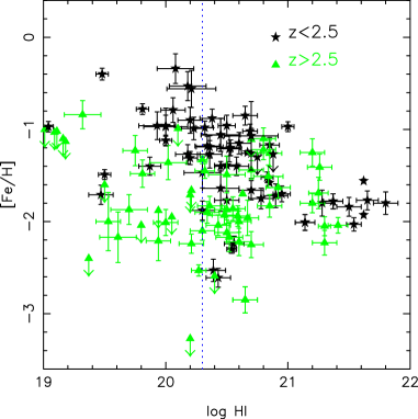
Figure 27: [Fe/H] metallicity of both DLAs and sub-DLAs as a function of $\log N_{\rm HI}$. The dotted vertical line corresponds to the DLA definition: log $N_{\rm HI}$$>20.3$. Different redshift ranges are symbol+colour coded and show once more the fastest redshift-evolution of sub-DLAs with respect to DLAs.

In Figure 27, the metallicity of both DLAs and sub-DLAs is shown as a function of $\log N_{\rm HI}$. The spread in metallicity is larger in the sub-DLAs range showing once more a strong evolution with redshift, while classical DLAs appear more homogeneous.

4 Discussion

4.1 The Missing Metals Problem

A direct consequence of the star formation history is the production of heavy elements, known as metals. However, at high-redshift, our knowledge of the cosmic metal budget is still highly incomplete. In fact, the amount of metals observed in high-redshift galaxies (e.g. Lyman-Break Galaxies, DLAs) and the intergalactic medium, was believed to be roughly a factor of 5 below the expected amount of metals produced as a result of the cosmic star formation history. This is dubbed as the “missing metals problem” (Pettini 1999 and Pettini 2004). This census has recently been revisited in a series of papers, which explore alternative populations which might also contain part of the missing metals. Bouché, Lehnert & Péroux (2005) have investigated the role of sub-mm galaxies while Bouché, Lehnert & Péroux (2006) have considered the Lyman-Break Galaxies. But a substantial fraction of the missing metals may also be hidden in a very hot, collisionally ionised gas (Ferrara et al. 2005). Based on simple order-of-magnitude calculations, Bouché et al. (2007) discuss the possibility that the remaining missing metals could have been ejected from small galaxies via galactic outflows into the intergalactic medium in a hot phase which is difficult to detect using observed properties of local galaxies. However, even when taking into account the most recent observations, it appears that 10 to 40% of metals are still missing.

Although we can measure the metallicities of DLAs up to high-redshifts, the above studies find that their ad-hoc metallicities is too low for them to be a major contributor to the metal budget. However, Davé & Oppenheimer (2007) used cosmological hydrodynamic simulations based on GADGET-2 to compute the redshift evolution and contribution of DLAs to the metal census. They find that their simulations reproduce well the mild redshift evolution observed in DLAs but overproduce the metallicity at all redshifts. They suggest that highly enriched sub-DLAs might accommodate for the discrepancy. In the following, we use the most recent observational data on sub-DLAs to calculate their contribution to the metal budget.

4.2 Contribution of Sub-DLAs to the Global Metallicity

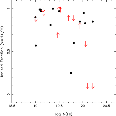
Figure 28: Ionised fraction, $x=H^{+}/H_{TOT}$, of a sample of 26 sub-DLAs as a function of $N_{\rm HI}$ column densities. The up and down arrows denote lower and upper limits, respectively. Note that a number of $x$ values are found at any given $N_{\rm HI}$ column density (see for example $N_{\rm HI}$$\sim$19.7).

Recently, there have been several attempts to estimate the amount of metals contained in sub-DLAs (Prochaska et al. 2006), including some results based on dust-free Zn metallicities measures (Kulkarni et al. 2006). Indeed, Pettini (2006) has suggested that some of the missing metals might be in sub-DLAs if those were to have a significant ionised fraction. But the amount of metals in the ionised gas of sub-DLAs cannot be directly probed by observations. In fact, it is interesting to note that Lebouteiller et al. (2006) have recently shown that the ionised gas probed in emission is more metal-rich that the neutral gas probed in absorption for most elements in a local HII region. While the reasons for this is not yet clear, they also note that $\rm Fe~{}{\sc ii}$ is a better tracer of neutral gas than $\rm Si~{}{\sc iii}$.

For high-redshift quasar absorbers, the only mean to quantify the ionised fraction is to use photo-ionisation models. The ionised fraction is defined as:

$x=H^{+}/H_{TOT}$

Prochaska et al. (2006) estimate $x$=0.90 for one sub-DLA and compute $\Omega_{Z}(sub-DLAs)$ using this value. Here, we use the models presented in Section 3.1, to reproduce the ionisation state of 26 sub-DLAs. The $x$ values for these are shown in Figure 28 as a function of $N_{\rm HI}$ column densities. A range of $x$ values are found at any given $N_{\rm HI}$ column densities. Figure 29 shows the evolution of the ionisation fraction with metallicity for the 26 sub-DLAs studied. No obvious trend is observed.

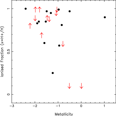
Figure 29: Evolution of the ionised fraction, $x$, with the metallicity, [Fe/H] (or [Si/H] when Fe measurements are not available). No obvious trend is observed.

At $z\sim$2.5, the amount of HI gas in sub-DLAs is measured to be $\Omega_{\rm HI}$=0.18 $\times$ 10^-3 (Péroux et al. 2005). At the same redshifts, the metallicity of these systems is measured from the undepleted Zn element is $Z/Z_{\odot}$=$-$0.70 (Kulkarni et al. 2007). The mean of $x$-values (as opposed to limits) at $z\sim$2.5 is $<x>=0.68$. Therefore, assuming all the gas is photo-ionised, the observed comoving mass density of metals in sub-DLAs is:

$$\Omega_{Z}(sub-DLAs)=\left(\frac{<x>}{1-<x>}+1\right)\times 10^{-0.70}\times 0.18\times 10^{-3}\times\frac{Z_{\odot}}{\Omega(Z_{\odot})}$$ (3)

$$\Omega_{Z}(sub-DLAs)=2.57\times 10^{-3}$$ (4)

where $Z_{\odot}$=0.0126 by mass and $\Omega(Z_{\odot})=\Omega_{\rm baryons}\times Z_{\odot}=5.5\times 10^{-4}$.

The total amount of metals expected at this redshift is $\Omega(Z)=4.5\times 10^{-2}$. Therefore, the sub-DLAs are contributing at most $\sim$ 6% of the total metal in the Universe at $z\sim 2.5$ for a photo-ionised gas. According to recent results, if the gas was collisionally ionised, the contribution to the total amount of metals would be similar (Fox et al.2007). So, even if sub-DLAs are mostly ionised gas, they do not close the metal budget. In fact, given that 10 to 40% of the metals are still missing, the mean metallicity of sub-DLAs after ionisation correction should be $-0.46<Z/Z_{\odot}<+0.14$ for these systems to close the missing metals problem. Such metal-rich galaxies would be easily observed in emission. This is not the case of quasar absorbers which probably trace fainter objects. Note that the higher the ionised fraction of sub-DLAs, $x$, the higher is their contribution to the cosmic metallicity. It will thus be very important in the future to measure the ionised fraction of more sub-DLAs, to better constrain $<x>$ at $z\sim$2.5.

4.3 Redshift Evolution of the Ionised Fraction

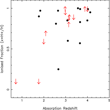
Figure 30: Evolution with cosmic time of the ionised fraction, $x$, in sub-DLAs.

Figure 30 shows the evolution with cosmic time of the ionised fraction in sub-DLAs. Clearly, one would expect the ionised fraction of sub-DLA to increase with cosmic times as the Universe becomes ionised and the meta-galactic flux increases up to z=1.5. On the contrary, no clear trend seems to appear with redshift. This result supports the picture where sub-DLAs are a phase of galaxy evolution observed at various redshifts rather than a tracer of the continuous formation of galaxies and/or that we are probing different overdensities at different redshifts. In fact, systems which are more affected by higher ultra-violet flux probably have a lower observed $N_{\rm HI}$ and are therefore not classified as sub-DLAs. Indeed, the gas cooling time is expected to be $\sim$ 10⁹ yrs, i.e. much longer than the time it takes for H i to turn into stars ($\sim$ 10⁷ yrs) or to be heated by the meta-galactic flux. This also goes in line with the fact that only small amounts of molecular hydrogen H₂ are found in quasar absorbers (Srianand et al. 2005, Zwaan & Prochaska 2006).

5 Summary

We have presented abundance and ionisation fraction determinations of a sample of 13 $z\geq 3$ sub-DLAs. In summary:

• our new high-resolution observations more than double the metallicity information for sub-DLAs previously available at $z>3$.

• results from photo-ionisation modellings of a sample of 26 sub-DLAs are put together for the first time.

• the ionisation correction to the observed metallicity, $\delta_{ioni}$ is a function of the observed $N_{\rm HI}$ column density and smaller than 0.2 dex in most cases.

• the metallicity of sub-DLA evolves faster with cosmic times than the one of classical DLAs and is higher especially at $z<2$. This could be due to sub-DLAs being less affected by the biasing effect of dust.

• the ionisation fraction of a sample of 26 sub-DLAs allows to reliably calculate the total contribution of these systems to the so-called “missing metals problem”. Sub-DLAs contribute no more than 6% of the total amount of expected metals at z$\sim$2.5.

6 Acknowledgments

We would like to thank Valentina D’Odorico for providing the raw spectrum of PSS J0133$+$0400 860 setting in advance of publication.

References

- [1] Asplund, M., Grevesse, N., & Sauval, A. J., ASP Conference Series, 2005, Ed Bash & Barnes, 336, 25.
- [2] Bouché, N., Lehnert, M. D. & Péroux, C., 2005, MNRAS, 364, 319
- [3] Bouché, N., Lehnert, M. D. & Péroux, C., 2006, MNRAS, 367L, 16
- [4] Bouché, N., Lehnert, M. D., Aguirre, A., Péroux, C. & Bergeron, J., 2007, MNRAS, 378, 525
- [5] Davé, R.& Oppenheimer, B. D., 2007, MNRAS, 374, 427.
- [6] Dessauges-Zavadsky, M., Péroux, C., Kim, T.S., D’Odorico, S., & McMahon, R.G., 2003, MNRAS, 345, 447.
- [7] Dessauges-Zavadsky, M., Calura, F., Prochaska, J. X., D’Odorico, S. & Matteucci, F., 2004, A&A, 416, 79
- [8] D’Odorico, V. & Petitjean, P., 2001, A&A, 370, 729
- [9] Ellison, S. L., Yan, L., Hook, I. M., Pettini, M., Wall, J. V., & Shaver, P., 2001, A&A, 379, 393.
- [10] Erni, P., Richter, P., Ledoux C. & Petitjean, P., 2006, A&A, 451, 19.
- [] Ferland, G.J., 1997, Hazy, a brief introduction to CLOUDY
- [] Ferrara, A., Scannapieco, E. & Bergeron, J., 2005, ApJL, 634, 37
- [] Fontana, A. & Ballester, P., 1995, Messenger, 80, 37.
- [] Fox, A., J., Petitjean, P., Ledoux, C. & Srianand, R., 2007, A&A, 465,171.
- [] Jenkins, E. B., Bowen, D. V., Tripp, T. M. & Sembach, K. R., 2005, ApJ, 623, 767
- [] Jorgenson, R. A., Wolfe, A. M., Prochaska, J. X., Lu, L., Howk, J. C., Cooke, J., Gawiser, E. & Gelino, D. M., 2006, ApJ, 646, 730
- [11] Khare, P., Kulkarni, V. P., Péroux, C., York, D. G., Lauroesch, J. T. & Meiring, J. D., 2007, A&A, 464, 487.
- [12] Kulkarni, V. P., Khare, P., Péroux, C., York, D. G., Lauroesch, J. T. & Meiring, J. D., 2007, ApJ, 661, 88.
- [13] Lebouteiller, V., Kunth, D., Lequeux, J., Aloisi, A., Desert, J.-M., Hebrard, G., Lecavelier des Etangs, A. & Vidal-Madjar, A., 2006, A&A, 459, 161.
- [14] Meiring, J. D., Lauroesch, J. T., Kulkarni, V. P., Péroux, C., Khare, P., York, D. G. & Crotts, A. P. S., 2007, MNRAS, 376, 557.
- [15] Péroux, C., McMahon, R., Storrie-Lombardi, L. & Irwin, M., 2003a, MNRAS, 346, 1103.
- [16] Péroux, C., Dessauges-Zavadsky, M., D’Odorico, S., Kim,T.S., & McMahon, R., 2003b, MNRAS, 345, 480.
- [17] Péroux, C., Dessauges-Zavadsky, M., D’Odorico, S., Kim, T. S.& McMahon, R. G., 2005, MNRAS, 363, 479.
- [18] Péroux, C., Kulkarni, V. P., Meiring, J., Ferlet, R., Khare, P., Lauroesch, J. T., Vladilo, G. & York, D. G., 2006a, A&A, 450, 53
- [19] Péroux, C., Meiring, J., Kulkarni, V. P., Ferlet, R., Khare, P., Lauroesch, J. T., Vladilo, G. & York, D. G., 2006b, MNRAS, 372, 369
- [20] Pettini, M., 1999, ‘Chemical Evolution from Zero to High Redshift’, Proceedings of the ESO Workshop held at Garching, Germany, 14-16 October 1998. Edited by Jeremy R. Walsh, Michael R. Rosa.
- [] Pettini, M., Ellison, S. L., Steidel, C. C., Shapley, A. E. & Bowen, D. V., 2000, ApJ, 532, 65.
- [21] Pettini, M., 2004, Canary Islands Winter School of Astrophysics, ‘Cosmochemistry: The Melting Pot of Elements’, edited by C. Esteban, R. J. Garcĩa López, A. Herrero, F. Sànchez.
- [22] Pettini, M., 2006, ‘The Fabulous Destiny of Galaxies: Bridging Past and Present’, eds. V. Le Brun, A. Mazure, S. Arnouts, & D. Burgarella.
- [23] Prochaska, J. X.,O’Meara, J. M., Herbert-Fort, S., Burles, S., Prochter, G. E. & Bernstein, R. A., 2006, ApJ, 648L, 97
- [24] Rao, S. M., Prochaska, J. X., Howk, J. C., Wolfe, A. M., 2005, AJ, 129, 9
- [25] Savaglio, S. et al., 2005, ApJ, 635, 260
- [26] Srianand, R., Petitjean, P., Ledoux, C., Ferland, G. & Shaw, G., 2005, MNRAS, 362, 549
- [27] Tremonti, C. et al., 2004, ApJ, 613, 898
- [28] Vladilo, G., 2004, A&A, 421, 479
- [29] Vladilo, G. & Péroux, C., 2005, A&A, , A&A, 444, 461.
- [30] Wolfe, A., Lanzetta, K. M., Foltz, C. B. & Chaffee, F. H., 1995, ApJ, 454, 698.
- [31] Zwaan, M. & Prochaska, J., 2006, ApJ, 643, 675