Faxén relations in solids - a generalized approach to particle motion in elasticity and viscoelasticity

Abstract

A movable inclusion in an elastic material oscillates as a rigid body with six degrees of freedom. Displacement/rotation and force/moment tensors which express the motion of the inclusion in terms of the displacement and force at arbitrary exterior points are introduced. Using reciprocity arguments two general identities are derived relating these tensors. Applications of the identities to spherical particles provide several new results, including simple expressions for the force and moment on the particle due to plane wave excitation.

1 Introduction

Faxén relations are named after Hilding Faxén who derived several identities for calculating hydrodynamic forces and torques on particles in low Reynolds number flows, e.g. Ref.  Faxen27. As an example of a Faxén relation, or law, the force and torque on a rigid sphere of radius $a$ moving with velocity ${\mbox{\boldmath$\displaystyle\mathbf{v}$}}_{0}$ and spinning with angular velocity $\displaystyle\mathbf{\omega}$ in an unbounded fluid of viscosity $\mu$ and velocity field ${\mbox{\boldmath$\displaystyle\mathbf{v}$}}({\mbox{\boldmath$\displaystyle\mathbf{r}$}})$ in the absence of the sphere are [Eqs. (3-2.46) and (3-2.47) of Ref.  Happel91]

$$\mathbf{F} =6\pi\mu a\big{[}{\mbox{\boldmath$\displaystyle\mathbf{v}$}}({\mbox{\boldmath$\displaystyle\mathbf{0}$}})-{\mbox{\boldmath$\displaystyle\mathbf{v}$}}_{0}\big{]}+\pi\mu a^{3}\nabla^{2}{\mbox{\boldmath$\displaystyle\mathbf{v}$}}({\mbox{\boldmath$\displaystyle\mathbf{0}$}}),$$ (1a)

$$\mathbf{T} =4\pi\mu a^{3}\big{[}\operatorname{curl}{\mbox{\boldmath$\displaystyle\mathbf{v}$}}({\mbox{\boldmath$\displaystyle\mathbf{0}$}})-2{\mbox{\boldmath$\displaystyle\mathbf{\omega}$}}\big{]}.$$ (1b)

The reader will note that the identities have as a special case the classical Stokes drag law, but they include additional effects caused by spatially variable flow fields. These and other Faxén relations for non-spherical particles are based upon general integral identities relating the force and torque on the particle to the external flow field Happel and Brenner (1991); Kim and Karilla (1991); Pozrikidis (1997). Although Faxén relations are commonly used in hydrodynamics and microfluidics, they seem to be essentially unknown outside that subject area. For instance, I am aware of only one mention(Phan-Thien and Kim, 1994) of a Faxén type relation in elasticity and that one was is in regards to elastostatics.

The objective of this paper is to develop similar ideas in the context of elastodynamics and in the process demonstrate their utility and wide application. Using dynamic reciprocity, a set of relations are first derived between the velocity or force of a particle in a solid matrix and the displacement or force at a distant point in the solid. These equations include but go far beyond the notion of particle impedance, which relates the force on a particle to its velocity. Numerous applications of the general relations are obtained by considering spherical particles. Faxén-like relations are derived for the force and moment on a spherical particle caused by plane wave incidence. Like their hydrodynamic counterparts, the elastodynamic Faxén relations are simple in form.

The analysis here is the second in a series of papers developing a simplified algebra for calculating the radiation and scattering from inclusions in elastic and viscoelastic materials. In the previous paper (Norris, 2006) the forced motion of a spherical particle in an elastic matrix was considered. Although this is a classical problem, originally solved by Oestreicher Oestreicher (1951), it turns out that the dynamic impedance of the inclusion can be represented in a simplified manner. This was achieved Norris (2006) through several lumped mass impedances for a spherical inclusion, in terms of which impedance or its inverse, admittance, has a simple form. The purpose of the present paper is to develop these ideas further, focusing on the interaction between the inclusion and remote points in the matrix.

The plan of the paper is as follows. The dynamic properties of an inclusion are defined in Section 2, as well as some important quantities that are used throughout the paper: the displacement/rotation tensors $\displaystyle\mathbf{U}$ and $\displaystyle\mathbf{W}$, the force/moment tensors $\displaystyle\mathbf{\Phi}$ and $\displaystyle\mathbf{\Psi}$, and the impedances $\displaystyle\mathbf{Z}$ and $\widetilde{\mbox{\boldmath$\displaystyle\mathbf{Z}$}}$. In Section 3 we prove the symmetry of these impedances, and derive two fundamental relations between the displacement/rotation and force/moment tensors. The remainder of the paper focuses on the special case of spherical inclusions. The fundamental quantities for the spherical particle are presented in Section 4 in a concise format using lumped mass impedances. Section 5 is the longest in the paper, as it contains numerous applications, discussion of limiting cases, and the new elastodynamic Faxén relations that are analogous to the classic hydrodynamic identities. The many results and their import are summarized in Section 6.

Regarding notation, the time harmonic factor $e^{-i\omega t}$ is omitted but understood. Boldface quantities are either vectors or second order tensors. Vectors are usually denoted by lower case, and tensors are capitalized, with the exceptions $\displaystyle\mathbf{F}$ and $\displaystyle\mathbf{M}$ which indicate force and moment vectors, respectively. The axial tensor $\operatorname{axt}({\mbox{\boldmath$\displaystyle\mathbf{a}$}})$ of the vector $\displaystyle\mathbf{a}$ is a skew symmetric tensor defined by $\operatorname{axt}({\mbox{\boldmath$\displaystyle\mathbf{a}$}}){\mbox{\boldmath$\displaystyle\mathbf{b}$}}={\mbox{\boldmath$\displaystyle\mathbf{a}$}}\wedge{\mbox{\boldmath$\displaystyle\mathbf{b}$}}$.

2 Inclusions and rigid body motion

An inclusion in a solid matrix is defined to be the surface $\partial V_{p}$ of a finite volume $V_{p}$ within which there could be a particle, or there could be some complicated “black box” with its own internal dynamics. The key feature of the inclusion is that its boundary $\partial V_{p}$ undergoes rigid body motion. In this sense the boundary is a rigid interface between the particle, whatever that may be, and the solid matrix. The term inclusion rather than particle is used throughout in order to remind us of this distinction.

2.1 Tensor functions $\displaystyle\mathbf{U}$, $\displaystyle\mathbf{W}$, $\displaystyle\mathbf{\Phi}$ and $\displaystyle\mathbf{\Psi}$

Rigid body motion has six degrees of freedom, which we characterize by two vector quantities: ${\mbox{\boldmath$\displaystyle\mathbf{u}$}}_{p}$ and ${\mbox{\boldmath$\displaystyle\mathbf{\theta}$}}_{p}$. ${\mbox{\boldmath$\displaystyle\mathbf{u}$}}_{p}$ is the rigid body displacement of the inclusion center of mass. ${\mbox{\boldmath$\displaystyle\mathbf{\theta}$}}_{p}$ describes the rotation of the inclusion about the center of mass. The most general displacement possible for the inclusion is

$${\mbox{\boldmath$\displaystyle\mathbf{u}$}}_{P}={\mbox{\boldmath$\displaystyle\mathbf{u}$}}_{p}+{\mbox{\boldmath$\displaystyle\mathbf{\theta}$}}_{p}\wedge{\mbox{\boldmath$\displaystyle\mathbf{r}$}},\quad\forall{\mbox{\boldmath$\displaystyle\mathbf{r}$}}\in\partial V_{p},$$ (2)

where $\displaystyle\mathbf{r}$ is the position relative to the center of mass. We will use the vector ${\mbox{\boldmath$\displaystyle\mathbf{u}$}}_{P}$ to denote the total rigid body displacement, with ${\mbox{\boldmath$\displaystyle\mathbf{u}$}}_{p}$ reserved for the linear part (the entire development in this paper applies only to linear as distinct from nonlinear motion, so that the term linear is synonymous with rectilinear). Note that ${\mbox{\boldmath$\displaystyle\mathbf{u}$}}_{p}$ has dimensions of length while ${\mbox{\boldmath$\displaystyle\mathbf{\theta}$}}_{p}$ is dimensionless. For the sake of simplicity it is useful to consider the linear and rotational motions separately. Figure 1 shows the inclusion oscillating back and forth with linear displacement ${\mbox{\boldmath$\displaystyle\mathbf{u}$}}_{p}$. In the absence of other sources of vibrational energy, the inclusion motion induces motion at every point $\displaystyle\mathbf{r}$ in the exterior region $V=\mathbb{R}^{3}/V_{p}$ according to ${\mbox{\boldmath$\displaystyle\mathbf{u}$}}={\mbox{\boldmath$\displaystyle\mathbf{U}$}}({\mbox{\boldmath$\displaystyle\mathbf{r}$}}){\mbox{\boldmath$\displaystyle\mathbf{u}$}}_{p}$, as depicted in Fig. 1. Here $\displaystyle\mathbf{U}$ is a second order tensor defined everywhere in the matrix. In the same way the particle displacement at ${\mbox{\boldmath$\displaystyle\mathbf{r}$}}\in V$ caused by a pure rotation of the inclusion may be defined by a second order tensor $\displaystyle\mathbf{W}$. In short, the tensors $\displaystyle\mathbf{U}$ and $\displaystyle\mathbf{W}$ relate the rigid body displacement of the inclusion to the displacement ${\mbox{\boldmath$\displaystyle\mathbf{u}$}}({\mbox{\boldmath$\displaystyle\mathbf{r}$}})$ in the exterior solid medium $V$ according to

$${\mbox{\boldmath$\displaystyle\mathbf{u}$}}({\mbox{\boldmath$\displaystyle\mathbf{r}$}})={\mbox{\boldmath$\displaystyle\mathbf{U}$}}({\mbox{\boldmath$\displaystyle\mathbf{r}$}}){\mbox{\boldmath$\displaystyle\mathbf{u}$}}_{p}+{\mbox{\boldmath$\displaystyle\mathbf{W}$}}({\mbox{\boldmath$\displaystyle\mathbf{r}$}}){\mbox{\boldmath$\displaystyle\mathbf{\theta}$}}_{p}.$$ (3)

We next define two dual tensor functions associated with force and moment, respectively.

Figure 1: The inclusion undergoes time harmonic linear displacement ${\mbox{\boldmath$\displaystyle\mathbf{u}$}}_{p}$, resulting in displacement ${\mbox{\boldmath$\displaystyle\mathbf{u}$}}={\mbox{\boldmath$\displaystyle\mathbf{U}$}}({\mbox{\boldmath$\displaystyle\mathbf{r}$}}){\mbox{\boldmath$\displaystyle\mathbf{u}$}}_{p}$ at position $\displaystyle\mathbf{r}$.

Consider the situation in which a point force of magnitude times direction equal to ${\bf F}$ acts at ${\bf s}\in V$, inducing motion of the inclusion, Figure 2. The tensors $\displaystyle\mathbf{\Phi}$ and $\displaystyle\mathbf{\Psi}$ define the net force ${\bf F}_{p}$ and couple ${\bf M}_{p}$ on the inclusion caused by the point force according to

$${\mbox{\boldmath$\displaystyle\mathbf{F}$}}_{p}={\mbox{\boldmath$\displaystyle\mathbf{\Phi}$}}({\mbox{\boldmath$\displaystyle\mathbf{s}$}}){\mbox{\boldmath$\displaystyle\mathbf{F}$}},\qquad{\mbox{\boldmath$\displaystyle\mathbf{M}$}}_{p}={\mbox{\boldmath$\displaystyle\mathbf{\Psi}$}}({\mbox{\boldmath$\displaystyle\mathbf{s}$}}){\mbox{\boldmath$\displaystyle\mathbf{F}$}}.$$ (4)

Figure 2: The time harmonic point force $\displaystyle\mathbf{F}$ is applied at $s$, resulting in the force ${\mbox{\boldmath$\displaystyle\mathbf{F}$}}_{p}={\mbox{\boldmath$\displaystyle\mathbf{\Phi}$}}({\mbox{\boldmath$\displaystyle\mathbf{s}$}}){\mbox{\boldmath$\displaystyle\mathbf{F}$}}$ on the inclusion.

2.1.1 External impedances

We introduce two impedance tensors: $\displaystyle\mathbf{Z}$ and $\widetilde{\mbox{\boldmath$\displaystyle\mathbf{Z}$}}$, called external impedances because they depend upon the exterior properties of the solid matrix.

The impedance $\displaystyle\mathbf{Z}$ relates the force acting on the inclusion to the inclusion linear velocity, see Fig. 3 which is similar to the situation in Fig. 1. It is assumed that either force or velocity is controlled and the other is the dependent variable, and that there is no other excitation from sources in $V$. Thus, let ${\mbox{\boldmath$\displaystyle\mathbf{u}$}}_{p}$ be the prescribed inclusion linear displacement, then the force ${\mbox{\boldmath$\displaystyle\mathbf{F}$}}_{p}$ acting on the inclusion is

$${\mbox{\boldmath$\displaystyle\mathbf{F}$}}_{p}=-i\omega{\mbox{\boldmath$\displaystyle\mathbf{Z}$}}{\mbox{\boldmath$\displaystyle\mathbf{u}$}}_{p}.$$ (5)

${\mbox{\boldmath$\displaystyle\mathbf{F}$}}_{p}$ can be thought of as the resultant of the reactive forces from the solid matrix acting on the inclusion, with zero net moment. The inverse ${\mbox{\boldmath$\displaystyle\mathbf{Z}$}}^{-1}$ exists since we may consider the impedance as defined by an imposed force, resulting in the inclusion displacement ${\mbox{\boldmath$\displaystyle\mathbf{u}$}}_{p}=(-i\omega{\mbox{\boldmath$\displaystyle\mathbf{Z}$}})^{-1}{\mbox{\boldmath$\displaystyle\mathbf{F}$}}_{p}$. We will prove that $\displaystyle\mathbf{Z}$ is symmetric (Lemma 1).

The moment tensor $\widetilde{\mbox{\boldmath$\displaystyle\mathbf{Z}$}}$ relates the moment of the force on the inclusion with the inclusion angular velocity, $-i\omega\widetilde{\mbox{\boldmath$\displaystyle\mathbf{Z}$}}{\mbox{\boldmath$\displaystyle\mathbf{\theta}$}}_{p}$,

$${\mbox{\boldmath$\displaystyle\mathbf{M}$}}_{p}=-i\omega\widetilde{\mbox{\boldmath$\displaystyle\mathbf{Z}$}}{\mbox{\boldmath$\displaystyle\mathbf{\theta}$}}_{p}.$$ (6)

$\widetilde{\mbox{\boldmath$\displaystyle\mathbf{Z}$}}$ is also assumed to be invertible, and will be shown to be symmetric (Lemma 1).

2.1.2 Internal impedances

The inertial properties of the inclusion are defined by two impedance matrices ${\mbox{\boldmath$\displaystyle\mathbf{Z}$}}_{P}$ and $\widetilde{\mbox{\boldmath$\displaystyle\mathbf{Z}$}}_{P}$ associated with linear and rotational motion, respectively. We call these internal impedances since they depend entirely on the inclusion and are independent of the exterior region.

${\mbox{\boldmath$\displaystyle\mathbf{Z}$}}_{P}$ is a mass-like impedance. For a normal solid particle it is defined by the mass $m$ as ${\mbox{\boldmath$\displaystyle\mathbf{Z}$}}_{P}=i\omega m\,{\mbox{\boldmath$\displaystyle\mathbf{I}$}}$. We will generally denote ${\mbox{\boldmath$\displaystyle\mathbf{Z}$}}_{P}$ as a tensor to include the possibility of internal structure, although it may be assumed on general principles that the impedance is symmetric, ${\mbox{\boldmath$\displaystyle\mathbf{Z}$}}_{P}={\mbox{\boldmath$\displaystyle\mathbf{Z}$}}_{P}^{t}$.

$\widetilde{\mbox{\boldmath$\displaystyle\mathbf{Z}$}}_{P}$ is the moment of inertia tensor, and is also symmetric $\widetilde{\mbox{\boldmath$\displaystyle\mathbf{Z}$}}_{P}=\widetilde{\mbox{\boldmath$\displaystyle\mathbf{Z}$}}_{P}^{t}$. It has dimensions of a moment of inertia, i.e. mass $\times$ (length)².

Figure 3: The inclusion undergoes time harmonic linear displacement ${\mbox{\boldmath$\displaystyle\mathbf{u}$}}_{p}$, resulting in the net force ${\mbox{\boldmath$\displaystyle\mathbf{F}$}}_{p}$ acting on the inclusion. Conversely, if the force ${\mbox{\boldmath$\displaystyle\mathbf{F}$}}_{p}$ is applied then the displacement is ${\mbox{\boldmath$\displaystyle\mathbf{u}$}}_{p}$.

2.1.3 Summary of main results

The first principal result is a pair of relations (i) between the displacement and force tensors and (ii) between the rotation and moment tensors

$${\mbox{\boldmath$\displaystyle\mathbf{Z}$}}_{P}^{-1}{\mbox{\boldmath$\displaystyle\mathbf{\Phi}$}}({\mbox{\boldmath$\displaystyle\mathbf{r}$}}) =({\mbox{\boldmath$\displaystyle\mathbf{Z}$}}+{\mbox{\boldmath$\displaystyle\mathbf{Z}$}}_{P})^{-1}{\mbox{\boldmath$\displaystyle\mathbf{U}$}}^{t}({\mbox{\boldmath$\displaystyle\mathbf{r}$}}),$$ (7a)

$$\widetilde{\mbox{\boldmath$\displaystyle\mathbf{Z}$}}_{P}^{-1}{\mbox{\boldmath$\displaystyle\mathbf{\Psi}$}}({\mbox{\boldmath$\displaystyle\mathbf{s}$}}) =(\widetilde{\mbox{\boldmath$\displaystyle\mathbf{Z}$}}+\widetilde{\mbox{\boldmath$\displaystyle\mathbf{Z}$}}_{P})^{-1}{\mbox{\boldmath$\displaystyle\mathbf{W}$}}^{t}({\mbox{\boldmath$\displaystyle\mathbf{s}$}}).$$ (7b)

Thus, ${\mbox{\boldmath$\displaystyle\mathbf{\Phi}$}}={\mbox{\boldmath$\displaystyle\mathbf{U}$}}^{t}$ and ${\mbox{\boldmath$\displaystyle\mathbf{\Psi}$}}={\mbox{\boldmath$\displaystyle\mathbf{W}$}}^{t}$ if the inclusion is immovable (infinite impedance), however, the relations (7a) and (7b) are obviously far more general. An immediate corollary is that the motion of the inclusion caused by the remote force at $\displaystyle\mathbf{s}$ is

$${\mbox{\boldmath$\displaystyle\mathbf{u}$}}_{p} =(i\omega)^{-1}({\mbox{\boldmath$\displaystyle\mathbf{Z}$}}+{\mbox{\boldmath$\displaystyle\mathbf{Z}$}}_{P})^{-1}{\mbox{\boldmath$\displaystyle\mathbf{U}$}}^{t}({\mbox{\boldmath$\displaystyle\mathbf{s}$}}){\mbox{\boldmath$\displaystyle\mathbf{F}$}},$$ (8a)

$${\mbox{\boldmath$\displaystyle\mathbf{\theta}$}}_{p} =(i\omega)^{-1}(\widetilde{\mbox{\boldmath$\displaystyle\mathbf{Z}$}}+\widetilde{\mbox{\boldmath$\displaystyle\mathbf{Z}$}}_{P})^{-1}{\mbox{\boldmath$\displaystyle\mathbf{W}$}}^{t}({\mbox{\boldmath$\displaystyle\mathbf{s}$}}){\mbox{\boldmath$\displaystyle\mathbf{F}$}}.$$ (8b)

Equations (7a) and (7b) are proved in the next Section (Lemma 2).

The second set of principal results concern applications to a spherical inclusion in an isotropic matrix. The displacement and rotations tensors $\displaystyle\mathbf{U}$ and $\displaystyle\mathbf{W}$ have particularly simple forms when expressed in terms of some lumped parameter impedances introduced in Ref.  norris2006b. Combined with Eqs. (7a) and (7b) these lead to a series of useful identities for the force, moment, displacement and rotation of the sphere under different excitation. For instance, the total force and moment on the sphere caused by a time harmonic longitudinal or transverse plane wave is

$${\mbox{\boldmath$\displaystyle\mathbf{F}$}}_{p}=\Lambda{\mbox{\boldmath$\displaystyle\mathbf{u}$}}_{0},\qquad{\mbox{\boldmath$\displaystyle\mathbf{M}$}}_{p}=\Gamma{\mbox{\boldmath$\displaystyle\mathbf{u}$}}_{0}\wedge{\mbox{\boldmath$\displaystyle\mathbf{n}$}},$$ (9)

where ${\mbox{\boldmath$\displaystyle\mathbf{u}$}}_{0}$ is the wave displacement at the center when the sphere is not present, $\displaystyle\mathbf{n}$ is the propagation direction, and the scalars $\Lambda$, $\Gamma$, depend upon the wave frequency, particle radius, and other material parameters according to Eqs. (44), (46) and (48). Equations (9) could be called Faxén relations for solids, by analogy with the use of the term in viscous fluid dynamics.

3 Reciprocity based identities

Several identities are derived in this Section: (i) the symmetry of the external impedance matrices $\displaystyle\mathbf{Z}$ and $\widetilde{\mbox{\boldmath$\displaystyle\mathbf{Z}$}}$, (ii) the relation (7a) between the force and displacement tensors, $\displaystyle\mathbf{\Phi}$ and $\displaystyle\mathbf{U}$, and (iii) Eq. (7b) relating the moment and rotation tensors $\displaystyle\mathbf{\Psi}$ and $\displaystyle\mathbf{W}$. The common theme is the use of the dynamic reciprocity.

Consider two distinct fields in $V$, labeled $j=1,2$, each with displacement ${\mbox{\boldmath$\displaystyle\mathbf{u}$}}^{(j)}$, stress ${\mbox{\boldmath$\displaystyle\mathbf{\sigma}$}}^{(j)}$ and applied body force density per unit volume ${\mbox{\boldmath$\displaystyle\mathbf{f}$}}^{(j)}$ all in dynamic equilibrium,

$$\operatorname{div}{\mbox{\boldmath$\displaystyle\mathbf{\sigma}$}}^{(j)}+\rho\omega^{2}{\mbox{\boldmath$\displaystyle\mathbf{u}$}}^{(j)}+{\mbox{\boldmath$\displaystyle\mathbf{f}$}}^{(j)}=0,\quad\text{in }\,V.$$ (10)

The reciprocity identity (Betti’s theorem) follow from standard arguments Achenbach (2004),

$$\int_{\partial V_{p}}\operatorname{d}s\,{\mbox{\boldmath$\displaystyle\mathbf{u}$}}^{(1)}\cdot{\mbox{\boldmath$\displaystyle\mathbf{\tau}$}}^{(2)}-\int_{V}\operatorname{d}v\,{\mbox{\boldmath$\displaystyle\mathbf{u}$}}^{(1)}\cdot{\mbox{\boldmath$\displaystyle\mathbf{f}$}}^{(2)}$$

$$\qquad=\int_{\partial V_{p}}\operatorname{d}s\,{\mbox{\boldmath$\displaystyle\mathbf{u}$}}^{(2)}\cdot{\mbox{\boldmath$\displaystyle\mathbf{\tau}$}}^{(1)}-\int_{V}\operatorname{d}v\,{\mbox{\boldmath$\displaystyle\mathbf{u}$}}^{(2)}\cdot{\mbox{\boldmath$\displaystyle\mathbf{f}$}}^{(1)},$$ (11)

where $\displaystyle\mathbf{\tau}$ is the traction vector. The surface integrals in Eq. (3) involve only quantities in the matrix. We assume that the following conditions hold at the interface $\partial V_{p}$: (i) continuity of traction, and (ii) the exterior displacement $\displaystyle\mathbf{u}$ is related to the inclusion displacement ${\mbox{\boldmath$\displaystyle\mathbf{u}$}}_{P}$ by

$${\mbox{\boldmath$\displaystyle\mathbf{u}$}}-{\mbox{\boldmath$\displaystyle\mathbf{u}$}}_{P}={\mbox{\boldmath$\displaystyle\mathbf{A}$}}{\mbox{\boldmath$\displaystyle\mathbf{\tau}$}},\qquad{\mbox{\boldmath$\displaystyle\mathbf{r}$}}\in\partial V_{p},$$ (12)

where ${\mbox{\boldmath$\displaystyle\mathbf{A}$}}={\mbox{\boldmath$\displaystyle\mathbf{A}$}}^{t}$ is a material parameter. This spring-like interface condition allows for the possibility of, for instance, tangential slip, which we will include in the example of the spherical inclusion later. For the moment we leave $\displaystyle\mathbf{A}$ as arbitrary.

The rigid body motion of the inclusion for each of the two distinct solutions in Eq. (3) is assumed to be a linear displacement ${\mbox{\boldmath$\displaystyle\mathbf{u}$}}_{p}^{(j)}$ and a twist ${\mbox{\boldmath$\displaystyle\mathbf{\theta}$}}_{p}^{(j)}$, such the total displacement is ${\mbox{\boldmath$\displaystyle\mathbf{u}$}}_{P}^{(j)}={\mbox{\boldmath$\displaystyle\mathbf{u}$}}_{p}^{(j)}+{\mbox{\boldmath$\displaystyle\mathbf{\theta}$}}_{p}^{(j)}\wedge{\mbox{\boldmath$\displaystyle\mathbf{r}$}}$, see Eq. (2). Substituting for ${\mbox{\boldmath$\displaystyle\mathbf{u}$}}^{(j)}$ in the surface integrals then gives

$${\mbox{\boldmath$\displaystyle\mathbf{u}$}}_{p}^{(1)}\cdot\int_{\partial V_{p}}\operatorname{d}s\,{\mbox{\boldmath$\displaystyle\mathbf{\tau}$}}^{(2)}+{\mbox{\boldmath$\displaystyle\mathbf{\theta}$}}_{p}^{(1)}\cdot\int_{\partial V_{p}}\operatorname{d}s\,{\mbox{\boldmath$\displaystyle\mathbf{r}$}}\wedge{\mbox{\boldmath$\displaystyle\mathbf{\tau}$}}^{(2)}$$

$$-\int_{V}\operatorname{d}v\,{\mbox{\boldmath$\displaystyle\mathbf{u}$}}^{(1)}\cdot{\mbox{\boldmath$\displaystyle\mathbf{f}$}}^{(2)}=-\int_{V}\operatorname{d}v\,{\mbox{\boldmath$\displaystyle\mathbf{u}$}}^{(2)}\cdot{\mbox{\boldmath$\displaystyle\mathbf{f}$}}^{(1)}$$

$$+{\mbox{\boldmath$\displaystyle\mathbf{u}$}}_{p}^{(2)}\cdot\int_{\partial V_{p}}\operatorname{d}s\,{\mbox{\boldmath$\displaystyle\mathbf{\tau}$}}^{(1)}+{\mbox{\boldmath$\displaystyle\mathbf{\theta}$}}_{p}^{(2)}\cdot\int_{\partial V_{p}}\operatorname{d}s\,{\mbox{\boldmath$\displaystyle\mathbf{r}$}}\wedge{\mbox{\boldmath$\displaystyle\mathbf{\tau}$}}^{(1)}.$$ (13)

Note that the interfacial tensor $\displaystyle\mathbf{A}$ does not appear in this identity. We are now ready to derive the fundamental relations, first considering the impedances.

3.1 Symmetry of the external impedances $Z$ and $\widetilde{Z}$

Assume that no force acts in the solid for both solutions, so that ${\mbox{\boldmath$\displaystyle\mathbf{f}$}}^{(1)}={\mbox{\boldmath$\displaystyle\mathbf{f}$}}^{(2)}=0$. Then Eq. (3) reduces to

$${\mbox{\boldmath$\displaystyle\mathbf{u}$}}_{p}^{(1)}\cdot\int_{\partial V_{p}}\operatorname{d}s\,{\mbox{\boldmath$\displaystyle\mathbf{\tau}$}}^{(2)}+{\mbox{\boldmath$\displaystyle\mathbf{\theta}$}}_{p}^{(1)}\cdot\int_{\partial V_{p}}\operatorname{d}s\,{\mbox{\boldmath$\displaystyle\mathbf{r}$}}\wedge{\mbox{\boldmath$\displaystyle\mathbf{\tau}$}}^{(2)}$$

$$={\mbox{\boldmath$\displaystyle\mathbf{u}$}}_{p}^{(2)}\cdot\int_{\partial V_{p}}\operatorname{d}s\,{\mbox{\boldmath$\displaystyle\mathbf{\tau}$}}^{(1)}+{\mbox{\boldmath$\displaystyle\mathbf{\theta}$}}_{p}^{(2)}\cdot\int_{\partial V_{p}}\operatorname{d}s\,{\mbox{\boldmath$\displaystyle\mathbf{r}$}}\wedge{\mbox{\boldmath$\displaystyle\mathbf{\tau}$}}^{(1)}.$$ (14)

The integrals produce the resultant force and moment on the inclusion, which follows from the definition of the impedances $\displaystyle\mathbf{Z}$ and $\widetilde{\mbox{\boldmath$\displaystyle\mathbf{Z}$}}$ as,

$$\int_{\partial V_{p}}\operatorname{d}s\,{\mbox{\boldmath$\displaystyle\mathbf{\tau}$}}^{(j)} =-i\omega{\mbox{\boldmath$\displaystyle\mathbf{Z}$}}{\mbox{\boldmath$\displaystyle\mathbf{u}$}}_{p}^{(j)},$$ (15a)

$$\int_{\partial V_{p}}\operatorname{d}s\,{\mbox{\boldmath$\displaystyle\mathbf{r}$}}\wedge{\mbox{\boldmath$\displaystyle\mathbf{\tau}$}}^{(j)} =-i\omega\widetilde{\mbox{\boldmath$\displaystyle\mathbf{Z}$}}{\mbox{\boldmath$\displaystyle\mathbf{\theta}$}}_{p}^{(j)},$$ (15b)

for $j=1,\,2$. The reciprocity relation becomes

$${\mbox{\boldmath$\displaystyle\mathbf{u}$}}_{p}^{(1)}\cdot{\mbox{\boldmath$\displaystyle\mathbf{Z}$}}{\mbox{\boldmath$\displaystyle\mathbf{u}$}}_{p}^{(2)}+{\mbox{\boldmath$\displaystyle\mathbf{\theta}$}}_{p}^{(1)}\cdot\widetilde{\mbox{\boldmath$\displaystyle\mathbf{Z}$}}{\mbox{\boldmath$\displaystyle\mathbf{\theta}$}}_{p}^{(2)}={\mbox{\boldmath$\displaystyle\mathbf{u}$}}_{p}^{(2)}\cdot{\mbox{\boldmath$\displaystyle\mathbf{Z}$}}{\mbox{\boldmath$\displaystyle\mathbf{u}$}}_{p}^{(1)}+{\mbox{\boldmath$\displaystyle\mathbf{\theta}$}}_{p}^{(2)}\cdot\widetilde{\mbox{\boldmath$\displaystyle\mathbf{Z}$}}{\mbox{\boldmath$\displaystyle\mathbf{\theta}$}}_{p}^{(1)}.$$ (16)

Since ${\mbox{\boldmath$\displaystyle\mathbf{u}$}}_{p}^{(1)}$, ${\mbox{\boldmath$\displaystyle\mathbf{\theta}$}}_{p}^{(1)}$, ${\mbox{\boldmath$\displaystyle\mathbf{u}$}}_{p}^{(2)}$ and ${\mbox{\boldmath$\displaystyle\mathbf{\theta}$}}_{p}^{(2)}$ are arbitrary, we deduce

Lemma 1

The linear and rotational external impedances are symmetric,

$${\mbox{\boldmath$\displaystyle\mathbf{Z}$}}={\mbox{\boldmath$\displaystyle\mathbf{Z}$}}^{t},\qquad\widetilde{\mbox{\boldmath$\displaystyle\mathbf{Z}$}}=\widetilde{\mbox{\boldmath$\displaystyle\mathbf{Z}$}}^{t}.$$ (17)

3.2 Relation between the force and displacement tensors

We again take field $1$ as the solution for the inclusion undergoing arbitrary rigid body displacement ${\mbox{\boldmath$\displaystyle\mathbf{u}$}}_{P}^{(1)}={\mbox{\boldmath$\displaystyle\mathbf{u}$}}_{p}^{(1)}+{\mbox{\boldmath$\displaystyle\mathbf{\theta}$}}_{p}^{(1)}\wedge{\mbox{\boldmath$\displaystyle\mathbf{r}$}}$ with ${\mbox{\boldmath$\displaystyle\mathbf{f}$}}^{(1)}=0$. Let field $2$ be the solution for a point force ${\bf F}$ at $\displaystyle\mathbf{s}$:

$${\mbox{\boldmath$\displaystyle\mathbf{f}$}}^{(2)}({\mbox{\boldmath$\displaystyle\mathbf{x}$}})={\mbox{\boldmath$\displaystyle\mathbf{F}$}}\,\delta({\mbox{\boldmath$\displaystyle\mathbf{x}$}}-{\mbox{\boldmath$\displaystyle\mathbf{s}$}}),\quad{\mbox{\boldmath$\displaystyle\mathbf{s}$}}\in V.$$ (18)

The solution to this, ${\mbox{\boldmath$\displaystyle\mathbf{u}$}}^{(2)}$, is in fact the Green’s function in the presence of the movable inclusion. Our objective is to avoid explicit calculation of the Green’s function.

The displacement on the inclusion surface is again a rigid body displacement, ${\mbox{\boldmath$\displaystyle\mathbf{u}$}}^{(2)}_{P}={\mbox{\boldmath$\displaystyle\mathbf{u}$}}^{(2)}_{p}+{\mbox{\boldmath$\displaystyle\mathbf{\theta}$}}^{(2)}_{p}\wedge{\mbox{\boldmath$\displaystyle\mathbf{r}$}}$, and therefore the reciprocity identity (3) becomes

$${\mbox{\boldmath$\displaystyle\mathbf{u}$}}_{p}^{(1)}\cdot\int_{\partial V_{p}}\operatorname{d}s\,{\mbox{\boldmath$\displaystyle\mathbf{\tau}$}}^{(2)}+{\mbox{\boldmath$\displaystyle\mathbf{\theta}$}}^{(1)}_{p}\cdot\int_{\partial V_{p}}\operatorname{d}s\,{\mbox{\boldmath$\displaystyle\mathbf{r}$}}\wedge{\mbox{\boldmath$\displaystyle\mathbf{\tau}$}}^{(2)}-{\mbox{\boldmath$\displaystyle\mathbf{F}$}}\cdot{\mbox{\boldmath$\displaystyle\mathbf{u}$}}^{(1)}({\mbox{\boldmath$\displaystyle\mathbf{s}$}})$$

$$\quad={\mbox{\boldmath$\displaystyle\mathbf{u}$}}^{(2)}_{p}\cdot\int_{\partial V_{p}}\operatorname{d}s\,{\mbox{\boldmath$\displaystyle\mathbf{\tau}$}}^{(1)}+{\mbox{\boldmath$\displaystyle\mathbf{\theta}$}}^{(2)}_{p}\cdot\int_{\partial V_{p}}\operatorname{d}s\,{\mbox{\boldmath$\displaystyle\mathbf{r}$}}\wedge{\mbox{\boldmath$\displaystyle\mathbf{\tau}$}}^{(1)}.$$ (19)

The integrals involving ${\mbox{\boldmath$\displaystyle\mathbf{\tau}$}}^{(1)}$ again give resultant force and moment according to Eqs. (15) with $j=1$. For field $2$, let ${\mbox{\boldmath$\displaystyle\mathbf{F}$}}_{p}$ and ${\mbox{\boldmath$\displaystyle\mathbf{M}$}}_{p}$ denote the resultants caused by the point force at $\displaystyle\mathbf{s}$,

$$\int_{\partial V_{p}}\operatorname{d}s\,{\mbox{\boldmath$\displaystyle\mathbf{\tau}$}}^{(2)} ={\mbox{\boldmath$\displaystyle\mathbf{F}$}}_{p},$$ (20a)

$$\int_{\partial V_{p}}\operatorname{d}s\,{\mbox{\boldmath$\displaystyle\mathbf{r}$}}\wedge{\mbox{\boldmath$\displaystyle\mathbf{\tau}$}}^{(2)} ={\mbox{\boldmath$\displaystyle\mathbf{M}$}}_{p}.$$ (20b)

The displacement at $\bf s$ for field $1$ follows from the definition of the tensors $\displaystyle\mathbf{U}$ and $\displaystyle\mathbf{W}$ as ${\mbox{\boldmath$\displaystyle\mathbf{u}$}}^{(1)}({\mbox{\boldmath$\displaystyle\mathbf{s}$}})={\mbox{\boldmath$\displaystyle\mathbf{U}$}}({\mbox{\boldmath$\displaystyle\mathbf{s}$}}){\mbox{\boldmath$\displaystyle\mathbf{u}$}}_{p}^{(1)}+{\mbox{\boldmath$\displaystyle\mathbf{W}$}}({\mbox{\boldmath$\displaystyle\mathbf{s}$}}){\mbox{\boldmath$\displaystyle\mathbf{\theta}$}}_{p}^{(1)}$, see Eq. (3).

Elimination of these quantities from Eq. (3.2) implies

$${\mbox{\boldmath$\displaystyle\mathbf{F}$}}_{p}\cdot{\mbox{\boldmath$\displaystyle\mathbf{u}$}}_{p}^{(1)}+{\mbox{\boldmath$\displaystyle\mathbf{M}$}}_{p}\cdot{\mbox{\boldmath$\displaystyle\mathbf{\theta}$}}_{p}^{(1)}-{\mbox{\boldmath$\displaystyle\mathbf{F}$}}\cdot{\mbox{\boldmath$\displaystyle\mathbf{U}$}}({\mbox{\boldmath$\displaystyle\mathbf{s}$}}){\mbox{\boldmath$\displaystyle\mathbf{u}$}}_{p}^{(1)}-{\mbox{\boldmath$\displaystyle\mathbf{F}$}}\cdot{\mbox{\boldmath$\displaystyle\mathbf{W}$}}({\mbox{\boldmath$\displaystyle\mathbf{s}$}}){\mbox{\boldmath$\displaystyle\mathbf{\theta}$}}_{p}^{(1)}$$

$$\qquad=-i\omega{\mbox{\boldmath$\displaystyle\mathbf{u}$}}^{(2)}_{p}\cdot{\mbox{\boldmath$\displaystyle\mathbf{Z}$}}{\mbox{\boldmath$\displaystyle\mathbf{u}$}}_{p}^{(1)}-i\omega{\mbox{\boldmath$\displaystyle\mathbf{\theta}$}}^{(2)}_{p}\cdot\widetilde{\mbox{\boldmath$\displaystyle\mathbf{Z}$}}{\mbox{\boldmath$\displaystyle\mathbf{\theta}$}}_{p}^{(1)}.$$ (21)

But the rigid body displacement ${\mbox{\boldmath$\displaystyle\mathbf{u}$}}_{p}^{(1)}$ and twist ${\mbox{\boldmath$\displaystyle\mathbf{\theta}$}}_{p}^{(1)}$ are arbitrary, and using the symmetry of the impedances, we deduce

$${\mbox{\boldmath$\displaystyle\mathbf{F}$}}_{p} ={\mbox{\boldmath$\displaystyle\mathbf{U}$}}^{t}({\mbox{\boldmath$\displaystyle\mathbf{s}$}}){\mbox{\boldmath$\displaystyle\mathbf{F}$}}-i\omega{\mbox{\boldmath$\displaystyle\mathbf{Z}$}}\,{\mbox{\boldmath$\displaystyle\mathbf{u}$}}^{(2)}_{p},$$ (22a)

$${\mbox{\boldmath$\displaystyle\mathbf{M}$}}_{p} ={\mbox{\boldmath$\displaystyle\mathbf{W}$}}^{t}({\mbox{\boldmath$\displaystyle\mathbf{s}$}}){\mbox{\boldmath$\displaystyle\mathbf{F}$}}-i\omega\widetilde{\mbox{\boldmath$\displaystyle\mathbf{Z}$}}\,{\mbox{\boldmath$\displaystyle\mathbf{\theta}$}}^{(2)}_{p}.$$ (22b)

A second set of independent relations follow from the equilibrium of the inclusion, or Newton’s second law applied to a rigid body,

$${\mbox{\boldmath$\displaystyle\mathbf{F}$}}_{p} =i\omega{\mbox{\boldmath$\displaystyle\mathbf{Z}$}}_{P}{\mbox{\boldmath$\displaystyle\mathbf{u}$}}^{(2)}_{p},$$ (23a)

$${\mbox{\boldmath$\displaystyle\mathbf{M}$}}_{p} =i\omega\widetilde{\mbox{\boldmath$\displaystyle\mathbf{Z}$}}_{P}{\mbox{\boldmath$\displaystyle\mathbf{\theta}$}}^{(2)}_{p}.$$ (23b)

Eliminating the linear displacement ${\mbox{\boldmath$\displaystyle\mathbf{u}$}}^{(2)}_{p}$ and twist ${\mbox{\boldmath$\displaystyle\mathbf{\theta}$}}_{p}^{(2)}$ between Eqs. (22) and (23) gives

$${\mbox{\boldmath$\displaystyle\mathbf{F}$}}_{p} ={\mbox{\boldmath$\displaystyle\mathbf{Z}$}}_{P}({\mbox{\boldmath$\displaystyle\mathbf{Z}$}}+{\mbox{\boldmath$\displaystyle\mathbf{Z}$}}_{P})^{-1}{\mbox{\boldmath$\displaystyle\mathbf{U}$}}^{t}({\mbox{\boldmath$\displaystyle\mathbf{s}$}}){\mbox{\boldmath$\displaystyle\mathbf{F}$}},$$ (24a)

$${\mbox{\boldmath$\displaystyle\mathbf{M}$}}_{p} =\widetilde{\mbox{\boldmath$\displaystyle\mathbf{Z}$}}_{P}(\widetilde{\mbox{\boldmath$\displaystyle\mathbf{Z}$}}+\widetilde{\mbox{\boldmath$\displaystyle\mathbf{Z}$}}_{P})^{-1}{\mbox{\boldmath$\displaystyle\mathbf{W}$}}^{t}({\mbox{\boldmath$\displaystyle\mathbf{s}$}}){\mbox{\boldmath$\displaystyle\mathbf{F}$}},$$ (24b)

Finally, referring back to the definition of $\displaystyle\mathbf{\Phi}$ and $\displaystyle\mathbf{\Psi}$ in $(\ref{381})$ implies the desired relations:

Lemma 2

The displacement and force tensors are related by

$${\mbox{\boldmath$\displaystyle\mathbf{\Phi}$}}({\mbox{\boldmath$\displaystyle\mathbf{s}$}})={\mbox{\boldmath$\displaystyle\mathbf{Z}$}}_{P}({\mbox{\boldmath$\displaystyle\mathbf{Z}$}}+{\mbox{\boldmath$\displaystyle\mathbf{Z}$}}_{P})^{-1}{\mbox{\boldmath$\displaystyle\mathbf{U}$}}^{t}({\mbox{\boldmath$\displaystyle\mathbf{s}$}}).$$ (25)

The rotation and moment tensors are related by

$${\mbox{\boldmath$\displaystyle\mathbf{\Psi}$}}({\mbox{\boldmath$\displaystyle\mathbf{s}$}})=\widetilde{\mbox{\boldmath$\displaystyle\mathbf{Z}$}}_{P}(\widetilde{\mbox{\boldmath$\displaystyle\mathbf{Z}$}}+\widetilde{\mbox{\boldmath$\displaystyle\mathbf{Z}$}}_{P})^{-1}{\mbox{\boldmath$\displaystyle\mathbf{W}$}}^{t}({\mbox{\boldmath$\displaystyle\mathbf{s}$}}).$$ (26)

We are now ready to examine these quantities for a particular case, the spherical inclusion.

4 Spherical inclusion, isotropic matrix

4.1 Definition of the problem

The inclusion has radius $a$ and is embedded in a uniform isotropic elastic medium of infinite extent with mass density $\rho$ and Lamé moduli $\lambda$ and $\mu$. The interface conditions at $r=a$ are: (i) continuity of normal displacement, (ii) satisfaction of a slip condition. The latter allows for relative tangential slip between the inclusion and matrix, and is defined by the tangential component of the traction ${\mbox{\boldmath$\displaystyle\mathbf{\tau}$}}={\mbox{\boldmath$\displaystyle\mathbf{\sigma}$}}\hat{\mbox{\boldmath$\displaystyle\mathbf{r}$}}$ where $\displaystyle\mathbf{\sigma}$ is the stress tensor and $\hat{\mbox{\boldmath$\displaystyle\mathbf{r}$}}=r^{-1}{\mbox{\boldmath$\displaystyle\mathbf{r}$}}$ denotes the unit radial vector. The tangential component satisfies

$${\mbox{\boldmath$\displaystyle\mathbf{\tau}$}}\cdot\hat{\mbox{\boldmath$\displaystyle\mathbf{t}$}}=z_{I}\,({\mbox{\boldmath$\displaystyle\mathbf{v}$}}_{P}-{\mbox{\boldmath$\displaystyle\mathbf{v}$}})\cdot\hat{\mbox{\boldmath$\displaystyle\mathbf{t}$}},\qquad r=a,$$ (27)

where $\hat{\mbox{\boldmath$\displaystyle\mathbf{t}$}}$ is a unit tangent vector, $\displaystyle\mathbf{v}$ the velocity of the elastic medium adjacent to the sphere, ${\mbox{\boldmath$\displaystyle\mathbf{v}$}}_{P}=-i\omega{\mbox{\boldmath$\displaystyle\mathbf{u}$}}_{P}$ is the total velocity of the inclusion at the interface $r=a$, and $z_{I}$ is an interfacial impedance, introduced in Ref.  norris2006b. This corresponds to ${\mbox{\boldmath$\displaystyle\mathbf{A}$}}=(i\omega z_{I})^{-1}({\mbox{\boldmath$\displaystyle\mathbf{I}$}}-{\mbox{\boldmath$\displaystyle\mathbf{n}$}}\otimes{\mbox{\boldmath$\displaystyle\mathbf{n}$}})$ in Eq. (12), where $\displaystyle\mathbf{n}$ is the interface normal. The results of Section 3 therefore apply for this slip condition.

In summary, the conditions at the surface of the sphere are

$$\begin{split}{\mbox{\boldmath$\displaystyle\mathbf{u}$}}\cdot\hat{\mbox{\boldmath$\displaystyle\mathbf{r}$}}&={\mbox{\boldmath$\displaystyle\mathbf{u}$}}_{P}\cdot\hat{\mbox{\boldmath$\displaystyle\mathbf{r}$}}\\ {\mbox{\boldmath$\displaystyle\mathbf{\tau}$}}\cdot\hat{\mbox{\boldmath$\displaystyle\mathbf{t}$}}&=i\omega z_{I}\,({\mbox{\boldmath$\displaystyle\mathbf{u}$}}-{\mbox{\boldmath$\displaystyle\mathbf{u}$}}_{P})\cdot\hat{\mbox{\boldmath$\displaystyle\mathbf{t}$}}\end{split}\,\,\Biggr{\}}\qquad r=a.$$ (28)

4.2 External impedances

Symmetry arguments imply that the net force (moment) exerted on the sphere by the surrounding medium and the resulting linear displacement (axis of rotation) are parallel. Hence, the external impedances are isotropic,

$${\mbox{\boldmath$\displaystyle\mathbf{Z}$}}=Z{\mbox{\boldmath$\displaystyle\mathbf{I}$}},\qquad\widetilde{\mbox{\boldmath$\displaystyle\mathbf{Z}$}}=\widetilde{Z}{\mbox{\boldmath$\displaystyle\mathbf{I}$}}\,.$$ (29)

The linear impedance $Z$ has been considered previously Norris (2006) while the rotational impedance $\widetilde{Z}$ is new. Expressions for both are given next.

4.2.1 The linear impedance

The scalar $Z$ can be expressed in a form reminiscent of lumped mass systems Norris (2006)

$$\frac{3}{Z+Z_{M}}=\frac{1}{Z_{L}+Z_{M}}+\frac{2}{Z_{S}+Z_{M}}\,,$$ (30)

where the additional impedances are

$$Z_{M} =i\omega\,\frac{4}{3}\pi a^{3}\rho,$$ (31a)

$$Z_{L} =(i\omega)^{-1}4\pi a(\lambda+2\mu)\,(1-ika),$$ (31b)

$$Z_{T} =(i\omega)^{-1}\,4\pi a\mu(1-iha),$$ (31c)

$$\frac{1}{Z_{S}} =\frac{1}{Z_{T}}+\frac{1}{4\pi a^{2}z_{I}+(i\omega)^{-1}\,8\pi a\mu}.$$ (31d)

Here $k$ and $h$ are, respectively, the longitudinal and transverse wavenumbers, $k=\omega/c_{L}$, $h=\omega/c_{T}$ with $c_{L}=\sqrt{(\lambda+2\mu)/\rho}$ and $c_{T}=\sqrt{\mu/\rho}$. The impedances in (31) depend upon and are defined by the matrix properties, except for $Z_{S}$, which involves the interface viscosity term $z_{I}$. Thus, $Z_{M}$ is the mass-like impedance of a sphere of the matrix material of the same size as the inclusion. Note that $Z_{S}=Z_{T}$ if the inclusion is perfectly bonded to the matrix ($z_{I}\rightarrow\infty$). See Ref.  norris2006b for further discussion of this and other limits.

4.2.2 The rotational impedance

The rotational impedance of a spherical inclusion has not, to our knowledge, been presented in the literature. A derivation is given in Appendix A, with the result that ${\widetilde{Z}}$ is

$$\frac{a^{2}}{\widetilde{Z}}=\frac{3}{8\pi a^{2}z_{I}}+\frac{\tfrac{1}{2}(1-iha)}{Z_{M}+Z_{T}}.$$ (32)

The parameters in this identity were defined previously.

4.3 Displacement, rotation, force and moment tensors

4.3.1 Internal impedance

The internal impedances ${\mbox{\boldmath$\displaystyle\mathbf{Z}$}}_{P}$ and $\widetilde{\mbox{\boldmath$\displaystyle\mathbf{Z}$}}_{P}$ are necessary in order to relate the displacement/rotation tensors with the force/moment tensors via Lemma 2. For the sake of simplicity we restrict consideration in this paper to internal impedances that are isotropic:

$${\mbox{\boldmath$\displaystyle\mathbf{Z}$}}_{P}=Z_{P}{\mbox{\boldmath$\displaystyle\mathbf{I}$}},\qquad\widetilde{\mbox{\boldmath$\displaystyle\mathbf{Z}$}}_{P}=\widetilde{Z}_{P}{\mbox{\boldmath$\displaystyle\mathbf{I}$}}.$$ (33)

For instance, a uniformly solid sphere of mass $m$ has

$$Z_{P}=i\omega m,\qquad\widetilde{Z}_{P}=i\omega\frac{2}{5}a^{2}m.$$ (34)

4.3.2 Linear motion

The displacement tensor $\displaystyle\mathbf{U}$ of Eq. (3) is derived in Appendix B as

$${\mbox{\boldmath$\displaystyle\mathbf{U}$}}({\mbox{\boldmath$\displaystyle\mathbf{r}$}})=a(Z+Z_{M})\bigg{[}\frac{-1}{Z_{L}+Z_{M}}\,\nabla\nabla\frac{e^{ik(r-a)}}{k^{2}r}$$

$$\quad+\frac{1}{Z_{S}+Z_{M}}\frac{Z_{S}}{Z_{T}}\,\big{(}\nabla\nabla+h^{2}{\mbox{\boldmath$\displaystyle\mathbf{I}$}}\big{)}\frac{e^{ih(r-a)}}{h^{2}r}\bigg{]},\quad r\geq a.$$ (35)

The force tensor $\displaystyle\mathbf{\Phi}$ of Eq. (4) follows from Lemma 2 and the fact that the impedances satisfy (29) and (33). Thus,

$${\mbox{\boldmath$\displaystyle\mathbf{\Phi}$}}({\mbox{\boldmath$\displaystyle\mathbf{r}$}})=\frac{Z_{P}}{Z+Z_{P}}{\mbox{\boldmath$\displaystyle\mathbf{U}$}}({\mbox{\boldmath$\displaystyle\mathbf{r}$}}).$$ (36)

The displacement and force tensors satisfy ${\mbox{\boldmath$\displaystyle\mathbf{U}$}}(-{\mbox{\boldmath$\displaystyle\mathbf{r}$}})={\mbox{\boldmath$\displaystyle\mathbf{U}$}}({\mbox{\boldmath$\displaystyle\mathbf{r}$}})$, ${\mbox{\boldmath$\displaystyle\mathbf{\Phi}$}}(-{\mbox{\boldmath$\displaystyle\mathbf{r}$}})={\mbox{\boldmath$\displaystyle\mathbf{\Phi}$}}({\mbox{\boldmath$\displaystyle\mathbf{r}$}})$ and are symmetric, ${\mbox{\boldmath$\displaystyle\mathbf{U}$}}={\mbox{\boldmath$\displaystyle\mathbf{U}$}}^{t}$, ${\mbox{\boldmath$\displaystyle\mathbf{\Phi}$}}={\mbox{\boldmath$\displaystyle\mathbf{\Phi}$}}^{t}$. We focus on the properties of $\displaystyle\mathbf{U}$ since those of $\displaystyle\mathbf{\Phi}$ are easily obtained through (36).

Equation (4.3.2) implies

$${\mbox{\boldmath$\displaystyle\mathbf{U}$}}= \frac{Z+Z_{M}}{Z_{L}+Z_{M}}\big{[}\frac{h_{1}(kr)}{krh_{0}(ka)}{\mbox{\boldmath$\displaystyle\mathbf{I}$}}-\frac{h_{2}(kr)}{h_{0}(ka)}\hat{\mbox{\boldmath$\displaystyle\mathbf{r}$}}\otimes\hat{\mbox{\boldmath$\displaystyle\mathbf{r}$}}\big{]}$$

$$+\frac{Z+Z_{M}}{Z_{S}+Z_{M}}\frac{Z_{S}}{Z_{T}}\big{(}[\frac{h_{0}(hr)}{h_{0}(ha)}-\frac{h_{1}(hr)}{hrh_{0}(ha)}]{\mbox{\boldmath$\displaystyle\mathbf{I}$}}$$

$$+\frac{h_{2}(hr)}{h_{0}(ha)}\hat{\mbox{\boldmath$\displaystyle\mathbf{r}$}}\otimes\hat{\mbox{\boldmath$\displaystyle\mathbf{r}$}}\big{)},$$ (37)

where $h_{n}$ are spherical Hankel functions of the first kind Abramowitz and Stegun (1974) and $\hat{\mbox{\boldmath$\displaystyle\mathbf{r}$}}=r^{-1}{\mbox{\boldmath$\displaystyle\mathbf{r}$}}$ denotes the unit radial vector. In particular $h_{0}(z)=(iz)^{-1}e^{iz}$. In expanded form,

$${\mbox{\boldmath$\displaystyle\mathbf{U}$}}({\mbox{\boldmath$\displaystyle\mathbf{r}$}})=(Z+Z_{M})\,\frac{a}{r}\bigg{[} \frac{1}{Z_{L}+Z_{M}}\big{[}(\frac{1}{(kr)^{2}}-\frac{i}{kr}){\mbox{\boldmath$\displaystyle\mathbf{I}$}}+(1+\frac{3i}{kr}-\frac{3}{(kr)^{2}})\hat{\mbox{\boldmath$\displaystyle\mathbf{r}$}}\otimes\hat{\mbox{\boldmath$\displaystyle\mathbf{r}$}}\big{]}e^{ik(r-a)}$$

$$+\frac{1}{Z_{S}+Z_{M}}\frac{Z_{S}}{Z_{T}}\big{[}(1+\frac{i}{hr}-\frac{1}{(hr)^{2}}){\mbox{\boldmath$\displaystyle\mathbf{I}$}}-(1+\frac{3i}{hr}-\frac{3}{(hr)^{2}})\hat{\mbox{\boldmath$\displaystyle\mathbf{r}$}}\otimes\hat{\mbox{\boldmath$\displaystyle\mathbf{r}$}}\big{]}e^{ih(r-a)}\bigg{]}.$$ (38)

4.3.3 Rotational motion

The skew tensor $\displaystyle\mathbf{W}$ relating the rotation to the displacement at a distance follows from Appendix A as

$${\mbox{\boldmath$\displaystyle\mathbf{W}$}}({\mbox{\boldmath$\displaystyle\mathbf{r}$}})=-a\Omega\frac{h_{1}(hr)}{h_{1}(ha)}\,\operatorname{axt}(\hat{\mbox{\boldmath$\displaystyle\mathbf{r}$}}),\quad\Omega=1-\frac{3\widetilde{Z}}{8\pi a^{4}z_{I}}.$$ (39)

Then $\displaystyle\mathbf{\Psi}$, which relates the moment on the inclusion to an applied force at a distance, is

$${\mbox{\boldmath$\displaystyle\mathbf{\Psi}$}}({\mbox{\boldmath$\displaystyle\mathbf{r}$}})=\frac{-\widetilde{Z}_{P}}{\widetilde{Z}+\widetilde{Z}_{P}}{\mbox{\boldmath$\displaystyle\mathbf{W}$}}({\mbox{\boldmath$\displaystyle\mathbf{r}$}}).$$ (40)

The rotational tensors satisfy are odd functions of their arguments, ${\mbox{\boldmath$\displaystyle\mathbf{W}$}}(-{\mbox{\boldmath$\displaystyle\mathbf{r}$}})=-{\mbox{\boldmath$\displaystyle\mathbf{W}$}}({\mbox{\boldmath$\displaystyle\mathbf{r}$}})$, ${\mbox{\boldmath$\displaystyle\mathbf{\Psi}$}}(-{\mbox{\boldmath$\displaystyle\mathbf{r}$}})=-{\mbox{\boldmath$\displaystyle\mathbf{\Psi}$}}({\mbox{\boldmath$\displaystyle\mathbf{r}$}})$, and are skew symmetric, ${\mbox{\boldmath$\displaystyle\mathbf{W}$}}=-{\mbox{\boldmath$\displaystyle\mathbf{W}$}}^{t}$, ${\mbox{\boldmath$\displaystyle\mathbf{\Psi}$}}=-{\mbox{\boldmath$\displaystyle\mathbf{\Psi}$}}^{t}$.

5 Applications

This Section explores implications of the general theory to the particular case of the spherical inclusion.

5.1 Force on a particle from plane wave incidence

The force on a particle due a remote point load is given directly by the tensor $\Phi({\mbox{\boldmath$\displaystyle\mathbf{r}$}})$. Taking the source point to infinity the effect of the excitation on the particle is equivalent to an incident plane wave, or a combination of two incident plane waves. The far-field form of $\Phi({\mbox{\boldmath$\displaystyle\mathbf{r}$}})$ follows from Eqs. (36) and (4.3.2) as

$${\mbox{\boldmath$\displaystyle\mathbf{\Phi}$}}({\mbox{\boldmath$\displaystyle\mathbf{r}$}})= Z_{P}\bigg{(}\frac{Z+Z_{M}}{Z+Z_{P}}\bigg{)}\frac{a}{r}\bigg{[}\frac{e^{ik(r-a)}}{Z_{L}+Z_{M}}\hat{\mbox{\boldmath$\displaystyle\mathbf{r}$}}\otimes\hat{\mbox{\boldmath$\displaystyle\mathbf{r}$}}$$

$$+\frac{e^{ih(r-a)}}{Z_{S}+Z_{M}}\frac{Z_{S}}{Z_{T}}\big{(}{\mbox{\boldmath$\displaystyle\mathbf{I}$}}-\hat{\mbox{\boldmath$\displaystyle\mathbf{r}$}}\otimes\hat{\mbox{\boldmath$\displaystyle\mathbf{r}$}}\big{)}\bigg{]}+\text{O}(r^{-2}).$$ (41)

At the same time, the far-field free space Green’s function is (see Eq. (61)),

$${\mbox{\boldmath$\displaystyle\mathbf{G}$}}^{(0)}({\mbox{\boldmath$\displaystyle\mathbf{r}$}})=\frac{1}{4\pi\mu r}\bigg{[}\kappa^{-2}e^{ikr}\hat{\mbox{\boldmath$\displaystyle\mathbf{r}$}}\otimes\hat{\mbox{\boldmath$\displaystyle\mathbf{r}$}}+e^{ihr}\big{(}{\mbox{\boldmath$\displaystyle\mathbf{I}$}}-\hat{\mbox{\boldmath$\displaystyle\mathbf{r}$}}\otimes\hat{\mbox{\boldmath$\displaystyle\mathbf{r}$}}\big{)}\bigg{]}+\text{O}(r^{-2}).$$ (42)

Consider, for instance, a unit point force in the far-field at $\displaystyle\mathbf{r}$ in the direction ${\mbox{\boldmath$\displaystyle\mathbf{n}$}}=-\hat{\mbox{\boldmath$\displaystyle\mathbf{r}$}}$ . This produces a longitudinal plane wave at the origin of the form ${\mbox{\boldmath$\displaystyle\mathbf{u}$}}=u_{0}{\mbox{\boldmath$\displaystyle\mathbf{n}$}}e^{ik{\mbox{\boldmath$\displaystyle\mathbf{n}$}}\cdot{\mbox{\boldmath$\displaystyle\mathbf{x}$}}}$ where $u_{0}=e^{ikr}/(4\pi\mu\kappa^{2}r)$. The force on the spherical particle due to an incident longitudinal plane wave

$${\mbox{\boldmath$\displaystyle\mathbf{u}$}}({\mbox{\boldmath$\displaystyle\mathbf{x}$}})=e^{ik{\mbox{\boldmath$\displaystyle\mathbf{n}$}}\cdot{\mbox{\boldmath$\displaystyle\mathbf{x}$}}}\,{\mbox{\boldmath$\displaystyle\mathbf{u}$}}_{0},\qquad{\mbox{\boldmath$\displaystyle\mathbf{u}$}}_{0}\wedge{\mbox{\boldmath$\displaystyle\mathbf{n}$}}=0,$$ (43)

is therefore

$${\mbox{\boldmath$\displaystyle\mathbf{F}$}}_{p}=(\lambda+2\mu)\frac{4\pi aZ_{P}}{Z+Z_{P}}\bigg{(}\frac{Z+Z_{M}}{Z_{L}+Z_{M}}\bigg{)}\,e^{-ika}\,{\mbox{\boldmath$\displaystyle\mathbf{u}$}}_{0}.$$ (44)

In the same manner, the force on the spherical particle due to an incident transverse plane wave

$${\mbox{\boldmath$\displaystyle\mathbf{u}$}}({\mbox{\boldmath$\displaystyle\mathbf{x}$}})=e^{ih{\mbox{\boldmath$\displaystyle\mathbf{n}$}}\cdot{\mbox{\boldmath$\displaystyle\mathbf{x}$}}}\,{\mbox{\boldmath$\displaystyle\mathbf{u}$}}_{0},\qquad{\mbox{\boldmath$\displaystyle\mathbf{u}$}}_{0}\cdot{\mbox{\boldmath$\displaystyle\mathbf{n}$}}=0,$$ (45)

is

$${\mbox{\boldmath$\displaystyle\mathbf{F}$}}_{p}=\mu\,\frac{4\pi aZ_{P}}{Z+Z_{P}}\frac{Z_{S}}{Z_{T}}\bigg{(}\frac{Z+Z_{M}}{Z_{S}+Z_{M}}\bigg{)}\,e^{-iha}\,{\mbox{\boldmath$\displaystyle\mathbf{u}$}}_{0}.$$ (46)

The values of the plane wave induced forces for the rigid immovable particle follow from Eqs. (44) and (46) in the limit as $Z_{P}\rightarrow\infty$. These values actually coincide in the static limit, as discussed below after we consider the quasistatic limit of $Z$.

Nagem and Davis Davis and Nagem (2006) considered plane wave incidence on an elastic sphere in a compressible viscous fluid, with specific results focused on the rigid immovable limit. This is equivalent to an isotropic elastic medium with shear modulus $\mu=-i\omega\rho\nu_{0}$, where $\nu_{0}$ is the kinematic viscosity, and with a viscously damped longitudinal wave. Their expression for the force on the rigid sphere under acoustic plane wave incidence (Eqs. (30) and (31) of Ref.  Davis06) should agree with (44) in the rigid limit.

5.2 Moment on a particle from a plane wave

The far-field form of the moment tensor is, from Eqs. (39) and (40),

$${\mbox{\boldmath$\displaystyle\mathbf{\Psi}$}}({\mbox{\boldmath$\displaystyle\mathbf{r}$}})=\frac{a^{2}\Omega}{1-(iha)^{-1}}\frac{e^{ih(r-a)}}{r}\,\frac{\widetilde{Z}_{P}}{\widetilde{Z}+\widetilde{Z}_{P}}\,\operatorname{axt}(\hat{\mbox{\boldmath$\displaystyle\mathbf{r}$}}).$$ (47)

Based on the discussion for the forcing from plane wave incidence, it is evident that a longitudinal wave produces zero net moment on the spherical particle. A transverse plane wave, does however, exert a moment. It may be shown that the plane wave (45) produces

$${\mbox{\boldmath$\displaystyle\mathbf{M}$}}_{p}=\frac{4\pi a^{2}\mu}{1-(iha)^{-1}}\,\frac{\Omega\widetilde{Z}_{P}}{\widetilde{Z}+\widetilde{Z}_{P}}\,e^{-iha}\,{\mbox{\boldmath$\displaystyle\mathbf{u}$}}_{0}\wedge{\mbox{\boldmath$\displaystyle\mathbf{n}$}}.$$ (48)

The rigid and quasistatic limits are discussed below.

5.3 Rigid body displacement due to a plane wave

The particle displacement under plane wave incidence is a combination of a linear displacement and a rigid body rotation. These follow, respectively, from the forcing ${\mbox{\boldmath$\displaystyle\mathbf{F}$}}_{p}$ of Eqs. (44) or (46) and the moment ${\mbox{\boldmath$\displaystyle\mathbf{M}$}}_{p}$ of Eq. (48) as

$${\mbox{\boldmath$\displaystyle\mathbf{u}$}}_{P}=(i\omega Z_{P})^{-1}{\mbox{\boldmath$\displaystyle\mathbf{F}$}}_{p}+(i\omega\widetilde{Z}_{P})^{-1}{\mbox{\boldmath$\displaystyle\mathbf{M}$}}_{p}\wedge{\mbox{\boldmath$\displaystyle\mathbf{r}$}},\quad r\leq a.$$ (49)

Symmetry dictates that the moment tensor ${\mbox{\boldmath$\displaystyle\mathbf{M}$}}_{p}$ is zero for longitudinal incidence.

5.4 Quasistatic limit

5.4.1 Linear motion: Virtual mass

The quasistatic limit of vanishingly small frequency $(\omega\rightarrow 0)$ yields

$$Z= \frac{12\pi a\mu}{i\omega}\bigg{[}\frac{1}{2+\chi+\kappa^{-2}}-\frac{iha(2+\kappa^{-3})}{(2+\chi+\kappa^{-2})^{2}}$$

$$-\frac{C_{v}}{9}(ha)^{2}+{\text{O}}(h^{3}a^{3})\bigg{]}\,,\quad|ha|,|ka|\ll 1,$$ (50)

where

$$\kappa=\frac{c_{L}}{c_{T}}=\sqrt{\frac{2(1-\nu)}{1-2\nu}},$$ (51)

and $\nu$ is the Poisson’s ratio. The non-dimensional factor $\chi$ is related to the interface impedance $z_{I}$ in this limit, and is chosen so that it takes on the values zero or unity in the limit that the sphere is either perfectly bonded or perfectly lubricated,

$$\chi=\begin{cases}0,&\text{no slip},\quad z_{I}\rightarrow\infty,\\ 1,&\text{slip},\quad\quad\ z_{I}=0.\end{cases}$$ (52)

The parameter $C_{v}$ is

$$C_{v}=9\frac{(2+\kappa^{-3})^{2}}{(2+\chi+\kappa^{-2})^{3}}-6\frac{(2-\frac{5}{4}x+\kappa^{-4})}{(2+\chi+\kappa^{-2})^{2}}-1.$$ (53)

The expansion (5.4.1) goes further than in Ref.  norris2006b (Eq. (30)) which did not contain the $C_{v}$ term. If the low frequency expansion is of the form $Z=Z^{(-1)}(i\omega)^{-1}+Z^{(0)}+Z^{(1)}(i\omega)+\ldots$ then the coefficient $Z^{(1)}$ determines the extra inertia or added mass caused by the linear motion of the infinite matrix. The virtual mass coefficient is defined as $Z^{(1)}/Z_{M}$, and is therefore $C_{v}$ of Eq. (53). As shown in Fig. 4, the coefficient is positive under no slip conditions for all permissible values of Poisson’s ratio. It approaches the limiting value of $C_{v}=1/2$ in the limit of incompressibility, $\nu\rightarrow 1/2$, in agreement with the value for viscous fluids Kendoush (2005). In contrast, the virtual mass coefficient is always negative when the inclusion is permitted to slip, and is always less than the incompressible limiting value of $C_{v}=-1/6$.

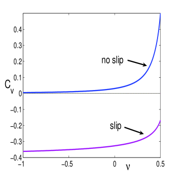
Figure 4: The virtual mass coefficient $C_{v}$ of the spherical inclusion plotted as a function of the Poisson’s ratio. The no-slip and slip curves correspond to $\chi=0$ and $\chi=1$ in Eq. (53), respectively.

5.4.2 Linear motion: Static displacement

Based on Eq. (5.4.1) we have

$${\mbox{\boldmath$\displaystyle\mathbf{U}$}}= \frac{3a}{2+\chi+\kappa^{-2}}\bigg{[}\frac{1}{r}{\mbox{\boldmath$\displaystyle\mathbf{I}$}}+\lim_{h\rightarrow 0}\,\nabla\nabla\frac{1}{h^{2}r}\bigg{(}\frac{e^{ih(r-a)}}{1-iha-\frac{1}{3}h^{2}a^{2}}$$

$$\qquad-\frac{e^{i\kappa^{-1}h(r-a)}}{1-i\kappa^{-1}ha-\frac{1}{3}\kappa^{-2}h^{2}a^{2}}\bigg{)}\bigg{]}$$

$$= \frac{3a}{2+\chi+\kappa^{-2}}\big{[}\frac{1}{r}{\mbox{\boldmath$\displaystyle\mathbf{I}$}}+\frac{1}{2}(\kappa^{-2}-1)\nabla\nabla\big{(}r+\frac{a^{2}}{3r}\big{)}\big{]}.$$ (54)

Evaluating the gradients and removing $\kappa$ in favor of $\nu$ gives

$${\mbox{\boldmath$\displaystyle\mathbf{U}$}}({\mbox{\boldmath$\displaystyle\mathbf{r}$}})= \frac{3a}{2r[5-6\nu+2\chi(1-\nu)]}\big{[}\big{(}3-4\nu+\frac{a^{2}}{3r^{2}}\big{)}{\mbox{\boldmath$\displaystyle\mathbf{I}$}}$$

$$+\big{(}1-\frac{a^{2}}{r^{2}}\big{)}\hat{\mbox{\boldmath$\displaystyle\mathbf{r}$}}\otimes\hat{\mbox{\boldmath$\displaystyle\mathbf{r}$}}\big{]},\quad\text{static \& immovable}.$$ (55)

This can be compared with Walpole’s Walpole (2005) result for the static perfectly bonded immovable spherical inclusion, Eq. (3.21) of Ref.  Walpole05. He considered the force tensor $\displaystyle\mathbf{\Phi}$, which as we have seen is equal to ${\mbox{\boldmath$\displaystyle\mathbf{U}$}}^{t}$ in the limit of a fixed and immovable rigid inclusion, i.e. $Z_{P}\rightarrow\infty$. But $\displaystyle\mathbf{U}$ is symmetric for the sphere, and therefore Eq. (5.4.2) represents both $\displaystyle\mathbf{U}$ and $\displaystyle\mathbf{\Phi}$. When $\chi=0$ this agrees with Walpole. The static result for $\chi=1$ appears to be new.

A more precise definition of the fixed inclusion limit is that $Z_{P}/Z\rightarrow\infty$. At the same time we are taking the static limit, so the simultaneous static and immovable limit is

$$\lim\limits_{\omega\rightarrow 0}\,\frac{a\mu}{\omega Z_{P}}=0.$$ (56)

5.4.3 Rotational motion: Virtual mass

In the limit of low frequency the rotational impedance ${\widetilde{Z}}$ of Eq. (32) for approximates as

$$\widetilde{Z}=\begin{cases}\frac{8\pi a^{3}\mu}{i\omega}+i\omega\frac{8}{3}\pi a^{5}\rho+\text{O}(\omega^{2}),&\text{no slip},\\ 0,&\text{slip},\end{cases}$$ (57)

where slip and no slip correspond to the limits $z_{I}=0$ and $z_{I}\rightarrow\infty$, respectively. The term $i\omega\frac{8}{3}\pi a^{5}\rho=2a^{2}Z_{M}$ can be identified as the virtual mass due to the rotating solid. The internal rotational impedance of a solid sphere is $\widetilde{Z}_{P}=\frac{2}{5}a^{2}{Z}_{P}$. Hence the virtual mass in rotation is five times the mass of solid matrix material in the volume of the sphere, in agreement with a similar result for Stokes flow Kendoush (2005).

5.4.4 Quasistatic plane wave force on an immovable particle

The forcing on the particle from plane wave incidence is the same, whether longitudinal or transverse waves are incident, in the quasistatic limit for a rigid immovable sphere. It may be checked that both (44) and (46) become

$${\mbox{\boldmath$\displaystyle\mathbf{F}$}}_{p}=\frac{12\pi a\mu}{2+\chi+\kappa^{-2}}\,{\mbox{\boldmath$\displaystyle\mathbf{u}$}}_{0}.$$ (58)

This apparently strange result may be reconciled with the physical nature of the limit: the matrix moves by the static displacement ${\mbox{\boldmath$\displaystyle\mathbf{u}$}}_{0}$, while the particle is stationary. It is therefore sensible that there is a net force on the particle, and that it is in the direction of ${\mbox{\boldmath$\displaystyle\mathbf{u}$}}_{0}$. This also explains the identical form of the limit for both types of wave incidence. The static limit is one of the unusual features of the the immovable sphere. For further discussion see Pao Pao and Mow (1973), who quite properly questions the physical validity of the rigid fixed assumption. Among its failings, as Pao notes, this configuration does not display Rayleigh scattering behavior at low frequencies.

5.4.5 Quasistatic plane wave moment on a fixed sphere

The moment on the rigid immovable spherical particle has a particularly simple form,

$${\mbox{\boldmath$\displaystyle\mathbf{M}$}}_{p}=\frac{-iha}{1-iha}4\pi a^{2}\mu\,\Omega\,e^{-iha}\,{\mbox{\boldmath$\displaystyle\mathbf{u}$}}_{0}\wedge{\mbox{\boldmath$\displaystyle\mathbf{n}$}},\quad\text{immovable}.$$ (59)

This is valid at all frequencies, but as $\omega\rightarrow 0$ it vanishes, unlike the force on the particle in the same limit.

5.5 Small inclusion limit

5.5.1 Linear motion

As $a\rightarrow 0$ we have $Z$, $Z_{L}$, $Z_{S}$, $Z_{T}$ = O$(a)$, while $Z_{M}$, $Z_{P}$ = o$(a)$. It may be easily verified that $\displaystyle\mathbf{U}$ and $\displaystyle\mathbf{\Phi}$ reduce in this limit to

$${\mbox{\boldmath$\displaystyle\mathbf{U}$}}({\mbox{\boldmath$\displaystyle\mathbf{r}$}})=i\omega Z\,{\mbox{\boldmath$\displaystyle\mathbf{G}$}}^{(0)}({\mbox{\boldmath$\displaystyle\mathbf{r}$}}),\qquad{\mbox{\boldmath$\displaystyle\mathbf{\Phi}$}}({\mbox{\boldmath$\displaystyle\mathbf{r}$}})=i\omega Z_{P}\,{\mbox{\boldmath$\displaystyle\mathbf{G}$}}^{(0)}({\mbox{\boldmath$\displaystyle\mathbf{r}$}}),$$ (60)

where ${\mbox{\boldmath$\displaystyle\mathbf{G}$}}^{(0)}$ is the free space Green’s tensor

$${\mbox{\boldmath$\displaystyle\mathbf{G}$}}^{(0)}({\mbox{\boldmath$\displaystyle\mathbf{r}$}})=\frac{1}{4\pi\mu}\bigg{[}\frac{e^{ihr}}{r}{\mbox{\boldmath$\displaystyle\mathbf{I}$}}+\nabla\nabla\bigg{(}\frac{1}{h^{2}r}\big{(}e^{ihr}-e^{ikr}\big{)}\bigg{)}\bigg{]}.$$ (61)

In hindsight, the form of $\displaystyle\mathbf{\Phi}$ is obvious based on the dynamic equilibrium of the inclusion : $i\omega Z_{P}{\mbox{\boldmath$\displaystyle\mathbf{u}$}}_{p}={\mbox{\boldmath$\displaystyle\mathbf{F}$}}_{p}$ with ${\mbox{\boldmath$\displaystyle\mathbf{u}$}}_{p}={\mbox{\boldmath$\displaystyle\mathbf{G}$}}^{(0)}{\mbox{\boldmath$\displaystyle\mathbf{F}$}}$, ${\mbox{\boldmath$\displaystyle\mathbf{F}$}}_{p}={\mbox{\boldmath$\displaystyle\mathbf{\Phi}$}}{\mbox{\boldmath$\displaystyle\mathbf{F}$}}$, and $\displaystyle\mathbf{U}$ then follows from (36).

5.5.2 Rotational motion

The rotational quantities $\displaystyle\mathbf{W}$ and $\displaystyle\mathbf{\Psi}$, on the other hand, become negligible in the small inclusion limit. This follows from the scaling ${\mbox{\boldmath$\displaystyle\mathbf{W}$}}=$O$(a)$ in Eq. (39).

5.6 Surface displacement and traction

5.6.1 Linear motion

The displacement tensor $\displaystyle\mathbf{U}$, which is defined in the exterior region, reduces to the following on the interface:

$${\mbox{\boldmath$\displaystyle\mathbf{U}$}}(a\hat{\mbox{\boldmath$\displaystyle\mathbf{r}$}})={\mbox{\boldmath$\displaystyle\mathbf{I}$}}+\big{(}\frac{Z_{S}-Z_{T}}{Z_{T}}\big{)}\big{(}\frac{Z+Z_{M}}{Z_{S}+Z_{M}}\big{)}\big{(}{\mbox{\boldmath$\displaystyle\mathbf{I}$}}-\hat{\mbox{\boldmath$\displaystyle\mathbf{r}$}}\otimes\hat{\mbox{\boldmath$\displaystyle\mathbf{r}$}}\big{)}.$$ (62)

This becomes the identity $\displaystyle\mathbf{I}$ under no-slip conditions, since then $Z_{S}-Z_{T}=0$. Alternatively, the interface conditions (28) can be written

$${\mbox{\boldmath$\displaystyle\mathbf{u}$}}={\mbox{\boldmath$\displaystyle\mathbf{u}$}}_{p}+(i\omega z_{I})^{-1}(\cdot\hat{\mbox{\boldmath$\displaystyle\mathbf{t}$}}\otimes\hat{\mbox{\boldmath$\displaystyle\mathbf{t}$}}){\mbox{\boldmath$\displaystyle\mathbf{\tau}$}},\qquad r=a.$$ (63)

The final term on the RHS vanishes as $z_{I}\rightarrow\infty$, which is the no-slip limit.

Substituting ${\mbox{\boldmath$\displaystyle\mathbf{u}$}}={\mbox{\boldmath$\displaystyle\mathbf{U}$}}(a\hat{\mbox{\boldmath$\displaystyle\mathbf{r}$}}){\mbox{\boldmath$\displaystyle\mathbf{u}$}}_{p}$ on $r=a$, in (63) provides an explicit expression for the interfacial shear traction in terms of the linear displacement ${\mbox{\boldmath$\displaystyle\mathbf{u}$}}_{p}$,

$${\mbox{\boldmath$\displaystyle\mathbf{\tau}$}}\cdot\hat{\mbox{\boldmath$\displaystyle\mathbf{t}$}}=i\omega z_{I}\,\big{(}\frac{Z_{S}-Z_{T}}{Z_{T}}\big{)}\big{(}\frac{Z+Z_{M}}{Z_{S}+Z_{M}}\big{)}\,{\mbox{\boldmath$\displaystyle\mathbf{u}$}}_{p}\cdot\hat{\mbox{\boldmath$\displaystyle\mathbf{t}$}}.$$ (64)

The shear traction vanishes under pure-slip conditions $(z_{I}=0)$, and for a bonded interface it becomes

$${\mbox{\boldmath$\displaystyle\mathbf{\tau}$}}\cdot\hat{\mbox{\boldmath$\displaystyle\mathbf{t}$}}=-i\omega{\mbox{\boldmath$\displaystyle\mathbf{u}$}}_{p}\cdot\hat{\mbox{\boldmath$\displaystyle\mathbf{t}$}}\,\frac{Z_{T}}{4\pi a^{2}}\,\big{(}\frac{Z+Z_{M}}{Z_{T}+Z_{M}}\big{)}.$$ (65)

5.6.2 Rotational motion

The displacement on $r=a$ is,

$${\mbox{\boldmath$\displaystyle\mathbf{W}$}}(a\hat{\mbox{\boldmath$\displaystyle\mathbf{r}$}})=-a\Omega\,\operatorname{axt}(\hat{\mbox{\boldmath$\displaystyle\mathbf{r}$}}),$$ (66)

where $\Omega$, given in (39), reduces to unity under no-slip conditions. Conversely, $\Omega=0$ for pure slip, indicating that the solid does not move even as the inclusion rotates.

In this case the traction is pure shear, and

$${\mbox{\boldmath$\displaystyle\mathbf{\tau}$}}=-i\omega\frac{3\widetilde{Z}}{8\pi a^{3}}\,{\mbox{\boldmath$\displaystyle\mathbf{\theta}$}}_{p}\wedge\hat{\mbox{\boldmath$\displaystyle\mathbf{r}$}},\qquad r=a.$$ (67)

This is non-zero except under pure slip conditions, when $\widetilde{Z}\rightarrow 0$, and there is no rotational interaction between the inclusion and the matrix.

5.7 Acoustic limit

5.7.1 General formulation

Finally, we discuss how the general elastodynamic formulation reduces when the matrix is an acoustic fluid. In this limit shear effects are ignorable and the medium is characterized by density $\rho$ and bulk modulus $K=\rho c^{2}$, where $c$ is the acoustic wave speed. Taking the displacement $\displaystyle\mathbf{u}$ and pressure $p$ as field variables, the momentum balance and constitutive law are, respectively,

$$\omega^{2}\rho{\mbox{\boldmath$\displaystyle\mathbf{u}$}}=\nabla p,\qquad p=-K\nabla\cdot{\mbox{\boldmath$\displaystyle\mathbf{u}$}}.$$ (68)

The acoustic wavenumber is $k=\omega/c$.

We introduce two vector functions ${\mbox{\boldmath$\displaystyle\mathbf{q}$}}({\mbox{\boldmath$\displaystyle\mathbf{r}$}})$ and ${\mbox{\boldmath$\displaystyle\mathbf{\phi}$}}({\mbox{\boldmath$\displaystyle\mathbf{s}$}})$ that are analogous to the tensors $\displaystyle\mathbf{U}$ and $\displaystyle\mathbf{\Phi}$. If the inclusion is moved back and forth with the displacement ${\mbox{\boldmath$\displaystyle\mathbf{u}$}}_{p}$ then the condition on the inclusion surface is that the normal velocity is continuous,

$${\mbox{\boldmath$\displaystyle\mathbf{u}$}}\cdot{\mbox{\boldmath$\displaystyle\mathbf{n}$}}={\mbox{\boldmath$\displaystyle\mathbf{u}$}}_{p}\cdot{\mbox{\boldmath$\displaystyle\mathbf{n}$}}\quad\text{on }\partial V_{p}.$$ (69)

The pressure at a point $\displaystyle\mathbf{r}$ away from inclusion is defined by $\displaystyle\mathbf{q}$ as

$$p({\mbox{\boldmath$\displaystyle\mathbf{r}$}})={\mbox{\boldmath$\displaystyle\mathbf{q}$}}({\mbox{\boldmath$\displaystyle\mathbf{r}$}})\cdot{\mbox{\boldmath$\displaystyle\mathbf{u}$}}_{p}\quad{\mbox{\boldmath$\displaystyle\mathbf{r}$}}\text{in }V.$$ (70)

Conversely, consider a voluminal source at $\displaystyle\mathbf{s}$:

$$\nabla^{2}p+k^{2}p=f\delta({\mbox{\boldmath$\displaystyle\mathbf{x}$}}-{\mbox{\boldmath$\displaystyle\mathbf{s}$}}).$$ (71)

The force on the inclusion is

$${\mbox{\boldmath$\displaystyle\mathbf{F}$}}_{p}=-\int\limits_{\partial V_{p}}\operatorname{d}s\,p\,{\mbox{\boldmath$\displaystyle\mathbf{n}$}}\equiv f\,{\mbox{\boldmath$\displaystyle\mathbf{\phi}$}}({\mbox{\boldmath$\displaystyle\mathbf{s}$}}),$$ (72)

which defines the vector function $\displaystyle\mathbf{\phi}$.

The connection between $\displaystyle\mathbf{q}$ and $\displaystyle\mathbf{\phi}$ is given by

Lemma 3

The acoustic displacement and force vectors are related by

$${\mbox{\boldmath$\displaystyle\mathbf{\phi}$}}({\mbox{\boldmath$\displaystyle\mathbf{s}$}})=(\rho\omega^{2})^{-1}\,{\mbox{\boldmath$\displaystyle\mathbf{Z}$}}_{P}({\mbox{\boldmath$\displaystyle\mathbf{Z}$}}+{\mbox{\boldmath$\displaystyle\mathbf{Z}$}}_{P})^{-1}{\mbox{\boldmath$\displaystyle\mathbf{q}$}}({\mbox{\boldmath$\displaystyle\mathbf{s}$}}).$$ (73)

This may be derived by application of reciprocity to the acoustic (Helmholtz) equation, in a manner similar to how we derived Lemma 2.

5.7.2 Spherical inclusion

Finally, we consider the example of the spherical inclusion. The vector $\displaystyle\mathbf{q}$ follows from the acoustic limit of the elastic result in (4.3.2),

$${\mbox{\boldmath$\displaystyle\mathbf{q}$}}({\mbox{\boldmath$\displaystyle\mathbf{r}$}})=aK\big{(}\frac{Z+Z_{M}}{Z_{A}+Z_{M}}\big{)}\,\nabla\frac{e^{ik(r-a)}}{r},\quad r\geq a,$$ (74)

where $Z_{A}$, analogous to the longitudinal impedance $Z_{L}$ in elasticity, is

$$Z_{A}=(i\omega)^{-1}4\pi aK\,(1-ika),$$ (75)

$Z_{M}$ is as before, and the sphere impedance $Z$ is now given by (30) with $Z_{S}=0$, which implies

$$\frac{1}{Z}=\frac{2}{Z_{M}}+\frac{3}{Z_{A}}.$$ (76)

6 Conclusion

Starting from the notion of an inclusion with the six degrees of freedom of a rigid body, we introduced displacement/rotation and force/moment tensors relating the motion of the inclusion to the displacement and force at arbitrary exterior points. These can be considered as generalized Green’s functions appropriate to the constrained nature of the inclusion. The general relations (7a) and (7b) between the displacement/rotation and force/moment tensors are one of the main contributions of the paper. These identities are extremely useful in providing a means by which one can consider the dynamic properties of particles embedded in a solid matrix.

Useful results have been obtained for the simplest but important configuration of a uniform spherical particle. The linear and rotational impedances, $Z$ and $\widetilde{Z}$, are given in Sections 4.2.1 and 4.2.2, respectively, the latter for the first time. Explicit expressions are given in Eqs. (36) - (40) for the displacement tensors $\displaystyle\mathbf{U}$ and $\displaystyle\mathbf{W}$ and for the force tensors $\displaystyle\mathbf{\Phi}$ and $\displaystyle\mathbf{\Psi}$. Perhaps the most practical new results are Eqs. (44), (46) and (48) which provide simple formulae for the force and moment on a particle under plane wave incidence. The associated displacement of the particle is given by Eq. (49). These concise expressions resemble Faxén relations that are frequently used in microhydrodynamics.

Equation (5.4.1) extends the quasistatic expansion of Norris Norris (2006) to include the virtual mass coefficient, which can be negative if slip occurs. The quasistatic form of $\displaystyle\mathbf{U}$, Eq. (5.4.2), which relates the displacement of the inclusion to particle displacement in the matrix, generalizes a recent formula of Walpole Walpole (2005). The quasistatic limit of the plane wave force on a sphere, Eq. (58), is reminiscent of Stokes drag law, but is proportional to the displacement vector of the incident plane wave. It also includes the possibility of slip relative to the matrix. However, the moment on a rigid sphere from plane wave incidence is proportional to the incident particle velocity, Eq. (59), and vanishes in the limit of zero frequency. Other limiting cases considered include the small inclusion limit, and the purely acoustic limit.

Taken together the results of paper offer a consistent means for analyzing wave-particle interaction in elasticity and viscoelasticity. Future applications will look at replacing the solid spherical particle with more complicated, and more interesting, internal structure. This amounts to considering more general forms of the internal impedances. The results developed here can also be used to develop simplified methods for scattering from particles. These issues will be examined in separate papers.

Appendix A Rotation of a sphere

The sphere $r\leq a$ undergoes oscillatory rotation ${\mbox{\boldmath$\displaystyle\mathbf{u}$}}_{P}={\mbox{\boldmath$\displaystyle\mathbf{\theta}$}}_{p}\wedge{\mbox{\boldmath$\displaystyle\mathbf{r}$}}$. Let $\displaystyle\mathbf{e}$ be the axis of rotation, so that ${\mbox{\boldmath$\displaystyle\mathbf{\theta}$}}_{p}=\theta_{p}{\mbox{\boldmath$\displaystyle\mathbf{e}$}}$, and consider the possible solution ${\mbox{\boldmath$\displaystyle\mathbf{u}$}}=\nabla\wedge{\mbox{\boldmath$\displaystyle\mathbf{e}$}}f$ in the matrix $r>a$. This satisfies the equations of motion

$${\mbox{\boldmath$\displaystyle\mathbf{u}$}}+k^{-2}\nabla\nabla\cdot{\mbox{\boldmath$\displaystyle\mathbf{u}$}}-h^{-2}\nabla\wedge\nabla\wedge{\mbox{\boldmath$\displaystyle\mathbf{u}$}}=0,$$ (77)

provided that $f$ is a solution of the reduced Helmholtz equation $\nabla^{2}f+h^{2}f=0$. The function $f$ must depend only on $r$ in order to match the prescribed rotation on $r=a$. Hence,

$${\mbox{\boldmath$\displaystyle\mathbf{u}$}}=\beta h_{1}(hr)\,{\mbox{\boldmath$\displaystyle\mathbf{e}$}}\wedge\hat{\mbox{\boldmath$\displaystyle\mathbf{r}$}},\quad r>a,$$ (78)

where $\hat{\mbox{\boldmath$\displaystyle\mathbf{r}$}}={\mbox{\boldmath$\displaystyle\mathbf{r}$}}/r$. The traction in an isotropic solid is Oestreicher (1951),

$${\mbox{\boldmath$\displaystyle\mathbf{\tau}$}}=\hat{\mbox{\boldmath$\displaystyle\mathbf{r}$}}\lambda\operatorname{div}{\mbox{\boldmath$\displaystyle\mathbf{u}$}}+\frac{\mu}{r}\operatorname{grad}{\mbox{\boldmath$\displaystyle\mathbf{r}$}}\cdot{\mbox{\boldmath$\displaystyle\mathbf{u}$}}+\mu\big{(}\frac{\partial}{\partial r}-\frac{1}{r}\big{)}{\mbox{\boldmath$\displaystyle\mathbf{u}$}},$$ (79)

from which we obtain

$${\mbox{\boldmath$\displaystyle\mathbf{\tau}$}}=\beta\mu h\big{[}h_{0}(ha)-\frac{3}{ha}h_{1}(ha)\big{]}{\mbox{\boldmath$\displaystyle\mathbf{e}$}}\wedge\hat{\mbox{\boldmath$\displaystyle\mathbf{r}$}}.$$ (80)

The boundary conditions (28) therefore reduce to a single equation for the parameter $\beta$ of Eq. (78),

$$\beta\mu h\big{[}h_{0}(ha)-\frac{3}{ha}h_{1}(ha)\big{]}=i\omega z_{I}\big{[}\beta h_{1}(ha)-a\theta_{p}\big{]}.$$ (81)

The moment ${\mbox{\boldmath$\displaystyle\mathbf{M}$}}_{p}=\int\operatorname{d}s{\mbox{\boldmath$\displaystyle\mathbf{r}$}}\wedge{\mbox{\boldmath$\displaystyle\mathbf{\tau}$}}$ is obtained from the identity

$$\int\limits_{r=a}\operatorname{d}s\,{\mbox{\boldmath$\displaystyle\mathbf{r}$}}\wedge({\mbox{\boldmath$\displaystyle\mathbf{e}$}}\wedge\hat{\mbox{\boldmath$\displaystyle\mathbf{r}$}})=\frac{8}{3}\pi a^{3}{\mbox{\boldmath$\displaystyle\mathbf{e}$}},$$ (82)

and the impedance then follows from the definition (6) as $\widetilde{\mbox{\boldmath$\displaystyle\mathbf{Z}$}}=\widetilde{Z}{\mbox{\boldmath$\displaystyle\mathbf{I}$}}$ where $\widetilde{Z}$ is given by (32).

Appendix B Displacement of a sphere

The solution to the radiation boundary value problem of the spherical inclusion undergoing linear displacement with boundary conditions defined by (28) has been solved by Oestreicher Oestreicher (1951) for the case of no slip and more recently, by Norris Norris (2006), with slip included. We follow the latter with some slight changes in notation. The solution is based on the following representation for the elastic field outside the sphere, $r\geq a$,

$${\mbox{\boldmath$\displaystyle\mathbf{u}$}}=-C_{1}\,{\mbox{\boldmath$\displaystyle\mathbf{u}$}}_{p}\cdot\nabla\nabla h_{0}(kr)+C_{2}\,{\mbox{\boldmath$\displaystyle\mathbf{u}$}}_{p}\cdot\big{(}\nabla\nabla-{\mbox{\boldmath$\displaystyle\mathbf{I}$}}\nabla^{2}\big{)}h_{0}(hr),$$ (83)

where $r=|{\mbox{\boldmath$\displaystyle\mathbf{r}$}}|$ is the spherical radius and $h_{0}$ is the spherical Hankel function of the first kind, $h_{0}(z)=(iz)^{-1}e^{iz}$.

In the notation of Ref.  norris2006b, $C_{1}=-A_{1}/k^{2}$ and $C_{2}=3B_{1}/h^{2}$. Also, with reference to Norris Norris (2006), the inclusion displacement is of magnitude $u_{0}$: ${\mbox{\boldmath$\displaystyle\mathbf{u}$}}_{p}=u_{0}\,\hat{\mbox{\boldmath$\displaystyle\mathbf{x}$}}$. Equations (15) and (19a) of Ref.  norris2006b combined with Eq. (29), give (noting that $Z_{m}$ of Ref.  norris2006b is now $Z_{M}$)

$$h_{2}(ka)A_{1} =\big{(}1+\frac{Z}{Z_{M}}\big{)}u_{0},$$ (84a)

$$6\frac{h_{1}(ha)}{ha}B_{1} =\frac{h_{1}(ka)}{ka}A_{1}-\frac{Z}{Z_{M}}u_{0}.$$ (84b)

Using $h_{1}(z)=-h_{0}^{\prime}(z)$ and $h_{2}=-h_{0}+3z^{-1}h_{1}$ implies the identities

$$\frac{h_{1}(ka)}{kah_{0}(ka)}=-\frac{Z_{L}}{3Z_{M}},\quad\frac{h_{2}(ka)}{h_{0}(ka)}=-\,\frac{Z_{L}+Z_{M}}{Z_{M}}.$$ (85)

Similar identities for arguments $ha$ instead of $ka$ have $Z_{T}$ instead of $Z_{L}$. Combining these results implies

$$C_{1} =\big{(}\frac{Z+Z_{M}}{Z_{L}+Z_{M}}\big{)}\,\frac{1}{k^{2}h_{0}(ka)},$$ (86a)

$$C_{2} =\big{(}\frac{Z+Z_{M}}{Z_{S}+Z_{M}}\big{)}\frac{Z_{S}}{Z_{T}}\,\frac{1}{h^{2}h_{0}(ha)}.$$ (86b)

The expression (4.3.2) for $\bf U$ then follows.

References

• Faxén (1927) H. Faxén. Simplified representation of the generalized Green’s equations for the constant motion of translation of a rigid body in a viscous fluid. Arkiv för Matematik, Astronomi och Fysik, 20(8):1–5, 1927.
• Happel and Brenner (1991) J. Happel and H. Brenner. Low Reynolds Number Hydrodynamics. Kluwer, Dordrecht, 1991.
• Kim and Karilla (1991) S. Kim and J. S. Karilla. Microhydrodynamics: Principles and Selected Applications. Butterworth-Heinemann, Boston, 1991.
• Pozrikidis (1997) C. Pozrikidis. Introduction to Theoretical and Computational Fluid Dynamics. Oxford University Press, New York, 1997.
• Phan-Thien and Kim (1994) N. Phan-Thien and S. Kim. Microstructures in Elastic Media: Principles and Computational Methods. Oxford University Press, New York, 1994.
• Norris (2006) A. N. Norris. Impedance of a sphere oscillating in an elastic medium with and without slip. J. Acoust. Soc. Am., 119(4):2062–2066, 2006. 10.1121/1.2171526.
• Oestreicher (1951) H. L. Oestreicher. Field and impedance of an oscillating sphere in a viscoelastic medium with an application to biophysics. J. Acoust. Soc. Am., 23:707– 714, 1951. 10.1121/1.1906828.
• Achenbach (2004) J. D. Achenbach. Reciprocity in Elastodynamics. Cambridge University Press, Cambridge, UK, 2004.
• Abramowitz and Stegun (1974) M. Abramowitz and I. Stegun. Handbook of Mathematical Functions with Formulas, Graphs, and Mathematical Tables. Dover, New York, 1974.
• Davis and Nagem (2006) A. M. Davis and R. J. Nagem. Curle’s equation and acoustic scattering by a sphere. J. Acoust. Soc. Am., 119(4):2018–2026, April 2006. 10.1121/1.2167611.
• Kendoush (2005) A. A. Kendoush. The virtual mass of a rotating sphere in fluids. J. Appl. Mech. ASME, 72(5):801–802, 2005. 10.1115/1.1989357.
• Walpole (2005) L. J. Walpole. The Green functions of an elastic medium surrounding a rigid spherical inclusion. Q. J. Mech. Appl. Math., 58(1):129–141, 2005. 10.1093/qjmamj/hbi001.
• Pao and Mow (1973) Y-H Pao and C-C Mow. Diffraction of Elastic Waves and Dynamic Stress Concentrations. Crane, Russak, New York, 1973.