DESY 07-103 ISSN 0418-9833
MPP-2007-96
July 2007

Electroweak corrections to $W$-boson hadroproduction at finite transverse momentum

Abstract

We calculate the full one-loop electroweak radiative corrections to the cross section of single $W$-boson inclusive hadroproduction at finite transverse momentum ($p_{T}$). This includes the $\mathcal{O}(\alpha)$ corrections to $W+j$ production, the $\mathcal{O}(\alpha_{s})$ corrections to $W+\gamma$ production, and the tree-level contribution from $W+j$ photoproduction with one direct or resolved photon in the initial state. We present the integrated cross section as a function of a minimum-$p_{T}$ cut as well as the $p_{T}$ distribution for the experimental conditions at the Fermilab Tevatron and the CERN LHC and estimate the theoretical uncertainties.

PACS: 12.15.Lk, 12.38.Bx, 13.85.Fb, 13.85.Qk

1 Introduction

The hadroproduction of single $W$ bosons via the Drell-Yan process in $p\overline{p}$ collisions at the CERN S$p\overline{p}$S led to the discovery of this particle in 1983 [1]. Nowadays, this process serves as a standard candle to calibrate and monitor the luminosity of hadronic collisions, since its cross section is rather sizeable and $W$ bosons are straightforward to identify experimentally thanks to their simple and distinct decay signature. The quality of the luminosity determination is thus limited by the precision to which this cross section is predicted theoretically. It is, therefore, mandatory to calculate higher-order radiative corrections. At present, they are known at next-to-leading order (NLO) [2] and next-to-next-to-leading order (NNLO) [3] in quantum chromodynamics (QCD) as well as at NLO [4] in the electroweak sector of the standard model (SM) of elementary particle physics.

In order for the $W$ boson to acquire finite transverse momentum ($p_{T}$), it must be produced in association with one or more other particles. To lowest order (LO) in QCD, the additional particle is a gluon ($g$), quark ($q$), or antiquark ($\overline{q}$), materialising as a hadron jet ($j$). The corresponding partonic subprocesses are of $\mathcal{O}(\alpha\alpha_{s})$. Their cross sections are presently known at NLO [5] and NNLO [6] in QCD, i.e. at $\mathcal{O}(\alpha\alpha_{s}^{2})$ and $\mathcal{O}(\alpha\alpha_{s}^{3})$, respectively. Very recently, also the one-loop electroweak corrections, at $\mathcal{O}(\alpha^{2}\alpha_{s})$, were considered [7]. This is also the topic of the present paper. However, as explained below, we actually study somewhat different cross section observables and arrange for our results to be manifestly infrared (IR) safe by avoiding kinematic cuts that destroy the inclusiveness of massless quanta. In fact, the situation is complicated by the circumstance that both photons and gluons can appear as bremsstrahlung.

The observable we thus wish to investigate is the differential cross section for the inclusive hadroproduction of single $W$ bosons with finite $p_{T}$ at $\mathcal{O}(\alpha^{2}\alpha_{s})$. Specifically, we concentrate on the $p_{T}$ distribution and the integrated cross section as a function of a minimum-$p_{T}$ cut, leaving the distributions in other observables, such as rapidity, for future work. At LO, the system $X$ recoiling against the $W$ boson is purely hadronic, while at $\mathcal{O}(\alpha^{2}\alpha_{s})$ it can include a photon ($\gamma$). We thus also have to consider $W+\gamma$ production, whose LO partonic cross sections are of $\mathcal{O}(\alpha^{2})$, because its NLO QCD correction contributes at the very order we are aiming at. In fact, the real radiative corrections to $W+j$ and $W+\gamma$ production receive contributions from a common set of $2\to 3$ partonic subprocesses. In the former (latter) case, IR singularities from the radiation of soft photons (gluons) cancel against similar contributions from virtual photons (gluons) by the Bloch-Nordsieck theorem [8]. Similarly, the IR singularities from collinear final-state radiation (FSR) cancel against similar contributions from the virtual corrections by the Kinoshita-Lee-Nauenberg theorem [9]. The residual IR singularities from collinear initial-state radiation (ISR) are factorised and absorbed at $\mathcal{O}(\alpha)$ ($\mathcal{O}(\alpha_{s})$) into the parton distribution functions (PDFs). This procedure leads to manifestly IR-safe cross section observables and translates into unique and simple event selection criteria on the experimental side.

By contrast, the notion of electroweak NLO corrections to $W+j$ production comprises a conceptual problem. In fact, in the treatment of final-state collinear singularities caused by the parallel emission of a photon from an outgoing (anti)quark line, one is led to introduce a cut in an appropriate separation variable. Within the collinear phase space region thus defined, the (anti)quark-photon system is effectively treated as one particle whose momentum is identified with that of $j$ and thus subject to an acceptance cut in transverse momentum, $p_{T}(j)>p_{T}^{\mathrm{min}}(j)$, to ensure the experimental observation of $j$. This includes phase space configurations where the photon essentially carries all the momentum, while the (anti)quark can, in principle, be arbitrarily soft. This will not generate any soft IR singularities. However, since (anti)quark and gluon jets can, in general, not be distinguished experimentally on an event-by-event basis, the same recombination procedure needs to be applied to a gluon-photon system in the final state as well. This time, a soft gluon will inevitably produce an IR singularity, which can only be canceled by the NLO QCD corrections to $W+\gamma$ production, so that one falls back to the symmetric procedure outlined in the preceding paragraph. Formally, this soft-gluon singularity can be avoided by applying the $p_{T}^{\mathrm{min}}(j)$ cut just to the transverse momentum of the gluon, even if it is accompanied by a collinear photon. However, such a prescription is purely academic and quite unsuitable for experimental implementation because (anti)quark and gluon jets are treated on different footings.

By crossing external lines, the LO partonic subprocesses of $W+\gamma$ hadroproduction can be converted to those of $W+j$ photoproduction with one incoming photon participating directly in the hard scattering (direct photoproduction). The emission of photons off the proton can happen either elastically or inelastically, i.e. the proton stays intact or is destroyed, respectively. In both cases, an appropriate PDF can be evaluated in the Weizsäcker-Williams approximation [10, 11, 12]. Since they are of $\mathcal{O}(\alpha)$, these direct photoproduction contributions are of $\mathcal{O}(\alpha^{3})$. Incoming photons can participate in the hard scattering also through their quark and gluon content, leading to resolved photoproduction. The contributions from direct and resolved photoproduction are formally of the same order in the perturbative expansion. This may be understood by observing that the PDFs of the photon have a leading behaviour proportional to $\alpha\ln(M^{2}/\Lambda_{\mathrm{QCD}}^{2})\propto\alpha/\alpha_{s}$, where $M$ is the factorisation scale and $\Lambda_{\mathrm{QCD}}$ is the asymptotic scale parameter of QCD. Although photoproduction contributions are parametrically suppressed by a factor of $\alpha/\alpha_{s}$ relative to the $\mathcal{O}(\alpha^{2}\alpha_{s})$ corrections discussed above, we shall include them in our analysis because they turn out to be quite sizeable in an extensive region of phase space.

This paper is organised as follows. In Section 2, we list the partonic cross sections at LO and explain how to evaluate the hadronic cross section from them. In Section 3, we discuss in detail the structure of the NLO corrections. In Section 4, we present our numerical results for $p\overline{p}$ collisions with centre-of-mass (c.m.) energy $\sqrt{S}=1.96$ TeV at the Fermilab Tevatron and $pp$ collisions with $\sqrt{S}=14$ TeV at the CERN Large Hadron Collider (LHC).

2 Conventions and LO results

We consider the hadronic process

$$A(p_{A})+B(p_{B})\to W(p)+X,$$ (2.1)

where the four-momentum assignments are indicated in parentheses. We work in the collinear parton model of QCD [13] with $n_{f}=5$ massless quark flavours $q=u,d,s,c,b$, neglect the masses of the incoming hadrons, $A$ and $B$, and impose the acceptance cut $p_{T}>p_{T}^{\mathrm{cut}}$ on the transverse momentum $p_{T}$ of the $W$ boson. (We assign masses to the partons $\gamma,g,q,\overline{q}$ only to regulate soft and collinear IR singularities in intermediate steps of our calculation.)

Specifically, denoting $u_{1}=u$, $u_{2}=c$, $d_{1}=d$, $d_{2}=s$, and $d_{3}=b$, the relevant partonic subprocesses include

$$u_{i}+\overline{d}_{j} \to W^{+}+g,$$ (2.2)

$$u_{i}+g \to W^{+}+d_{j},$$ (2.3)

$$\overline{d}_{j}+g \to W^{+}+\overline{u}_{i},$$ (2.4)

at $\mathcal{O}(\alpha\alpha_{s})$,

$$u_{i}+\overline{d}_{j} \to W^{+}+\gamma,$$ (2.5)

$$u_{i}+\gamma \to W^{+}+d_{j},$$ (2.6)

$$\overline{d}_{j}+\gamma \to W^{+}+\overline{u}_{i},$$ (2.7)

at $\mathcal{O}(\alpha^{2})$, and

$$u_{i}+\overline{d}_{j} \to W^{+}+g+\gamma,$$ (2.8)

$$u_{i}+g \to W^{+}+d_{j}+\gamma,$$ (2.9)

$$\overline{d}_{j}+g \to W^{+}+\overline{u}_{i}+\gamma,$$ (2.10)

at $\mathcal{O}(\alpha^{2}\alpha_{s})$. The partonic subprocesses involving a $W^{-}$ boson emerge through charge conjugation. Processes (2.2)–(2.5) must be treated also at one loop, $\mathcal{O}(\alpha^{2}\alpha_{s})$. Processes (2.6) and (2.7) contribute to direct photoproduction and processes (2.2)–(2.4) to resolved photoproduction. Since photon emission off protons happens at $\mathcal{O}(\alpha)$, it is sufficient to deal with photoproduction at tree level. In summary, we calculate the cross section of process (2.1) at NLO as the sum

$$\sigma^{AB\to WX}=\sigma_{0}^{Wj}+\sigma_{0}^{W\gamma}+\sigma_{\mathcal{O}(\alpha)}^{Wj}+\sigma_{\mathcal{O}(\alpha_{s})}^{W\gamma}+\sigma_{0}^{Wj\gamma}+\sigma_{\gamma}^{Wj},$$ (2.11)

where $\sigma_{0}^{Wj}$ and $\sigma_{\mathcal{O}(\alpha)}^{Wj}$ are due to processes (2.2)–(2.4) at tree level and one loop, $\sigma_{0}^{W\gamma}$ and $\sigma_{\mathcal{O}(\alpha_{s})}^{W\gamma}$ are due to process (2.5) at tree level and one loop, $\sigma_{0}^{Wj\gamma}$ is due to processes (2.8)–(2.10) at tree level, and $\sigma_{\gamma}^{Wj}$ is due to processes (2.6) and (2.7) via direct photoproduction and due to processes (2.2)–(2.4) via resolved photoproduction, both at tree-level.

The minimum-$p_{T}$ cut is necessary to stay away from the regions of phase space that are sensitive to the collinear IR singularities due to the $q\to\gamma/g+q^{\ast}$, $\overline{q}\to\gamma/g+\overline{q}^{\ast}$, $\gamma/g\to q+\overline{q}^{\ast}$, and $\gamma/g\to\overline{q}+q^{\ast}$ splittings, which are present already at LO. Here, an asterisk marks a virtual parton. The cross section $\sigma^{AB\to WX}$ of the hadronic process (2.1) is related to the cross sections $\hat{\sigma}^{ab\to Wc(d)}$ of the partonic subprocesses,

$$a(p_{a})+b(p_{b})\to W(p)+c(p_{c})(+d(p_{d})),$$ (2.12)

where $a,b,c,d=\gamma,g,q,\overline{q}$ and $p_{a}=x_{a}p_{A}$, $p_{b}=x_{b}p_{B}$ with scaling parameters $x_{a}$, $x_{b}$, as the incoherent sum

$$\sigma^{AB\to WX}(S,p_{T}>p_{T}^{\mathrm{cut}})=\sum_{a,b,c(,d)}\int_{\tau_{0}}^{1}\mathrm{d}\tau\,\mathcal{L}_{ab}^{AB}(\tau)\hat{\sigma}^{ab\to Wc(d)}(s,p_{T}>p_{T}^{\mathrm{cut}}),$$ (2.13)

where $S=(p_{A}+p_{B})^{2}$ and $s=(p_{a}+p_{b})^{2}=\tau S$ are the hadronic and partonic c.m. energies, respectively, $\tau=x_{a}x_{b}$, and

$$\mathcal{L}_{ab}^{AB}(\tau)=\int_{\tau}^{1}\frac{\mathrm{d}x_{a}}{x_{a}}f_{a/A}(x_{a},M^{2})f_{b/B}\left(\frac{\tau}{x_{a}},M^{2}\right)$$ (2.14)

is the parton luminosity defined in terms of the PDFs $f_{a/A}(x_{a},M^{2})$, $f_{b/B}(x_{b},M^{2})$. Here, $M$ denotes the factorisation mass scale. Introducing the short-hand notation $w=M_{W}^{2}$, we have

$$\tau_{0}=\frac{\left(p_{T}^{\mathrm{cut}}+\sqrt{w+(p_{T}^{\mathrm{cut}})^{2}}\right)^{2}}{S}.$$ (2.15)

In order to obtain $\hat{\sigma}^{ab\to Wc(d)}$, we have to evaluate the transition matrix elements $\mathcal{T}^{ab\to Wc(d)}$ of processes (2.12), square them, average them over the initial-state spins and colours, and sum them over the final-state ones, which leads to $\overline{|\mathcal{T}^{ab\to Wc(d)}|^{2}}$. To the order of our calculation, $\mathcal{T}^{ab\to Wcd}$ is calculated at tree level, while $\mathcal{T}^{ab\to Wc}$ may receive also one-loop contributions, $\mathcal{T}^{ab\to Wc}=\mathcal{T}_{0}^{ab\to Wc}+\mathcal{T}_{1}^{ab\to Wc}$, so that

$$\overline{\left|\mathcal{T}^{ab\to Wc}\right|^{2}}=\overline{\left|\mathcal{T}_{0}^{ab\to Wc}\right|^{2}}+2\mathop{\mathrm{Re}}\nolimits\overline{\left[\left(\mathcal{T}_{0}^{ab\to Wc}\right)^{*}\mathcal{T}_{1}^{ab\to Wc}\right]}.$$ (2.16)

Then we have to integrate over the partonic phase spaces imposing the minimum-$p_{T}$ cut. In the following two subsections, we describe how this can be conveniently done for the two- and three-particle final states, respectively.

Since we are dealing with charged-current interactions of quarks, $u_{i}$ and $d_{j}$, the Cabibbo-Kobayashi-Maskawa quark mixing matrix $V_{ij}$ appears. At tree level, the cross sections of processes (2.2)–(2.10) contain the overall factor $|V_{ij}|^{2}$, and a part of the one-loop corrections is proportional to $V_{ij}^{*}V_{ij^{\prime}}V_{i^{\prime}j^{\prime}}^{*}V_{i^{\prime}j}$, where $u_{i^{\prime}}$ and $d_{j^{\prime}}$ are virtual quarks. Since we neglect all down-quark masses, we can sum over the indices of the virtual and outgoing down quarks to trigger the unitarity relation $\sum_{j=1}^{3}V_{ij}V_{i^{\prime}j}^{*}=\delta_{ii^{\prime}}$. In the case of incoming down quarks, we can absorb the residual appearances of $|V_{ij}|^{2}$ into a redefinition of their PDFs, as [7]

$$\tilde{f}_{d_{i}/A}(x,M^{2})=\sum_{j=1}^{3}\left|V_{ij}\right|^{2}f_{d_{j}/A}(x,M^{2}),$$ (2.17)

and similarly for down antiquarks. Therefore, it is sufficient to calculate the partonic cross sections for the flavour-diagonal case, with $V_{ij}=\delta_{ij}$.

2.1 Two-particle final state

If parton $d$ is absent in process (2.12), we supplement $s$ by two more Mandelstam variables, $t=(p_{a}-p)^{2}$ and $u=(p_{b}-p)^{2}$. Four-momentum conservation implies that $s+t+u=w$, and we have $p_{T}^{2}=tu/s$. The partonic cross section entering Eq. (2.13) is evaluated as

$$\hat{\sigma}^{ab\to Wc}(s,p_{T}>p_{T}^{\mathrm{cut}})=\int_{p_{T}^{\mathrm{cut}}}^{p_{T}^{\mathrm{max}}}\mathrm{d}p_{T}\frac{\mathrm{d}\hat{\sigma}^{ab\to Wc}}{\mathrm{d}p_{T}},$$ (2.18)

where $p_{T}^{\mathrm{max}}=(s-w)/(2\sqrt{s})$ and

$$\frac{\mathrm{d}\hat{\sigma}^{ab\to Wc}}{\mathrm{d}p_{T}}=\frac{p_{T}}{8\pi s\sqrt{(s-w)^{2}-4sp_{T}^{2}}}\overline{\left|\mathcal{T}^{ab\to Wc}\right|^{2}}+(t\leftrightarrow u).$$ (2.19)

For the reader’s convenience, we list the differential cross sections of processes (2.2)–(2.7), in the conventional form

$$\frac{\mathrm{d}\hat{\sigma}^{ab\to Wc}}{\mathrm{d}t}=\frac{1}{16\pi s^{2}}\overline{\left|\mathcal{T}^{ab\to Wc}\right|^{2}},$$ (2.20)

at LO. The Feynman diagrams contributing to processes (2.2) and (2.5) are displayed in Figs. 1 (a) and (b), respectively. We have

$$\frac{\mathrm{d}\hat{\sigma}^{u\overline{d}\to W^{+}g}}{\mathrm{d}t} = \frac{2\pi\alpha\alpha_{s}}{9s_{w}^{2}}\,\frac{s^{2}+w^{2}-2tu}{s^{2}tu},$$

$$\frac{\mathrm{d}\hat{\sigma}^{u\overline{d}\to W^{+}\gamma}}{\mathrm{d}t} = \frac{\alpha}{12\alpha_{s}}\left(1+\frac{3t}{s-w}\right)^{2}\frac{\mathrm{d}\hat{\sigma}^{u\overline{d}\to W^{+}g}}{\mathrm{d}t},$$ (2.21)

where $s_{w}=\sin\theta_{w}$ is the sine of the weak-mixing angle. Since the $W$-boson mass sets the renormalisation scale of the couplings, it is natural to adopt the definition of Sommerfeld’s fine-structure constant $\alpha$ in terms of Fermi’s constant $G_{F}$,

$$\alpha=\frac{\sqrt{2}}{\pi}G_{F}s_{w}^{2}w.$$ (2.22)

The implementation of this renormalisation scheme at one loop is explained in Section 3.1. The cross sections of processes (2.3), (2.4), (2.6), and (2.7) may be obtained from Eq. (2.21) by exploiting crossing symmetries, as

$$s^{2}\frac{\mathrm{d}\hat{\sigma}^{ug\to W^{+}d}}{\mathrm{d}t} = -\frac{3}{8}\left[s^{2}\frac{\mathrm{d}\hat{\sigma}^{u\overline{d}\to W^{+}g}}{\mathrm{d}t}\right]_{s\leftrightarrow u},$$

$$s^{2}\frac{\mathrm{d}\hat{\sigma}^{\overline{d}g\to W^{+}\overline{u}}}{\mathrm{d}t} = \left[s^{2}\frac{\mathrm{d}\hat{\sigma}^{ug\to W^{+}d}}{\mathrm{d}t}\right]_{s\leftrightarrow t},$$

$$s^{2}\frac{\mathrm{d}\hat{\sigma}^{u\gamma\to W^{+}d}}{\mathrm{d}t} = -3\left[s^{2}\frac{\mathrm{d}\hat{\sigma}^{u\overline{d}\to W^{+}\gamma}}{\mathrm{d}t}\right]_{s\leftrightarrow u},$$

$$s^{2}\frac{\mathrm{d}\hat{\sigma}^{\overline{d}\gamma\to W^{+}\overline{u}}}{\mathrm{d}t} = \left[s^{2}\frac{\mathrm{d}\hat{\sigma}^{u\gamma\to W^{+}d}}{\mathrm{d}t}\right]_{s\leftrightarrow t}.$$ (2.23)

2.1.1 Three-particle final states

If parton $d$ is present in process (2.12), then the partonic cross section entering Eq. (2.13) may be obtained through a four-fold phase-space integration along the lines of Ref. [14]. We work in the partonic c.m. frame and choose our coordinate system so that $\vec{p_{a}}$ points along the $z$ direction and $\vec{p_{d}}$ lies in the $x$-$y$ plane. We denote the polar angle of $\vec{p_{d}}$ by $\vartheta$ and the azimuthal angle of $\vec{p_{c}}$ by $\varphi$. As the first three independent variables, we select $p_{d}^{0}$, $\vartheta$, and $\varphi$, which take the values

$$0<p_{d}^{0}<\frac{s-w}{2\sqrt{s}},\qquad 0<\vartheta<\pi,\qquad 0<\varphi<2\pi.$$ (2.24)

In the case of process (2.8), which contains two massless gauge bosons in the final state, it is convenient to take the fourth variable to be $p_{c}^{0}$, with values

$$\frac{1}{2}\left(\sqrt{s}-2p_{d}^{0}-\frac{w}{\sqrt{s}}\right)<p_{c}^{0}<\frac{1}{2}\left(\sqrt{s}-\frac{w}{\sqrt{s}-2p_{d}^{0}}\right).$$ (2.25)

We then have

$$\left.\frac{\mathrm{d}^{4}\hat{\sigma}^{u\overline{d}\to W^{+}g\gamma}}{\mathrm{d}p_{c}^{0}\mathrm{d}p_{d}^{0}\mathrm{d}\cos\vartheta\mathrm{d}\varphi}\right|_{p_{T}>p_{T}^{\mathrm{cut}}}=\frac{1}{8(2\pi)^{4}}\overline{\left|\mathcal{T}^{u\overline{d}\to W^{+}g\gamma}\right|^{2}}\theta\left(p_{T}-p_{T}^{\mathrm{cut}}\right).$$ (2.26)

On the other hand, in the case of processes (2.9) and (2.10), which only contain one massless gauge boson in the final state, it is more useful to choose the fourth variable to be the angle $\psi$ enclosed between $\vec{p}_{c}$ and $\vec{p}_{d}$, with values

$$0<\psi<\pi.$$ (2.27)

We then have

$$\left.\frac{\mathrm{d}^{4}\hat{\sigma}^{ug\to W^{+}d\gamma}}{\mathrm{d}p_{d}^{0}\mathrm{d}\cos\vartheta\mathrm{d}\varphi\mathrm{d}\psi}\right|_{p_{T}>p_{T}^{\mathrm{cut}}}=\frac{p_{d}^{0}\left[\sqrt{s}\left(\sqrt{s}-2p_{d}^{0}\right)-w\right]}{16(2\pi)^{4}\left[\sqrt{s}-2p_{d}^{0}\sin^{2}(\psi/2)\right]^{2}}\overline{\left|\mathcal{T}^{ug\to W^{+}d\gamma}\right|^{2}}\theta\left(p_{T}-p_{T}^{\mathrm{cut}}\right),$$ (2.28)

and similarly for process (2.10). In order to implement the minimum-$p_{T}$ cut, $p_{T}$ needs to be expressed in terms of the integration variables, which is conveniently done with the help of Eqs. (5.40) and (5.42) of Ref. [14] and starting from

$$p_{T}=\sqrt{\left(p_{c}^{1}+p_{d}^{1}\right)^{2}+\left(p_{c}^{2}+p_{d}^{2}\right)^{2}}.$$ (2.29)

3 NLO results

We now describe the calculation of the NLO contributions $\sigma_{\mathcal{O}(\alpha)}^{Wj}$, $\sigma_{\mathcal{O}(\alpha_{s})}^{W\gamma}$, and $\sigma_{0}^{Wj\gamma}$ of Eq. (2.11) in some detail.

We employ the following tools. We generate the relevant Feynman diagrams using the symbolic program package FeynArts [15], carry out the spin and colour sums using the program package FormCalc [16], and perform the Passarino-Veltman reduction of the tensor one-loop integrals [17] using the program package FeynCalc [18]. Subsequently, we implement the analytical results in a Fortran program. We evaluate the standard scalar one-loop integrals contained in the purely weak corrections using the program package LoopTools [19], which incorporates the program library FF [20]. The numerical integrations are performed using the program package Cuba [21], which provides several different integration routines and is, therefore, also well suited for cross checks.

3.1 Virtual electroweak corrections to $W+j$ production

The virtual electroweak corrections of $\mathcal{O}(\alpha)$ to processes (2.2)–(2.4) arise from self-energy, triangle, box, and counterterm diagrams. They are shown for process (2.2) in Figs. 2–5, respectively.

Evaluating the transition matrix element $\mathcal{T}_{\mathcal{O}(\alpha)}^{Wj}$ from these loop diagrams, we encounter both ultraviolet (UV) and IR singularities, which need to be regularised and removed. As usual, we use dimensional regularisation, with $D=4-2\epsilon$ space-time dimensions and ’t Hooft mass scale $\mu$, to extract the UV singularities as single poles in $\epsilon$. These are removed by renormalising the parameters and wave functions of the LO transition matrix element $\mathcal{T}_{0}^{Wj}$, which leads to the counterterm contribution (see Fig. 5),

$$\mathcal{T}_{\mathrm{CT}}^{Wj}=\mathcal{T}_{0}^{Wj}\delta_{\mathrm{CT}}^{Wj}.$$ (3.1)

Owing to the renormalisability of the SM, the UV singularities in $\mathcal{T}_{\mathcal{O}(\alpha)}^{Wj}$ cancel, and the physical limit $\epsilon\to 0$ can be reached smoothly.

The electroweak on-shell renormalisation scheme uses the fine-structure constant $\alpha$ defined in the Thomson limit and the physical particle masses as basic parameters. In order to avoid the appearance of large logarithms induced by the running of $\alpha$ to the electroweak scale $M_{W}$ in $\mathcal{T}_{\mathcal{O}(\alpha)}^{Wj}$, it is useful to replace $\alpha$ by $G_{F}$ in the set of basic parameters, by substituting

$$G_{F}=\frac{\pi\alpha}{\sqrt{2}s_{w}^{2}w}\,\frac{1}{1-\Delta r},$$ (3.2)

where $\Delta r$ [22] contains those radiative corrections to the muon lifetime which the SM introduces on top of those derived in the QED-improved Fermi model. In the electroweak on-shell scheme thus modified, we have

$$\delta_{\mathrm{CT}}^{Wj}=\delta Z_{e}-\frac{\delta s_{w}}{s_{w}}+\frac{1}{2}\left(\delta Z_{u\overline{u}}^{\mathrm{L}}+\delta Z_{d\overline{d}}^{\mathrm{L}}+\delta Z_{W}-\Delta r\right),$$ (3.3)

where the renormalisation constants read [23]

$$\frac{\delta s_{w}}{s_{w}} = -\frac{1}{2}\,\frac{c_{w}^{2}}{s_{w}^{2}}\,\mathop{\mathrm{Re}}\nolimits\left[\frac{\Sigma_{WW}^{\mathrm{T}}(M_{W}^{2})}{M_{W}^{2}}-\frac{\Sigma_{ZZ}^{\mathrm{T}}(M_{Z}^{2})}{M_{Z}^{2}}\right],$$

$$\delta Z_{e} = \frac{1}{2}\,\left.\frac{\partial\Sigma_{AA}^{\mathrm{T}}(q^{2})}{\partial q^{2}}\right|_{q^{2}=0}-\frac{s_{w}}{c_{w}}\,\frac{\Sigma_{AZ}^{\mathrm{T}}(0)}{M_{Z}^{2}},$$

$$\delta Z_{W} = -\mathop{\mathrm{Re}}\nolimits\left.\frac{\partial\Sigma_{WW}^{\mathrm{T}}(q^{2})}{\partial q^{2}}\right|_{q^{2}=M_{W}^{2}},$$

$$\delta Z_{q\overline{q}}^{\mathrm{L}} = -\mathop{\mathrm{Re}}\nolimits\Sigma_{q\overline{q}}^{\mathrm{L}}(m_{q}^{2})-m_{q}^{2}\left.\frac{\partial}{\partial q^{2}}\mathop{\mathrm{Re}}\nolimits\left[\Sigma_{q\overline{q}}^{\mathrm{L}}(q^{2})+\Sigma_{q\overline{q}}^{\mathrm{R}}(q^{2})+2\Sigma_{q\overline{q}}^{\mathrm{S}}(q^{2})\right]\right|_{q^{2}=m_{q}^{2}}.$$ (3.4)

Here, $\Sigma_{WW}^{\mathrm{T}}$, $\Sigma_{ZZ}^{\mathrm{T}}$, $\Sigma_{AA}^{\mathrm{T}}$, and $\Sigma_{AZ}^{\mathrm{T}}$ are the transverse parts of the respective electroweak gauge-boson self-energies and mixing amplitudes, $\Sigma_{q\overline{q}}^{\mathrm{L}}$, $\Sigma_{q\overline{q}}^{\mathrm{R}}$, and $\Sigma_{q\overline{q}}^{\mathrm{S}}$ are the left-handed, right-handed, and scalar parts of the quark self-energy, and $c_{w}^{2}=1-s_{w}^{2}$.

The IR singularities can be of soft or collinear type. The loop diagrams involving virtual photons interchanged between external lines are plagued by soft IR singularities. Owing to the Bloch-Nordsieck theorem [8], they cancel against similar singularities arising from the real emission of soft photons, to be discussed in Section 3.3. The loop diagrams involving external quark or antiquark lines that split into virtual photons and quarks generate collinear IR singularities. Such singularities also arise from the real emission of collinear photons off external quark or antiquark lines, as will be explained in Section 3.3. Thanks to the Kinoshita-Lee-Nauenberg theorem [9], collinear IR singularities from FSR are completely canceled in the sum of real and virtual corrections provided that the final state is treated inclusively enough. On the other hand, collinear IR singularities from ISR survive and have to be absorbed into the quark and antiquark PDFs. For consistency, the splitting functions in the evolution equations of the PDFs then need to be complemented by their $\mathcal{O}(\alpha)$ terms. IR singularities also arise from the wave-function renormalisations in Eq. (3.4). We choose to regularise the IR singularities by assigning infinitesimal masses, $\lambda$, $m_{u}$, and $m_{d}$, to the photon, the light up-type quarks, and the down-type quarks, respectively. This is convenient because the standard scalar one-loop integrals $C_{0}$ and $D_{0}$ that emerge after the tensor reduction [17] are well established for this regularisation prescription [24]. Although the purely weak loop corrections are altogether devoid of IR singularities, terms logarithmic in $m_{u}$ and $m_{d}$ are generated by the tensor reduction. However, these artificial IR singularities cancel among themselves.

We emphasise that, in the treatment of both the virtual and real corrections, terms depending on $\lambda$, $m_{u}$, and $m_{d}$ are extracted analytically and their cancellation is established manifestly, so that the expressions used for the numerical analysis do not contain these IR regulators.

3.2 Virtual QCD corrections to $W+\gamma$ production

The virtual QCD corrections of $\mathcal{O}(\alpha_{s})$ to process (2.5) arise from the self-energy, triangle, and box diagrams shown in Fig. 6 and the counterterm contribution,

$$\mathcal{T}_{\mathrm{CT}}^{W\gamma}=\mathcal{T}_{0}^{W\gamma}\delta_{\mathrm{CT}}^{W\gamma}.$$ (3.5)

The latter only receives contributions from the gluon-induced wave-function renormalisation of the external quark lines,

$$\delta_{\mathrm{CT}}^{W\gamma}=\frac{1}{2}\left(\delta Z_{u\overline{u}}^{g}+\delta Z_{d\overline{d}}^{g}\right),$$ (3.6)

where

$$\delta Z_{q\overline{q}}^{g}=-\Sigma_{q\overline{q}}^{g,\mathrm{V}}(m_{q}^{2})-2m_{q}^{2}\left.\frac{\partial}{\partial q^{2}}\left[\Sigma_{q\overline{q}}^{g,\mathrm{V}}(q^{2})+\Sigma_{q\overline{q}}^{g,\mathrm{S}}(q^{2})\right]\right|_{q^{2}=m_{q}^{2}}.$$ (3.7)

Because parity is conserved within QCD, the quark self-energy has just one vector part $\Sigma_{q\overline{q}}^{g,\mathrm{V}}=\Sigma_{q\overline{q}}^{g,\mathrm{L}}=\Sigma_{q\overline{q}}^{g,\mathrm{R}}$. Up to terms that vanish in the limit $m_{q}\to 0$, we have

$$\delta Z_{q\overline{q}}^{g}=-\frac{\alpha_{s}C_{F}}{4\pi}\left[\frac{1}{\epsilon}-\gamma_{E}+\ln(4\pi)-\ln\frac{m_{q}^{2}}{\mu^{2}}-2\ln\frac{m_{q}^{2}}{\lambda^{2}}+4\right]+\mathcal{O}(\epsilon),$$ (3.8)

where $C_{F}=(N_{c}^{2}-1)/(2N_{c})=4/3$ for $N_{c}=3$ quark colours, $\gamma_{E}$ is the Euler-Mascheroni constant, and $\lambda$ now represents an infinitesimal gluon mass.

3.3 Real corrections due to $W+j+\gamma$ production

The tree-level diagrams for process (2.8) are shown in Fig. 7. They contribute at the same time to the electromagnetic bremsstrahlung in process (2.2) and to the QCD bremsstrahlung in process (2.5), which complicates the treatment of the electroweak corrections to $W+j$ associated production, as explained in the Introduction. The diagrams contributing to the electromagnetic bremsstrahlung in processes (2.3) and (2.4) emerge from Fig. 7 by crossing the gluon with the $u$ and $\overline{d}$ quarks, respectively.

When the cross sections of processes (2.8)–(2.10) are integrated over their three-particle phase spaces, one encounters IR singularities of both soft and collinear types. The former stem from the emission of soft photons and gluons and cancel against similar contributions from the virtual corrections owing to the Block-Nordsieck theorem [8], as explained in Section 3.1. The latter arise when a massless gauge boson is collinearly emitted from an external massless fermion line or when a massless gauge boson splits into two collinear massless fermions. Specifically, in process (2.8), the photon or the gluon can be emitted collinearly from the incoming $u_{i}$ and $\overline{d}_{j}$ quarks; in process (2.9), the photon can be emitted collinearly from the incoming $u_{i}$ quark or the outgoing $d_{j}$ quark, and the gluon can split into a collinear $d_{j}\overline{d}_{j}$ quark pair; and in process (2.10), the photon can be emitted collinearly from the incoming $\overline{d}_{j}$ quark or the outgoing $\overline{u}_{i}$ quark, and the gluon can split into a collinear $u_{i}\overline{u}_{i}$ quark pair. As already mentioned in Section 3.1, the collinear IR singularities from FSR are canceled by the virtual corrections according to the Kinoshita-Lee-Nauenberg theorem [9] if the considered process is treated inclusively enough. By contrast, those from ISR survive and have to be absorbed into the PDFs.

Due to the minimum-$p_{T}$ cut, the photon and the gluon cannot be soft simultaneously because one of them has to balance the transverse momentum of the $W$ boson. By the same token, there can only be one collinear situation at a time. However, soft and collinear singularities do overlap, and care needs to be exercised to avoid double counting.

For consistency, also the IR singularities in the real corrections need to be regularised by the photon and gluon mass $\lambda$ and the light-quark masses $m_{u}$ and $m_{d}$ introduced in Sections 3.1 and 3.2. As already mentioned in Section 3.1, their cancellation is achieved analytically, so that the expressions underlying the numerical analysis are free of them.

As in Ref. [4, 25, 26], we employ the method of phase space slicing [27] to separate the soft and collinear regions of the phase space from the one where the momenta are hard and non-collinear, so that the partonic cross section can be written as

$$\mathrm{d}\hat{\sigma}^{Wj\gamma}=\hat{\sigma}_{\mathrm{soft}}^{Wj\gamma}+\mathrm{d}\hat{\sigma}_{\mathrm{coll}}^{Wj\gamma}+\mathrm{d}\hat{\sigma}_{\mathrm{hard}}^{Wj\gamma}.$$ (3.9)

For definiteness, let us assume that parton $d$ in process (2.12) is the soft or collinearly emitted one and that partons $a$ and $c$ are the ones emitting ISR and FSR, respectively. In the notation introduced in Section 2.1.1, the soft regions of phase space are then defined by $\lambda<p_{d}^{0}<\Delta E\ll(s-w)/(2\sqrt{s})$, the collinear ones for ISR and FSR by $\vartheta<\Delta\vartheta\ll\pi$ and $\psi<\Delta\psi\ll\pi$, respectively, and $p_{d}^{0}>\Delta E$, and the hard and non-collinear one by the rest. In Sections 3.3.1 and 3.3.2, we explain how to evaluate $\mathrm{d}\hat{\sigma}_{\mathrm{soft}}^{Wj\gamma}$ and $\mathrm{d}\hat{\sigma}_{\mathrm{coll}}^{Wj\gamma}$ analytically using appropriate approximations. On the other hand, $\mathrm{d}\hat{\sigma}_{\mathrm{hard}}^{Wj\gamma}$ can straightforwardly be evaluated numerically with high precision [28]. Since $\Delta E$ is to be measured in units of $\sqrt{s}/2$, we define $\delta_{s}=2\Delta E/\sqrt{s}$. The demarcation parameters $\delta_{s}$, $\Delta\vartheta$, and $\Delta\psi$ must be chosen judiciously. If the are too small, then the numerical phase-space integration performed for $\mathrm{d}\hat{\sigma}_{\mathrm{hard}}^{Wj\gamma}$ becomes unstable; if they are too large, the approximations adopted for $\mathrm{d}\hat{\sigma}_{\mathrm{soft}}^{Wj\gamma}$ and $\mathrm{d}\hat{\sigma}_{\mathrm{coll}}^{Wj\gamma}$ become crude. In practice, one varies $\delta_{s}$, $\Delta\vartheta$, and $\Delta\psi$ to find the respective stability regions. For the problem considered here, this is easily achieved.

3.3.1 Soft singularities

In the soft phase space regions, $\mathcal{T}^{ab\to Wcd}$ factorises into $\mathcal{T}^{ab\to Wc}$ times an eikonal factor that depends on $\vec{p}_{d}$. Squaring $\mathcal{T}^{ab\to Wcd}$, performing the spin and colour sums, and integrating over $\vec{p}_{d}$ with the constraint $\lambda<p_{d}^{0}<\Delta E$, one has [23, 29]

$$\mathrm{d}\hat{\sigma}_{\mathrm{soft}}^{ab\to Wcd}(\lambda,\Delta E)=\delta_{\mathrm{soft}}^{ab\to Wcd}(\lambda,\Delta E)\mathrm{d}\hat{\sigma}^{ab\to Wc}.$$ (3.10)

In the case of soft electromagnetic and QCD bremsstrahlung in process (2.8), we then obtain

$$\delta_{\mathrm{soft}}^{u\overline{d}\to W^{+}g\gamma}(\lambda,\Delta E) = -\frac{\alpha}{2\pi}\left(Q_{u}^{2}\delta_{uu}+Q_{d}^{2}\delta_{dd}+\delta_{WW}+2Q_{u}Q_{d}\delta_{ud}+2Q_{u}\delta_{uW}+2Q_{d}\delta_{dW}\right),$$

$$\delta_{\mathrm{soft}}^{u\overline{d}\to W^{+}\gamma g}(\lambda,\Delta E) = -\frac{\alpha_{s}C_{F}}{2\pi}(\delta_{uu}+\delta_{dd}+2\delta_{ud}),$$ (3.11)

where $Q_{u}=2/3$ and $Q_{d}=-1/3$ are the fractional electric charges of the $u$ and $d$ quarks, respectively, and

$$\delta_{uu} = \ln\frac{4(\Delta E)^{2}}{\lambda^{2}}+\ln\frac{m_{u}^{2}}{s},$$

$$\delta_{dd} = \left.\delta_{uu}\right|_{m_{u}\leftrightarrow m_{d}},$$

$$\delta_{ud} = \frac{1}{2}\ln\frac{4(\Delta E)^{2}}{\lambda^{2}}\ln\frac{m_{u}^{2}m_{d}^{2}}{s^{2}}+\frac{1}{4}\left(\ln^{2}\frac{m_{u}^{2}}{s}+\ln^{2}\frac{m_{d}^{2}}{s}\right)+\frac{\pi^{2}}{3},$$

$$\delta_{WW} = \ln\frac{4(\Delta E)^{2}}{\lambda^{2}}+\frac{s+w}{s-w}\ln\frac{w}{s},$$

$$\delta_{uW} = \frac{1}{2}\ln\frac{4(\Delta E)^{2}}{\lambda^{2}}\ln\frac{wm_{u}^{2}}{(w-t)^{2}}+\frac{1}{4}\left(\ln^{2}\frac{m_{u}^{2}}{s}+\ln^{2}\frac{w}{s}\right)$$

$${}+\mathop{\mathrm{Li}_{2}}\nolimits\left(\frac{-t}{w-t}\right)+\mathop{\mathrm{Li}_{2}}\nolimits\left(\frac{-u}{w-t}\right)+\frac{\pi^{2}}{6},$$

$$\delta_{dW} = -\left.\delta_{uW}\right|_{t\leftrightarrow u,\,m_{u}\leftrightarrow m_{d}}.$$ (3.12)

Here, $\mathop{\mathrm{Li}_{2}}\nolimits(x)=-\int_{0}^{1}\mathrm{d}t\,\ln(1-tx)/t$ is the dilogarithm, and terms that vanish for $m_{u}=m_{d}=0$ have been omitted.

Furthermore, we find the soft-photon correction factor for process (2.9) to be

$$\delta_{\mathrm{soft}}^{ug\to W^{+}d\gamma}(\lambda,\Delta E)=-\frac{\alpha}{2\pi}\left(Q_{u}^{2}\delta_{uu}+Q_{d}^{2}\delta_{dd}+\delta_{WW}+2Q_{u}Q_{d}\tilde{\delta}_{ud}+2Q_{u}\delta_{uW}+2Q_{d}\tilde{\delta}_{dW}\right),$$ (3.13)

in which two terms of Eq. (3.12) are modified to be

$$\tilde{\delta}_{ud} = \frac{1}{2}\ln\frac{4(\Delta E)^{2}}{\lambda^{2}}\ln\frac{m_{u}^{2}m_{d}^{2}}{u^{2}}+\frac{1}{4}\left[\ln^{2}\frac{m_{u}^{2}}{s}+\ln^{2}\frac{sm_{d}^{2}}{(s-w)^{2}}\right]+\mathop{\mathrm{Li}_{2}}\nolimits\left(-\frac{t}{u}\right)+\frac{\pi^{2}}{3},$$

$$\tilde{\delta}_{dW} = -\frac{1}{2}\ln\frac{4(\Delta E)^{2}}{\lambda^{2}}\ln\frac{wm_{u}^{2}}{(s-w)^{2}}-\frac{1}{4}\left[\ln^{2}\frac{w}{s}+\ln^{2}\frac{sm_{d}^{2}}{(s-w)^{2}}\right]-\mathop{\mathrm{Li}_{2}}\nolimits\left(1-\frac{w}{s}\right)-\frac{\pi^{2}}{6}.$$

Finally, the soft-photon correction factor for process (2.10) emerges from the one of process (2.9) through the simple replacement

$$\delta_{\mathrm{soft}}^{\overline{d}g\to W^{+}\overline{u}\gamma}(\lambda,\Delta E)=\left.\delta_{\mathrm{soft}}^{ug\to W^{+}d\gamma}(\lambda,\Delta E)\right|_{m_{u}\leftrightarrow m_{d}}.$$ (3.15)

3.3.2 Collinear singularities

As explained in Section 3.3, collinear singularities arise from three sources: (1) the emission of a photon or gluon from an incoming quark or antiquark; (2) the splitting of an incoming gluon into a quark-antiquark pair; and (3) the emission of a photon from an outgoing quark or antiquark. The resulting contributions to $\mathrm{d}\hat{\sigma}_{\mathrm{coll}}^{Wj\gamma}$ all factorise into the respective LO cross sections without radiation and appropriate collinear radiator functions [14, 30]. In the case of ISR, this also involves a convolution with respect to the fraction $z$ of four-momentum that the emitting parton passes on to the one that enters the hard interaction.

Let parton $a$ in process (2.12) be the emitting quark $q$ and parton $d$ the emitted photon or gluon. Then we have [14, 30]

$$\mathrm{d}\hat{\sigma}_{\mathrm{coll}}^{qb\to Wc\{\gamma,g\}}(m_{q},\Delta\vartheta)=\frac{\left\{\alpha Q_{q}^{2},\alpha_{s}C_{F}\right\}}{2\pi}\int_{z_{0}}^{1-\delta_{s}}\mathrm{d}z\,R_{q}^{\mathrm{IS}}(m_{q},\Delta\vartheta,z)\left.\mathrm{d}\hat{\sigma}_{0}^{qb\to Wc}\right|_{p_{q}\to zp_{q}},$$ (3.16)

where $\delta_{s}$ is introduced to exclude a slice of phase space that is both soft and collinear and is already included in $\hat{\sigma}_{\mathrm{soft}}^{Wj\gamma}$, $z_{0}=\tau_{0}S/s$, with $\tau_{0}$ being defined in Eq. (2.15), and

$$R_{q}^{\mathrm{IS}}(m_{q},\Delta\vartheta,z)=P_{q\to q}(z)\left[\ln\frac{s(\Delta\vartheta)^{2}}{4m_{q}^{2}}-\frac{2z}{1+z^{2}}\right],$$ (3.17)

with

$$P_{q\to q}(z)=\frac{1+z^{2}}{1-z}$$ (3.18)

being the LO $q\to q$ splitting function [31]. This result readily carries over to the case when parton $a$ is an antiquark $\overline{q}$. Note that the c.m. frame is boosted along the beam axis by the collinear emission of the photon or gluon.

Now, let parton $a$ in process (2.12) be a gluon that splits into a $q\overline{q}$ pair, with $q$ being outgoing and $\overline{q}$ entering the residual hard scattering. Then we have [26]

$$\mathrm{d}\hat{\sigma}_{\mathrm{coll}}^{gb\to Wcq}(m_{q},\Delta\vartheta)=\frac{\alpha_{s}T_{F}}{2\pi}\int_{z_{0}}^{1}\mathrm{d}z\,R_{g}^{\mathrm{IS}}(m_{q},\Delta\vartheta,z)\left.\mathrm{d}\hat{\sigma}_{0}^{\overline{q}b\to Wc}\right|_{p_{\overline{q}}\to zp_{\overline{q}}},$$ (3.19)

where $T_{F}=1/2$ and

$$R_{g}^{\mathrm{IS}}(m_{q},\Delta\vartheta,z)=P_{g\to q}(z)\ln\frac{s(1-z)^{2}(\Delta\vartheta)^{2}}{4m_{q}^{2}}+2z(1-z),$$ (3.20)

with

$$P_{g\to q}(z)=z^{2}+(1-z)^{2}$$ (3.21)

being the LO $g\to q$ splitting function. This result readily carries over to the case when parton $d$ is an antiquark $\overline{q}$.

Finally, let parton $c$ in process (2.12) be the emitting quark $q$ and parton $d$ the emitted photon. Then we have [14, 30]

$$\mathrm{d}\hat{\sigma}_{\mathrm{coll}}^{ab\to Wq\gamma}(m_{q},\Delta\psi)=\frac{\alpha Q_{q}^{2}}{2\pi}\int_{0}^{1-\tilde{\delta}_{s}}\mathrm{d}z\,R_{q}^{\mathrm{FS}}(m_{q},\Delta\psi,z)\mathrm{d}\hat{\sigma}_{0}^{ab\to Wq},$$ (3.22)

where $\tilde{\delta}_{s}=s\delta_{s}/(s-w)$ is again to avoid double counting of phase space regions that are both soft and collinear, and

$$R_{q}^{\mathrm{FS}}(m_{q},\Delta\psi,z)=P_{q\to q}(z)\left[\ln\frac{(s-w)^{2}(\Delta\psi)^{2}}{4sm_{q}^{2}}+2\ln z-\frac{2z}{1+z^{2}}\right],$$ (3.23)

with $P_{q\to q}$ given in Eq. (3.18). This result readily carries over to the case when parton $c$ is an antiquark $\overline{q}$. The integral in Eq. (3.22) is not a convolution and can easily be carried out, yielding

$$\int_{0}^{1-\tilde{\delta}_{s}}\mathrm{d}z\,R_{q}^{\mathrm{FS}}(m_{q},\Delta\psi,z)=\left(-2\ln\tilde{\delta}_{s}-\frac{3}{2}\right)\ln\frac{(s-w)^{2}(\Delta\psi)^{2}}{4sm_{q}^{2}}+2\ln\tilde{\delta}_{s}-\frac{2}{3}\pi+\frac{9}{2}.$$ (3.24)

In order to obtain $\mathrm{d}\hat{\sigma}_{\mathrm{coll}}^{Wj\gamma}$ for one of the processes (2.8)–(2.10), all possible collinear emissions must be taken into account one by one.

While the collinear IR singularities from FSR cancel upon combination with the virtual corrections by the Kinoshita-Lee-Nauenberg theorem [9], those from ISR survive. Since their form is universal, they can be factorised and absorbed into the PDFs [32]. Adopting the modified minimal-subtraction ($\overline{\mathrm{MS}}$) factorisation scheme both for the collinear singularities of relative orders $\mathcal{O}(\alpha)$ and $\mathcal{O}(\alpha_{s})$, this is achieved by modifying the PDF of quark $q$ inside hadron $A$ as

$$f_{q/A}(x,M^{2})\to\tilde{f}_{q/A}(x,M^{2})=f_{q/A}(x,M^{2})\left\{1-\frac{\alpha Q_{q}^{2}+\alpha_{s}C_{F}}{\pi}\left[\left(\ln\delta_{s}+\frac{3}{4}\right)\ln\frac{M^{2}}{m_{q}^{2}}\right.\right.$$ (3.25)

$${}-\left.\left.\ln^{2}\delta_{s}-\ln\delta_{s}+1\vphantom{\frac{M^{2}}{m_{q}^{2}}}\right]\right\}-\int_{x}^{1-\delta_{s}}\frac{\mathrm{d}z}{z}\,f_{q/A}\left(\frac{x}{z},M^{2}\right)\frac{\alpha Q_{q}^{2}+\alpha_{s}C_{F}}{2\pi}P_{q\to q}(z)$$

$${}\times\left[\ln\frac{M^{2}}{(1-z)^{2}m_{q}^{2}}-1\right]-\int_{x}^{1}\frac{\mathrm{d}z}{z}\,f_{g/A}\left(\frac{x}{z},M^{2}\right)\frac{\alpha_{s}T_{F}}{2\pi}P_{g\to q}(z)\ln\frac{M^{2}}{m_{q}^{2}},\qquad\qquad\qquad$$

where $M$ is the factorisation mass scale, which separates the perturbative and non-perturbative parts of the hadronic cross section.

4 Numerical results

We are now in a position to present our numerical results. We start by specifying our choice of input. We adopt the values $G_{F}=1.6637\times 10^{-5}$ GeV^-2, $M_{W}=80.403$ GeV, $M_{Z}=91.1876$ GeV, and $m_{t}=174.2$ GeV recently quoted by the Particle Data Group [33], take the other $n_{f}=5$ quarks to be massless partons, and assume $M_{H}=120$ GeV, which is presently compatible with the direct search limits and the bounds from the electroweak precision tests [33]. We take the absolute values of the CKM matrix elements to be [33]

$$\begin{array}[]{lll}|V_{ud}|=0.9377,&|V_{us}|=0.2257,&|V_{cd}|=0.230,\\ |V_{cs}|=0.957,&|V_{cb}|=41.6\times 10^{-3},&|V_{ub}|=4.31\times 10^{-3}.\end{array}$$ (4.1)

Since we are working at LO in QCD, we employ the one-loop formula for $\alpha_{s}^{(n_{f})}(\mu)$. We use the LO proton PDF set CTEQ6L1 by the Coordinated Theoretical-Experimental Project on QCD (CTEQ) [34], with $\Lambda_{\mathrm{QCD}}^{(5)}=165$ MeV. In the case of photoproduction, we add the photon spectra for elastic [10] and inelastic [11, 12] scattering elaborated in the Weizsäcker-Williams approximation. In the latter case, we use the more recent set by Martin, Roberts, Stirling, and Thorne (MRSTQED04) [12] as our default, and the set by Glück, Stratmann, and Vogelsang (GSV) [11] to assess the theoretical uncertainty from this source. We choose the renormalisation and factorisation scales to be $\mu=M=\xi m_{T}^{\mathrm{cut}}$, where $m_{T}^{\mathrm{cut}}=\sqrt{(p_{T}^{\mathrm{cut}})^{2}+M_{W}^{2}}$ is the minimum transverse mass of the produced $W$ boson and $\xi$ is introduced to estimate the theoretical uncertainty. Unless otherwise stated, we use the default value $\xi=1$.

We consider the total cross sections of $p\overline{p}\to W^{\pm}+X$ at the Tevatron (run II) with $\sqrt{S}=1.96$ TeV and $pp\to W^{\pm}+X$ at the LHC with $\sqrt{S}=14$ TeV as functions of $p_{T}^{\mathrm{cut}}$. By numerically differentiating the latter with respect to $p_{T}^{\mathrm{cut}}$, we also obtain the corresponding $p_{T}$ distributions as $\mathrm{d}\sigma/\mathrm{d}p_{T}=-\left.\mathrm{d}\sigma(p_{T}^{\mathrm{cut}})/\mathrm{d}p_{T}^{\mathrm{cut}}\right|_{p_{T}^{\mathrm{cut}}=p_{T}}$. Owing to the baryon symmetry of the initial state, the results for $W^{+}$ and $W^{-}$ bosons are identical at the Tevatron, and it is sufficient to study one of them. By contrast, $W^{+}$-boson production is favoured at the LHC because the proton most frequently interacts via a $u$ quark. Therefore, it is necessary to study the production of $W^{+}$ and $W^{-}$ bosons separately at the LHC. We compare the contributions of four different orders: (1) the LO contribution of $\mathcal{O}(\alpha\alpha_{s})$ from processes (2.2)–(2.4), where the system $X$ accompanying the $W$ boson contains a hadron jet; (2) the LO contribution of $\mathcal{O}(\alpha^{2})$ from process (2.5), where $X$ contains a prompt photon; (3) the NLO contribution of $\mathcal{O}(\alpha^{2}\alpha_{s})$ comprising processes (2.2)–(2.5) at one loop as well as processes (2.8)–(2.10) at tree level, where $X$ contains a hadron jet, a prompt photon, or both; and (4) the LO contributions of $\mathcal{O}(\alpha^{3})$ from processes (2.6) and (2.7) via direct photoproduction and from processes (2.2)–(2.4) via resolved photoproduction, where $X$ contains a hadron jet and, in the case of elastic photoproduction, also the scattered proton or antiproton. Since we consider inclusive one-particle production, we do not use any information on the composition of $X$, i.e. we include all possibilities. In the following, we regard the sum of contributions (1) and (2) as LO and sum of contributions (1)–(4) as NLO unless the perturbative orders are explicitly specified in terms of coupling constants. We thus define the correction factor $K$ to be the NLO to LO ratio with this understanding.

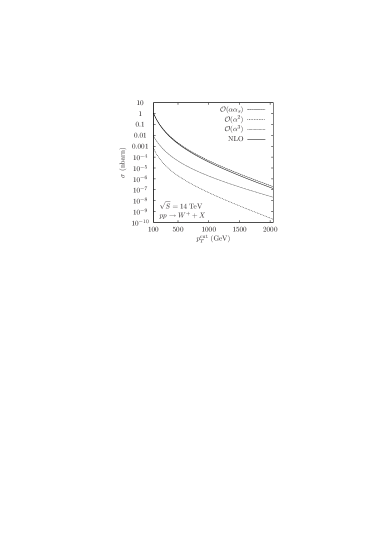
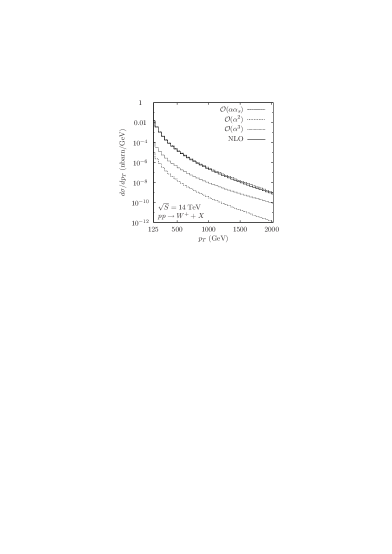
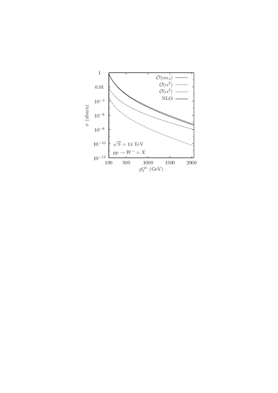
(a)	(b)

Figure 11: (a) Total cross section as a function of $p_{T}^{\mathrm{cut}}$ and (b) $p_{T}$ distribution of $pp\to W^{+}+X$ for $\sqrt{S}=14$ TeV (LHC). The NLO results are compared with those of orders $\mathcal{O}(\alpha\alpha_{s})$, $\mathcal{O}(\alpha^{2})$, and $\mathcal{O}(\alpha^{3})$ via photoproduction.

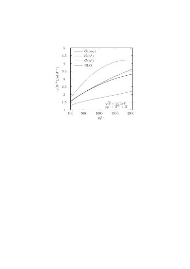
Figure 13: Ratios of the respective results for $W^{+}$ and $W^{-}$ bosons shown in Figs. 11(a) and 12(a).

Let us now discuss the numerical results and their phenomenological implications in detail. Specifically, Figs. 8, 9(a), and 10(a) refer to the Tevatron, while Figs 9(b), 10(b), 11, 12, and 13 refer to the LHC. In Fig. 8(a) the NLO result for the total cross section as a function of $p_{T}^{\mathrm{cut}}$ is compared with the LO contributions of $\mathcal{O}(\alpha\alpha_{s})$ and $\mathcal{O}(\alpha^{2})$ as well as with the photoproduction contribution of $\mathcal{O}(\alpha^{3})$. The $\mathcal{O}(\alpha\alpha_{s})$ and $\mathcal{O}(\alpha^{2})$ results exhibit very similar line shapes, but the normalisation of the latter is suppressed by a factor of about 500. This may be qualitatively understood from the partonic cross section formulae in Eq. (2.21) and by noticing that the $\mathcal{O}(\alpha\alpha_{s})$ contributions from the Compton-like processes (2.3) and (2.4), which have no counterparts in $\mathcal{O}(\alpha^{2})$, are significantly enhanced by the gluon PDF. As a consequence, the LO result is almost entirely exhausted by the $\mathcal{O}(\alpha\alpha_{s})$ contribution.

The inclusion of the NLO correction leads to a moderate reduction in cross section, which increases in magnitude with $p_{T}^{\mathrm{cut}}$, reaching about $-4\%$ for $p_{T}^{\mathrm{cut}}=200$ GeV, as may be seen from Fig. 9(a), where the $K$ factor is depicted.

In Fig. 8(a), also the photoproduction contribution is shown. As explained above, we have to distinguish between elastic and inelastic scattering off the proton on the one hand, and between direct and resolved photons on the other hand, so that, altogether, we have four different contributions, which all formally contribute at $\mathcal{O}(\alpha^{3})$. The resolved-photon contributions turn out to be small against the direct-photon ones and are, therefore, not included in Fig. 9(a). As for the combined direct-photoproduction contribution, we observe from Fig. 8(a), that, except for small values of $p_{T}^{\mathrm{cut}}$, it overshoots the $\mathcal{O}(\alpha^{2})$ contribution, although it is formally suppressed by one power of $\alpha$! Detailed inspection reveals that this unexpected enhancement can be traced to the direct-photoproduction diagram involving the triple-gauge-boson coupling and the space-like $W$-boson exchange, which significantly contributes at large values of $\sqrt{s}$. In fact, for a fixed value of $p_{T}^{\mathrm{cut}}$, the total cross sections of processes (2.6) and (2.7) have an asymptotic large-$s$ behaviour proportional to $1/(m_{T}^{\mathrm{cut}})^{2}$, while those of processes (2.2)–(2.5) behave as $\ln s/s$. Consequently, photoproduction appreciably contributes to the $K$ factor, as is apparent from Fig. 9(a), which also shows the photoproduction to LO ratios for elastic and inelastic scattering. The freedom in the choice of the inelastic photon content of the proton is likely to be the largest source of theoretical uncertainty in the photoproduction cross section. In order to get an idea of this uncertainty, we display in Fig. 9(a) also the inelastic-photoproduction to LO ratio evaluated with the GSV photon spectrum for inelastic scattering. The result is roughly a factor of two smaller than our default prediction based on the MRSTQED04 spectrum.

In Fig. 10(a), we examine the theoretical uncertainties in the $\mathcal{O}(\alpha\alpha_{s})$, $\mathcal{O}(\alpha^{2})$, NLO, and photoproduction results due to the freedom in setting the renormalisation and factorisation scales by exhibiting their $\xi$ dependencies relative to their default values at $\xi=1$. The $\xi$ dependencies of the $\mathcal{O}(\alpha^{2})$ and direct-photoproduction results stem solely from the factorisation scale $M$ and are rather feeble, while those of the $\mathcal{O}(\alpha\alpha_{s})$ and resolved-photoproduction results are also linked to the renormalisation scale $\mu$ of $\alpha_{s}(\mu)$ and are more pronounced, but still not dramatic. The scale variation of the LO result amounts to less than $\pm 15\%$ for $1/2<\xi<2$. It is only slightly reduced by the inclusion of the NLO correction. This is expected because the NLO result is still linear in $\alpha_{s}(\mu)$, so that the $\mu$ dependence of $\alpha_{s}(\mu)$ is not compensated yet.

In Fig. 8(b), the analysis of Fig. 8(a) is repeated for the $p_{T}$ distribution. We observe that the line shapes and relative normalisations of the various distributions are very similar to those in Figs. 8(a) and the same comments apply.

Turning to the LHC, we can essentially repeat the above discussion for the Tevatron, except that we have to take into account the difference between $W^{+}$ and $W^{-}$ boson production. Thus, Fig. 8 has two LHC counterparts, Figs. 11 and 12, for the $W^{+}$ and $W^{-}$ bosons, respectively. To illustrate this difference more explicitly, we show in Fig. 13 the $W^{+}$ to $W^{-}$ ratios of the respective results from Figs. 11 and 12. For simplicity, Figs. 9(b) and 10(b), the LHC counterparts of Figs. 9(a) and 10(a), refer to the averages of the results for $W^{+}$ and $W^{-}$ bosons. In the following, we only focus on those features which are specific for the LHC. From Figs. 11 and 12, we observe that the gaps between the $\mathcal{O}(\alpha\alpha_{s})$ and $\mathcal{O}(\alpha^{2})$ results are increased by about a factor of two, to reach three orders of magnitude. This is mainly because the Compton-like processes (2.3) and (2.4) benefit from the extended dominance of the gluon PDF at small values of $x$. Furthermore, the photoproduction contributions now significantly exceed the $\mathcal{O}(\alpha^{2})$ ones throughout the entire $p_{T}^{\mathrm{cut}}$ and $p_{T}$ ranges. From Fig. 13, we see that the $W^{+}$ to $W^{-}$ ratios take values in excess of unity, as expected, and strongly increase with increasing values of $p_{T}^{\mathrm{cut}}$. Comparing Figs. 9(a) and (b), we find that the $K$ factors are significantly amplified as one passes from the Tevatron to the LHC. This is due to the fact that the Sudakov logarithms, which originate from triangle and box diagrams, become quite sizeable at the large values of $\sqrt{s}$ and $p_{T}$ that can be reached at the LHC. This issue was already dwelled on in Ref. [7], to which we refer the interested reader. Finally, comparing Fig. 10(a) and (b), we conclude that the $\xi$ dependence is generally somewhat smaller at the LHC.

5 Conclusions

We studied the effect of electroweak radiative corrections at first order on the cross section of the inclusive hadroproduction of single $W$ bosons with finite values of $p_{T}$, putting special emphasis on the notion of infrared-save observables with a democratic treatment of hadron jets initiated by (anti)quarks and gluons. This is indispensable because, as a matter of principle, a collinear gluon-photon system cannot be distinguished from a single gluon with the same momentum, so that a minimum-transverse-momentum cut on the gluon is an inadequate tool to prevent a soft-gluon singularity. This led us to include the $\mathcal{O}(\alpha_{s})$ correction to $W+\gamma$ production along with the $\mathcal{O}(\alpha)$ correction to $W+j$ production, both contributing at absolute order $\mathcal{O}(\alpha^{2}\alpha_{s})$. We also considered the contribution from events where one of the colliding hadrons interacts via a real photon, which is of absolute order $\mathcal{O}(\alpha^{3})$. The hadron can then either stay intact (elastic scattering) or be destroyed (inelastic scattering), and the photon can participate in the hard scattering directly (direct photoproduction) or via its quark and gluon content (resolved photoproduction), so that four combinations are possible.

We extracted the UV singularities using dimensional regularisation and removed them by renormalisation in the on-shell scheme. We regularised the soft and collinear IR singularities by means of infinitesimal photon, gluon, and quark masses, $\lambda$, $m_{u}$, and $m_{d}$, respectively. We used the phase-space slicing method, with cuts $\delta_{s}$, $\Delta\vartheta$, and $\Delta\psi$ on the scaled photon and gluon energies and on the separation angles in the initial and final states, respectively, to isolate the soft and collinear singularities within the corrections from real particle radiation. We achieved the cancellation of $\lambda$, $m_{u}$, and $m_{d}$ analytically and ensured that the numerical results are insensitive to variations of $\delta_{s}$, $\Delta\vartheta$, and $\Delta\psi$ within wide ranges about their selected values.

We presented theoretical predictions for the total cross sections with a minimum-$p_{T}$ cut and for the $p_{T}$ distributions to be measured in $p\overline{p}$ collisions with $\sqrt{S}=1.96$ TeV at run II at the Tevatron and in $pp$ collisions with $\sqrt{S}=14$ TeV at the LHC, and estimated the theoretical uncertainties from the scale setting ambiguities. We found that considerably less than 1% of all $W+X$ events contain a prompt photon. The corrections considered turned out to be negative and to increase in magnitude with the value of $p_{T}$. While the reduction is moderate at the Tevatron, reaching about $-4\%$ at $p_{T}=200$ GeV, it can be quite sizeable at the LHC, of order $-30\%$ at $p_{T}=2$ TeV, which is due to the well-known enhancement by Sudakov logarithms. It is an interesting new finding that the photoproduction contribution is considerably larger than expected from the formal order of couplings. In fact, it compensates an appreciable part of the reduction due to the $\mathcal{O}(\alpha^{2}\alpha_{s})$ correction.

Figure 1: Tree-level diagrams of (a) process (2.2) and (b) process (2.5). The tree-level diagrams of processes (2.3), (2.4), (2.6), and (2.7) emerge through crossing.

Figure 2: $\mathcal{O}(\alpha)$ self-energy diagrams of process (2.2).

Figure 3: $\mathcal{O}(\alpha)$ triangle diagrams of process (2.2).

Figure 4: $\mathcal{O}(\alpha)$ box diagrams of process (2.2).

Figure 5: $\mathcal{O}(\alpha)$ counterterm diagrams of process (2.2).

Figure 6: $\mathcal{O}(\alpha_{s})$ self-energy, triangle, and box diagrams of process (2.5).

Figure 7: Tree-level diagrams of process (2.8). The tree-level diagrams of processes (2.9) and (2.10) emerge through crossing.

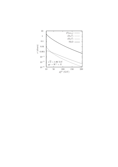
(a)	(b)

Figure 8: (a) Total cross section as a function of $p_{T}^{\mathrm{cut}}$ and (b) $p_{T}$ distribution of $p\overline{p}\to W^{+}+X$ for $\sqrt{S}=1.96$ TeV (Tevatron run II). The NLO results are compared with those of orders $\mathcal{O}(\alpha\alpha_{s})$, $\mathcal{O}(\alpha^{2})$, and $\mathcal{O}(\alpha^{3})$ via photoproduction.

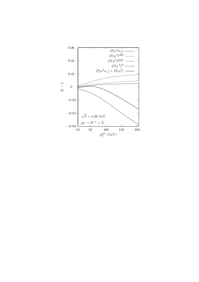
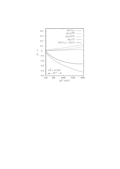
(a)	(b)

Figure 9: NLO corrections ($K-1$), with and without the photoproduction contributions, to the total cross sections of (a) $p\overline{p}\to W^{+}+X$ for $\sqrt{S}=1.96$ TeV (Tevatron run II) and of (b) $pp\to W^{\pm}+X$ for $\sqrt{S}=14$ TeV (LHC) as functions $p_{T}^{\mathrm{cut}}$. For comparison, also the contributions due to elastic and inelastic photoproduction normalised to the LO results are shown. In the latter case, the evaluation is also performed with the GSV PDFs.

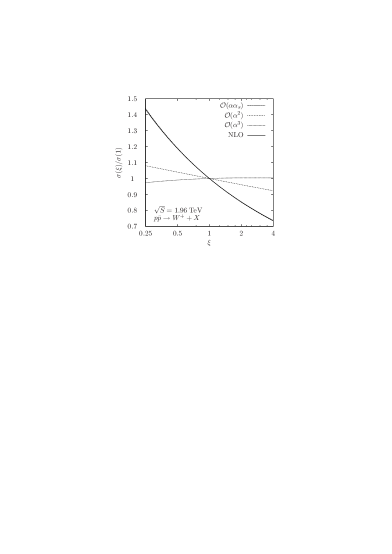
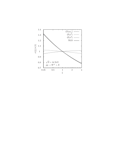
(a)	(b)

Figure 10: Total cross sections of (a) $p\overline{p}\to W^{+}+X$ for $\sqrt{S}=1.96$ TeV and $p_{T}^{\mathrm{cut}}=20$ GeV (Tevatron run II) and of (b) $pp\to W^{\pm}+X$ for $\sqrt{S}=14$ TeV and $p_{T}^{\mathrm{cut}}=200$ GeV (LHC) as functions of $\xi$ normalised to their default values for $\xi=1$. The NLO results are compared with those of orders $\mathcal{O}(\alpha\alpha_{s})$, $\mathcal{O}(\alpha^{2})$, and $\mathcal{O}(\alpha^{3})$ via photoproduction.

(a)	(b)

Figure 12: (a) Total cross section as a function of $p_{T}^{\mathrm{cut}}$ and (b) $p_{T}$ distribution of $pp\to W^{-}+X$ for $\sqrt{S}=14$ TeV (LHC). The NLO results are compared with those of orders $\mathcal{O}(\alpha\alpha_{s})$, $\mathcal{O}(\alpha^{2})$, and $\mathcal{O}(\alpha^{3})$ via photoproduction.

References

-
[1]
UA1 Collaboration, G. Arnison, et al.,
Phys. Lett. B 122 (1983) 103;
UA2 Collaboration, M. Banner, et al., Phys. Lett. B 122 (1983) 476. -
[2]
J. Kubar-Andre, F.E. Paige,
Phys. Rev. D 19 (1979) 221;
K. Harada, T. Kaneko, N. Sakai, Nucl. Phys. B 155 (1979) 169;
K. Harada, T. Kaneko, N. Sakai, Nucl. Phys. B 165 (1980) 545, Erratum;
G. Altarelli, R.K. Ellis, G. Martinelli, Nucl. Phys. B 157 (1979) 461;
P. Aurenche, J. Lindfors, Nucl. Phys. B 185 (1981) 274. -
[3]
R. Hamberg, W.L. van Neerven, T. Matsuura,
Nucl. Phys. B 359 (1991) 343;
R. Hamberg, W.L. van Neerven, T. Matsuura, Nucl. Phys. B 644 (2002) 403, Erratum;
R.V. Harlander, W.B. Kilgore, Phys. Rev. Lett. 88 (2002) 201801. -
[4]
U. Baur, S. Keller, D. Wackeroth,
Phys. Rev. D 59 (1999) 013002;
S. Dittmaier, M. Krämer, Phys. Rev. D 65 (2002) 073007. -
[5]
R.K. Ellis, G. Martinelli, R. Petronzio,
Nucl. Phys. B 211 (1983) 106;
P.B. Arnold, M.H. Reno, Nucl. Phys. B 319 (1989) 37;
P.B. Arnold, M.H. Reno, Nucl. Phys. B 330 (1990) 284, Erratum;
R.J. Gonsalves, J. Pawlowski, C.-F. Wai, Phys. Rev. D 40 (1989) 2245;
F.T. Brandt, G. Kramer, S.L. Nyeo, Int. J. Mod. Phys. A 6 (1991) 3973;
W.T. Giele, E.W.N. Glover, D.A. Kosower, Nucl. Phys. B 403 (1993) 633;
L.J. Dixon, Z. Kunszt, A. Signer, Nucl. Phys. B 531 (1998) 3. -
[6]
C. Anastasiou, L.J. Dixon, K. Melnikov, F. Petriello,
Phys. Rev. D 69 (2004) 094008;
K. Melnikov, F. Petriello, Phys. Rev. Lett. 96 (2006) 231803;
K. Melnikov, F. Petriello, Phys. Rev. D 74 (2006) 114017. - [7] J.H. Kühn, A. Kulesza, S. Pozzorini, M. Schulze, Phys. Lett. B 651 (2007) 160.
- [8] F. Bloch, A. Nordsieck, Phys. Rev. 52 (1937) 54.
-
[9]
T. Kinoshita,
J. Math. Phys. 3 (1962) 650;
T.D. Lee, M. Nauenberg, Phys. Rev. 133 (1964) B1549. - [10] B.A. Kniehl, Phys. Lett. B 254 (1991) 267.
- [11] M. Glück, M. Stratmann, W. Vogelsang, Phys. Lett. B 343 (1995) 399.
- [12] A.D. Martin, R.G. Roberts, W.J. Stirling, R.S. Thorne, Eur. Phys. J. C 39 (2005) 155.
-
[13]
J.D. Bjorken, E.A. Paschos,
Phys. Rev. 185 (1969) 1975;
R.P. Feynman, Phys. Rev. Lett. 23 (1969) 1415. - [14] S. Dittmaier, Ph.D. Thesis, Würzburg, 1993.
-
[15]
J. Küblbeck, M. Böhm, A. Denner,
Comput. Phys. Commun. 60 (1990) 165;
T. Hahn, Comput. Phys. Commun. 140 (2001) 418. - [16] T. Hahn, M. Pẽrez-Victoria, Comput. Phys. Commun. 118 (1999) 153.
- [17] G. Passarino, M. Veltman, Nucl. Phys. B 160 (1979) 151.
- [18] R. Mertig, M. Böhm, A. Denner, Comput. Phys. Commun. 64 (1991) 345.
-
[19]
T. Hahn,
Acta Phys. Polon. B 30 (1999) 3469;
T. Hahn, Nucl. Phys. B (Proc. Suppl.) 89 (2000) 231;
T. Hahn, Nucl. Phys. B (Proc. Suppl.) 157 (2006) 236. - [20] G.J. van Oldenborgh, Comput. Phys. Commun. 66 (1991) 1.
- [21] T. Hahn, Comput. Phys. Commun. 168 (2005) 78.
- [22] A. Sirlin, Phys. Rev. D 22 (1980) 971.
-
[23]
M. Böhm, H. Spiesberger, W. Hollik,
Fortsch. Phys. 34 (1986) 687;
W.F.L. Hollik, Fortsch. Phys. 38 (1990) 165;
A. Denner, Fortsch. Phys. 41 (1993) 307. -
[24]
W. Beenakker, A. Denner,
Nucl. Phys. B 338 (1990) 349;
S. Dittmaier, Nucl. Phys. B 675 (2003) 447. -
[25]
M.L. Ciccolini, S. Dittmaier, M. Krämer,
Phys. Rev. D 68 (2003) 073003;
K.-P.O. Diener, S. Dittmaier, W. Hollik, Phys. Rev. D 69 (2004) 073005. - [26] K.-P.O. Diener, S. Dittmaier, W. Hollik, Phys. Rev. D 72 (2005) 093002.
-
[27]
K. Fabricius, I. Schmitt, G. Kramer, G. Schierholz,
Z. Phys. C 11 (1981) 315;
G. Kramer, B. Lampe, Fortsch. Phys. 37 (1989) 161. -
[28]
N.M. Monyonko, J.H. Reid, M.A. Samuel, G. Tupper,
Z. Phys. C 29 (1985) 381;
F.K. Diakonos, O. Korakianitis, C.G. Papadopoulos, C. Philippides, W.J. Stirling, Phys. Lett. B 303 (1993) 177. - [29] G. ’t Hooft, M. Veltman, Nucl. Phys. B 153 (1997) 365.
- [30] R. Kleiss, Z. Phys. C 33 (1987) 433.
- [31] G. Altarelli, G. Parisi, Nucl. Phys. B 126 (1977) 298.
- [32] J.C. Collins, D.E. Soper, G. Sterman, Adv. Ser. Direct. High Energy Phys. 5 (1988) 1.
- [33] Particle Data Group, W.-M. Yao, et al., J. Phys. G 33 (2006) 1.
- [34] CTEQ Collaboration, J. Pumplin, D.R. Stump, J. Huston, H.-L. Lai, P. Nadolsky, W.-K. Tung, JHEP 0207 (2002) 012.