Renyi Entropy of the XY Spin Chain

Abstract

We consider the one-dimensional $\mathrm{XY}$ quantum spin chain in a transverse magnetic field. We are interested in the Renyi entropy of a block of $\mathrm{L}$ neighboring spins at zero temperature on an infinite lattice. The Renyi entropy is essentially the trace of some power $\alpha$ of the density matrix of the block. We calculate the asymptotic for $\mathrm{L}\to\infty$ analytically in terms of Klein’s elliptic $\lambda$ - function. We study the limiting entropy as a function of its parameter $\alpha$. We show that up to the trivial addition terms and multiplicative factors, and after a proper re-scaling, the Renyi entropy is an automorphic function with respect to a certain subgroup of the modular group; moreover, the subgroup depends on whether the magnetic field is above or below its critical value. Using this fact, we derive the transformation properties of the Renyi entropy under the map $\alpha\to\alpha^{-1}$ and show that the entropy becomes an elementary function of the magnetic field and the anisotropy when $\alpha$ is a integer power of $2$, this includes the purity $tr\rho^{2}$. We also analyze the behavior of the entropy as $\alpha\to 0$ and $\infty$ and at the critical magnetic field and in the isotropic limit [XX model].

1 Introduction

Entanglement is a resource for quantum control [1]. It is necessary for building quantum computers. Different measures of entanglement are used in the literature. For pure systems [considered here] the von Neumann entropy of a subsystem is the most popular measure [2, 3, 4, 5, 6, 7]. The subsystem is a large block of spins in the unique ground state of a spin Hamiltonian. In this paper we evaluate the Renyi entropy of the subsystem. The Renyi entropy was discovered in information theory [8, 9, 10, 11, 12], it is essentially the trace of a power of the density matrix. For physics the Renyi entropy is important, because once we know the value of the trace of every power of the density matrix then we can reconstruct its whole spectrum.

The physical system we consider is the anisotropic $\mathrm{XY}$ model in a transverse magnetic field and the entropy we are interested in is the one of a block of $\mathrm{L}$ neighboring spins at zero temperature and of an infinite system. The Hamiltonian for this model can be written as

$$H=-\sum_{n=-\infty}^{\infty}(1+\gamma)\sigma^{x}_{n}\sigma^{x}_{n+1}+(1-\gamma)\sigma^{y}_{n}\sigma^{y}_{n+1}+h\sigma^{z}_{n}$$ (1)

Here $0<\gamma$ is the anisotropy parameter; $\sigma^{x}_{n}$, $\sigma^{y}_{n}$ and $\sigma^{z}_{n}$ are the Pauli matrices and $0\geq h$ is the magnetic field. The model was solved in [13, 14, 15, 16]. We are going to calculate the bipartite block entropy of the ground state $|GS\rangle$ of the system.

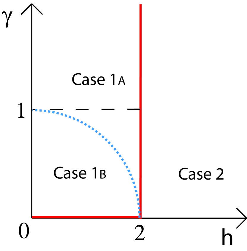
Figure 1: Phase diagram of the anisotropic $XY$ model in a constant magnetic field (only $\gamma\geq 0$ and $h\geq 0$ shown). The three cases $2$, $1$a, $1$b, considered in this paper, are clearly marked. The critical phases ($\gamma=0$, $h\leq 2$ and $h=2$) are drawn in bold lines (red, online). The boundary between cases $1$a and $1$b, where the ground state is given by two degenerate product states, is shown as a dotted line (blue, online). The Ising case ($\gamma=1$) is also indicated, as a dashed line.

The $\mathrm{XY}$ model can be mapped exactly into a system of free fermions with spectrum given by

$$\epsilon_{k}=4\sqrt{\left(\cos k-h/2\right)^{2}+\gamma^{2}\;\sin^{2}k}\;.$$ (2)

We can read the phase diagram of the model from its spectrum and identify that it is critical for $\gamma=0$, $h\leq 2$ (corresponding to the isotropic $\mathrm{XY}$ model, or $\mathrm{XX}$ model) and at the critical magnetic field $h=h_{c}=2$. For $h=h_{f}(\gamma)=2\sqrt{1-\gamma^{2}}$ (factorizing field) the ground state can be written as a product state, as it was found in [17], and is doubly degenerate:

$$|GS_{1}\rangle = \prod_{n\in\mbox{\rm lattice}}\left[\cos(\theta)|\uparrow_{n}\rangle+\sin(\theta)|\downarrow_{n}\rangle\right]\;,$$

$$|GS_{2}\rangle = \prod_{n\in\mbox{\rm lattice}}\left[\cos(\theta)|\uparrow_{n}\rangle-\sin(\theta)|\downarrow_{n}\rangle\right]\;,$$ (3)

where $\cos^{2}(2\theta)=(1-\gamma)/(1+\gamma)$. Off this line, the ground state of the model $|GS\rangle$ is in continuity with the state

$$|GS\rangle_{h=h_{f}(\gamma)}=|GS_{1}\rangle+|GS_{2}\rangle\;.$$ (4)

The line $h=h_{f}(\gamma)$ is not a phase transition, but the entropy has a weak singularity across it, since its derivative, although finite, is discontinuous. In Fig. 1 we show the phase diagram of the $\mathrm{XY}$ model and mark the three regions where we calculate the different expressions of the entropy.

We shall calculate the entropy of a block of $L$ neighboring spins (a subsystem) of the ground state $|GS\rangle$ as a measure of the entanglement between this block and the rest of the chain. We treat the whole chain as a binary system $|GS\rangle=|A\&B\rangle$. We denote this block of $L$ neighboring spins by subsystem A and the rest of the chain by subsystem B. The density matrix of the ground state can be denoted by $\rho_{AB}=|GS\rangle\langle GS|$. The reduced density matrix of subsystem A is $\rho_{A}=Tr_{B}(\rho_{AB})$. Then, the von Neumann entropy $S(\rho_{A})$ and the Rényi entropy $S_{\alpha}(\rho_{A})$ of the block of spins can be evaluated by the expression

$$S(\rho_{A}) = -Tr(\rho_{A}\ln\rho_{A}),$$ (5)

$$S_{\alpha}(\rho_{A}) = \frac{1}{1-\alpha}\ln Tr(\rho_{A}^{\alpha}),\qquad\alpha\neq 1~{}~{}\textrm{and}~{}~{}\alpha>0.$$ (6)

Here the power $\alpha$ is a parameter. When evaluated for 1-dimensional critical theories, these entropies diverge logarithmically with the size of the block, while they saturate to a constant in the presence of a gap [18].

For the isotropic version of the XY model $\gamma=0$ we evaluated Rényi entropy of a large block of spins in [19]. The von Neumann entropy of the block in the XY model was calculated in [20, 21, 22, 23]. The methods of Toeplitz determinants [24, 25, 26, 27, 28, 29], as well as the techniques based on integrable Fredholm operators[30, 31, 32], have been used for the evaluation of the von Neumann entropy of this model [19, 33].

In this paper we evaluate the Rényi entropy, which is the natural generalization of the von Neumann entropy [8]. When $\alpha\to 1$, the Rényi entropy turns into the von Neumann entropy.

2 Renyi Entropy.

The von Neumann Entropy of the block of spins has been calculated in [33] and [7]. We shall use the same notations and introduce an elliptic parameter:

$$k=\left\{\begin{array}[]{l}\sqrt{(h/2)^{2}+\gamma^{2}-1}\;/\;\gamma,\;\;\;\;\;\;\;\;\;\;\;\;\;\;\;\;\mbox{Case 1a:~{}$4(1-\gamma^{2})<h^{2}<4$;}\\[8.5359pt] \sqrt{({1-h^{2}/4-\gamma^{2}})/({1-h^{2}/4})}\;,\;\;\;\mbox{Case 1b:~{}$h^{2}<4(1-\gamma^{2})$;}\\[8.5359pt] \gamma\;/\;\sqrt{(h/2)^{2}+\gamma^{2}-1},\;\;\;\;\;\;\;\;\;\;\;\;\;\;\;\;\mbox{Case 2~{}:~{}$h>2$.}\end{array}\right.$$ (10)

We shall also use the complete elliptic integral of the first kind

$$I(k)=\int_{0}^{1}\frac{dx}{\sqrt{(1-x^{2})(1-k^{2}x^{2})}}$$ (11)

and the modulus

$$\tau_{0}=I(k^{\prime})/I(k),\qquad\qquad k^{\prime}=\sqrt{1-k^{2}},$$ (12)

as well as:

$$\epsilon\equiv\pi\tau_{0},\qquad q\equiv{\rm e}^{-\epsilon}={\rm e}^{-\pi I(k^{\prime})/I(k)}.$$ (13)

We will need the following identities as well [34]:

$$\prod_{m=0}^{\infty}\left(1+q^{2m+1}\right)=\left({16q\over k^{2}k^{\prime 2}}\right)^{1/24}$$ (14)

$$\prod_{m=1}^{\infty}\left(1+q^{2m}\right)=\left({k^{2}\over 16qk^{\prime}}\right)^{1/12}.$$ (15)

Now let us start the evaluation of the Renyi entropy of a block of $L$ neighboring spins. It can be represented [19] as

$$S_{R}(\rho_{A},\alpha)={1\over 1-\alpha}\sum_{k=1}^{L}\ln\left[\left({1+\nu_{k}\over 2}\right)^{\alpha}+\left({1-\nu_{k}\over 2}\right)^{\alpha}\right],$$ (16)

where the numbers

$$\pm i\nu_{k},\quad k=1,...,L$$

are the eigenvalues of a certain block Toeplitz matrix. In [33] it is shown that in the large $L$ limit the eigenvalues $\nu_{2m}$ and $\nu_{2m+1}$ merge to the number $\lambda_{m}$ defined below in eq (18),

$$\nu_{2m},\nu_{2m+1}\to\lambda_{m}.$$

Hence, the Renyi entropy in the large $L$ limit can be identified with the convergent series,

$$S_{R}(\rho_{A},\alpha)={1\over 1-\alpha}\sum_{m=-\infty}^{\infty}\ln\left[\left({1+\lambda_{m}\over 2}\right)^{\alpha}+\left({1-\lambda_{m}\over 2}\right)^{\alpha}\right],$$ (17)

with

$$\lambda_{m}=\tanh\left(m+\frac{1-\sigma}{2}\right)\pi\tau_{0}.$$ (18)

The summation of the series can be done following the same approach as in the case of the von Neuman entropy (cf. [7]).

2.1 $h>2$

With $\epsilon\equiv\pi\tau_{0}$, we have

$$1+\lambda_{m} = 2{1\over 1+{\rm e}^{-(1+2m)\epsilon}}$$ (19)

$$1-\lambda_{m} = 2{{\rm e}^{-(1+2m)\epsilon}\over 1+{\rm e}^{-(1+2m)\epsilon}}.$$ (20)

Then, the entropy is:

$$S_{R} = {1\over 1-\alpha}\sum_{m=-\infty}^{\infty}\ln\left[\left({1\over 1+{\rm e}^{-(1+2m)\epsilon}}\right)^{\alpha}+\left({{\rm e}^{-(1+2m)\epsilon}\over 1+{\rm e}^{-(1+2m)\epsilon}}\right)^{\alpha}\right]$$ (21)

$$= {2\over 1-\alpha}\sum_{m=0}^{\infty}\ln\left[\left({1\over 1+{\rm e}^{-(1+2m)\epsilon}}\right)^{\alpha}+\left({{\rm e}^{-(1+2m)\epsilon}\over 1+{\rm e}^{-(1+2m)\epsilon}}\right)^{\alpha}\right]$$

$$= {2\over 1-\alpha}\sum_{m=0}^{\infty}\ln\left[{1+{\rm e}^{-\alpha(1+2m)\epsilon}\over\left(1+{\rm e}^{-(1+2m)\epsilon}\right)^{\alpha}}\right]$$

$$= {2\over 1-\alpha}\sum_{m=0}^{\infty}\ln\left[1+{\rm e}^{-\alpha(1+2m)\epsilon}\right]-{2\alpha\over 1-\alpha}\sum_{m=0}^{\infty}\ln\left[1+{\rm e}^{-(1+2m)\epsilon}\right].$$

Summing the second term is straightforward, using (14):

$$\hskip-28.45274pt-{2\alpha\over 1-\alpha}\sum_{m=0}^{\infty}\ln\left[1+{\rm e}^{-(1+2m)\epsilon}\right] = -{2\alpha\over 1-\alpha}\ln\prod_{m=0}^{\infty}\left(1+q^{2m+1}\right)$$ (22)

$$= -{1\over 12}{\alpha\over 1-\alpha}\;\left[\ln q+\ln\left({16\over k^{2}k^{\prime 2}}\right)\right],$$

where, as usual,

$$q\equiv{\rm e}^{-\pi I(k^{\prime})/I(k)}.$$ (23)

In order to sum up the first term we notice that identity (14) can be interpreted as the evaluation of the product in the left hand side in terms of the function $k\equiv k(q)$ defined implicitly by equation (23). A fundamental fact of the theory of elliptic functions is that the function $k(q)$ admits an explicit representation in terms of the theta-constants. Indeed, the following formulae take place (see e.g. [34]):

$$\hskip-28.45274ptk(q)={\theta_{2}^{2}(0,q)\over\theta_{3}^{2}(0,q)}\;,\qquad\qquad k^{\prime}(q)={\theta_{4}^{2}(0,q)\over\theta_{3}^{2}(0,q)}\;,$$ (24)

where $\theta_{j}(z|q)$, $j=1,2,3,4$ are the Jacobi theta-functions. We remind (see again [34]) that the theta functions are defined for any $|q|<1$ by the following Fourier series

$$\theta_{1}(z,q)=i\sum_{n=-\infty}^{\infty}(-1)^{n}q^{\left(\frac{2n-1}{2}\right)^{2}}e^{2iz\left(n-\frac{1}{2}\right)}\;,$$ (25)

$$\theta_{2}(z,q)=\sum_{n=-\infty}^{\infty}q^{\left(\frac{2n-1}{2}\right)^{2}}e^{2iz\left(n-\frac{1}{2}\right)}\;,$$ (26)

$$\theta_{3}(z,q)=\sum_{n=-\infty}^{\infty}q^{n^{2}}e^{2izn}\;,$$ (27)

$$\theta_{4}(z,q)=\sum_{n=-\infty}^{\infty}(-1)^{n}q^{n^{2}}e^{2izn}\;.$$ (28)

In particular, it follows that the functions

$$k^{\prime}(q)\quad\mbox{and}\quad q^{-1/2}k(q)\;,$$ (29)

are analytic on the unit disc $|q|<1$. It is also worth mentioning the classical formula for the integral $I(k)$,

$$I(k)=\frac{\pi}{2}\theta_{3}^{2}(0,q).$$ (30)

Put now,

$$k_{\alpha}:=k(q^{\alpha})\;,$$ (31)

where $q$ is the $q$ - parameter corresponding via (23) to the original elliptic parameter $k$ from (10). Then for the first term in (21) we will have

$$\hskip-28.45274pt{2\over 1-\alpha}\sum_{m=0}^{\infty}\ln\left[1+{\rm e}^{-\alpha(1+2m)\epsilon}\right] = {2\over 1-\alpha}\ln\prod_{m=0}^{\infty}\left(1+(q^{\alpha})^{2m+1}\right)$$ (32)

$$= {1\over 12}{1\over 1-\alpha}\;\left[\alpha\ln q+\ln\left({16\over k^{2}_{\alpha}k^{\prime 2}_{\alpha}}\right)\right].$$

Substituting this expression together with (22) into (21), we arrive at the equation,

$$S_{R}=\frac{1}{12}\frac{1}{1-\alpha}\ln\left(\frac{16}{k^{2}_{\alpha}k^{\prime 2}_{\alpha}}\right)-\frac{1}{12}\frac{\alpha}{1-\alpha}\ln\left(\frac{16}{k^{2}k^{\prime 2}}\right)$$

$$=\frac{1}{6}\frac{\alpha}{1-\alpha}\ln(kk^{\prime})-\frac{1}{6}\frac{1}{1-\alpha}\ln(k_{\alpha}k^{\prime}_{\alpha})+{1\over 3}\ln 2,$$ (33)

which in turns yields the following final expression for the Renyi entropy.

$$\hskip-42.67912ptS_{R}(\rho_{A},\alpha)={1\over 6}\;{\alpha\over 1-\alpha}\;\ln\left(k\;k^{\prime}\right)-{1\over 3}\;{1\over 1-\alpha}\;\ln\left({\theta_{2}(0,q^{\alpha})\;\theta_{4}(0,q^{\alpha})\over\theta_{3}^{2}(0,q^{\alpha})}\right)\;+{1\over 3}\ln 2.$$ (34)

Here, the elliptic parameter $k$ is defined in (10), $k^{\prime}=\sqrt{1-k^{2}}$, the modulus parameter $q$ is given by equation (23) where $I(k)$ is the complete elliptic integral (11), and the theta functions $\theta_{j}(z,q)$ are defined by the series (25 - 28).

2.2 $h<2$

In this case we have

$$\lambda_{m}=\tanh(m\pi\tau_{0})={{\rm e}^{2m\epsilon}-1\over{\rm e}^{2m\epsilon}+1},$$ (35)

where, as usual,

$$\epsilon\equiv\pi\tau_{0}.$$ (36)

The entropy is:

$$S_{R} = {1\over 1-\alpha}\sum_{m=-\infty}^{\infty}\ln\left[\left({1\over 1+{\rm e}^{-2m\epsilon}}\right)^{\alpha}+\left({{\rm e}^{-2m\epsilon}\over 1+{\rm e}^{-2m\epsilon}}\right)^{\alpha}\right]$$ (37)

$$= {2\over 1-\alpha}\sum_{m=1}^{\infty}\ln\left[\left({1\over 1+{\rm e}^{-2m\epsilon}}\right)^{\alpha}+\left({{\rm e}^{-2m\epsilon}\over 1+{\rm e}^{-2m\epsilon}}\right)^{\alpha}\right]+{1\over 1-\alpha}\ln\left(2{1\over 2^{\alpha}}\right)$$

$$= {2\over 1-\alpha}\sum_{m=1}^{\infty}\ln\left[1+{\rm e}^{-2\alpha m\epsilon}\right]-{2\alpha\over\alpha-1}\sum_{m=1}^{\infty}\ln\left[1+{\rm e}^{-2m\epsilon}\right]+\ln 2.$$

Again the second term can be immediately summed using (15):

$$-{2\alpha\over 1-\alpha}\sum_{m=1}^{\infty}\ln\left[1+{\rm e}^{-2m\epsilon}\right] = -{2\alpha\over 1-\alpha}\ln\prod_{m=1}^{\infty}\left(1+q^{2m}\right)$$ (38)

$$= -{1\over 6}{\alpha\over 1-\alpha}\left[\ln\left({k^{2}\over 16k^{\prime}}\right)-\ln q\right],$$

where, as usual,

$$q\equiv{\rm e}^{-\pi I(k^{\prime})/I(k)}.$$ (39)

The first term, as in the previous case, admits the similar representation involving the elliptic parameter $k_{\alpha}\equiv k(q^{\alpha})$,

$${2\over 1-\alpha}\sum_{m=1}^{\infty}\ln\left[1+{\rm e}^{-2\alpha m\epsilon}\right]={1\over 6}{1\over\alpha-1}\left[\ln\left({k^{2}_{\alpha}\over 16k^{\prime}_{\alpha}}\right)-\alpha\ln q\right].$$ (40)

Using (38) and (40) in (37), we obtained that

$$S_{R} = \frac{1}{6}\frac{1}{1-\alpha}\ln\left(\frac{k^{2}_{\alpha}}{16k^{\prime}_{\alpha}}\right)-\frac{1}{6}\frac{\alpha}{1-\alpha}\ln\left(\frac{k^{2}}{16k^{\prime}}\right)+\ln 2$$ (41)

$$= \frac{1}{6}\frac{\alpha}{1-\alpha}\ln\left(\frac{k^{\prime}}{k^{2}}\right)+\frac{1}{6}\frac{1}{1-\alpha}\ln\left(\frac{k_{\alpha}^{2}}{k^{\prime}_{\alpha}}\right)+{1\over 3}\ln 2,$$

which in turns yields the following final expression for the Renyi entropy in the case $h<2$.

$$\hskip-42.67912ptS_{R}(\rho_{A},\alpha)={1\over 6}\;{\alpha\over 1-\alpha}\;\ln\left({k^{\prime}\over k^{2}}\right)+{1\over 3}\;{1\over 1-\alpha}\;\ln\left({\theta_{2}^{2}(0,q^{\alpha})\over\theta_{3}(0,q^{\alpha})\;\theta_{4}(0,q^{\alpha})}\right)+{1\over 3}\ln 2.$$ (42)

Here, as before, the elliptic parameter $k$ is defined in (10), $k^{\prime}=\sqrt{1-k^{2}}$, the modulus parameter $q$ is given by equation (23) where $I(k)$ is the complete elliptic integral (11), and the theta functions $\theta_{j}(z|q)$ are defined by the series (25 - 28).

Remark. One can wonder about an apparent tautological character of the formulae (34) and (42). Indeed, they seem just to re-express one $q$-series ($S_{R}(\rho_{A},\alpha)$) in terms of the another ($\theta_{j}(0|q)$). The important point however is that the $q$-series representing the theta-constants place the object of interest, i.e. the Renyi entropy, in the well - developed realm of classical elliptic functions. In fact, to solve a problem in terms of Jacobi theta- function is as good as to solve it in terms of, say, elementary exponential function (after all, the exponential function is also an infinite series !). The crucial thing is that a lot is known about the properties of the theta-constants and this allows a quite comprehensive study of the Renyi entropy both numerically and analytically. In the next section we will demonstrate the efficiency of equations (34) and (42).

3 Renyi Entropy. The Analysis.

When studying the analytic properties of the Renyi entropy with respect to the variable $\alpha$, it is convenient to pass from the modulus parameter $q$ to the (more standard) modulus parameter $\tau$ defined by the relations,

$$q=e^{\pi i\tau},\quad\tau=i\frac{I(k^{\prime})}{I(k)}\equiv i\tau_{0},\quad\Im\tau>0.$$ (43)

The theta functions $\theta_{j}(z,q)$ then become the functions,

$$\theta_{j}(z|\tau):=\theta_{j}(z,e^{\pi i\tau}),\quad j=1,2,3,4,$$ (44)

which are holomorphic for all $z$ and for all $\tau$ from the upper half plane,

$$\Im\tau>0.$$ (45)

Using these new notations, the above obtain formulae for the Renyi entropy can be rewritten as

$$\hskip-56.9055ptS_{R}(\rho_{A},\alpha)={1\over 6}\;{\alpha\over 1-\alpha}\;\ln\left(k\;k^{\prime}\right)-{1\over 3}\;{1\over 1-\alpha}\;\ln\left({\theta_{2}(0|\alpha i\tau_{0})\;\theta_{4}(0|\alpha i\tau_{0})\over\theta_{3}^{2}(0|\alpha i\tau_{0})}\right)\;+{1\over 3}\ln 2,$$ (46)

for $h>2$ and

$$\hskip-56.9055ptS_{R}(\rho_{A},\alpha)={1\over 6}\;{\alpha\over 1-\alpha}\;\ln\left({k^{\prime}\over k^{2}}\right)+{1\over 3}\;{1\over 1-\alpha}\;\ln\left({\theta_{2}^{2}(0|\alpha i\tau_{0})\over\theta_{3}(0|\alpha i\tau_{0})\;\theta_{4}(0|\alpha i\tau_{0})}\right)+{1\over 3}\ln 2,$$ (47)

for $h<2$. To proceed with the analysis of these expressions as functions of $\alpha$, we will need some pieces of the general theory of Jacobi functions $\theta_{j}(z|\tau)$ which we collect in Appendix A.

Our first observation is that the domain of analyticity (45) and the positiveness of the parameter $\tau_{0}$ indicate that the all three theta-constants, i.e. $\theta_{2}(0|\alpha i\tau_{0})$, $\theta_{3}(0|\alpha i\tau_{0})$, and $\theta_{4}(0|\alpha i\tau_{0})$ are analytic in the right half plane of the complex $\alpha$ - plane:

$$\Re\alpha>0.$$ (48)

Simultaneously we notice that inequality (114) implies that the theta-ratios appearing in the right hand sides of (46) and (47) are never zero. Hence we can claim that the Renyi entropy, as a function of $\alpha$, is analytic in the right half plane (48), with the possible pole at $\alpha=1$. However, since as $\alpha\to 1$ the theta-ratios in (46) and (47) become the square roots of the product $kk^{\prime}$ and of the ratio $k^{2}/k^{\prime}$, respectively (see also (33) and (41)), the singularity at $\alpha=1$ is, in fact, removable and we can write that

$$S_{R}(\rho_{A},1)=-\frac{1}{6}\ln(kk^{\prime})+\frac{1}{3}\ln 2+\frac{1}{3}\frac{d}{d\alpha}\ln\left({\theta_{2}(0|\alpha i\tau_{0})\;\theta_{4}(0|\alpha i\tau_{0})\over\theta_{3}^{2}(0|\alpha i\tau_{0})}\right)_{\alpha=1}$$

$$\equiv-\frac{1}{6}\ln(kk^{\prime})+\frac{1}{3}\ln 2+\frac{1}{6}\frac{d}{d\alpha}\ln(k_{\alpha}k^{\prime}_{\alpha})|_{\alpha=1}$$ (49)

for $h>2$ and

$$S_{R}(\rho_{A},1)=-\frac{1}{6}\ln\left(\frac{k^{\prime}}{k^{2}}\right)+\frac{1}{3}\ln 2+\frac{1}{3}\frac{d}{d\alpha}\ln\left({\theta_{3}(0|\alpha i\tau_{0})\;\theta_{4}(0|\alpha i\tau_{0})\over\theta_{2}^{2}(0|\alpha i\tau_{0})}\right)_{\alpha=1}$$

$$\equiv-\frac{1}{6}\ln\left(\frac{k^{\prime}}{k^{2}}\right)+\frac{1}{3}\ln 2+\frac{1}{6}\frac{d}{d\alpha}\ln\left(\frac{k^{\prime}_{\alpha}}{k^{2}_{\alpha}}\right)|_{\alpha=1}$$ (50)

for $h<2$. It is an exercise in the theory of elliptic functions to show that the expressions on the right hand sides of (49) and (50) are in fact the respective Von Neumann entropies calculated in [19, 33, 7]:

$${\hskip-28.45274pt}S(\rho_{A})=\frac{1}{6}\left[\;\ln{\frac{4}{k\;k^{\prime}}}+(k^{2}-k^{\prime 2})\frac{2I(k)I(k^{\prime})}{\pi}\right]\;, h>2\;;$$ (51)

$${\hskip-28.45274pt}S(\rho_{A})=\frac{1}{6}\left[\;\ln{\left(\frac{4k^{2}}{k^{\prime}}\right)}+\left(2-k^{2}\right)\frac{2I(k)I(k^{\prime})}{\pi}\right]\;, h<2\;.$$ (52)

This fact, i.e. the statement that

$$\lim_{\alpha\to 1}S_{R}(\rho_{A},\alpha)=S(\rho_{A})\;,$$ (53)

can be of course obtained via much more elementary calculations based on the original series representation (17) for $S_{R}(\rho_{A},\alpha)$.

Consider now the two other critical cases: $\alpha\to 0$ and $\alpha\to\infty$.

3.1 $\alpha\to\infty$

The limit of large $\alpha$ is interesting for the single copy entanglement suggested by M. Plenio and J. Eisert[35]. In fact, the Renyi entropy contains information about all eigenvalues of the density matrix and we can extract the largest eigenvalue [maximum probability $p_{M}$] from the limit $\alpha\to\infty$ ($S_{\alpha}(\rho_{A})\to-\ln p_{M}$).

Using the first series from equations (111) - (113) we obtain at once that

$$\frac{\theta_{2}(0|\alpha i\tau_{0})\theta_{4}(0|\alpha i\tau_{0})}{\theta^{2}_{3}(0|\alpha i\tau_{0})}=2e^{-\frac{\pi\alpha\tau_{0}}{4}}\left(1+O\left(e^{-\alpha\pi\tau_{0}}\right)\right)$$ (54)

and

$$\frac{\theta^{2}_{2}(0|\alpha i\tau_{0})}{\theta_{3}(0|\alpha i\tau_{0})\theta_{4}(0|\alpha i\tau_{0})}=4e^{-\frac{\pi\alpha\tau_{0}}{2}}\left(1+O\left(e^{-2\alpha\pi\tau_{0}}\right)\right),$$ (55)

as $\alpha\to\infty$, $-\pi/2<\arg\alpha<\pi/2$. Plugging these estimates in (46) and (47) and recalling that $\tau_{0}=I(k^{\prime})/I(k)$, we arrive at the following description of the Renyi entropy in the large $\alpha$ limit.

$$S_{R}(\rho_{A},\alpha)=\frac{\alpha}{1-\alpha}\left(\frac{1}{6}\ln\frac{kk^{\prime}}{4}+\frac{\pi}{12}\frac{I(k^{\prime})}{I(k)}\right)$$ (56)

$$+O\left(\frac{1}{\alpha}e^{-\alpha\pi\tau_{0}}\right)$$

$$=-\frac{1}{6}\ln\frac{kk^{\prime}}{4}+\frac{\pi}{12}\frac{I(k^{\prime})}{I(k)}+O\left(\frac{1}{\alpha}\right),$$

$$\alpha\to\infty,\quad-\frac{\pi}{2}<\arg\alpha<\frac{\pi}{2},$$

for $h>2$, and

$$S_{R}(\rho_{A},\alpha)=\frac{\alpha}{1-\alpha}\left(\frac{1}{6}\ln\frac{k^{\prime}}{4k^{2}}-\frac{\pi}{6}\frac{I(k^{\prime})}{I(k)}\right)+\frac{1}{1-\alpha}\ln 2$$ (57)

$$+O\left(\frac{1}{\alpha}e^{-2\alpha\pi\tau_{0}}\right)$$

$$=-\frac{1}{6}\ln\frac{k^{\prime}}{4k^{2}}+\frac{\pi}{6}\frac{I(k^{\prime})}{I(k)}+O\left(\frac{1}{\alpha}\right),$$

$$\alpha\to\infty,\quad-\frac{\pi}{2}<\arg\alpha<\frac{\pi}{2},$$

for $h<2$. Alternatively, these estimates can be easily extracted from the original series representations, i.e. equations (21) and (37), with the help of the identities (14) and (15). In other words, the theta-summation of the series (21) and (37) is not really needed for the large values of the parameter $\alpha$.

Remark. The asymptotic representations (56) and (57) are only valid for the bulk of the $XY$ model, i.e. away from critical lines $\gamma=0$ or $h=2$. Near the critical points, when $\gamma\neq 0$ and $h\to 2$, or $\gamma\to 0$ and $h<2$, the module parameter $\tau_{0}$ becomes small and the estimates (56) and (57) are not valid unless the double scaling condition,

$$\alpha\tau_{0}\to\infty$$ (58)

takes place.

3.2 $\alpha\to 0$

This is where the theta-formulae help. Indeed, using the second series from the Jacobi identities (111) - (113), we arrive at the estimates,

$$\frac{\theta_{2}(0|\alpha i\tau_{0})\theta_{4}(0|\alpha i\tau_{0})}{\theta^{2}_{3}(0|\alpha i\tau_{0})}=2e^{-\frac{\pi}{4\alpha\tau_{0}}}\left(1+O\left(e^{-\frac{\pi}{\alpha\tau_{0}}}\right)\right)$$ (59)

and

$$\frac{\theta^{2}_{2}(0|\alpha i\tau_{0})}{\theta_{3}(0|\alpha i\tau_{0})\theta_{4}(0|\alpha i\tau_{0})}=\frac{1}{2}e^{\frac{\pi}{4\alpha\tau_{0}}}\left(1+O\left(e^{-\frac{\pi}{\alpha\tau_{0}}}\right)\right)$$ (60)

as $\alpha\>\tau_{0}\to 0$, $-\pi/2<\arg\alpha<\pi/2$. These formulae indicate the appearance of a singularity of order $\alpha^{-1}$ in the Renyi entropy as $\alpha\to 0$. In fact, since we consider the limit of a large block of spins, the dimension of the corresponding Hilbert space also goes to infinity. This is the reason for which the Renyi entropy has a singularity at $\alpha=0$.

Substituting (59) and (60) into (46) and (47), respectively, we obtain the following description of the Renyi entropy in the small $\alpha$ limit.

$$S_{R}(\rho_{A},\alpha)=\frac{1}{\alpha(1-\alpha)}\frac{\pi}{12}\frac{I(k)}{I(k^{\prime})}+\frac{\alpha}{1-\alpha}\frac{1}{6}\ln\frac{kk^{\prime}}{4}+O\left(e^{-\frac{\pi}{\alpha\tau_{0}}}\right)$$ (61)

$$=\frac{1+\alpha}{\alpha}\frac{\pi}{12}\frac{I(k)}{I(k^{\prime})}+O(\alpha),$$ (62)

$$\alpha\to 0,\quad-\frac{\pi}{2}<\arg\alpha<\frac{\pi}{2},$$

for $h>2$, and

$$S_{R}(\rho_{A},\alpha)=\frac{1}{\alpha(1-\alpha)}\frac{\pi}{12}\frac{I(k)}{I(k^{\prime})}+\frac{\alpha}{1-\alpha}\frac{1}{6}\ln\frac{k^{\prime}}{4k^{2}}+O\left(e^{-\frac{\pi}{\alpha\tau_{0}}}\right)$$ (63)

$$=\frac{1+\alpha}{\alpha}\frac{\pi}{12}\frac{I(k)}{I(k^{\prime})}+O(\alpha),$$ (64)

$$\alpha\to 0,\quad-\frac{\pi}{2}<\arg\alpha<\frac{\pi}{2},$$

for $h<2$.

Similar to the case of the Von Neumann entropy dealt with in [33], equations (61) and (63) can be also used for the evaluation of the small $\tau_{0}\equiv I(k^{\prime})/I(k)$ limit of the Renyi entropy with the fixed $\alpha>0$. This limit (cf. [33]) appears either in the case of the critical magnetic field, i.e. $\gamma\neq 0$ and $h\to 2$, or when approaching the $XX$ model, i.e. $\gamma\to 0$ and $h<2$. We shall now consider these limits.

3.3 Critical magnetic field: $\gamma\neq 0$ and $h\to 2$

This is included in Case 1a and Case 2 which means that,

$$\hskip-28.45274ptk=1-\frac{1}{2\gamma^{2}}|h-2|+O(|h-2|^{2}),\quad k^{\prime}=\frac{1}{\gamma}|h-2|^{2}\left(1+O(|h-2|)\right),$$ (65)

and, in turn,

$$\pi\frac{I(k)}{I(k^{\prime})}=-\ln|2-h|+2\ln 4\gamma+O(|h-2|\ln^{2}|h-2|),$$ (66)

$$\quad h\to 2,\quad\gamma\neq 0.$$

This means that in this limit $\tau_{0}\to 0$ and we can use (61) to arrive at the following estimates for the Renyi entropy in the case of the critical magnetic field,

$$S_{R}(\rho_{A},\alpha)=\frac{1+\alpha}{\alpha}\Bigl{(}-\frac{1}{12}\ln|2-h|+\frac{1}{6}\ln 4\gamma\Bigr{)}$$ (67)

$$+O(|h-2|\ln^{2}|h-2|).$$

We notice that the singularity of the Renyi entropy is logarithmic like for the Von Neumann entropy, but coefficient in front of the logarithm is different and $\alpha$-dependent.

3.4 An approach to $XX$ model: $\gamma\to 0$ and $h<2$

This is included in Case 1b which means that,

$$k=1-\frac{2\gamma^{2}}{4-h^{2}}+O(\gamma^{4}),\quad k^{\prime}=\frac{2\gamma}{\sqrt{4-h^{2}}}\left(1+O(\gamma^{2})\right),$$ (68)

and, in turn,

$$\pi\frac{I(k)}{I(k^{\prime})}=-2\ln\gamma+\ln(4-h^{2})+2\ln 2+O(\gamma\ln^{2}\gamma),$$ (69)

$$\gamma\to 0,\quad h<2\sqrt{1-\gamma^{2}}.$$

Again, since $\tau_{0}\to 0$, we can substitute these into (63) and arrive at the following estimates for the Renyi intropy in the case of the XX model limit

$$S_{R}(\rho_{A},\alpha)=\frac{1+\alpha}{\alpha}\Bigl{(}-\frac{1}{6}\ln\gamma+\frac{1}{12}\ln(4-h^{2})+\frac{1}{6}\ln 2\Bigr{)}$$ (70)

$$+O(\gamma\ln^{2}\gamma).$$

We note that if $\alpha=1$ then equations (67) and (70) transforms to the respective formulae for the Neumann entropy obtained earlier in [33].

3.5 The factorizing field

We already showed in the introduction that for $h=h_{f}(\gamma)=2\sqrt{1-\gamma^{2}}$ the ground state can be written as

$$|GS\rangle=|GS_{1}\rangle+|GS_{2}\rangle\;,$$ (71)

where $|GS_{1,2}\rangle$ are the product states given in (3) and clearly have no entropy/entanglement by themselves.

We can calculate the Renyi entropy of the ground state at the factorizing field by considering the limit $k\to 0$ of (47). Remembering that, using (111-113) in this limit

$$\theta_{2}(0|\alpha{\rm i}\tau\sim 0) \sim 2\left({k\over 4}\right)^{\alpha/2}\;,$$ (72)

$$\theta_{3}(0|\alpha{\rm i}\tau\sim 0) \sim \theta_{4}(0|\alpha{\rm i}\tau\sim 0)\sim 1\;,$$ (73)

it is easy to show that

$$S_{R}(\rho_{A},\alpha)=\ln 2$$ (74)

regardless the value of $\alpha$. This result is not surprising and was to be expected in light of (71). In fact, the limiting density matrix of the block of spins at the factorizing field is $(1/2)\times I_{2}$, where $I_{2}$ is the $2\times 2$ Identical matrix.

Please note the importance of the order of limits around the factorizing field. In fact, the expression in (74) is independent of $\alpha$ and therefore regular in the limit $\alpha\to 0$, while off the factorizing field line the entropy diverges like in (64) for $\alpha\to 0$. As one approaches the factorizing field, $k\to 0$ and therefore $\tau_{o}\to\infty$ in such a way that $\alpha\tau_{0}$ stays constant.

4 Renyi Entropy and the Modular Functions.

The square of the elliptic parameter $k$, considered as a function of the modulus $\tau$, is usually dented as $\lambda(\tau)$, and it is called the elliptic lambda function or $\lambda$ - modular function. We note that (cf. (24))

$$\lambda(\tau)=\frac{\theta^{4}_{2}(0|\tau)}{\theta^{4}_{3}(0|\tau)}\equiv k^{2}(e^{i\pi\tau}),\quad\Im\tau>0,$$ (75)

and that

$$1-\lambda(\tau)=\frac{\theta^{4}_{4}(0|\tau)}{\theta^{4}_{3}(0|\tau)}\equiv{k^{\prime}}^{2}(e^{i\pi\tau}).$$ (76)

The function $\lambda(\tau)$, sometimes also denoted as $\kappa^{2}(\tau)$, plays a central role in the theory of modular functions and modular forms, and a vast literature is devoted to this function - see the classical monograph [36]; see also [34], [37], [38], [39] and Section 3.4 of Chapter 7 in [40]. The function $\lambda(\tau)$ possess several remarkable analytic and arithmetic properties, some of which are listed in Appendix B.

In terms of the $\lambda$ - modular function, the formulae for Renyi read as follows.

$$\hskip-56.9055ptS_{R}(\rho_{A},\alpha)={1\over 6}\;{\alpha\over 1-\alpha}\;\ln\left(k\;k^{\prime}\right)-{1\over 12}\;{1\over 1-\alpha}\;\ln\Bigl{(}\lambda(\alpha i\tau_{0})(1-\lambda(\alpha i\tau_{0}))\Bigr{)}+{1\over 3}\ln 2,$$ (77)

for $h>2$ and

$$\hskip-56.9055ptS_{R}(\rho_{A},\alpha)={1\over 6}\;{\alpha\over 1-\alpha}\;\ln\left({k^{\prime}\over k^{2}}\right)+{1\over 12}\;{1\over 1-\alpha}\;\ln\frac{\lambda^{2}(\alpha i\tau_{0})}{1-\lambda(\alpha i\tau_{0})}+{1\over 3}\ln 2,$$ (78)

for $h<2$. These relations allow to apply to the study of the Renyi entropy the apparatus of the theory of modular functions. We are going to address this question specifically in the next publications. Here, we will only present the two most direct applications of the modular functions theory related to the symmetry properties of the $\lambda$-function indicated in (116) - (121)).

4.1 Modular transformations

Put

$$f(\tau):=\lambda(\tau)(1-\lambda(\tau)),\quad\mbox{and}\quad g(\tau)=\frac{\lambda^{2}(\tau)}{1-\lambda(\tau)},$$ (79)

and re-write the formulae for the Renyi entropy one more time:

$$\hskip-56.9055ptS_{R}(\rho_{A},\alpha)={1\over 6}\;{\alpha\over 1-\alpha}\;\ln\left(k\;k^{\prime}\right)-{1\over 12}\;{1\over 1-\alpha}\;\ln f(\alpha i\tau_{0})+{1\over 3}\ln 2$$ (80)

for $h>2$, and

$$\hskip-56.9055ptS_{R}(\rho_{A},\alpha)={1\over 6}\;{\alpha\over 1-\alpha}\;\ln\left({k^{\prime}\over k^{2}}\right)+{1\over 12}\;{1\over 1-\alpha}\;\ln g(\alpha i\tau_{0})+{1\over 3}\ln 2$$ (81)

for $h<2$. The symmetries (116) and (117) imply the following symmetry relations for $f(\tau)$ and $g(\tau)$ with respect to the action of the modular group,

$$f(\tau+1)=-\frac{g(\tau)}{f(\tau)},$$ (82)

$$f\left(-\frac{1}{\tau}\right)=f(\tau)$$ (83)

$$g(\tau+1)=g(\tau),$$ (84)

$$g\left(-\frac{1}{\tau}\right)=\frac{g(\tau)}{f(\tau)}$$ (85)

It follows then, that the function $f(\tau)$ is automorphic with respect to the subgroup of the modular group generated by the transformations,

$$\tau\to\tau+2\quad\mbox{and}\quad\tau\to-\frac{1}{\tau},$$ (86)

while the function $g(\tau)$ is automorphic with respect to the subgroup of the modular group generated by the transformations,

$$\tau\to\tau+1\quad\mbox{and}\quad\tau\to\frac{\tau}{2\tau+1}.$$ (87)

Of course, the both functions inherit from the lambda-function the automorphicity with respect to subgroup (120) (which is a common subgroup of the subgroups (86) and (87)). Therefore, we arrive at the following conclusion.

Proposition. Up to the trivial addition terms and multiplicative factors, and after a simple re-scaling, the Renyi entropy, as a function of $\alpha$, is an automorphic function with respect to subgroup (86) of the modular group, in the case $h>2$, and it is automorphic with respect to subgroup (87) of the modular group, in the case $h<2$; in both cases the entropy is automorphic with respect to subgroup (120).

The indicated symmetry properties of the Renyi entropy yield, in particular, the following explicit relation between the values of the entropy at points $\alpha$ and $1/\alpha\tau^{2}_{0}$.

$$S_{R}\left(\rho_{A},\frac{1}{\alpha\tau^{2}_{0}}\right)=\frac{\alpha\tau^{2}_{0}}{\alpha\tau^{2}_{0}-1}(1-\alpha)S_{R}(\rho_{A},\alpha)+\frac{1}{6}\,\frac{1-\alpha^{2}\tau^{2}_{0}}{\alpha\tau^{2}_{0}-1}\ln\frac{kk^{\prime}}{4},$$ (88)

for $h>2$ and

$$S_{R}\left(\rho_{A},\frac{1}{\alpha\tau^{2}_{0}}\right)=\frac{\alpha\tau^{2}_{0}-\alpha^{2}\tau^{2}_{0}}{\alpha\tau^{2}_{0}-1}S_{R}(\rho_{A},\alpha)+\frac{1}{6}\,\frac{1-\alpha^{2}\tau^{2}_{0}}{\alpha\tau^{2}_{0}-1}\ln\frac{k^{\prime}}{4k^{2}}$$ (89)

$$-\frac{1}{12}\frac{\alpha\tau^{2}_{0}}{\alpha\tau^{2}_{0}-1}\ln f(\alpha i\tau_{0}),$$

for $h<2$. We bring the attention of the reader to the appearance in the case $h<2$ of an extra term involving the modular function $f(\tau)$ .

4.2 $\alpha=2^{n}$

For the indicated values of the parameter $\alpha$ one can apply Landen’s transformation (121) and reduce the function $\lambda(\alpha i\tau_{0})$ to the function

$$\lambda(i\tau_{0})\equiv k^{2}.$$

Hence, for these values of $\alpha$ the Renyi entropy becomes an elementary function of the initial physical parameters $h$ and $\gamma$. Let us demonstrate this in the case $\alpha=2$.

From (121) it follows that

$$\lambda(2i\tau_{0})=\left(\frac{1-k^{\prime}}{1+k^{\prime}}\right)^{2}.$$

Therefore,

$$f(2i\tau_{0})=\frac{4k^{\prime}(1-k^{\prime})^{2}}{(1+k^{\prime})^{4}}\quad\mbox{and}\quad g(2i\tau_{0})=\frac{(1-k^{\prime})^{4}}{4k^{\prime}(1+k^{\prime})^{2}}.$$

Using these, we can find the Renyi entropy for $\alpha=2$ from (80) and (81):

$$S_{R}(\alpha=2)=-{1\over 6}\;\ln\left(k^{2}\;k^{\prime 3/2}\;{(1+k^{\prime})^{2}\over(1-k^{\prime})}\right)+{1\over 2}\ln 2,$$ (90)

for $h>2$ and

$$\hskip-28.45274ptS_{R}(\alpha=2)=-{1\over 6}\;\ln\left({k^{\prime 3/2}\over k^{4}}\;{(1-k^{\prime})^{2}\over(1+k^{\prime})}\right)+{1\over 2}\ln 2,$$ (91)

for $h<2$. Repeating Landen’s transformation again and again, we can iteratively construct a ladder of “elementary” entropies for increasing values of $\alpha=2^{n}$.

5 Summary and Conclusions

We analyzed the entanglement of the ground state of the infinite one-dimensional $XY$ spin chain by calculating the Renyi entropy $S_{\alpha}(\rho_{A})$ of a large block $A$ of neighboring spins. The Renyi entropy has been proposed as a meaningful measure of the quantum entanglement of a system and it is a natural generalization of the Von Neumann entropy. In fact, for $\alpha=1$ the quantities are equal. Moreover, knowledge of the Renyi entropy for all $\alpha$’s allow for the reconstruction of the density matrix and an easier identification of the sources of entanglement in the mixed quantum state.

We arrived at an analytic expression of the entropy in the bulk of the two-dimensional phase diagram of the model, in terms of an elliptic parameter and elliptic theta functions. These expressions allowed us to study the behavior of the Renyi entropy for the different values of $\alpha$ and of the parameters of the model. We found the limiting behavior of the entropy for $\alpha\to\infty$, which is essentially the single copy entanglement introduced in [35]. In that work, it was shown that this quantity scales like $1/6\ln L$ for the isotropic $XX$ model. This is consistent with our findings – setting $k\sim 1$, $k^{\prime}\sim 0$ in (57)– and we generalize it to the rest of the phase diagram.

In the limit $\alpha\to 0$ we showed that the entropy diverges like $\alpha^{-1}$. A very interesting behavior occurs at the factorizing field $h_{f}(\gamma)=2\sqrt{1-\gamma^{2}}$. On this line the ground state can be written as a sum of two product states. This means that the reduced density matrix remains proportional to the two-dimensional identity matrix and we showed that the Renyi entropy is $S_{\alpha}=\ln 2$, independent from $\alpha$. So, even for $\alpha\to 0$ the Renyi entropy stays finite at the factorizing field, while it diverges as one moves away from this line.

The bulk of the $XY$ model is gapped and the entropy of a large block is known to saturate to a finite value, which we calculated. As one approaches the critical lines, the entropy diverges logarithmically in the gap size. We calculated exactly the prefactor of this logarithmic divergence as a function of $\alpha$ for the two universality classes of the critical lines and found agreement with the Von Neumann result at $\alpha=1$, as to be expected.

Finally, using the properties of the theta functions, we showed that the limiting Renyi entropy is a modular function of $\alpha$. The properties of the entropy under modular transformations seem very interesting and will be the subject of a subsequent paper. In a previous work [23] we showed that the curves of constant entropy are ellipses and hyperbolae and that they all meet at the point $(h,\gamma)=(2,0)$, which is a point of high singularity for the entropy. This is valid also for the Renyi entropy and seems to be connected with the aforementioned modular properties of the entropy. We will investigate this relationship in a future work.

Appendix A Theta Functions

In this appendix the necessary facts of the theory of Jacobi theta-functions are presented. For more detail, we refer the reader to any standard text book on elliptic functions, e.g.[34].

Among the four theta-functions, only one is functionally independent, and usually it is taken to be the function $\theta_{3}(z|\tau)$. The rest of the theta-functions are related to $\theta_{3}(z|\tau)$ via the simple equations,

$$\theta_{1}(z|\tau)=-ie^{\frac{\pi i\tau}{4}+iz}\theta_{3}\left(z+\frac{1}{2}\,\pi+\frac{1}{2}\,\pi\tau\,|\tau\right),$$ (92)

$$\theta_{2}(z|\tau)=e^{\frac{\pi i\tau}{4}+iz}\theta_{3}\left(z+\frac{1}{2}\,\pi\tau\,|\tau\right),$$ (93)

$$\theta_{4}(z|\tau)=\theta_{3}\left(z+\frac{1}{2}\,\pi\,|\tau\right),$$ (94)

The principal characteristic properties of the theta-functions are their quasi - periodicity properties with respect to the shifts, $z\to z+\pi$ and $z\to z+\pi\tau$:

$$\theta_{1}(z+\pi|\tau)=-\theta_{1}(z|\tau),$$ (95)

$$\theta_{1}(z+\pi\tau|\tau)=-e^{-\pi i\tau-2iz}\theta_{1}(z|\tau),$$ (96)

$$\theta_{2}(z+\pi|\tau)=-\theta_{2}(z|\tau),$$ (97)

$$\theta_{2}(z+\pi\tau|\tau)=e^{-\pi i\tau-2iz}\theta_{2}(z|\tau),$$ (98)

$$\theta_{3}(z+\pi|\tau)=\theta_{3}(z|\tau),$$ (99)

$$\theta_{3}(z+\pi\tau|\tau)=e^{-\pi i\tau-2iz}\theta_{3}(z|\tau),$$ (100)

$$\theta_{4}(z+\pi|\tau)=\theta_{4}(z|\tau),$$ (101)

$$\theta_{4}(z+\pi\tau|\tau)=-e^{-\pi i\tau-2iz}\theta_{4}(z|\tau).$$ (102)

The complementary set of the properties is the set of the following symmetry relations with respect to the transformations, $\tau\to\tau+1$ and $\tau\to-\tau^{-1}$ (that is, with respect to the action of the modular group):

$$\theta_{1}(z|\tau+1)=e^{\frac{\pi i}{4}}\theta_{1}(z|\tau),$$ (103)

$$\theta_{1}\left(\frac{z}{\tau}\,|-\frac{1}{\tau}\right)=\frac{1}{i}\,\sqrt{\frac{\tau}{i}}\,e^{\frac{iz^{2}}{\pi\tau}}\,\theta_{1}(z|\tau),$$ (104)

$$\theta_{2}(z|\tau+1)=e^{\frac{\pi i}{4}}\theta_{2}(z|\tau),$$ (105)

$$\theta_{2}\left(\frac{z}{\tau}\,|-\frac{1}{\tau}\right)=\sqrt{\frac{\tau}{i}}\,e^{\frac{iz^{2}}{\pi\tau}}\,\theta_{4}(z|\tau),$$ (106)

$$\theta_{3}(z|\tau+1)=\theta_{4}(z|\tau),$$ (107)

$$\theta_{3}\left(\frac{z}{\tau}\,|-\frac{1}{\tau}\right)=\sqrt{\frac{\tau}{i}}\,e^{\frac{iz^{2}}{\pi\tau}}\,\theta_{3}(z|\tau),$$ (108)

$$\theta_{4}(z|\tau+1)=\theta_{3}(z|\tau),$$ (109)

$$\theta_{4}\left(\frac{z}{\tau}\,|-\frac{1}{\tau}\right)=\sqrt{\frac{\tau}{i}}\,e^{\frac{iz^{2}}{\pi\tau}}\,\theta_{2}(z|\tau),$$ (110)

where the branch of the square root is fixed by the condition,

$$\sqrt{\frac{\tau}{i}}=1,\quad\mbox{if}\quad\tau=i.$$

An immediate important corollary of these relations is the possibility of the following alternative series representations (the Jacobi identities) for the theta-functions participating in the formulae (46) and (47) for the Renyi entropy.

$$\theta_{2}(0|\tau)=2\sum_{n=0}^{\infty}e^{\pi i\tau\left(n+\frac{1}{2}\right)^{2}}=\sqrt{\frac{i}{\tau}}\left(1+2\sum_{n=1}^{\infty}(-1)^{n}e^{-\frac{\pi in^{2}}{\tau}}\right),$$ (111)

$$\theta_{3}(0|\tau)=1+2\sum_{n=1}^{\infty}e^{\pi i\tau n^{2}}=\sqrt{\frac{i}{\tau}}\left(1+2\sum_{n=1}^{\infty}e^{-\frac{\pi in^{2}}{\tau}}\right),$$ (112)

$$\theta_{4}(0|\tau)=1+2\sum_{n=1}^{\infty}(-1)^{n}e^{\pi i\tau n^{2}}=2\sqrt{\frac{i}{\tau}}\sum_{n=0}^{\infty}e^{-\frac{\pi i}{\tau}\left(n+\frac{1}{2}\right)^{2}}.$$ (113)

The first series in each of these formulae allow an efficient evaluation of the corresponding theta-constant for large $\Im\tau$, while the second series provides a tool for analysis of the theta-constant in the limit of small $|\tau|$. In Section 4 we use these identities for investigating the singularity of the Renyi entropy at $\alpha=0$.

The last general fact of the theory of elliptic theta-function we will need, is the description of their zeros, as the functions of the first argument. In view of the relations (92) - (94) it is sufficient to describe the zeros of $\theta_{3}(z|\tau)$. They are:

$$z\equiv z_{nm}=\frac{1}{2}\,\pi+\frac{1}{2}\,\pi\tau+n\pi+m\pi\tau,\quad n,m(\ref{renfinal2new})\in{\mbox{\mybbb Z}}.$$

This information about the zeros of $\theta_{3}(z|\tau)$, taking in conjunction with the relations (93) and (94), implies, in particular, that

$$\theta_{2}(0|\tau)\theta_{3}(0|\tau)\theta_{4}(0|\tau)\neq 0,\quad\forall\tau,\,\,\Im\tau>0.$$ (114)

Appendix B Elliptic Lambda Function

The properties of the $\lambda$-function presented below form an important but very far from being exhausted set of the extremely exciting properties and connections which this function enjoys. For more on the lambda and related functions we refer the reader, in addition to the monographs already mentioned, to the websites [41] and [42] and to the references and links indicated there.

1. Let $\Omega$ denote the “triangle” on the Lobachevsky upper half $\tau$ - plane with the vertices at the points $0$, $1$ and $\infty$ and with the zero angle at each vertex (the edges are: $\Re\tau=0$, $\Re\tau=1$, $|\tau-1/2|=1/2$). Then, the function $w=\lambda(\tau)$ performs the conformal mapping of the triangle $\Omega$ onto the upper-half plane $\Im w>0$, and it sends the vertices $0$, $1$, and $\infty$ to the points $1$, $\infty$, and $0$, respectively. It also should be noticed that the real line is the natural boundary for $\lambda(\tau)$ - the function can not be analytically continued beyond it.

2. The direct corollary of the conformal property just stated is the following analytic fact. Let $\{f,z\}$ denotes the Schwartz derivative,

   $$\{f,z\}=\frac{f^{\prime\prime\prime}(z)}{f^{\prime}(z)}-\frac{3}{2}\left(\frac{f^{\prime\prime\prime}(z)}{f^{\prime}(z)}\right)^{2}.$$

   Then, the lambda-function $\lambda(\tau)$ satisfies the following differential equation,

   $$\{\lambda,\tau\}=-\frac{1}{2}\frac{1}{\lambda^{2}}-\frac{1}{2}\frac{1}{(\lambda-1)^{2}}+\frac{1}{\lambda(\lambda-1)}$$ (115)

3. The function $\lambda(\tau)$ satisfies the following symmetry relations with respect to the actions of the generators of the modular group (cf. (105) - (110)),

   $$\lambda(\tau+1)=\frac{\lambda(\tau)}{\lambda(\tau)-1},$$ (116)

   $$\lambda\left(-\frac{1}{\tau}\right)=1-\lambda(\tau).$$ (117)

   These symmetries in turn imply the equations,

   $$\lambda(\tau+2)=\lambda(\tau),$$ (118)

   $$\lambda\left(\frac{\tau}{2\tau+1}\right)=\lambda(\tau),$$ (119)

   which show that the function $\lambda(\tau)$ is automorphic function with respect to the subgroup of the modular group generated by the transformations,

   $$\tau\to\tau+2,\quad\mbox{and}\quad\tau\to\frac{\tau}{2\tau+1}.$$ (120)

4. In addition to the symmetries with respect to the modular group, the function $\lambda(\tau)$ satisfies the so-called second order transformation, also called Landen’s transformation, which describes the action on $\lambda(\tau)$ of the doubling map, $\tau\to 2\tau$:

   $$\sqrt{\lambda(2\tau)}=\frac{1-\sqrt{1-\lambda(\tau)}}{1+\sqrt{1-\lambda(\tau)}}.$$ (121)

   Here, the branches of the square roots are chosen according to the equations (cf. (75) and (76)),

   $$\sqrt{\lambda(\tau)}=\frac{\theta^{2}_{2}(0|\tau)}{\theta^{2}_{3}(0|\tau)}\equiv k(e^{i\pi\tau}),\quad\sqrt{1-\lambda(\tau)}=\frac{\theta^{2}_{4}(0|\tau)}{\theta^{2}_{3}(0|\tau)}\equiv k^{\prime}(e^{i\pi\tau}).$$

5. By means of the algebraic equation,

   $$J(\tau)=\frac{4}{27}\frac{(1-\lambda(\tau)+\lambda^{2}(\tau))^{3}}{\lambda^{2}(\tau)(1-\lambda(\tau))^{2}},$$ (122)

   the elliptic lambda - function defines even more fundamental object of the theory of modular forms - Klein’s absolute invariant $J(\tau)$. The function $J(\tau)$ is a modular function, i.e. it is automorphic with respect to the modular group itself,

   $$J(\tau+1)=J(\tau),\quad J\left(-\frac{1}{\tau}\right)=J(\tau);$$ (123)

   moreover, any other modular function is algebraically expressible in terms of the invariant $J(\tau)$. The function $J(\tau)$ admits also an alternative representation in terms of the Ramanujan-Eisenstein series $E_{j}$:

   $$J(\tau)=\frac{E^{3}_{4}(\tau)}{E^{3}_{4}(\tau)-E^{2}_{6}(\tau)}.$$ (124)

   We remind that

   $$E_{4}(\tau)=1+240\sum_{k=1}^{\infty}\sigma_{3}(k)q^{2k},\quad E_{6}(\tau)=1-504\sum_{k=1}^{\infty}\sigma_{5}(k)q^{2k},\,\,\,\,q=e^{i\pi\tau},$$

   where $\sigma_{k}(n)$ is a divisor function, i.e.

   $$\sigma_{k}(n)=\sum_{d|n}d^{k}.$$

References

• [1] C.H. Bennett, H.J. Bernstein, S. Popescu, and B. Schumacher, Phys. Rev. A 53, 2046, (1996)
• [2] G. Vidal, J.I. Latorre, E. Rico, and A. Kitaev, Phys. Rev. Lett. 90, 227902, (2003)
• [3] J.I. Latorre, E. Rico, and G. Vidal, arXiv: quant-ph/0304098
• [4] Calabrese P and Cardy J 2004 J. Stat. Mech.: Theor. Exp. P0406002
• [5] Vedral V 2003 Nature 425 28; Ghosh S, Rosenbaum T F, Aeppli G and Coppersmith S N 2003 Nature 425 48
• [6] Keating J P and Mezzadri F Preprint quant-ph/0407047
• [7] Peschel I Journal of Statistical Mechanics (2004) P12005
• [8] A. Rényi, Probability Theory, North-Holland, Amsterdam, 1970
• [9] S. Abe and A. K. Rajagopal, Phys. Rev. A 60, 3461, (1999)
• [10] Bennett C H and DiVincenzo D P 2000 Nature 404 247
• [11] H. E. Brandt, Quantum Information and Computation IV, Proc. SPIE,Vol. 6244, Bellingham, Washington (2006) pp. 62440G-1-8.
• [12] Lloyd S 1993 Science 261 1569; 1994 ibid 263 695
• [13] E. Lieb, T. Schultz and D. Mattis, Ann. Phys. 16, 407, (1961)
• [14] E. Barouch and B.M. McCoy, Phys. Rev. A 3, 786, (1971)
• [15] E. Barouch, B.M. McCoy and M. Dresden, Phys. Rev. A 2, 1075, (1970)
• [16] D.B. Abraham, E. Barouch, G. Gallavotti and A. Martin-Löf, Phys. Rev. Lett. 25, 1449, (1970); Studies in Appl. Math. 50, 121, (1971); ibid 51, 211, (1972)
• [17] G. Müller, and R.E. Shrock, Phys. Rev. B 32, 5845 (1985). J. Kurmann, H. Thomas, and G. Müller, Physica A 112, 235 (1982);
• [18] K. Audenaert, J. Eisert, M.B. Plenio, R.F. Werner, Phys. Rev. A 66, 042327 (2002); Norbert Schuch, Michael M. Wolf, Frank Verstraete, J. Ignacio Cirac, arXiv:0705.0292; M. B. Hastings, JSTAT, P08024 (2007).
• [19] Jin B Q and Korepin V E 2004 J. Stat. Phys. 116 79
• [20] A. R. Its, B.-Q. Jin, V. E. Korepin, Journal Phys. A: Math. Gen. vol 38, pages 2975-2990, 2005, quant-ph/0409027
• [21] A. R. Its, B.-Q. Jin, V. E. Korepin,quant-ph/0606178
• [22] F. Franchini, A. R. Its, B.-Q. Jin, V. E. Korepin, quant-ph/0606240
• [23] F. Franchini, A. R. Its, B.-Q. Jin, V. E. Korepin, J. Phys. A 40 (2007) 8467-8478
• [24] T.T. Wu, Phys. Rev. 149, 380, (1966)
• [25] M.E. Fisher and R.E. Hartwig, Adv. Chem. Phys. 15, 333, (1968)
• [26] E.L. Basor, Indiana Math. J. 28, 975, (1979)
• [27] E.L. Basor and C.A. Tracy, Physica A 177, 167, (1991)
• [28] A. Böttcher and B. Silbermann, Analysis of Toeplitz Operators, Springer-Verlag, Berlin, 1990
• [29] Shiroishi M, Takahahsi M and Nishiyama Y 2001 J. Phys. Soc. Jpn 70 3535; Abanov A G and Franchini F 2003 Phys. Lett. A316 342
• [30] Its A R, Izergin A G, Korepin V E and Slavnov N A 1990 Int. J. Mod. Phys. B 4 1003;
• [31] Its A R, Izergin A G, Korepin V E and Slavnov N A 1993 Phys. Rev. Lett. 70 1704
• [32] N.M. Bogoliubov, A.G. Izergin, and V.E. Korepin, Quantum Inverse Scattering Method and Correlation Functions, Cambridge Univ. Press, Cambridge, 1993
• [33] A. R. Its, B.-Q. Jin and V.E. Korepin, J. Phys. A 38, 2975, (2005)
• [34] E. T. Whittaker and G. N. Watson, A Course of Modern Analysis, Cambridge at the University Press 1927
• [35] J. Eisert and M. Cramer, Phys. Rev. A 72, 042112 (2005).
• [36] F. Klein, R. Fricke, Vorlesungenüber die Theorie der elliptischen Modulfunktionen, vol. 2, B. G. Teubner, Leipzig, 1890-1892.
• [37] N. I. Akhiezer, Elements of the Theory of Elliptic Functions, Translations of Mathematical Monographs, volume 79, AMS, 1990
• [38] H. Bateman, A. Erdelyi, Higher Transcendental Functions, McGraw-Hill, NY, 1953.
• [39] M. Abramowitz and I. Stegun, (eds.) Handbook of Mathematical Functions, Dover, New York (1965)
• [40] L. Ahlfors, Complex Analysis, 3d edition, McGraw-Hill, Inc, 1979.
• [41] Weisstein, Eric W. ”Elliptic Lambda Function.” From MathWorld–A Wolfram Web Resource. http://mathworld.wolfram.com/EllipticLambdaFunction.html
• [42] Weisstein, Eric W. ”Klein’s Absolute Invariant.” From MathWorld–A Wolfram Web Resource. http://mathworld.wolfram.com/KleinsAbsoluteInvariant.html