DFTT-14/2007
UND-HEP-07-BIG 06
Inclusive semileptonic decays
and the determination of
P. Gambinoa, P. Giordanoa, G. Ossolab, and N. Uraltsevc,d
aDip. Fisica Teorica, Univ. di Torino, & INFN Torino,
I-10125 Torino, Italy
b Inst. of Nuclear Physics, NCSR ”DEMOKRITOS”, 15310 Athens, Greece.
c St. Petersburg Nuclear Physics Inst., Gatchina, St. Petersburg 188300, Russia
d Department of Physics, Univ. of Notre Dame, Notre Dame, IN 46556, USA
We study the triple differential distribution of , consistently including all perturbative and non-perturbative effects through and . The Fermi motion is parameterized in terms of a single light-cone function for each structure function and for any value of , accounting for all subleading effects. We discuss the problems and uncertainties related to the high- tail and to Weak Annihilation effects. We work in the kinetic scheme, a framework characterized by a Wilsonian treatment with a hard cutoff GeV. Our method is illustrated with the extraction of from some of the latest experimental data, providing a detailed estimate of the theoretical uncertainty.
1 Introduction
The determination of the element of the CKM matrix in semileptonic decays plays a central role in the search for flavour and CP violation beyond the Standard Model (SM). Currently, global fits to flavour violating observables predict [1]
following the unitarity of the CKM matrix and assuming the validity of the SM. On the other hand, a direct determination of is possible based on the analysis of decays, either in the inclusive or exclusive channels. Exclusive determinations rely on lattice QCD or light-cone sum rules for the corresponding transition form factors and have improved in the last few years. Two recent analyses give very consistent results:
Inclusive decays based on a measurement of the total decay rate potentially offer the most accurate way to determine . They are described by a local Operator Product Expansion (OPE) in inverse powers of the quark mass [4]. The OPE has proved quite successful in the analysis of the moments of various distributions in , leading recently to the precise measurement of its dominant non-perturbative parameters, namely the and masses and the matrix elements of the relevant dimension 5 and 6 local operators, and to a 2% determination of [5, 6].
In the case of charmless semileptonic decays experiments apply a series of cuts to isolate the charmless decays that tend to destroy the convergence of the local OPE. They introduce sensitivity to the effects of Fermi motion of the heavy quark inside the meson, which are not suppressed by powers of in the restricted kinematic regions. The Fermi motion is described in the OPE by a nonlocal distribution function, whose lowest integer moments are given by the expectation values of the same local operators we have encountered earlier.
Fermi motion is of primary importance in another inclusive decay, namely the radiative decay . A dedicated OPE approach accounting for the relation to the nonperturbative -meson parameters extracted from was developed and applied to the description of the photon energy moments with cuts in Ref. [7]. It proved quite successful in describing the available data. The results of [7] underline the importance of including subleading effects, going beyond the leading-twist description of Fermi-motion. Another advantage of the approach proposed in [7] is that it implements the Wilsonian version of the OPE with a ‘hard’ cutoff that separates the perturbative and non-perturbative effects [8] and reduces the significance of perturbative corrections. In this approach, sometimes referred to as the kinetic scheme, the non-perturbative parameters are also well-defined and perturbatively stable. The contributions of soft gluons are absorbed into the definition of the heavy quark parameters and of the distribution function.
In this paper we develop an analogous approach for the case of the triple differential distribution in decays. With respect to the radiative decays, there are however a number of complications due to the different kinematics. In semileptonic decays the invariant mass of the leptonic system, , can vary up to . However the local OPE becomes problematic at high , where the effects of four-quark operators related to Weak Annihilation (WA) also show up. An accurate description of the physical spectra requires a careful inclusion of these effects.
For what concerns perturbative corrections, the complete corrections to the triple differential rate have recently been published [9]. To take advantage in our framework of this new results and of the well-known corrections, we perform a new calculation of the real emission contributions with the Wilsonian cutoff both at and . In this way, we include all perturbative corrections to the triple differential rate through in the kinetic scheme: to the best of our knowledge, ours is the most complete implementation of perturbative effects. The contribution of the effects turns out to be numerically significant. In our treatment of perturbative corrections we do not resum Sudakov logs. Indeed, in the framework with the hard cutoff, soft divergences are absent by construction. The spectra still diverge at threshold due to collinear divergences, but in a softer way.
Another element of our approach that is common with Ref. [7] concerns the distribution function, namely the inclusion of its power corrections. We introduce the full finite- light-cone -quark distribution function. Power effects enter it through the power-suppressed terms in the OPE relations for its integer moments and we take them into account through order [10]. At the level of power corrections the Fermi motion effects cease to be universal: they depend on the process, and for semileptonic decays they are function of and differ in the three relevant structure functions . We emphasize that we do not split the distribution functions into leading and subleading contributions. Dealing with the full finite- distribution functions we avoid calling upon a plethora of largely unconstrained subleading functions. The latter typically are increasingly singular in the end point, which is only an artifact of expanding in rather than a physical effect. We study in great detail the dependence of the distribution functions on the assumed functional form.
The significance of the effects of the Fermi motion proper in the differential distributions fades away at larger . However, at large generic power corrections increase, and at some point even the integrated moments cannot be described by the OPE: for approaching the decay process is no longer hard. This signals the emergence of WA effects. In our approach the change of the regime at certain automatically manifests itself, at least as long as the effects are retained. To avoid the pathological behaviour of the OPE predictions in this kinematic region, we model the high- tail in two different ways that preserve, for instance, the positivity of the differential rates.
Our approach is implemented in a numerical C++ code and we illustrate it with the extraction of from some of the latest experimental results. Our results are compatible with the most recent Heavy Flavour Averaging Group (HFAG) average for from inclusive decays [11]
where the two values refer to two different theoretical frameworks [12, 13], respectively, currently employed by HFAG. These values are a few standard deviations away from the value preferred by the global fit to the unitarity triangle and by the exclusive determination. Our results, however, indicate slightly larger uncertainties, especially due to WA effects.
The paper is organized as follows: in Section 2, after introducing some notation, we discuss the perturbative corrections to the triple differential semileptonic width in the kinetic scheme with a hard cutoff. In Section 3 we introduce the distribution functions and their convolution with the perturbative spectrum. In Section 4 we discuss different functional forms for the light-cone functions. Section 5 describes the problems encountered by the OPE in the high- tail and presents two possible ways to handle that kinematic region. Our results are discussed in Section 6, where we extract from recent experimental data using the method developed in the previous sections. We also carefully discuss the various sources of theoretical uncertainty. After the Conclusions, the paper ends with three Appendices, containing certain details of our calculations.
2 Perturbative corrections with a Wilsonian cutoff
Our starting point is the triple differential distribution for in terms of the leptonic variables and of the three structure functions that are relevant in the case of massless lepton:
| (1) | |||||
where and are the total leptonic and the charged lepton energies in the meson rest frame and is the leptonic invariant mass. We will often use the normalized variables
| (2) |
where is the quark mass. Within its range of validity, the local OPE allows us to separate perturbative and power suppressed non-perturbative contributions to the structure functions
| (3) |
with and . The quantities contain the power corrections of the local OPE: their expressions through are quoted in the Appendix B. In the context of the OPE with a Wilson cutoff , the separation between and is controlled by and both contributions are -dependent. The -dependence, of course, cancels out at each perturbative order in inclusive quantities like the -moments of .
As already mentioned in the Introduction, we absorb the contributions of soft gluons in the definition of heavy quark parameters and of the distribution functions. Physical quantities are in principle independent of the cutoff. The presence of the cutoff introduces several modifications in the perturbative structure functions. They have been studied at for radiative decays in [7]. In our case the structure functions take the form, through :
| (4) | |||||
where
| (5) |
We always assume , and with the number of light active flavours. In the numerics, we will set . The derivative of the Dirac’s delta in (4) is taken wrt to its argument.
The normalization of the is such that
| (6) |


We have computed the real gluon emission contributions restricting the phase space integration in to gluons with energies larger than the cutoff . The effect of the cutoff is to remove the infrared divergence, softening the divergence of the form factors at the endpoint, where collinear divergences are still present. The calculation of BLM corrections has been performed using the technique with a massive gluon and integrating over the gluon mass, a standard procedure described, for instance, in [14], that can be extended to compute and resum corrections. We have also reproduced all results of the analogous calculation performed in [7] for the case of .
The functional form of the real contributions depends on the region of the parameter space:
| (7) |
where
| (8) |
and are the real emission contributions in the on-shell scheme (without cutoff, ) calculated at [15] and [9]. Eq.(7) can be understood from Figs. 1, where the integration range for the gluon energy in the rest frame is represented in terms of and at fixed . The on-shell kinematics implies . At low (left plot) the cutoff is irrelevant for while it modifies the spectrum for . For large enough values of , , the energy of the gluons is always below the cutoff unless and the spectrum is affected at all (right plot). At even higher lepton invariant mass, , gluon emission is completely inhibited.
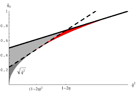
One therefore identifies three regions in the plane that are displayed with different colors in Fig. 2: (I) where the cutoff does not modify real emission (dark gray), (II) where the cutoff modifies the real emission (light gray), (III) where the presence of the cutoff inhibits completely real gluon emission (red).
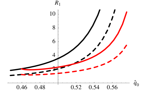
Explicit expressions for are reported in the Appendix A. We do not give those for which are relatively lengthy, but they can be found in the computer code. Fig. 3 shows the dependence of with and without the cutoff. Here and in all numerical examples of this section, we assume GeV, GeV. As anticipated, the structure function is unchanged for , and diverges less severely close to the endpoint. Therefore we do not perform any resummation, unlike [12, 13, 16].
A direct calculation of the virtual contributions in the presence of the cutoff is more cumbersome. However, since their expressions in the absence of the cutoff (on-shell scheme) are known from [15, 9], one can infer their expressions at arbitrary from the requirement that physical quantities be independent of the cutoff at each perturbative order when both power and perturbative corrections are consistently included. In particular, following the argument given in the previous section, we require the -independence of the integral over of each structure function:
| (9) |
In order to extract the -dependence of , we therefore consider the various sources of cutoff dependence in Eq. (9). The renormalization of the non-perturbative parameters and of is known to induce a cutoff-dependence of the form [8, 17]:
| (10) |
| (11) |
| (12) |
with111These expressions actually refer to the asymptotic value of , namely in the infinite limit. In general we employ a definition of and of the other OPE parameters at finite , but we actually choose to neglect terms in and in order to be consistent with Ref. [18] and with the way the global fit for the determination of these parameters is performed in [6]. This amounts to an ad-hoc perturbative redefinition of and .
| (13) |
It is worth recalling that the perturbative shifts in Eqs. (10-12) are not only conceptually, but also numerically quite important: using the current best experimental determination , for instance, we see that the perturbative shift amounts to almost 40% of that. We now write the perturbative contributions to the structure functions in the following way:
| (14) | |||||
| (15) |
where are the soft-virtual contributions in the on-shell scheme (without cutoff) calculated at [15] and [9] (see Appendix A).
The matching condition (9) is satisfied if and only if
| (16) |
where the range of the integral on the rhs is fixed by the decay kinematics. It is best performed numerically, while the are given by
| (17) |
The tree-level and power corrections contributions to the zeroth moments, and , can be found in Appendix B. The resulting factors read:
| (18) | |||
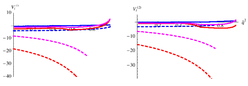
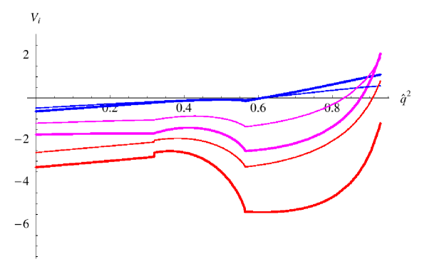
The complete virtual contributions to the three structure functions are shown in Fig. 4 for GeV, at and . There is a strong suppression of the virtual contributions with respect to the case without cutoff and the BLM corrections are typically smaller in relative terms, as it can be expected since the cutoff increases the typical gluon energy. It is worth noting that, following our discussion of Figs. 1-2, there are three regions of in the calculation of the integrals of in (16). This is illustrated in Fig. 5 for the case of the virtual contributions . For terms non-analytic in appear: the radius of convergence of the -expansion decreases for increasing and one does not expect the -independence to hold when one includes only a few higher dimensional operators, as done above. This is actually related to the poor convergence of the OPE at high that we will discuss more in detail later on. In practice, our choice of a cutoff close to 1 GeV implies a rather small value for the first threshold in . A high cutoff might indeed magnify at moderate the contribution of higher dimensional operators that are inevitably important in the high- tail. For this reason in our implementation we keep the complete -dependence of , but one can examine different options to study the theoretical uncertainty.
There is one point left to clarify in Eq. (4), namely the presence of a term. This is related to the difference that occurs between the kinetic mass of the b quark and the rest-energy that determines the kinematic end-point in the decay of the heavy quark [7]. This difference implies a finite perturbative shift of the endpoint, which manifests itself in Eq. (4) as a derivative of the Dirac delta. The values of can be calculated explicitly, but again we choose to infer their expressions from the -independence. To this end we require the cutoff-independence of the first moment (the only moment affected by the presence of a ). A procedure analogous to the one described for the virtual corrections yields:
| (19) | ||||
where the power corrections to the first central moments of the structure functions, , are given in the Appendix B. In the region , expanding in up to , we find
| (20) |
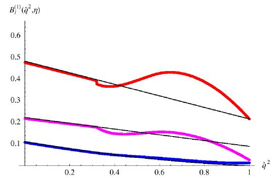
The are given as high precision approximate formulas that reproduce the numerical results within 1%.
As noted above, non-analyticity in is significant at high . This is again illustrated in Fig. 6 for the case of . The figure compares the full -dependence with the expansion in through . For there is no reason to expect to be well described by an expansion in . It turns out that non-analyticity is a minor effect for up to , while for it becomes relevant already at . On the other hand, is kinematically suppressed in the triple differential rate at high . In our practical implementation of perturbative corrections, we employ only the expanded formulas (20) for : the consequent mismatch at high manifests itself as a mild -dependence of the physical quantities that we compute and will be taken into account in our estimate of theoretical uncertainties.
3 Distribution functions in
The resummation of the leading twist effects in semileptonic decays close to threshold has been first studied long ago [19]. The structure functions are expressed as the convolution of their tree-level expressions with the light-cone distribution function whose support lies below , where is the meson mass:
| (21) |
where
is the light-cone component of the residual quark momentum, and is the distribution function. Eq. (21) is valid at the leading order in and does not include perturbative contributions.
The main properties of the distribution function in Eq. (21) are well-known: while it cannot be presently computed from first principles, its moments follow from the local OPE because they are related to the -moments of the structure functions . The distribution function is universal, i.e. independent of the considered structure function and shared by inclusive radiative and semileptonic decays. Moreover, since the leading-order moments of are independent of , the distribution function does not depend on .
Perturbative corrections can be included in the leading twist formula Eq. (21), by using in the convolution the short-distance perturbative structure functions that contain gluon bremsstrahlung and virtual corrections, instead of the tree-level .
The phenomenological and conceptual importance of subleading contributions to Eq. (21) has been repeatedly stressed in the last few years [7, 20]. In order to proceed beyond the leading order, we first of all modify Eq. (21) into
| (22) |
The advantage of the latter representation is that it automatically yields the correct hadronic endpoint for at arbitrary : since , the maximum value for is
| (23) |
Following [7] we do not split the distribution function into separate leading and subleading components. Rather, we define the finite- distribution function assuming the form of the convolution in Eq. (22) to hold at any order.
Clearly, such a distribution function is no longer universal: there must be a distribution function for each structure function and none of them corresponds exactly to the one describing the radiative decays. Similarly, since their moments including power corrections depend explicitly on , the distribution functions depend on . Finally, like the OPE parameters and the perturbative corrections, the distribution functions depend on the infrared cutoff : by construction, they are designed to absorb all infrared physics characterized by energy scales below . The form (22) of the convolution amounts to their perturbative definition.
We will therefore work with three distribution functions that, after including the perturbative corrections according to Eq. (22), must lead to -independent distributions. Thus, our generalized convolution reads
| (24) |
As mentioned already, all the available information on the distribution functions is encoded in their moments222The photon spectrum of is currently measured with a good accuracy at the factories for GeV. These data are important for the precise determination of and of the OPE parameters. However, the underlying distribution functions in semileptonic and radiative decays differ at the subleading level, and some of the subdominant effects do not seem to be under control [21]. Therefore, we believe that the photon spectrum in should not be used directly to determine the distribution function of semileptonic decays. On the other hand, as illustrated in [7] and its phenomenological applications, the photon spectrum can be accurately predicted, using our method, for not too high..
They can be extracted by matching with the OPE predictions for the -moments of the structure functions, known through and . Since the perturbative corrections to the Wilson coefficients of the power suppressed operators are not known, the moments of the can be determined neglecting perturbative corrections. We now consider the following moments of the structure functions
| (25) |
where we have left all -dependence implicit. We have also employed
| (26) |
and replaced with its lowest order term . The lhs of Eq. (25) is calculated including power corrections and reads
| (27) |
with the ’s given in the Appendix B, while the rhs becomes
| (28) |
where we have used the vanishing of all central moments of the tree-level structure functions for . is also given in App. B. The moments of the distribution functions are therefore given by
| (29) |
The functions are normalized to 1, up to small power corrections. The dependence of the first two moments is shown in Figs. 7.
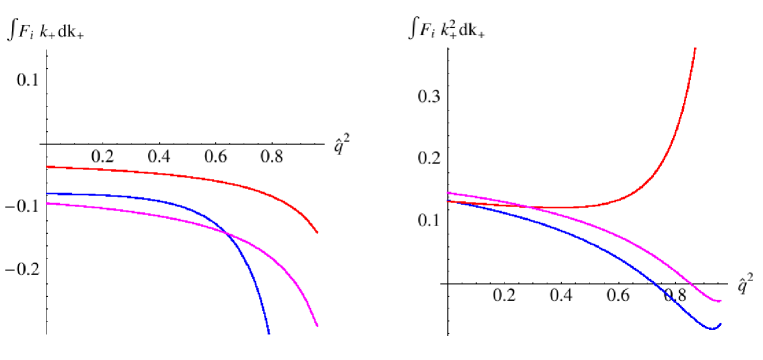
The importance of subleading contributions is apparent: the first moments for the three structure functions are quite apart from each other and we observe a strong -dependence at high , where they even diverge. The second moments of decrease with increasing and have a zero at . The variance of these two distribution functions decreases for growing , until it reaches negative values and the very concept of (positive definite) distribution function becomes meaningless. This is not surprising: as already noted in [19], the light-cone distribution function of the heavy quark cannot describe the semileptonic decay at high . We will come back to this subject in a dedicated section.
It is possible to use alternative forms of the convolution of the short and long-distance contributions, which differ at the subleading level from Eq. (24). For instance, one could use or instead of in the argument of . However, this would simultaneously redefine the power corrections to the moments of the light-cone function, and the consequent change in the distribution functions would largely compensate the change in the convolution at the level of observable structure functions. Therefore, adopting our procedure the choice of convolution is not an ad-hoc assumption.
Once the distribution functions are required to respect the OPE relations for their moments with power accuracy, the only element of arbitrariness concerns the ansatz that is employed for their functional form (see next Section). The latter is not specific to the treatment of the subleading-twist effects and is present already in the leading-twist analysis. Varying the functional form will allow us to estimate the associated theoretical uncertainty. The convolution (24) can now be used to compute the structure functions. It is useful to make the -function contained in explicit:
| (30) |
and write the detailed form of the convolution as
| (31) | ||||
Here we have employed .
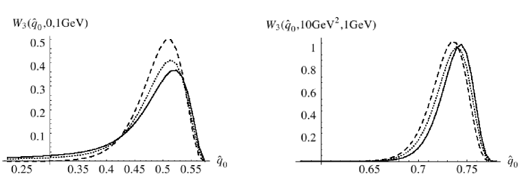
In Fig. 8 we show the -dependence of the convoluted at and for GeV for the exponential ansatz discussed in the next section. The plots compare the structure function calculated at the leading order (dashed curves) and at the next-to-leading order (dotted curves) in , and including also the corrections (solid curves). We observe that the width of the convoluted structure function shrinks significantly between and . The main effect of perturbative corrections at small is a broadening of the shape, due to real gluon emission. At higher , instead, real emission is progressively inhibited. In the example considered, lies just below (see Fig. 2). Therefore the only appreciable perturbative effect is a shift of the peak somewhat towards higher values, and is driven by the term in Eq. (4). The structure functions behave in a very similar way.
4 Functional forms
We have seen that only the first few moments of the distribution functions are known. They are given in terms of matrix elements of local operators that are measured in semileptonic and radiative decays. The modelling of QCD dynamics in the threshold region therefore requires an ansatz for the functional form, which must comply with the constraints coming from the first few moments. Several functional forms have been proposed in the literature. They have to be exponentially suppressed at large negative and to vanish at the endpoint . We will further assume the positivity of . As suggested by its probabilistic interpretation, the primordial should be positive definite, but radiative corrections can potentially change its sign, in analogy with the parton distribution functions of deep inelastic scattering. In our approach with the Wilson cutoff effects of this kind are excluded in the negative tail and we choose to neglect them altogether, assuming positive distribution functions.
The basic two-parameter functional forms proposed in the literature [22, 13, 7] are
| (32) | |||||
| (33) | |||||
| (34) | |||||
| (35) |
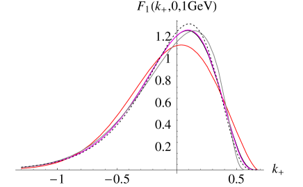
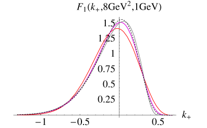
The parameters are fixed by the first two normalized moments of and can be easily found numerically. A comparison of the resulting distribution functions at and GeV2 is shown in Fig. 9. The numerical inputs for the moments are taken from [6]. The results for the other two light-cone functions are very similar. The hyperbolic and exponential forms are almost indistinguishable in the plot. Indeed, once the first two moments are fixed, the shape of the various curves is determined to a large extent by the properties of the tails. In this respect, there is not a large variety in (32)-(35). It is not difficult to find alternatives: for instance, one could modify the exponential form as in
| (36) |
which is also displayed in Fig. 9 (dashed curve) and is characterized by a higher negative tail.
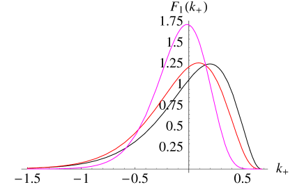
It is interesting to see the effect of subleading corrections to the moments of the distribution functions: this is illustrated in Fig. 10, where is computed using the exponential ansatz retaining only the leading contributions to its moments, and including all the known power corrections.
The need for more flexibility in the choice of the functional form can also be understood by comparing the third normalized moments of the curves displayed in Fig. 9. For a given value of , they are remarkably close to each other. Let’s consider : while the gaussian form yields for the third normalized moment, exponential, hyperbolic, and roman forms cluster around , and that in (36) yields . On the other hand, the OPE predicts the third moment to be , up to unknown and corrections. Using the results of the fit in [6], this amounts to , in rough agreement with the values mentioned above. The situation does not change significantly with , but the spread between different forms decreases further.
Clearly, a mismatch between the third moment of the two-parameter forms we have considered and the OPE prediction might signal either large and possibly -dependent subleading contributions to the OPE, or that the specific functional forms are disfavored by present data on inclusive semileptonic moments. A line is difficult to draw, but none of the basic forms in (32–36) appears particularly disfavored. Rather than using the third moment to constrain the distribution functions, we have used it to gauge the diversity in the functional forms we employ.
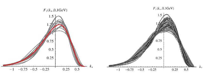
A straightforward generalization of the above basic forms consists in multiplying them by a distortion factor that can be a polynomial, positive in the domain, or a more general positive function. In principle the distortion can depend on . Of course not all the distortions yield acceptable solutions. In particular, we discard shapes with two or more maxima, but keep those with an inflection point. We are particularly interested in distortion factors that modify the third moment. This can happen when the distortion enhances or suppresses the lower (negative ) tail, or, to a lesser extent, with an asymmetric and bounded function, like a constant with a sinusoidal perturbation. In general it is difficult to find distortions that modify significantly the third moment. A representative but not exhaustive sample of distribution functions , based on the exponential form and complying with the first and second moment constraints, is shown in Fig. 11. All the functions in the sample satisfy the first two moment constraints and yield third moments that differ by less than 30% from the basic exponential form. Since there is no reason of principle to discard any of them, they will be used, together with similar ones, in our study of the theoretical uncertainty. Changing also the basic functional form one gets the plot on the rhs of Fig. 11, with almost a hundred different forms.
5 The high- tail
We have seen that the formalism developed in Sec. 3 cannot be applied at high . The relevance of Fermi motion subsides at high and Fig. 7 shows that the variance of the distribution functions becomes negative at -0.8, as a consequence of effects. While the leading contributions to the -th central moment of the structure function , , is suppressed by at large , subleading contributions in have a weaker suppression that enhances their weight at high .
We also recall that our discussion of perturbative corrections points to larger uncertainties in the high region. We have seen in Sec. 2 that the expressions for the perturbative corrections become non-analytic in for . This is a manifestation of the same problem mentioned above: at high the contribution of higher dimensional operators is no longer suppressed.
A simple way to visualize the problem is to plot the width of the physical range in as a function of , as in Fig. 12. The OPE structure functions are smeared over a region in of width .
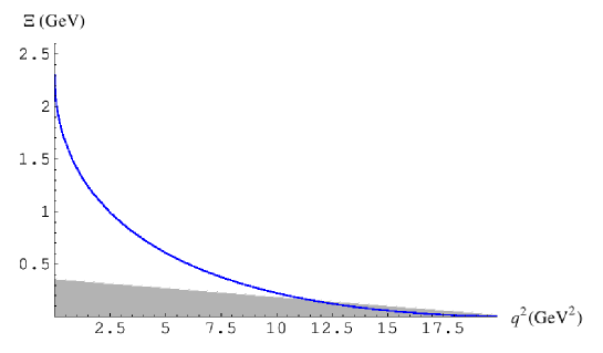
shrinks rapidly with , reaching a size comparable to for . The range can also be compared with the typical width of the structure function, which at the leading order in is GeV. As shown in Fig. 12, they are equal for and for higher the width of the physical -range is smaller than the width of the structure functions, a situation that makes all local OPE results unreliable.
It is indeed well-known that for very large the local OPE fails to provide a reliable description of the semileptonic decay, as the dynamics in that region is not characterized by a short-distance scale [19, 23]. The Wilson coefficients in the power expansion, for instance, grow like . The origin of this enhancement at high can be understood by calculating the -differential rate as the integral over of the double differential rate,
| (37) |
It is related to the presence of the square root, a non-analytic term that follows from the kinematic constraints on the electron energy — the first -function in Eq. (1). Expanding the square root in around the endpoint one gets
| (38) |
Clearly, the convergence radius of the series gets smaller at higher and, in particular, higher orders become more and more important. Replacing the square root in (37) with its expansion (38) and integrating over one sees that non-perturbative contributions are organized in the series
| (39) |
and one can verify that unknown corrections become comparable to corrections at .
Since the contributions of higher dimensional operators become more and more singular at high , we see from (39) that their contribution to the total width is singular for . In particular, the Darwin operator contribution to the differential rate is ()
| (40) |
which upon integration over leads to a logarithmic singularity that can be regulated by the quark mass [10, 24]. This unphysical singularity is removed by a one-loop penguin diagram that mixes at the Weak Annihilation four-quark operator into the Darwin operator. The cancellation is discussed in detail in [25]. Defining
| (41) |
one finds that the sum of the contributions of the WA and Darwin operators to the semileptonic total width is
| (42) |
which is free of singularities. The scale is the renormalization scale of the WA operator. The constant accompanying the logarithm in Eq. (42) depends on the renormalization scheme; we have employed here the same scheme as in Ref. [25]. At the level of the differential spectrum of Eq. (40), the singularity is replaced by and is accompanied by a term whose coefficient contains and can be read off directly from Eq. (42).
It is well-known that in the factorization approximation the matrix element vanishes, and that WA is phenomenologically important only to the extent factorization is actually violated. Since Eq. (42) is independent of the scale , up to corrections that we neglect, we have in the scheme . Clearly factorization may hold only for a certain value and, therefore, if factorization holds at , namely , a change of the scale provides a rough measure of the (minimal) violation of factorization induced perturbatively.
We should stress that the inclusion of WA removes the unphysical singularity in the OPE but not its intrinsic limitations at high . The local OPE non-perturbative contributions for the rate with arbitrary cuts on , , and is reported in Appendix C. It includes WA contributions as discussed above. The main spectra follow from these expressions upon differentiation. It can be easily seen that both the rate and some of the differential spectra become negative for a sufficiently high cut on , a clear sign of the importance of higher dimensional operators. This is apparent in the case of Eq. (40) where the singularity drives the spectrum to negative values for , see Fig. 13.333This is by far the dominant but not the only negative contribution. Even in the absence of the Darwin term the differential rate becomes negative at very high .
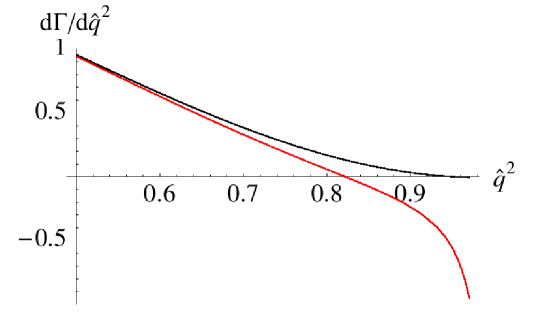
Because of the limitations of the OPE in the high region, it is preferable to model the tail in a way that is both compatible with the positivity of the spectra and incorporates some features of the OPE. We want to modify the OPE expressions before the differential rate becomes negative. To this end we change approach for greater than a certain and adopt one of the two following methods.
The first method is based on the local OPE result without the convolution with the light-cone distribution functions. One starts from the OPE distribution (40) and introduces a damping factor in the singularity
| (43) |
that maintains the differential rate positive for appropriate values of (see Fig. 13). We have also explicitly written the Dirac delta at the endpoint. The damping factor can also be applied to the and differential distributions. In a realistic setting one could expect a smooth (positive) bump close to maximal . However, since in the following we will always integrate over the tail, the rough modelling of (43) is sufficient. It should be clear that positivity of the rate implies . The dimensionless parameter is related to the WA matrix element and to the WA scale by integrating over .444 The relation is . In the case of our default choice , the minimum value corresponds to or equivalently to a factorization scale for WA . The amount of WA implied by this ansatz for the high- tail grows with : corresponds, in the default setting, to (). Conversely, the experimental determination of would allow us to fix the value of .
Since we will mainly be interested in integrated quantities (for instance total rates with cuts), this approach is based directly on the formulas in App. C and does not provide a triple differential distribution in the high region, but includes the endpoint effect parameterized by . Perturbative corrections are implemented as for but again there is no convolution. We adopt this first method as our default choice.
In the second method that we employ to model the high region we freeze the distribution functions at and use it in the convolution formula for all . Because of the decreasing phase space available at higher , this approach effectively amounts to gradually phasing all power-corrections out. Although WA does not explicitly enter in this case, the ansatz corresponds to a certain amount of WA depending on the value of and on the precise values of the other heavy quark parameters. For instance, for and the default values of the non-perturbative parameters, it corresponds to (). An additional amount of WA can be easily accommodated in this framework as an extra contribution at the -endpoint. The triple differential rate here is available for each point in the phase space.
While there is no doubt that the local OPE expansion fails at high , the precise determination of its range of applicability is an open question. We employ the formulation based on the convolution of Eq. (31) for with
| (44) |
keeping the maximum value of lower than the value for which the variance of one of the distribution functions gets negative, , because of numerical instabilities in dealing with very narrow light-cone functions. To model the high- tail at we employ one of the two methods described above. The difference of the two approaches, as well as a variation of the parameters in Eqs. (42,43,44) provide us with an estimate of the theory uncertainty in the high region.
6 Results and theoretical errors
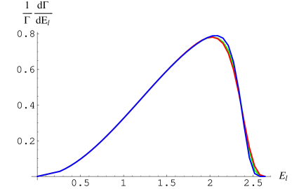
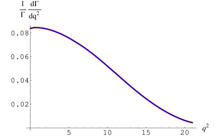
Let us now illustrate our method with a few applications. We start by showing the main physical distributions following our default approach, based on Eq. (31) for , and on the local OPE modified as in (43) for higher . We employ the central values of the fit in [6] for the non-perturbative parameters at , namely
and set and in Eq. (43). All numerical results in this section are obtained with a C++ implementation of the procedure described in the previous sections.
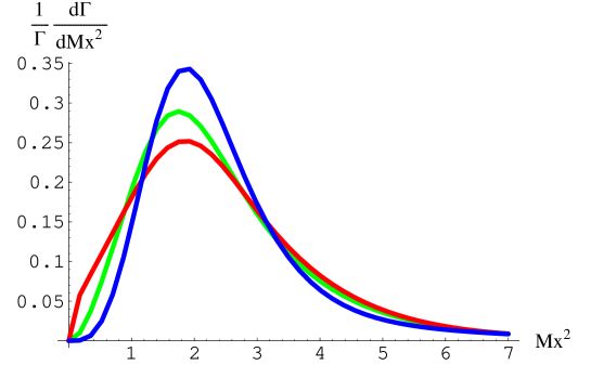
Fig. 14 shows the electron energy and spectra using a few different functional forms. Since we impose the local OPE constraints on the distribution functions at fixed , the spectrum is by construction independent of the adopted functional form, while the lepton energy spectrum shows a limited dependence. The hadronic invariant mass spectrum is displayed in Fig. 15. In this case the difference between functional forms is more pronounced.
One of the checks we have performed concerns the total width that in our scheme is given by
| (45) | |||||
where , , and we have left the -dependence of implicit. The first parenthesis contains the dominant short distance electroweak correction [26] which amounts to about 1.4%. The perturbative QCD corrections in (45) have been known for a while (see [9] for a complete list of references). The non-BLM contributions to the total rate are also known [27] and amount to about +0.5% in our scheme, however we do not report them in (45) as they are absent in our triple differential rate. The total semileptonic decay rate can also be obtained by integrating the triple differential distribution computed in our default setting with the modified high- tail. In this case the result is about 1.4% higher than Eq. (45), using the same input values. This small difference is related to the perturbative corrections at the -endpoint and might in principle be accounted for by a more accurate treatment of the WA contribution, but it will be added to theoretical error budget. Using the second option discussed at the end of the previous section, namely freezing the distribution functions without taking into account any extra effect at the endpoint, the total rate differs from (45) with default values by .
The next application we consider is the extraction of from some of the latest experimental results. We consider the following experimental results:
This list is far from being complete and it is meant for the purpose of illustration only. The analysis B was proposed in [31] and suffers most from the high- uncertainty discussed in the previous section (see also Ref. [32]), but in all three cases the high region is probed. In comparing with experiment we avoid averaging the various experimental results. In the case B, however, we take the arithmetic mean of the two experimental central values as reference value. The partial rate given by the experiments is compared with our theoretical predictions, yielding the values for listed in Table 1:
| (46) |
| cuts | exp | par | pert | tail model | ff | tot th | ||||
| A [28] | 3.87 | 0.71 | 6.7 | 3.5 | 1.7 | 1.6 | 2.0 | |||
| B [28, 29] | 4.44 | 0.38 | 7.3 | 3.5 | 2.6 | 3.0 | 4.0 | |||
| C [30] | 4.05 | 0.30 | 5.7 | 4.2 | 3.3 | 1.8 | 0.9 |
The central values given in Table 1 refer to our default setting, with an exponential ansatz for the distribution functions. The total theoretical errors in the last column of Table 1 are obtained by combining all theory errors in quadrature, with the exception of the asymmetric errors due to the functional forms and to (see below), which are added linearly and kept asymmetric.
We now consider the uncertainty of our theoretical predictions for Table 1. There are both parametric uncertainties for instance due to the OPE parameters (, , etc.) and intrinsic uncertainties, related to various limitations of our approach. We identify the following sources of uncertainty:
-
1.
the value of , and of the other non-perturbative parameters;
-
2.
higher order perturbative and non-perturbative corrections;
-
3.
the functional form of the distribution functions;
-
4.
WA and the high- tail.
For what concerns the parametric errors (par), we employ and take the values of the non-perturbative parameters from the fit [6] including all correlations. Not surprisingly, the by far dominant parametric error is related to the uncertainty in the quark mass. The value of extracted is quite sensitive to the precise value of the quark mass. For instance, if one employs , as suggested by a fit to charmed semileptonic only, instead of , the central values in Table 1 change to in the A,B,C cases, respectively..
To estimate higher order perturbative corrections we change the hard cutoff in the range and rescale the discrepancy in the total rate due to perturbative effects in the highest region to the fraction of events. We also consider the overall size of the corrections in our analysis (% in the A,B,C cases, respectively). We take as overall perturbative error in each case the maximum between 40% of the corrections and the uncertainty obtained by combining the above and errors. To estimate higher order non-perturbative corrections and missing perturbative corrections to the Wilson coefficients of power-suppressed operators, we vary the non-perturbative parameters within 30% of their central values in an uncorrelated way. This leads to errors that are negligible in comparison with those in Table 1.
The uncertainty due to the functional form (ff) of the distribution functions is estimated by comparing a total of about 30 different forms. We display in Table 1 the maximal positive and negative variations wrt to the default exponential ansatz. In all cases it amounts to a relatively small error.
Concerning the high- tail we consider three related sources of uncertainty: the modelling of the tail, the arbitrariness in the choice of the scale where the modelling sets it, and the WA matrix element. We estimate the error on modelling the tail by comparing our default approach with the second method outlined at the end of the previous section, by varying the parameter in (43) and change between 8.5 and .
In connection to WA we observe that all we presently know about is that it is not unexpectedly large because no significant excess was found in the high- region by CLEO [33]. In the context of our model of the high- tail, this experimental result can actually be approximately translated into an upper bound on , which in turn is related to or . The CLEO bound is not very strong, at 90%CL, and still falls short of the expected size for the WA contribution to the total rate [34]. We vary in the conservative range . In terms of model-independent parameters this corresponds to . In the future, it will be possible to measure the size of the WA expectation values using, for instance, measurements of the spectrum close to the endpoint and of its moments [25], and by comparing the semileptonic rates of and .
In our default set-up we have assumed , but while we expect it to be positive and possibly small, there is no compelling reason for it to vanish. The error in Table 1 should therefore not be treated as gaussian. It is worth observing that a non-zero value for would bring the different experimental determinations of closer to each other. For instance, would lead to in the A,B,C cases, respectively. Suggestive as this may sound, it is clear from our analysis that an upper experimental cut on would improve the theoretical precision in the inclusive determination of . In the absence of a dedicated experimental analysis, we can subtract Belle’s results for the cases A and B [28] and extract a value of for the combined cut , , and , i.e. with an upper cut on . The cut on is relatively low and the predicted fraction of events in this case is only 33%, but the measured rate is lower than expected: it corresponds to with % theoretical error, dominated by parametric uncertainties. We were unable to compute the experimental uncertainty for the case, which will certainly be larger than those in Table 1. Such a low value of may, however, indicate either an experimental problem or an underestimate of theoretical errors in the high region, which is common to the three cases considered in Table 1.
7 Conclusions
We have calculated the triple differential distribution for inclusive semileptonic decays without charm, , consistently including all the known perturbative and non-perturbative effects, through and , respectively. Our theoretical framework is based on the OPE and incorporates a hard Wilson cutoff . This involved new perturbative calculations discussed in Section 2.
Our approach has several new elements that we have listed in the Introduction and explained in detail throughout the paper. We recall the main ones: we parameterize the Fermi motion in terms of a single light-cone function for each structure function and for any value of , and include consistently the subleading effects; this is accomplished at the same level of model-dependence as for the leading twist distributions; we implement for the first time the complete BLM corrections to the triple differential rate; we present a detailed discussion of the high- tail and of Weak Annihilation effects. Our approach is completely implemented in a C++ code that is available from the authors.
We have extracted from some of the latest and most precise experimental data, providing a detailed estimate of the theoretical uncertainty. Our results, listed in Table 1, agree within theoretical errors with those obtained with other methods used by HFAG [12, 13]. We find that the dependence on the functional form assumed for the distribution functions is rather weak. However, the critical role played by the high- tail becomes evident from our analysis; it contributes in a significant way to the theoretical uncertainty of the present inclusive determinations of . We have modeled the high- region in two different ways complying with the positivity of the differential spectra and have accounted for the WA contributions. We find that non-vanishing WA effects tend to suppress the value of extracted from the data and, using recent Belle results, we have argued that the low- sample of events leads to a lower value of that conflicts with that extracted from the sample.
Since the high- tail presently leads to a sizeable uncertainty, we encourage our experimental colleagues to pursue analyses with an upper cut on , and to perform an accurate separate measurement of this domain.
Acknowledgements
P. Gambino is grateful to Einan Gardi for clarifying discussions. N. Uraltsev thanks I. Bigi for discussions and collaboration on related issues and the Department of Theoretical Physics of the University of Turin for hospitality during part of the work. This work was supported in part by the NSF grant PHY-0355098, by MIUR under contract 2004021808-009, and by a European Community’s Marie-Curie Research Training Network under contract MRTN-CT-2006-035505 ‘Tools and Precision Calculations for Physics Discoveries at Colliders’.
Appendices
Appendix A Perturbative corrections
In this Appendix we provide all necessary analytic expressions for the perturbative corrections to the three structure functions in the scheme with a hard cutoff . In the absence of cutoff the real gluon emission terms can be gleaned from [15, 9]:
| (47) |
| (48) | ||||
| (49) |
where and
| (50) |
The plus distributions in Eqs. (A–49) are defined by ()
| (51) |
where is a smooth function.
The NLO real emission contributions to the structure functions in the presence of a Wilsonian cutoff, see (7), are a new result and read as follows:
| (52) |
| (53) |
| (54) |
Appendix B Structure functions in the local OPE and their
-moments
In the adopted normalization, the power corrections to the structure functions read
| (58) |
| (59) |
| (60) |
We have used the short-hand notation , where the -th derivative of the Dirac delta is taken wrt its argument. We give explicit expressions for the zeroth, first and second -moments, at fixed , of the three form factors, up to corrections in the OPE. Separating the tree-level and power corrections contributions, we define
| (61) |
and
| (62) |
The functions ’s defined in Sec. 3 correspond to central moments and are linear combinations of above or moments:
| (63) |
The explicit expressions for the zeroth moments are:
| (64) |
| (65) |
The explicit expressions for the first moments are:
The explicit expressions for the second moments are:
| (66) |
Appendix C Local OPE results with arbitrary cuts
In this Appendix we report the local OPE results for the rate of subject to standard cuts on , , and . The expressions contain only the non-perturbative power corrections. We adopt the following notation
| (67) |
where and are lower cuts on , and is an upper cut on the invariant mass of the hadronic system. Only , the effective lower cut on , is relevant for power corrections: the upper cut on the hadronic mass must be lower than to play a role in the following expressions. There is also a relation between and : both cuts are relevant only when , otherwise only is relevant. The total width subject to the above cut is given in the two regions by
| (68) | |||||
and
| (69) | |||||
References
- [1] UTFit Collaboration, M. Bona et al., JHEP 10, 081 (2006), hep-ph/0606167, and http://utfit.roma1.infn.it for the Winter 2007 update. See also CKMfitter Coll., http://ckmfitter.in2p3.fr.
- [2] J.M. Flynn and J. Nieves, arXiv:0705.3553v1 [hep-ph].
- [3] P. Ball, arXiv:0705.2290v1 [hep-ph].
- [4] I. Bigi, N. Uraltsev and A. Vainshtein, Phys. Lett. B293 (1992) 430 and Phys. Rev. Lett. 71 (1993) 496; B. Blok, L. Koyrakh, M. Shifman and A. Vainshtein, Phys. Rev. D49 (1994) 3356; A. V. Manohar and M. B. Wise, Phys. Rev. D 49 (1994) 1310.
- [5] B. Aubert et al. [BABAR Coll.], Phys. Rev. Lett. 93 (2004) 011803 [hep-ex/0404017]; C. W. Bauer et al., Phys. Rev. D 70 (2004) 094017 [hep-ph/0408002] v3;
- [6] O. Buchmuller and H. Flacher, Phys. Rev. D 73 (2006) 073008 [arXiv:hep-ph/0507253] and 2007 update http://www.slac.stanford.edu/xorg/hfag/ semi/LP07/gbl_fits/kinetic/lp07-update.pdf
- [7] D. Benson, I. I. Bigi and N. Uraltsev, Nucl. Phys. B 710 (2005) 371 [arXiv:hep-ph/0410080].
- [8] I. I. Y. Bigi, M. A. Shifman, N. Uraltsev and A. I. Vainshtein, Phys. Rev. D 56 (1997) 4017 [arXiv:hep-ph/9704245] and Phys. Rev. D 52 (1995) 196 [arXiv:hep-ph/9405410].
- [9] P. Gambino, E. Gardi and G. Ridolfi, JHEP 0612 (2006) 036 [arXiv:hep-ph/0610140].
- [10] M. Gremm and A. Kapustin, Phys. Rev. D55 (1997) 6924.
- [11] Heavy Flavour Averaging Group (HFAG), E. Barberio et al., arXiv:0704.3575v1 [hep-ex], http://www.slac.stanford.edu/xorg/hfag/
- [12] J. R. Andersen and E. Gardi, JHEP 0601 (2006) 097 [arXiv:hep-ph/0509360] and JHEP 0506 (2005) 030 [arXiv:hep-ph/0502159]; E. Gardi, arXiv:hep-ph/0703036.
- [13] B. O. Lange, M. Neubert and G. Paz, Phys. Rev. D 72 (2005) 073006 [arXiv:hep-ph/0504071].
- [14] V. Aquila, P. Gambino, G. Ridolfi and N. Uraltsev, Nucl. Phys. B 719 (2005) 77 [arXiv:hep-ph/0503083].
- [15] F. De Fazio and M. Neubert, JHEP 9906, 017 (1999) [arXiv:hep-ph/9905351].
- [16] U. Aglietti, G. Ferrera and G. Ricciardi, Nucl. Phys. B 768 (2007) 85 [arXiv:hep-ph/0608047]; A. K. Leibovich, I. Low and I. Z. Rothstein, Phys. Lett. B 486 (2000) 86 [arXiv:hep-ph/0005124].
- [17] D. Benson, I. I. Bigi, T. Mannel and N. Uraltsev, Nucl. Phys. B 665 (2003) 367 [arXiv:hep-ph/0302262].
- [18] P. Gambino and N. Uraltsev, Eur. Phys. J. C 34 (2004) 181 [arXiv:hep-ph/0401063].
- [19] I. I. Y. Bigi, M. A. Shifman, N. G. Uraltsev and A. I. Vainshtein, Int. J. Mod. Phys. A 9 (1994) 2467 [arXiv:hep-ph/9312359].
- [20] A. K. Leibovich, Z. Ligeti and M. B. Wise, Phys. Lett. B 539 (2002) 242 [arXiv:hep-ph/0205148]; C. W. Bauer, M. Luke and T. Mannel, Phys. Lett. B 543 (2002) 261 [arXiv:hep-ph/0205150]; S. W. Bosch, M. Neubert and G. Paz, JHEP 0411 (2004) 073 [arXiv:hep-ph/0409115].
- [21] S. J. Lee, M. Neubert and G. Paz, Phys. Rev. D 75 (2007) 114005 [arXiv:hep-ph/0609224].
- [22] R. D. Dikeman, M. A. Shifman and N. G. Uraltsev, Int. J. Mod. Phys. A 11 (1996) 571 [arXiv:hep-ph/9505397].
- [23] I. I. Y. Bigi and N. G. Uraltsev, Nucl. Phys. B 423 (1994) 33 [arXiv:hep-ph/9310285].
- [24] B. Blok, R. D. Dikeman and M. A. Shifman, Phys. Rev. D 51 (1995) 6167 [arXiv:hep-ph/9410293].
- [25] P. Gambino, G. Ossola, N. G. Uraltsev, JHEP 0905 (2005) 010 [hep-ph/0505091].
- [26] A. Sirlin, Nucl. Phys. B 196 (1982) 83.
- [27] T. van Ritbergen, Phys. Lett. B 454 (1999) 353 [arXiv:hep-ph/9903226].
- [28] I. Bizjak et al. [Belle Collaboration], Phys. Rev. Lett. 95 (2005) 241801 [arXiv:hep-ex/0505088].
- [29] B. Aubert et al. [BABAR Collaboration], Phys. Rev. D 73 (2006) 012006 [arXiv:hep-ex/0509040].
- [30] B. Aubert et al. [BABAR Collaboration], arXiv:hep-ex/0507017.
- [31] C. W. Bauer, Z. Ligeti and M. E. Luke, Phys. Rev. D 64 (2001) 113004 [arXiv:hep-ph/0107074].
- [32] I. Bigi and N. Uraltsev, Int. J. Mod. Phys. A 17 (2002) 4709 [arXiv:hep-ph/0202175].
- [33] J.L. Rosner et al. [Cleo Collaboration], hep-ex/0601027.
- [34] N. Uraltsev, Int. J. Mod. Phys. A 14 (1999) 4641 [arXiv:hep-ph/9905520].