Visualization, Exploration and Data Analysis of Complex Astrophysical Data
Abstract
In this paper we show how advanced visualization tools can help the researcher in investigating and extracting information from data. The focus is on VisIVO, a novel open source graphics application, which blends high performance multidimensional visualization techniques and up-to-date technologies to cooperate with other applications and to access remote, distributed data archives. VisIVO supports the standards defined by the International Virtual Observatory Alliance in order to make it interoperable with VO data repositories. The paper describes the basic technical details and features of the software and it dedicates a large section to show how VisIVO can be used in several scientific cases.
1 Introduction
The astronomical community has always dedicated special attention to the growth of graphical and visualization tools, driving their evolution or even being directly involved in the development of many of them.
At present, the most popular software for astronomers can be subdivided into two main categories: tools for image display and processing and tools for plotting data. Notable among the former are IRAF, by NOAO; ESO-MIDAS, by the European Southern Observatory; SaoImage, by the Smithsonian Astrophysical Observatory and GAIA, by ESO. Many other tools are available, but we refer to dedicated surveys for a complete list. Gnuplot and SuperMongo are popular applications adopted for 2D data plots. A more sophisticated solution is represented by IDL, by ITT Visual Information, which is characterized by a large library of functions specifically developed for astrophysics. Again, for a complete list, we refer to specific surveys.
Among the most popular N-body visualization codes used by the community there are: TIPSY, motivated by the need to quickly display and analyze the results of N-body simulations, it is mainly limited to this type of data; ParaView, produced by Kitware in conjunction with the Advanced Computing Laboratory at Los Alamos National Laboratory (LANL), the goal of the project is to develop scalable parallel processing tools with an emphasis on distributed memory implementations; IDL, mentioned above, contains support for N-body data display, but is not free software.
A new generation of graphic software tools is now emerging. These tools are designed to overcome the limits and the barriers of traditional software by exploiting the latest technological opportunities. The main challenges and objectives are the following:
-
•
High performance and multi threading, in order to exploit multi-core systems, large memories and powerful graphic cards and co-processors. This allows the user to handle large amount of data in real-time.
-
•
Interoperability, allowing different applications, each specialized in doing different things, to interact with each other in a coordinated and effective way according to well-defined protocols. The aim is to provide to the user a complete suite of tools to best analyze his/her data. Huge, monolithic and often inefficient tools are obsolete.
-
•
Collaborative work. The tools allow several users to work on the same data at the same time from different places, exchanging experience, information and expertise.
-
•
Access to distributed resources, via web services and/or Grid protocols. Often, data can no longer be moved from data centres as it is too large and complex. The astronomer must have the tools to access it, independently of his geographical location in a fast and reliable way.
Tools like VisIVO, Aladin (Bonnarel, 2000) and Topcat (Topcat, ), have been recently developed in the framework of the Virtual Observatory (www.ivoa.net) to achieve all or some of these goals. In this paper we will focus in particular on VisIVO, which stands for Visualization Interface for the Virtual Observatory. VisIVO is being developed as a collaboration between the Italian National Institute for Astrophysiscs (INAF) - Astrophysical Observatory of Catania and CINECA (the largest italian academic high performance computing centre) in the framework of the FP6 EU funded VO-Tech project. The next section gives a short review of the basic functionality of VisIVO, while section 3 describes PLASTIC, a messaging protocol which allows heterogeneous applications to work together. Part of section 3 and section 4 are dedicated to presenting several scientific cases in which the support of graphics and visualization is of primary importance. In these sections we show some of VisIVO’s capabilities in action, demonstrating how they can be effectively used in practical applications.
2 VisIVO
VisIVO is a C++ application specifically designed to deal with multidimensional data. It is free software available both for MS Windows and for GNU/Linux (porting to MacOS is in progress). It can be downloaded from the web site http://visivo.cineca.it. The software is built on the top of the Multimod Application Framework (MAF)(Viceconti, 2004). MAF is an open source framework for the development of data visualization and analysis applications. It provides high level components that can be easily combined to develop a vertical application. It is being developed by the visualization group of CINECA and it can be downloaded from the web site http://openmaf.cineca.it. The framework is based on the Visualization ToolKit (VTK) (Schroeder, 2004) library for the multidimensional visualization and on the wxWidgets library, a portable Open Source GUI library, for the user interface. It incorporates other open libraries, (for example for data encryption) or drivers for virtual reality devices (3D mouse, gloves, haptics etc.). VisIVO’s architecture strictly reflects the structure of a typical scientific application built with the MAF, being mainly developed in the highest layers of the framework. The software exploits, wherever possible, the standard visualization services, views, operations and interface structures provided by the framework and implements all the elements that are specific to the visualization and analysis of astronomical data.
Extensions to the basic MAF infrastructure have been developed in order to match astronomy-specific requirements and to provide the highest performance. Internal data representation is in the form of a Table Data structure, which is composed of a sequence of variables loaded from a data source such as a file or a database. Regardless their original type, variables are all converted to double format. While this incurs a penalty in the application’s memory needs, it provides the necessary precision in some of the data processing stages. Once a table is loaded the user can manage and visualize the data. These operations do not increase the memory usage as long as they do not create new tables or new fields: the visualization process is carried out using references to the Table Data with no data replication. In order to visualize data, the user has to set which of the loaded fields will be used as the coordinate system of a Cartesian reference frame. In this way, the software ensures maximum flexibility in data usage.
2.1 VisIVO for data visualization
Data visualization is the main target of VisIVO. The software is designed to simultaneously handle as many properties as possible. Complex tables can be loaded and manipulated, new fields can be derived and finally represented graphically, using points, colours, transparencies, surfaces, glyphs and volume rendering. The first step of a working session is usually data loading. Data can be read from files; VisIVO supports different kinds of file formats: standard file formats, like VOTables, FITS, HDF5, ASCII, raw binaries and the native data format of the popular simulation code (Springel, 2000). The VOTable format is an XML standard for the interchange of astronomical data, defined by the International Virtual Observatory Alliance (IVOA, http://www.ivoa.net). Data is represented as a set of tables, each table being an unordered set of rows, whose format is specified in the table XML metadata. Rows are sequences of table cells, each containing either a primitive data type or an array of such primitives. VOTables can also contain links to external files as a separate data source. VisIVO uses the Savot VOTable parser developed by CDS111Centre de Donnes astronomiques de Strasbourg to load and write VOTables. FITS and HDF5 importers are implemented using the published API and libraries. The ASCII table format consists of columns of data spaced with the most common separation characters (space, tab etc.). Raw files are sequences of variables written as binary dumps of the memory. The binary files can be managed by descriptor files which store the associated information (number of variables, data types etc.). VisIVO can also interact with CDS VizieR data service (Ochsenbein, 2000), retrieving data directly from remote archives (see par. 2.3).
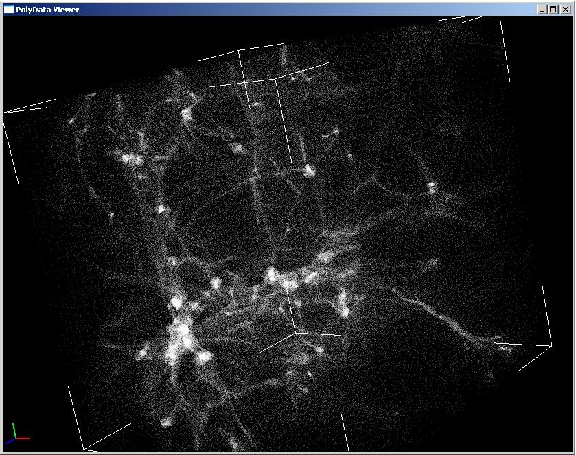
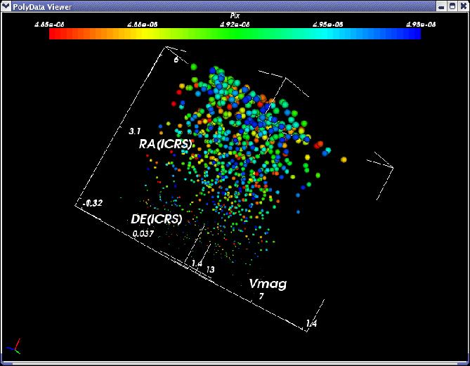
Once data is loaded it can be visualized and analyzed. VisIVO can deal with both structured and unstructured data. The former is represented by fields defined on a regular mesh. The latter is data with no special geometry; it is treated as sets of points. Graphically, unstructured data have a default representation as pixels. The points geometrical distribution is set by selecting three of the fields loaded as Table Data. For example: the , , coordinates of the particles from a N-Body simulation, or the RA (Right Ascension) - DE (Declination) - Vmag (Johnson magnitude V) fields for data from stellar catalogues (figure 1).
Besides their geometric position, points can be used to display further quantities, using colours and glyphs (3D shapes, like spheres or cubes). Points can be coloured as a function of a given scalar field (e.g. their temperature or their spectral index) with a colourmap that the user can customize. Each point can also have an associated glyph, whose size can be a function of one (for spheres) or two (for cubes, cylinders, pyramids) fields. A vector quantity can be visualized as well, using either oriented segments or arrows. Vectors can also be coloured according to their magnitude.
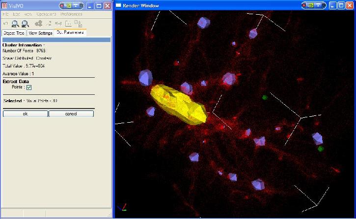
If the data size is too large to be managed in memory, VisIVO allows the user also to extract a random subset of points. It is also possible to select the points which lie in a region the user is specifically interested in (e.g a galaxy cluster in a cosmological simulation, or a globular cluster in a catalogue of stars). The selection can be accomplished using either a rectangular sampler or the cluster finder utilities. For the latter, the following cluster identification method is implemented. A field associated to the points (e.g. the point mass) is used to set a threshold. All the points that have a value of the field above the threshold, comprise a cluster. Surfaces which divide regions above and below the threshold can be visualized (see figure 2). Regions geometrically disjoint (i.e. their threshold surfaces do not overlap) are identified as separate clusters.
Structured mesh-based data do not have a default graphical representation. VisIVO can visualize them using volume rendering and isosurface. Volume rendering is a visualization technique in which the field values are represented by different colours and different transparencies. The global effect is a cloud appearance. This method enables the user to emphasize also the inner parts of the volume. Isosurfaces are surfaces of given value calculated from a mesh-based quantity. The isosurface can be defined as the surface which divides regions in which a given field has value above a certain value from regions in which it is below that value.
2.2 VisIVO for data analysis
VisIVO provides various built-in utilities that allow the user to perform
mathematical operations and to analyze data.
It is possible to apply algebraic and mathematical operators to the loaded data. Basic arithmetic
operations (addition, subtraction, multiplication, division) as well as logarithm, power law, absolute
value and many others are supported. Scalar product, magnitude and norm of vector quantities
are available too.
In this way, new physical quantities can be calculated. For example, for the gas distribution
of a simulated galaxy cluster, the X-ray emission due to
thermal Bremsstrahlung can be calculated as proportional to the product of the
square of the mass density and the square
root of the temperature of the gas. If these two quantities
are available, the emission can be immediately derived.
It is also possible to merge two different Table Data structures to create a new one. Data in the resulting
table can be treated as a single dataset.
The merging capabilities and the mathematical operations give great flexibility in data analysis and representation.
Several built-in functions allow the user to perform a statistical analysis of a points distribution.
The Scalar Distribution function calculates the distribution of any
quantity loaded in the Table Data and plots it as a histogram.
The Correlation Filter calculates the linear two-point correlation
function of a point set.
This is defined as the probability of finding a point in a randomly-chosen volume and a point in
another volume separated by a distance .
The two-point Correlation Function of VisIVO is based on the 3D counterpart of the Peebles & Hauser
estimator (Peebles, 1974):
| (1) |
where is the number of points in an auxiliary random sample, is
the number of all pairs of points with separation inside the interval and
is the number of pairs between the data and the random sample with
separation in the same interval. The random
sample must have a density times the density of the real dataset.
The box is divided into
a number of cubic subintervals. Then a frequency histogram
of the pair distances of particles is constructed.
The calculation of and is performed with a Monte Carlo integration.
The Fourier transform of the correlation function is represented by the Power Spectrum,
which can be estimated by VisIVO as well.
The power spectrum of a set of N massive particles can be calculated as
| (2) |
where is the power spectrum, is the three dimensional wave
number: , with indicating the i-th component of the spatial position of a point and
is the Fourier transform of the mass density field.
The power spectrum provides the same statistical information of the correlation
function, but it is much faster to compute. However, in the present implementation,
periodic boundary conditions are required. Furthermore, in general, the spatial resolution is worse
than that of the correlation function. In fact, in order to calculate the Power Spectrum, a Cloud in Cells
algorithm distributes a constant value for each point (its mass) on a regular structured mesh with
periodic boundary conditions. The mesh resolution sets the maximum wave number that the power spectrum
can be calculated on. With this procedure, a mesh based mass density distribution is reconstructed and
a fast FFT based approach can be used to estimate .
The last available analysis tool is for
Minkowski Functionals (MFs).
They describe the Geometry, the Curvature and the Topology of a point-set (Platzoder, 1995).
In a three-dimensional Euclidean space, these functionals have a direct geometric
interpretation. The first Functional represents the volume of
a structure, the second one represents the surface area and it is a measure of the geometry of the distribution.
The third Functional corresponds to
the integral mean curvature of the structure’s surface. It represents a measure of the
distribution topology.
The MFs algorithm implemented in VisIVO associates a
covering sphere of radius to each data point. The size, the shape and the connectivity of the spatial pattern, composed by the union-set of the spheres, change with the radius, which can be used as a diagnostic parameter. In particular, VisIVO computes
the reduced values of the Minkowski Functionals, with , that are
the ratio of the MFs of the actual distribution to the MFs of the same number
of disjointed convex bodies. Their values always start from unity: for small radii, all the covering spheres are disjointed.
In the 3rd functional , the first zero provides an estimate of
the percolation threshold. A spongy structure, like
a Poisson distribution, gives lower values for ,
while higher values indicate structures with few big filaments or tunnels.
2.3 VisIVO and VizieR
In the age of the Virtual Observatory, data collections are distributed between various sites. They are accessible to user applications via standard technologies such as the Web Service WSDL/SOAP protocol. One of the services exploiting this Web Service technology is VizieR, version 2 of which is available on the CDS servers. Although it is still in beta, the service will also be available at ADS, ADAC and CADC after the final release. VizieR is a database which archives, in an homogeneous way, thousands of astronomical catalogues gathered over decades by the CDS and participating institutes. The new web service interface gives access to the VizieR database of astronomical catalogues by adding four new methods to the old interface:
-
•
coneCatalogs
-
•
coneResults
-
•
ADQLrequest
-
•
getAvailability
VisIVO, using the Axis C/C++ library, implements an interface to the
service. It is able to get the list of available servers using the
getAvailability method, to get the list of valid parameters values to pass
to the coneCatalogs and coneResults and using the last two methods to
get metadata and data (in VOTable format) about catalogues depending on
the given parameters.
In this way, VisIVO is able to query directly the VizieR web service to
retrieve data from it and visualise them as if they were local data.
The interaction with the service is transparent to the user. The user
need only fill in specified fields with the parameters defining the
data he wants to download. The result of this operation is a list
of catalogues and, on selecting one of them, data can be visualised as if
they were in a file or saved on the disk in the VOTable format.
2.4 VisIVO performance
VisIVO’s recommended system requirements are such that it can be used on a consumer laptop personal computer. VisIVO’s performance is mainly constrained by the system RAM size; each loaded file will create a sequence of float arrays: the more memory the user has on his system the more data he can load. On a laptop with 1GB of RAM running a GNU/Linux system, VisIVO is able to load and handle 2 million points interactively, while up to 16 million points can be loaded in about 5 seconds, although the visualization then becomes quite slow. On Microsoft Windows XP, VisIVO is limited to 8 million points due to Windows’ memory management.
Table 1 shows the execution time in seconds of typical operations the user performs with VisIVO. The test were carried out both with GNU/Linux systems and Microsoft Windows XP (the column names containing GL and MW letters respectively) and ATI Mobility Radeon X600 with 64 MB and ATI Radeon Xpress 1100 graphics cards. The 16M and 8M letters identify tests with sixteen and eight million row datasets respectively. HPS identifies our high performance dual processor system equipped with two AMD Opteron Dual Core 280 (2.4GHz), 8GB of RAM and a 7200rpm SATA hard disk. LAP1 and LAP2 identify two consumer laptops, LAP1 is equipped with an Intel Pentium M 740 (1.73GHz), LAP2 is equipped with an AMD Turion TL50x2 (1.6GHz), both have 1GB of RAM and 5400rpm hard disks. The IMPORT test consists of loading a binary file containing six fields, the GEOMETRY test consists of defining a 3D point distribution from three of the loaded fields, the DISPLAY test consists of visualizing the geometry and the DISTRIBUTE test consists of distributing a scalar value associated to the sixteen million points on a regular grid with cells. The POWER SPEC. test computes the power spectrum of the point distribution and the CORRELATION test computes the correlation function of the point distribution. The SUBSAMPLE test performs a geometrical subsample of the point distribution, and finally the EXT. CLUSTER test performs an extraction of the points within an isosurface of one of the scalar associated with the points.
| TEST | HPS-GL-16M | LAP1-GL-16M | LAP2-GL-16M | LAP1-MW-8M | LAP2-MW-8M |
|---|---|---|---|---|---|
| IMPORT | 5 | 4 | 16 | 7 | 5 |
| GEOMETRY | 18 | 20 | 35 | 6 | 7 |
| DISPLAY | 44 | 27 | 30 | 25 | 21 |
| DISTRIBUTE | 8 | 9 | 11 | 10 | 5 |
| POWER SPEC. | 13 | 20 | 16 | 8 | 8 |
| CORRELATION | 18 | 30 | 25 | 16 | 14 |
| SUBSAMPLE | 4 | 5 | 24 | 2 | 4 |
| EXT. CLUSTER | 310 | 354 | 420 | 44 | 60 |
3 Application interoperability through PLASTIC
The capabilities of VisIVO are extendable through an application interoperability protocol called PLASTIC (Taylor, 2006)
(PLatform for AStronomy Tool InterConnection). Equally, through PLASTIC, VisIVO’s functionality is
made available to other applications.
The motivation for PLASTIC is the desire to leverage the abilities of different desktop applications in a seamless way.
Scientific applications such as VisIVO are being continuously enhanced with new features and while this is of great benefit to users,
there are some limitations to this ”bigger is better” approach.
Inevitably there will be some overlap between the applications’
feature sets as users demand capabilities from other applications in their own favourite tool, leading to a duplication of effort
within the scientific software community. As applications become more powerful their resource
footprint usually expands, and their
increased complexity may make them more difficult to maintain and to use.
The alternative and complementary approach is to encourage collaboration between applications,
each a specialist in a particular task. This approach enables the user to assemble a suite of
tools according to his personal requirements. Exporting and outsourcing functionality to other
applications has been explored by CDS:
Aladin (Bonnarel, 2000) exposes a publicly documented interface (”VOApp”) that makes it possible
for third-parties to write plug-ins (Aladinplugin, ) that expand Aladin’s capabilities and reuse its
functionality. However, Aladin’s plug-ins
are restricted to being Java applications that can run inside the same JVM, which sometimes
leads to resource, packaging and class-compatibility
problems. The VisIVO and Aladin developers overcame this constraint by making VisIVO, a C++
application, control Aladin through
the latter’s scripting interface. However, the architecture is no longer symmetrical and Aladin is
unable to control VisIVO in return. It was recognized that there was a need to generalize the
VisIVO/Aladin interoperability to arbitrary applications and thus the VOTech
consortium (VOTech, ), of which
the VisIVO team is a founder member, created the PLASTIC interoperability protocol. Through
PLASTIC, applications can share data and link views. Data exploration using disparate linked
views of the
data is not a new idea: for example, the Mirage (Mirage, ) and xmdvtool (Xmdv, )
applications
each supports several visualization methods allowing the user
to explore data simultaneously using different methods. PLASTIC extends this concept to allow linked
views across applications.
PLASTIC works through a locally running daemon application called a ”Plastic Hub” and is derived from
the technology developed for the Astro Runtime (Winstanley, 2006).
Applications communicate with the Plastic Hub using one of several protocols:
different protocols are supported to make it easier to adopt PLASTIC by application developers.
PLASTIC does not define a fixed API of operations that all applications must support.
Instead, it employs a simple inter-application messaging system: applications send each
other messages requesting certain actions. These are sent via the Plastic Hub, which then routes them to their
destinations. The current set of messages includes ”load this table”, and
”select/highlight these data points”, but can be extended by application developers as new
ways of collaborating arise.
The advantage of the Hub-based architecture is that individual applications need
only understand one of the Hub’s communication protocols, and the Hub is responsible
for any required translation. Furthermore, applications can dynamically discover other
applications and their capabilities by interrogating the Hub.
PLASTIC is platform and language neutral and, at the time of writing, has been incorporated into
more than a dozen applications written in Java, C++, Python,
Perl, Tcl and JavaScript/html including Topcat, Aladin, VisIVO, VOSpec (VOSpec, ), AstroWeka and Reflex (Reflex, ).
3.1 PLASTIC interoperability in action
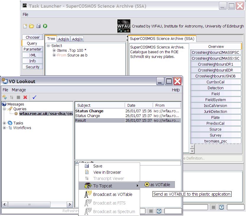
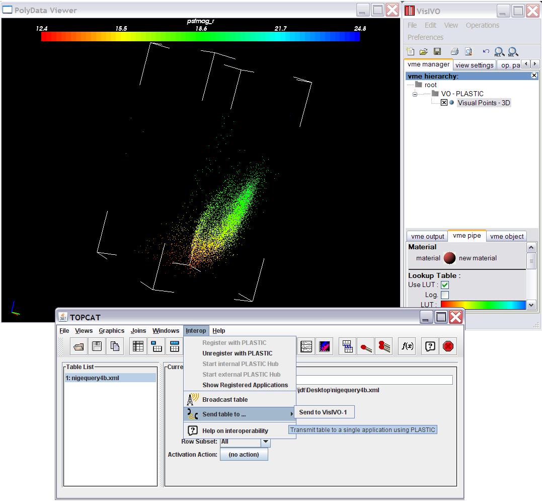
The following example illustrates how VisIVO’s PLASTIC interaction works in practice, with several applications exploiting each other’s strengths to explore data taken from the paper by Digby et al. (Digby, 2003). The AstroGrid Workbench (Workbench, ) is first used to search for suitable data in the SuperCOSMOS Science Archive (SSA, ) and Sloan Digital Sky Survey (SDSS, ). The astronomer begins his analysis by starting Topcat (Topcat, ), which connects to the Plastic Hub. The astronomer then uses PLASTIC to send the SuperCOSMOS data directly to Topcat (figure 3).
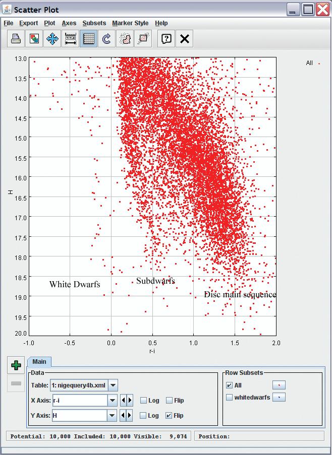
The SuperCOSMOS data does not contain the attributes that the astronomer needs, so he uses Topcat to add synthetic columns to calculate the colour indices of the sources and their reduced proper motions. A scatterplot of the r-i colour index against the reduced proper motion reveals that the sources fall into three populations: white dwarfs, sub dwarfs and main sequence stars (figure 4).
To fully understand this dataset the astronomer starts VisIVO, since it specializes in plotting multidimensional data. VisIVO connects with the Plastic Hub, and shortly afterwards the Workbench and Topcat’s menus update to reflect the fact that VisIVO is running and able to receive VOTables. The astronomer sends the augmented data from Topcat to VisIVO and uses VisIVO to create a 4D plot of r-i colour index, g-r colour index, reduced proper motion, and magnitude (using the latter to choose the colour of the points from a lookup table) (figure 5).
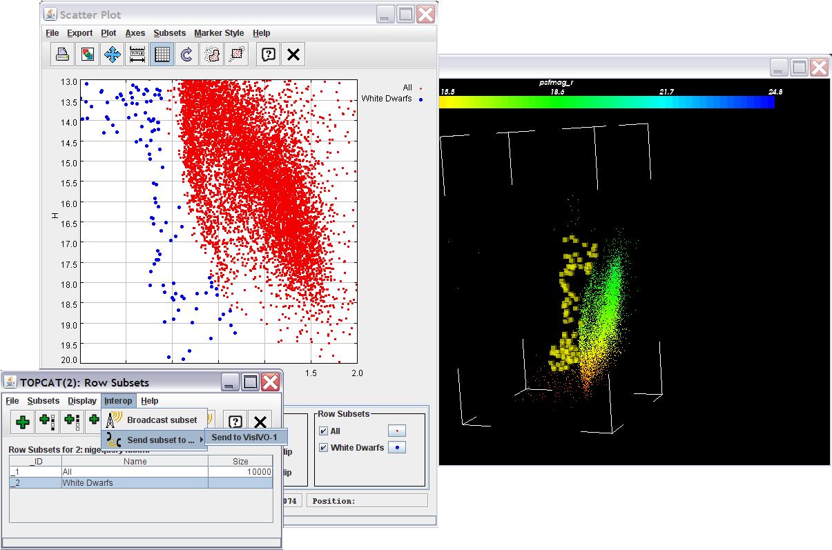
The white dwarf population can then be selected in Topcat and is automatically highlighted in VisIVO through PLASTIC for further exploration (figure 6). Finally, interesting objects can selected using VisIVO’s picker tool and sent via PLASTIC to Aladin for overlaying over an image so that the astronomer can see their spatial distribution. This workflow is, of course, greatly simplified. In reality the data would be transferred back and forth between VisIVO and other applications, with interesting clusters extracted and spurious data removed. It could be even be sent to statistical applications such as AstroWeka (AstroWeka, ) and Eirik (Eirik, ) to aid the astronomer in identifying clusters and trends.
While some of the above workflow could be accomplished by saving the dataset from one application and loading it in the next, PLASTIC makes the operation seamless.
4 Scientific cases
In this section, as an example of the practical usage of VisIVO, we will show how the tool can help the researcher in the analysis of two different problems: the classification of galaxies between star forming and quiescent objects and the detection of shock waves in galaxy clusters
4.1 Galaxies Classification
One of the most widely used methods relies on the intrinsic-colour versus absolute magnitude diagram: in this representations, redder objects, assumed to be quiescent, occupy a well defined locus, also known as red sequence. On the other hand, having spectroscopic information at hand, the equivalent width of the [OII] emission line is a well known tracer of on-going star formation activity, while the depth of the break at 4000 is an indicator of stellar age (the higher the break, the older the stellar population is). The question we ask ourselves is whether using one or the other of these indicators, we select the same population of galaxies, and also whether these indicators show some evolution with redshift. Starting from the VVDS epoch1 survey (Le Fèvre, 2005), we have extracted a subsample of galaxies with secure redshift, for which the equivalent width of the [OII] emission line (simply named [OII] from here on), and the depth of the 4000 break (from here on D4000) has been measured with good confidence (see Franzetti 2007 for details). Our global initial sample consists of 4640 galaxies, and for each object we have a measure of: V absolute magnitude, intrinsic U-V colour, redshift, [OII] and D4000. As a first step, we import the ASCII file where such information is stored into VisIVO, and do a first rough visualization of D4000 vs. [OII] vs. z. Such plot shows that there are 25 objects for which an anomalously large [OII] and/or D4000 has been measured. As we are currently interested in the global properties of the sample, and not in the outliers, we use the SubSample function to select the bulk of our data, eliminating such outliers. In figure 7a, the 3D representation of the D4000 vs. [OII] vs. z for the remaining objects is shown. The colour scale indicates the absolute magnitude associated to each object.
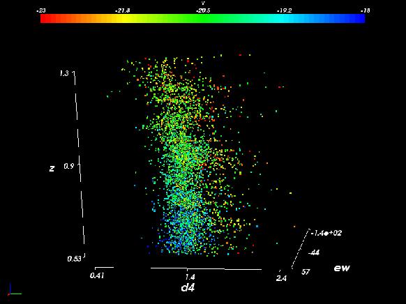
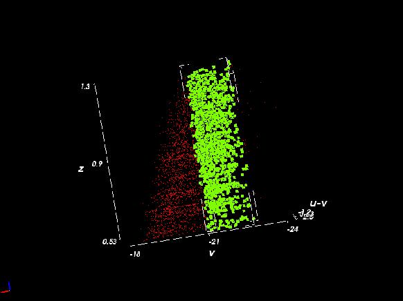
Two effects are immediately visible from figure 7a: the
first one is the to be expected selection effect on galaxy luminosity: the
further we go in redshift, the more luminous are the galaxies we have in
our sample (we have lesser and lesser blue points as redshift
increases). The second effect we see is a tendency
for D4000 to decrease with increasing redshift. Before further
inspecting this decrease, which can be scientifically very promising,
we get rid of the luminosity selection effect, by extracting from our global sample a volume limited
sub-sample, i.e. we include only objects having an absolute magnitude
visible throughout the whole redshift range. This is easily done
by displaying the absolute magnitude and redshift, and cut the sample
at an absolute magnitude using the SubSample
function (see figure 7b).
We save such selection in an ASCII file, for further use.
Now that we have a subsample clean from selection effects, we can go
back to our original problem, and first of all we want to see whether
the effect of D4000 decreasing as redshift increases is still noticeable.
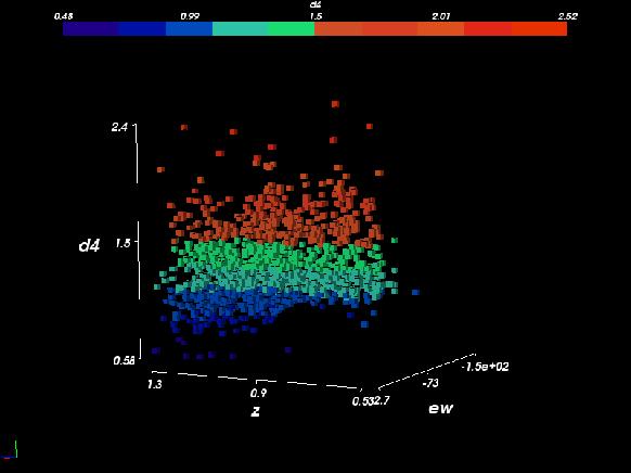
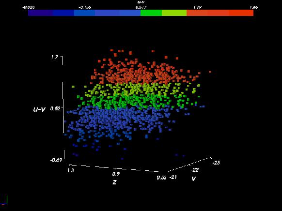
In fig. 8a, we show the D4000 vs. [OII] vs. z
datacube, where for clarity we use 4 different colours for different
D4000 ranges: at higher redshifts, not only
D4000 assumes smaller values, but rotating the cube we see that
[OII] has a tendency to be higher (on average) with increasing
redshift.
These two effects point towards a higher star forming rate at higher
redshift, and especially for . If we use the second
star-formation indicator, i.e. the colour magnitude diagram vs. redshift
(see fig. 8 b), we see again that at higher redshift, blue
galaxies are more abundant than red galaxies.
As a last point, we want to see whether galaxies which would be defined as
quiescent in a colour magnitude diagram are also spectroscopically
quiescent
(i.e. galaxies belonging to the red sequence should not show emission
lines), and vice-versa, if galaxies which show an old stellar
population
are indeed red in intrinsic colour.
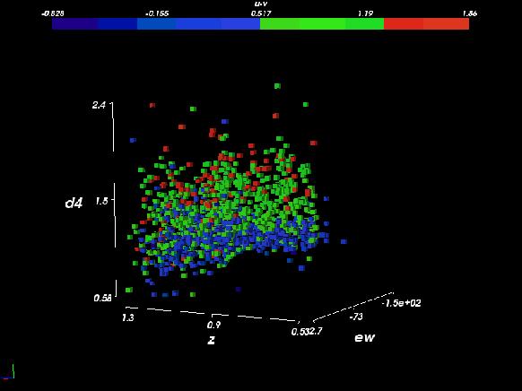
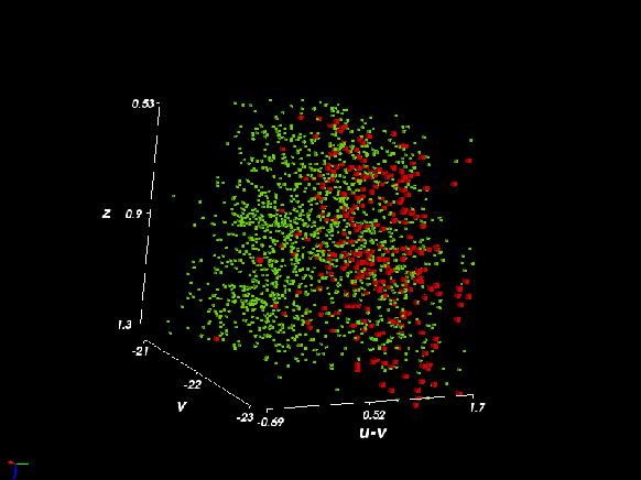
Displaying again the D4000 vs. [OII] vs. redshift data cube
(fig. 9a), we now
use colour to indicate the galaxy intrinsic U-V: as expected, red
galaxies show, on average, a higher stellar age indicator. Still,
there are some red galaxies showing a low value for D4000, as well as
blue galaxies with an old stellar population (high D4000), and
especially the intermediate class of colours (the green dots) span the
whole plane. This high degree of mixing does not seem to depend on
redshift. Also in the colour magnitude diagram
(fig. 9b), this is clearly visible: we have now
highlighted in red the galaxies which show a D4000 (old stellar
age) AND a low value of [OII] (no sign of star formation): these
galaxies have a tendency to have redder colours, but are not necessarily
the reddest ones, and not all the red
galaxies fall in this category
To summarize, using VisIVO exclusively, and without any programming
knowledge whatsoever, we have been able to inspect our sample and
1) see the volume selection and extract a bias free subsample,
2) find an interesting evolution of galaxy stellar age with redshift,
which deserves further statistical inspection (Vergani, 2007) for
a more exhaustive discussion of this topic),
3) show that selecting red galaxies on the basis of spectroscopic
features vs. photometric colours does not give the same sample. The
degree of contamination in the different cases is thoroughly
discussed in (Franzetti, 2007).
4.2 Detecting Shocks in Galaxy Clusters
Cosmic shock waves are believed to be among the most efficient accelerators of particles
in the universe. The final spectrum of
the accelerated particles is influenced by the complex interplay between the growth of
cosmic structures, the geometry of the shock waves and the number of shocks that a particle
may experience during its life.
A consistent and complete description of the dynamics of cosmological shock waves
is far from being achieved. However, numerical simulations provide a valuable
contribution to the comprehension of this process.
We have performed a large number of simulations using
the Enzo code, which is an adaptive mesh refinement cosmological code
(http://cosmos.ucsd.edu/enzo), developed by Bryan et al.
(Bryan, 1995). The Enzo code couples
an N-body particle-mesh solver with an PPM Eulerian adaptive method for ideal
gas-dynamics by Colella & Woodward 1984.
For all the runs, we adopted the standard ”Concordance” model, with
density parameters , , , , Hubble parameter and initial spectrum
normalization .
In order to have a large cluster statistics and a wide cosmological volume,
we simulated several datacubes, finally assembling an overall
volume of per side
Shocks identification has been performed using a novel method which studies the structure of the baryonic velocity field and evaluates Mach numbers through velocity jumps, developed by Vazza et al. (Vazza, 2007). Cells which present velocity jumps that can produce a shock wave (Landau, 1959) are tagged as shocked cells and their Mach number is estimated as:
| (3) |
where is the fluid velocity jump across the shock, in the reference
frame of the shock itself, .
This technique, coupled with the unprecedented good resolution
of our data in the outermost regions of virialized structures (where shocks very often occur),
allows us to study dynamical regimes never seen before. The use of a visualization code
such as VisIVO is of great importance because it allows us to detect
and follow the behaviours of shock patterns which are characterized by very complex
volume–filling properties, which had always been erased by most standard reduction analyses and
can be of primary importance to correctly describe the observational impact of these
mechanisms.
Data from the simulations are saved in raw binary and HDF5 formats,
which generates a huge data collection.
In the following, for simplicity, we will focus on the results of one of the simulations,
characterized by mesh cells and the same number of N-Body particles.
The computational box is 40 Mpc and the presented results are at redshift .
However, all the conclusions can be extended to all the outputs of our data
collection. VisIVO is used to explore in an intuitive and effective way
the data and to focus on the interesting and, sometimes, unexpected aspects.
Data have been combined
using the Merge Tables function. The Math Op. tools have been used to derive
new datasets, like logarithmic quantities or velocity magnitude.
Cosmological simulations produce extremely complex
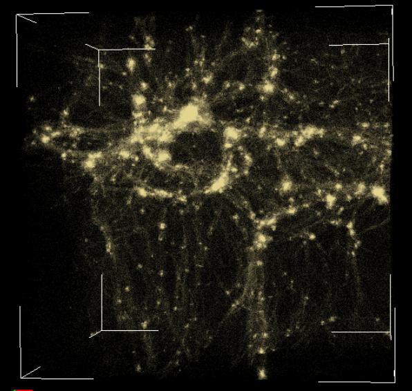
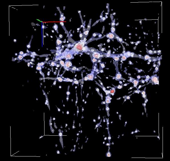
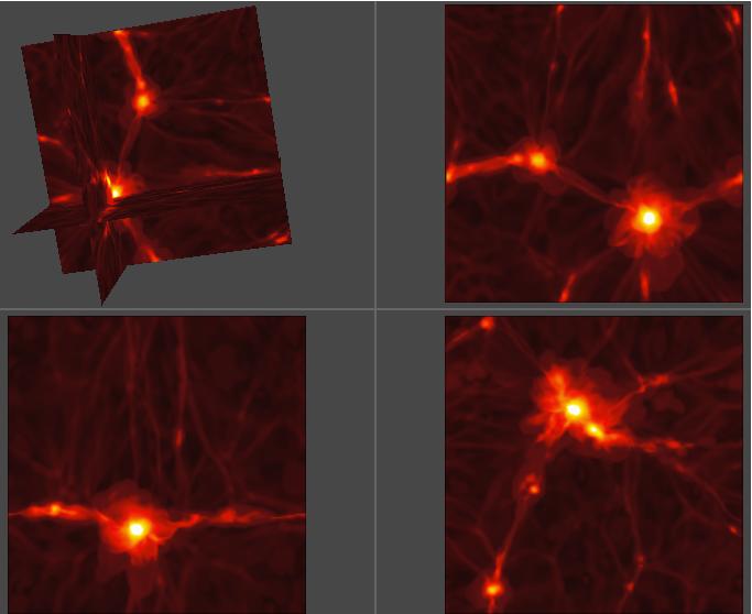
structures, characterized by clumps, filaments, sheets, large voids etc. In figure 10,
the distribution of particles representing the dark matter is shown in the top
panel. The bottom panel presents a comparison between the dark matter and the gas mass
distributions, these two quantities being represented by isosurfaces. Red and light blue isocontours show
the gas distribution at different mass density values. For comparison, dark matter isosurfaces
(in white colour) are superimposed. Dark matter mass density is calculated by smoothing
the particle masses on the computational grid using the VisIVO point distribute function.
Gas and Dark matter mass distributions are similar, since they are both driven
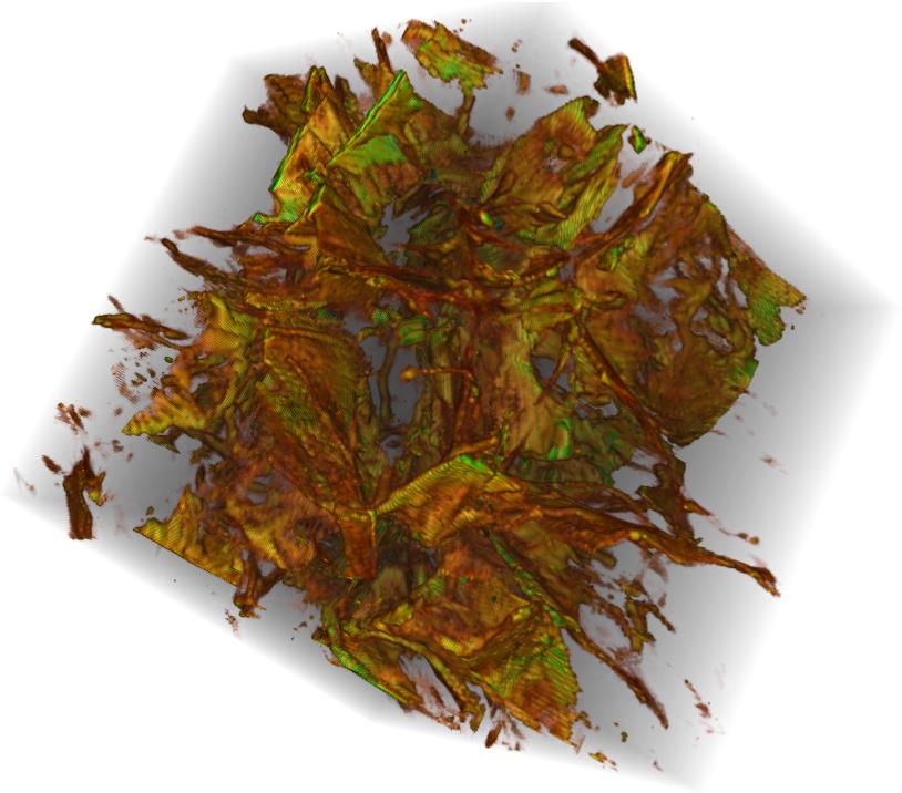
by a common gravitational potential. The temperature distribution, shown in the top panel figure
11 using a volume rendering technique, follows the overall mass distribution.
However, a shock wave which forms during the gravitational collapse events expands rapidly,
raising the gas temperature to -K on volumes up to Mpcs.
In order to have a quantity directly comparable to observations, we have
calculated the gas X-ray emission due to thermal bremsstrahlung
directly using the VisIVO Math tool. The X-ray
distribution is shown using the VisIVO slider utility in the bottom panel of
figure 11. As expected the emission is strongly associated with the
clusters, since it depends principally on the mass concentration.
Once general features of the data have been analyzed, we switch to the identification and characterization of shocks. Shock fronts and the corresponding Mach numbers are identified by our velocity-jumps based procedure. The shocks-density distribution is presented in figure 12.
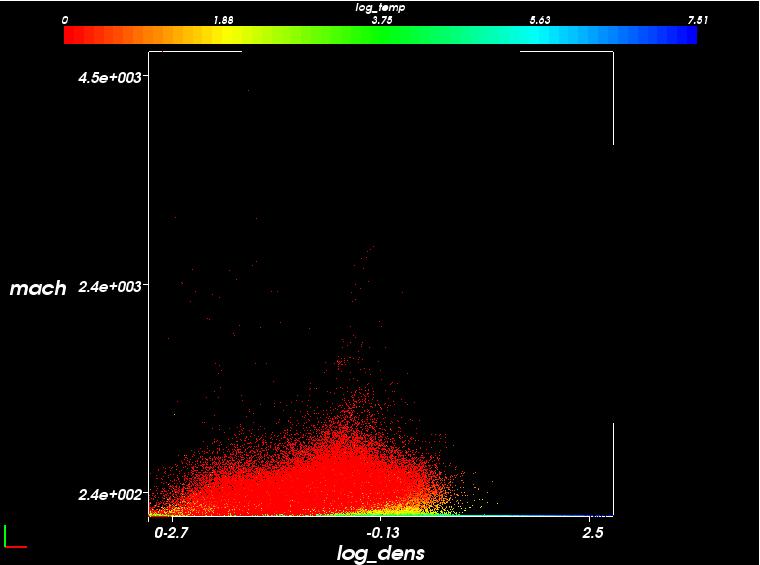
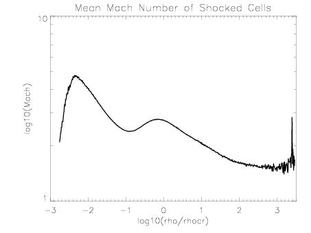
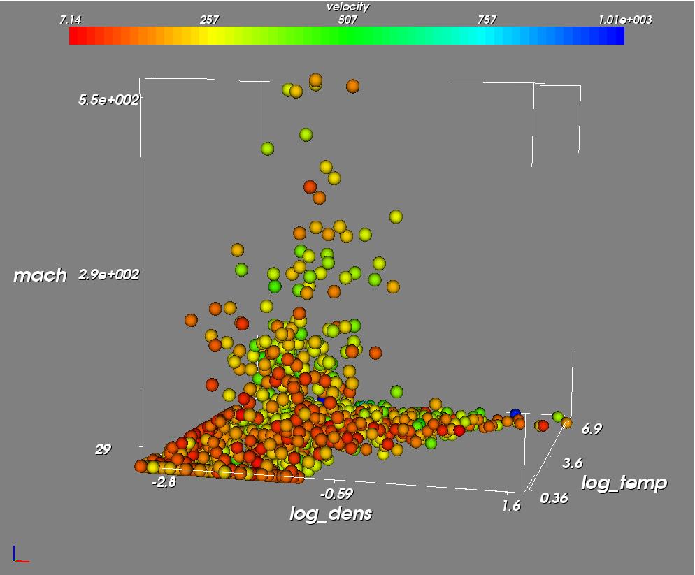
In the top panel, points are coloured according to their temperature.
Most of the high Mach (Mach number ) shocks are in low temperature regions, therefore
far outside the galaxy cluster virial radius.
The distribution present two peaks corresponding to different values of
density. The right peak (larger density value) is observed in any kind of simulation
and it corresponds to shocks forming in the outer outskirts of clusters
and along filaments, where the matter accretion is still strong.
The left peak corresponds to rare voids, which represent the low density tail of the
probability density function in a CDM universe. It
has never been detected in any previous numerical simulations. The double peaked feature
of the distribution is confirmed when all the dataset available in our collection, are taken into
account, as shown in bottom panel of figure 12.
This result is determined both by the improved accuracy of our
shock reconstruction algorithm and by the simulations code. In fact
some of the previous studies are related to SPH based simulation, which cannot
treat in a proper way the hydrodynamics of underdense regions, that are poorly
sampled by the particle based approach.
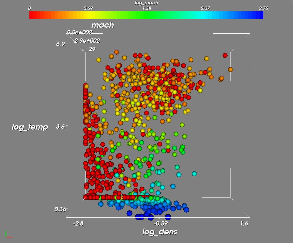
Figure 13 shows a 4D phase space distribution of a subsample
of points extracted from the whole simulation. The VisIVO Randomizer function
allows the user to select a small number of points in order to proceed
faster in the analysis, without requiring huge computational
resources. The figure shows the density-temperature-mach number distribution
of sampled points, which are further coloured by the mach number itself (top panel)
and the velocity (bottom panel). The top panel shows that high mach points (blue
spheres) are concentrated at low temperature. High density regions also have
high temperatures. However, low density regions, have temperatures in a wide
range, from to K. This is due to the fast shock propagation
outside collapsing structures (see also figures 10 and 11).
The bottom panel emphasizes the density-mach number relation. It is still present,
even if less clear, due to lower statistics, the low density
Mach number peak. The L-shaped phase space distribution
(high mach-low temperatures, low mach-high temperatures) is also evident. The velocity
seems not to present a specific trend with respect to the other quantities.
All these features
are present also using the complete dataset and
in any other random extraction, proving that there are not
spurious effects connected to statistical biases.
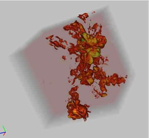
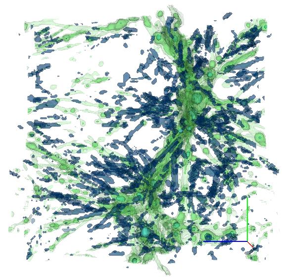
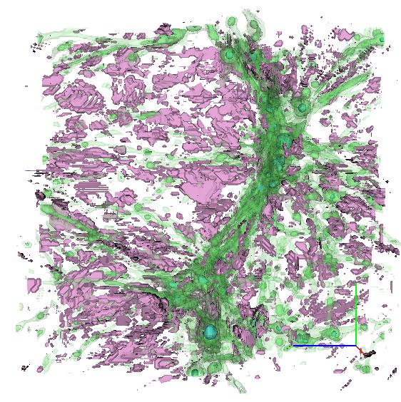
In figure 14, we show the geometric distribution of the shocks,
visualized as 3D surfaces with Mach and selected according to the mass density
values. The top panel shows the shocks on the high density
peak of the figure 12 distribution. The bottom panel shows the shocks
in low density regions.
The presence of such vast surfaces of high mach shock in
underdense regions suggests that these regions must be carefully taken into account, in order to properly
evaluate the net amount of energy which ends up in particles re-acceleration (Brunetti, 2003).
A further analysis of the data is ongoing. Quantitative data analysis tools are
at this point necessary to estimate the results that have been revealed and
emphasized using VisIVO. The method proved to be extremely
effective in getting an immediate and effective approach to a complex and huge
dataset, selecting and extracting interesting features, which would otherwise be hardly
detectable.
5 Summary
In the previous sections we have shown how an advanced visualization tool like VisIVO can be used for helping the researcher in analyzing complex data. Visualization cannot provide quantitative results, but it allows the user to have an immediate and intuitive approach to the data. The various 3D rendering techniques supported by VisIVO, together with the possibility of visualizing complementary quantities with colours, glyphs and vectors, allows the user to discriminate between data features at a glance, pointing out special characteristics and focusing on interesting regions. The software also implements a limited but effective set of statistical tools, that can be used to make quick estimates of the properties of a distribution. Mathematics functions let the user derive new fields starting from the original ones. VisIVO is being developed to follow the IVOA recommendations and standards, so that it is interoperable with the Virtual Observatory framework. Furthermore, it supports the PLASTIC protocol to allow the user to use the software together with other tools, such as Aladin or Topcat, which have complementary data analysis capacities to those of VisIVO. In this way the researcher can have a complete and customized cooperating set of tools that makes his/her research activity more and more efficient and focused on scientific issues.
New features of VisIVO will focus on exploiting new hardware architectures that are rapidly appearing in many desktop machines, such as 64 bit and multicore systems, subject to making effective use of such capabilities in the tool. The opportunity to use VisIVO in data centres and on dedicated visualization servers will drive the new releases of the code. We will also investigate the possibility of interacting with remote data services that support the SNAP protocol, which is an emerging protocol for retrieving data from numerical simulations. Finally, VisIVO will be developed to integrate with the VO’s Theoretical Data Archive framework. VisIVO will display a subset of the whole data file, which will generally be very large, and will allow the user to select a spherical or rectangular region and retrieve, through a remote service, the extracted sub-sample.
References
- Bonnarel (2000) Bonnarel F. et al., 2000, A&AS, 143, 33
- Brunetti (2003) Brunetti G. Matter and Energy in Clusters of Galaxies, ASP Conference Proceedings, 2003, Stuart Bowyer and Chorng-Yuan Hwang. San Francisco: Astronomical Society of the Pacific, 2003, page 349
- Bryan (1995) Bryan G.L., Norman M.L., Stone J.M., Cen R.Y., Ostriker J.P., 1995, Comput. Phys. Comm., 89, 149
- Colella (1985) Colella P., Woodward P., 1984, J. Comput. Phys., 54, 174
- Coles (2002) Coles P. and Lucchin F.Cosmology. The Origin and Evolution of Cosmic Structure. 2002, John Wiley and Sons
- Digby (2003) Digby A.P. et al., 2003, The subdwarf luminosity function, MNRAS, 344, 583
- Franzetti (2007) Franzetti P., et al., 2007, A&AS, in press.
- Landau (1959) Landau L.D., Lifshits E.M., 1959, Fluid Dynamics. Pergamon Press Ltd., London
- Le Fèvre (2005) Le Fèvre O., et al., 2005, A&AS, 439,845.
- Ochsenbein (2000) Ochsenbein F., Bauer P., Marcout J., 2000, A&AS 143, 221
- Peebles (1974) Peebles P. J. E., Hauser M. G., 1974, ApJS, 28, 19
- Platzoder (1995) Platzoder M, and Buchert T. Applications of Minkowski-functionals to the Statistical Analysis of Dark Matter Models. 1995, A. Weiss, G. Raelt, W. Hillebrandt, and F. von Feilitzsch, Proc. of 1st SFB workshop on Astro-particle physics, Ringberg, Tegernsee , pages 251
- Schroeder (2004) Schroeder W., Martin K., Lorensen B., The Visualization Toolkit An Object-Oriented Approach To 3D Graphics 3rd Edition, 2004, Kitware Inc., ISBN-1-930934-12-2
- Springel (2000) Springel,V. 2000, MNRAS 1105, 364
- Taylor (2006) Taylor J.D. et al., 2006, PLASTIC - a protocol for desktop application interoperability, IVOA Note http://ivoa.net/Documents/latest/PlasticDesktopInterop.html
- Vazza (2007) Vazza F., Brunetti G., Gheller C. 2007, in preparation
- Vergani (2007) Vergani,D., et al., 2007, in preparation.
- Viceconti (2004) Viceconti M. et al.. The Multimod Application Framework IEEE Proceedings of IV’ 2004, 15
- Winstanley (2006) Winstanley, N. et al, 2006, Astro Runtime - Client-Side Middleware for the VO, ADASS 2006 Proceedings, in press
- (20) http://www2.astrogrid.org/desktop
- (21) http://surveys.roe.ac.uk/ssa/
- (22) http://www.sdss.org/
- (23) http://astroweka.sourceforge.net
- (24) http://aladin.u-strasbg.fr/java/nph-aladin.pl?frame=plugins
- (25) http://wiki.eurovotech.org/twiki/bin/view/VOTech/EirikDemo
- (26) http://cm.bell-labs.com/who/tkh/mirage/index.html
- (27) http://www.starlink.ac.uk/topcat/
- (28) http://eurovotech.org
- (29) http://davis.wpi.edu/xmdv/
- (30) http://esavo02.esac.esa.int:8080/vospec/
- (31) http://www.eso.org/sampo/reflex/