We present a new prescription for the resummation of the divergent series of perturbative corrections, due to soft gluon emission, to hard processes near threshold in perturbative QCD (threshold resummation). This prescription is based on Borel resummation, and contrary to the commonly used minimal prescription, it does not introduce a dependence of resummed physical observables on the kinematically unaccessible $x\to 0$ region of parton distributions. We compare results for resummed deep-inelastic scattering obtained using the Borel prescription and the minimal prescription and exploit the comparison to discuss the ambiguities related to the resummation procedure.

July 2007

The resummation of logarithmically enhanced contributions to hard processes near threshold [1, 2], such as deep-inelastic scattering and Drell-Yan production at large values of the Bjorken $x$ variable (or its analogue in the case of Drell-Yan), is characterized by the fact that the effective scale of the process is a soft scale related to the emission process. This means that for a process with hard scale $Q^{2}$ the resummation of large logs of $1-x$ effectively replaces the perturbative coupling $\alpha_{s}(Q^{2})$ with $\alpha_{s}(Q^{2}(1-x))$. In the space of the variable $N$ which is conjugate to $x$ upon Mellin transformation, where the resummation is more naturally performed, the effective coupling is $\alpha_{s}(Q^{2}/N)$ and the soft limit $x\to 1$ corresponds to $N\to\infty$. This result, which has been understood long ago [3] on the basis of an analysis of evolution equations in the soft limit, and more recently in terms of effective theories [4], is a simple consequence of the fact [5] that in the soft limit cross sections only depend on $x$ through the soft scale $Q^{2}(1-x)$, so this dependence can be renormalization–group improved using standard techniques.

As the scale decreases, the strong coupling increases and eventually it blows up at the Landau pole, so when

$$x=x_{L}\equiv 1-\frac{\Lambda^{2}}{Q^{2}}$$ (1)

resummed results diverge, and physical observables can be determined only by specifying a prescription to treat this divergence. A simple option, already discussed in ref. [3], is to perform the resummation in $x$ space and cut off the phase space integration so that the dangerous $x\geq x_{L}$ region is excluded. The option which is more commonly used, however, is to perform the resummation in $N$ space, and reconstruct the result in $x$ space by Mellin inversion. In this case, if the Mellin inversion is performed order by order in perturbation theory, the series of resummed $x$-space contributions diverges, and the problem is turned into that of summing a divergent series [6].

A commonly used way of treating this divergent series is the minimal prescription (MP) [6], which, as we shall discuss in more detail, is based on the observation that the Mellin inversion integral of the resummed $N$ space result exists if performed along a suitable contour. Furthermore, the divergent series obtained from the order-by-order Mellin inversion is an asymptotic expansion of this integral. The minimal prescription, however, has the shortcoming that upon convolution the partonic cross section does not vanish in the unphysical $x>1$ region, which implies that physical observables pick up a power-suppressed contribution from the unaccessible $x\to 0$ region of parton distributions.

In ref. [7] some of us suggested instead that the divergent series could be summed using the Borel method, and showed how this can be done at the leading logarithmic level for the logarithmic derivative of the resummed partonic cross section. Here we show how to perform this Borel resummation at any desired logarithmic order for any physical observable (such as, say, the DIS or Drell-Yan cross section at the hadronic level): namely, we give here a general Borel resummation prescription (BP). The availability of several resummation prescriptions is per se useful as a way of estimating the uncertainty of the resummation procedure. More interestingly, we will show that the Borel prescription solves the aforementioned problem of the minimal prescription. Indeed, the BP leads to a resummed partonic cross section which has the form of an $x$–space plus distribution, such as found at finite perturbative order, and thus gives physical observables by a convolution with parton distributions in the standard way. This is achieved through the inclusion of a higher twist term in the resummed result.

We will first summarize the properties of the resummed result and in particular the divergence of the resummed perturbative expansion. We will then describe the Borel resummation of the resummed partonic cross section, and specifically discuss its dependence on the choice of higher twist terms included in it. Finally we will compare the Borel prescription to the minimal prescription, and in particular compare results for physical observables obtained using either method.

In order to understand the origin of the divergence of resummed results, let us consider first as an example the computation of the resummed leading log expression of

$$\gamma(\alpha_{s}(Q^{2}),N)\equiv\frac{\partial\ln\hat{\sigma}(\frac{Q^{2}}{\mu^{2}},\alpha_{s}(\mu^{2}),N)}{\partial\ln Q^{2}},$$ (2)

where $\hat{\sigma}\left(\frac{Q^{2}}{\mu^{2}},\alpha_{s}(\mu^{2}),N\right)$ is the Mellin transform

$$\hat{\sigma}\left(\frac{Q^{2}}{\mu^{2}},\alpha_{s}(\mu^{2}),N\right)=\int_{0}^{1}\!dx\,x^{N-1}\bar{\sigma}\left(\frac{Q^{2}}{\mu^{2}},\alpha_{s}(\mu^{2}),x\right)$$ (3)

of an observable $\bar{\sigma}\left(\frac{Q^{2}}{\mu^{2}},\alpha_{s}(\mu^{2}),x\right)$ such as the Drell-Yan cross section or a deep-inelastic structure function, computed at the parton level. In the soft limit, $\gamma(\alpha_{s}(Q^{2}),N)$ is computed up to terms which do not grow as $N\to\infty$, and at the leading logarithmic level, it is a function of $\alpha_{s}(Q^{2})\ln\frac{1}{N}$ only. Explicitly,

$$\gamma_{LL}(\alpha_{s}(Q^{2}),N)=g_{1}\int_{1}^{N^{a}}\frac{dn}{n}\,\alpha_{s}(Q^{2}/n)=-\frac{g_{1}}{\beta_{0}}\ln\left[1+\bar{\alpha}\ln\frac{1}{N}\right].$$ (4)

where $g_{1}$ is a constant, $a=1$ for deep–inelastic scattering and $a=2$ for Drell-Yan, we have used the explicit leading log form of $\alpha_{s}(Q^{2})$,

$$\alpha_{s}(Q^{2})=\frac{\alpha_{s}(\mu^{2})}{1+\beta_{0}\alpha_{s}(\mu^{2})\ln\frac{Q^{2}}{\mu^{2}}};\qquad\beta_{0}=\frac{33-2n_{f}}{12\pi},$$ (5)

and we have defined

$$\quad\bar{\alpha}\equiv a\beta_{0}\alpha_{s}(Q^{2}).$$ (6)

Clearly, $\gamma_{LL}(\alpha_{s}(Q^{2}),N)$ has a branch cut on the positive real axis of the complex $N$ plane, starting at the Landau pole of $\alpha_{s}$ eq. (5),

$$N_{L}=e^{\frac{1}{\bar{\alpha}}}.$$ (7)

But if $\gamma_{LL}(\alpha_{s}(Q^{2}),N)$ were the Mellin transform of some function $P_{LL}(\alpha_{s}(Q^{2}),x)$, it would be regular above some abscissa of convergence $N_{c}$, i.e. for all $\hbox{Re}(N)>N_{c}$. Hence, $\gamma_{LL}(\alpha_{s}(Q^{2}),N)$ is not the Mellin transform of anything. However, to any finite fixed perturbative order $M$ the inverse Mellin transform of $\gamma(\alpha_{s}(Q^{2}),N)$ is given by

$$P^{(M)}(\alpha_{s}(Q^{2}),x)=-\frac{g_{1}}{\beta_{0}}\sum_{k=1}^{M}\frac{(-1)^{k+1}}{k}\bar{\alpha}^{k}\,\frac{1}{2\pi i}\int_{\bar{N}-i\infty}^{\bar{N}+i\infty}dN\,x^{-N}\ln^{k}\frac{1}{N};\qquad\bar{N}>0,$$ (8)

where all Mellin inversion integrals can be computed exactly [see the appendix, eq. (69)]. It is easy to see that the limit of $P^{(M)}(\alpha_{s}(Q^{2}),x)$ as $M\to\infty$ diverges. Indeed, if the limit existed, then one could interchange the sum over $k$ and the integral over $N$, but the sum over $k$ is then the Taylor expansion of $\gamma_{LL}(\alpha_{s}(Q^{2}),N)$ eq. (2), which has finite radius of convergence $|N|<N_{L}$, whereas the $N$ integral extends to infinity.

In ref. [7] we have computed the divergent series eq. (8) explicitly and summed it à la Borel. The approach of that reference however exploits the explicit form of $\gamma_{LL}(\alpha_{s}(Q^{2}),N)$ eq. (4), and in particular the fact that the integrand in eq. (4) has a simple pole. We now present a generalization of that method which reduces to it in the case of $\gamma_{LL}(\alpha_{s}(Q^{2}),N)$, but can be applied to any resummed quantity.

We start with a Mellin-space resummed quantity $\Sigma$, function of $\alpha_{s}(Q^{2})$, $\ln\frac{1}{N}$ and possibly other kinematical variables such as the rapidity, which we will not indicate explicitly. This resummed quantity is related to the partonic cross section $\hat{\sigma}\left(\frac{Q^{2}}{\mu^{2}},\alpha_{s}(\mu^{2}),N\right)$ eq. (3), or a quantity derived from it such as $\gamma$ eq. (2). Now, in the soft limit $\hat{\sigma}$ eq. (3) can be expanded as [6]

$$\hat{\sigma}\left(\frac{Q^{2}}{\mu^{2}},\alpha_{s}(\mu^{2}),N\right)=\hat{\sigma}_{0}\exp\left[\ln\frac{1}{N}g_{1}\left(\bar{\alpha}\ln\frac{1}{N}\right)+g_{2}\left(\bar{\alpha}\ln\frac{1}{N}\right)+\alpha_{s}(Q^{2})g_{3}\left(\bar{\alpha}\ln\frac{1}{N}\right)+\dots\right],$$ (9)

where $\hat{\sigma}_{0}$ is the Born level result. It is thus convenient to expand the generic resummed quantity $\Sigma$ as

$$\Sigma\left(\alpha_{s}(Q^{2}),L\right)=\lim_{M\to\infty}\sum_{k=1}^{M}h_{k}(\alpha_{s}(Q^{2}))L^{k}$$ (10)

where we have defined

$$L\equiv\bar{\alpha}\ln\frac{1}{N}=a\beta_{0}\alpha_{s}(Q^{2})\ln\frac{1}{N},$$ (11)

with $\alpha_{s}(Q^{2})$ not necessarily given by its leading order expression. In the case of the computation of the partonic cross section, $\Sigma\left(\alpha_{s}(Q^{2}),L\right)$ is explicitly given by

$$\hat{\sigma}\left(\frac{Q^{2}}{\mu^{2}},\alpha_{s}(\mu^{2}),N\right)=\hat{\sigma}_{0}\left[1+\Sigma\left(\alpha_{s}(Q^{2}),L\right)\right].$$ (12)

For a generic resummed observable the series eq. (10) has finite radius of convergence $|L|<1$ dictated by the location of the Landau pole. Hence the term-by-term inverse Mellin of the series eq. (10) is divergent. The divergent series can be determined explicitly [7] [see eq. (69) of the appendix] to compute the inverse Mellin transform of $\Sigma\left(\alpha_{s}(Q^{2}),L\right)$ eq. (10), but with $M$ kept finite,

$$\bar{\Sigma}^{M}\left(\alpha_{s}(Q^{2}),x\right)\equiv\int_{\bar{N}-i\infty}^{\bar{N}+i\infty}\!\frac{dN}{2\pi i}\,x^{-N}\Sigma\left(\alpha_{s}(Q^{2}),L\right),\qquad\hbox{$M$ finite }.$$ (13)

We get

$$\bar{\Sigma}^{M}\left(\alpha_{s}(Q^{2}),x\right)=\left[\frac{R^{M}(x)}{1-x}\right]_{+}+O\left[(1-x)^{0}\right],$$ (14)

$$\>R^{M}(x)=\sum_{n=0}^{M}\Delta^{(n)}\left(1\right)\sum_{k=n}^{M}\left(\begin{array}[]{c}k\\ n\end{array}\right)c_{k}\bar{\alpha}^{k+1}\ell^{k-n}+O\left[(1-x)^{0}\right],$$ (17)

where we have defined

$$c_{k}\equiv(k+1)h_{k+1};\quad\ell\equiv\ln(1-x),$$ (18)

$\Delta^{(n)}(z)$ is the $n$-th derivative of

$$\Delta(z)\equiv\frac{1}{\Gamma(z)},$$ (19)

$O\left[(1-x)^{0}\right]$ denotes terms which are nonsingular in the limit $x\to 1$, and for brevity we have omitted the explicit dependence of the coefficients $h_{k}$ and of $R^{M}$ on $\alpha_{s}(Q^{2})$. The divergent series which we wish to sum is then

$$R(x)=\lim_{M\to\infty}R^{M}(x).$$ (20)

The divergence of $R(x)$ can be removed by performing a Borel transform with respect to $\bar{\alpha}$, which gives

$$\hat{R}(w,x)=\sum_{n=0}^{\infty}\frac{\Delta^{(n)}\left(1\right)}{n!}\sum_{k=n}^{\infty}\frac{c_{k}}{\left(k-n\right)!}w^{k}\ell^{k-n}.$$ (21)

The inner series has an infinite radius of convergence because its coefficients are factorially smaller than those of the series eq. (10). Because $\Delta(z)$ eq. (19) is an entire function of $z$, it is easy to show that this implies that the outer series is also convergent. Indeed, because the series $\sum_{k}c_{k}z^{k}$ is convergent with the same radius as the series eq. (10), as $k\to\infty$ the coefficients $c_{k}$ are bounded by some constant $K>0$, $|c_{k}|<K$. But this implies

$$|\hat{R}(w,x)|\leq K\sum_{n=0}^{\infty}\frac{|\Delta^{(n)}\left(1\right)|}{n!}\sum_{k=n}^{\infty}\frac{1}{\left(k-n\right)!}|w^{k}\ell^{k-n}|=Ke^{|w\ell|}\sum_{n=0}^{\infty}\frac{|\Delta^{(n)}\left(1\right)|}{n!}|w|^{n}$$ (22)

which converges because of the absolute convergence of the power series for $\Delta(z)$ eq. (19).

The original series can be recovered by inverting the Borel transform,

$$R(x)=\int_{0}^{\infty}\!dw\,e^{-\frac{w}{\bar{\alpha}}}\hat{R}(w,x),$$ (23)

but the integral over $w$ in eq. (23) diverges at infinity: indeed, if we integrate the series term by term we recover the original divergent series eq. (17). We can cut off the singularity by extending the integral only up to some upper bound $C$. Because the series eq. (21) converges uniformly in the interval $0\leq w\leq C$, we can integrate term by term, with the result

$$R_{B}\left(x,C\right) = \int_{0}^{C}\!dw\,e^{-\frac{w}{\bar{\alpha}}}\hat{R}(w,x)$$ (24)

$$= \sum_{n=0}^{\infty}\Delta^{(n)}\left(1\right)\sum_{k=n}^{\infty}\left(\begin{array}[]{c}k\\ n\end{array}\right)c_{k}\frac{\gamma\left(k+1,\frac{C}{\bar{\alpha}}\right)}{k!}{\bar{\alpha}}^{k+1}\ell^{k-n},$$ (27)

where

$$\gamma(k+1,z)\equiv\int_{0}^{z}\!dw\,e^{-w}w^{k}=k!\left(1-e^{-z}\sum_{n=0}^{k}\frac{z^{n}}{n!}\right)$$ (28)

is the truncated gamma function. The series eq. (27) for $R_{B}\left(x,C\right)$ has infinite radius of convergence, like that for $\hat{R}(w,x)$ eq. (21).

The Borel resummation of $\bar{\Sigma}\left(\alpha_{s}(Q^{2}),x\right)$ is obtained substituting the expression for $R_{B}\left(x,C\right)$ eq. (27) in eq. (14). Equation (27) is not vey useful because it requires the evaluation of a double series. However, we will now show that the series can be summed through an integral representation which is not harder to evaluate numerically than the minimal prescription. Before doing this, let us discuss the properties of the Borel resummation.

First, it is easy to see that the divergent series we started from $R(x)$ eq. (17) is an asymptotic expansion of its Borel resummation $R_{B}\left(x,C\right)$ eq. (27). To this purpose, we note that $R(x)$ and $R_{B}\left(x,C\right)$ are related by

$$R_{B}\left(x,C\right)=R(x)-R_{ht}(x,C),$$ (29)

where, using eq. (28),

$$R_{ht}(x,C)=e^{-\frac{C}{\bar{\alpha}}}\sum_{n=0}^{\infty}\Delta^{(n)}\left(1\right)\sum_{k=n}^{\infty}\left(\begin{array}[]{c}k\\ n\end{array}\right)c_{k}\ell^{k-n}\sum_{m=0}^{k}\frac{1}{m!}\left(\frac{C}{\bar{\alpha}}\right)^{m}\bar{\alpha}^{k+1}.$$ (30)

Hence, $R_{ht}\sim e^{-\frac{1}{\bar{\alpha}}}$, so it vanishes faster than any power of $\alpha_{s}(Q^{2})$ as $\alpha_{s}(Q^{2})\to 0$. It follows that the difference between $R_{B}\left(x,C\right)$ and the sum of the first $N$ terms of $R\left(x\right)$ is of order $\alpha_{s}(Q^{2})^{N+1}$, which proves that $R\left(x\right)$ is an asymptotic expansion of $R_{B}\left(x,C\right)$.

Furthermore, note that using the expression for $\alpha_{s}(Q^{2})$

$$\alpha_{s}(Q^{2})=\frac{1}{\beta_{0}\ln\frac{Q^{2}}{\Lambda^{2}}}\left[1+O(\alpha_{s}(Q^{2}))\right]$$ (31)

we get

$$e^{-\frac{C}{\bar{\alpha}}}=\left(\frac{\Lambda^{2}}{Q^{2}}\right)^{C/a}\left[1+O(\alpha_{s}(Q^{2}))\right].$$ (32)

This shows that cutting off the Borel inversion integral eq. (23) at $w=C$ is equivalent to including a twist-$t$ contribution $R_{ht}(x,C)$, with

$$t=2+\frac{2C}{a}.$$ (33)

The divergence of the higher twist term then cancels that of the divergent series, leading to a finite result. The value of $C$ should be chosen in such a way that no new, spurious higher twist terms are induced in physical observables. The choice $C=a$ is minimal in that it corresponds to the inclusion of a twist-four term, i.e. a term of the first subleading twist.

Let us now turn the Borel resummed expression $R_{B}\left(x,C\right)$ eq. (27) into a more useful form. In order to perform the sum over $n$, we introduce the Fourier transform

$$\tilde{\Delta}_{\eta_{0}}\left(\zeta\right)\equiv\int_{-\infty}^{\infty}\frac{d\eta}{2\pi}e^{-i\zeta\eta}\Delta\left(1+\eta\right)\Theta(\eta+\eta_{0})$$ (34)

which satisfies

$$\int_{-\infty}^{\infty}d\zeta e^{i\eta\zeta}\tilde{\Delta}_{\eta_{0}}\left(\zeta\right)=\Delta(1+\eta)\Theta(\eta+\eta_{0}),$$ (35)

where $\Theta(\eta)$ is the Heaviside step function, and it is necessary to introduce a cutoff at $\eta_{0}$ because the Fourier transform of the function $\Delta(z)$ does not exist. Rewriting $R_{B}\left(x,C\right)$ eq. (24,21) with

$$\Delta^{(n)}(1)=\int_{-\infty}^{\infty}\!d\zeta\,\tilde{\Delta}_{\eta_{0}}\left(\zeta\right)\left(i\zeta\right)^{n}$$ (36)

we can perform the sum over $n$ explicitly:

$$R_{B}\left(x,C\right)=\int_{0}^{C}\!dw\,e^{-\frac{w}{\bar{\alpha}}}\int_{-\infty}^{\infty}\!d\zeta\,\tilde{\Delta}_{\eta_{0}}\left(\zeta\right)\sum_{k=0}^{\infty}\frac{c_{k}}{k!}\left[w\left(\ell+i\zeta\right)\right]^{k}.$$ (37)

where it is sufficient to choose $\eta_{0}>0$ to ensure that the result is independent of the choice of $\eta_{0}$.

Figure 1: The Hankel contour used in eq. (38).

Now, we observe that the sum over $k$ can be performed explicitly if the factor of $k!$ in the denominator is removed. We do this as follows. First, we write $1/k!=1/\Gamma(k+1)$ and we use the Hankel representation of the Gamma function

$$\frac{1}{\Gamma\left(z\right)}=-\int_{H}\frac{dt}{2\pi i}e^{-t}\left(-t\right)^{-z},$$ (38)

where $H$ is the Hankel contour shown in fig. 1. Furthermore, because the integrand in eq. (38) doesn’t have any other singularities in the complex plane besides the cut along the positive real axis, the integral along the Hankel contour $H$ is equal to the integral along the contour $H_{1}$ defined by

$$z_{H_{1}}=Re^{i\theta},$$ (39)

with $R\to\infty$ and $\epsilon\leq\theta\leq 2\pi-\epsilon$ with $\epsilon\to 0$. If we substitute in eq. (37) the expression eq. (38) with $z=k+1$ and the integral over $t$ performed along $H_{1}$ we can integrate term by term over $t$ the sum over $k$, because the contour $H_{1}$ is always within the radius of convergence of the series if $R$ eq. (39) is large enough. We get

$$R_{B}\left(x,C\right) = \int_{0}^{C}\!dw\,e^{-\frac{w}{\bar{\alpha}}}\int_{-\infty}^{\infty}d\zeta\tilde{\Delta}_{\eta_{0}}\left(\zeta\right)\int_{H_{1}}\frac{dt}{2\pi it}e^{-t}\sum_{k=0}^{\infty}c_{k}\left[-\frac{w}{t}\left(\ell+i\zeta\right)\right]^{k}$$ (40)

$$= \int_{0}^{C}\!dw\,e^{-\frac{w}{\bar{\alpha}}}\int_{-\infty}^{\infty}d\zeta\tilde{\Delta}_{\eta_{0}}\left(\zeta\right)\int_{H_{1}}\frac{dt}{2\pi it}e^{-t}\Sigma^{\prime}\left(-\frac{w}{t}\left(\ell+i\zeta\right)\right),$$

where we have defined

$$\Sigma^{\prime}(z)\equiv\frac{\partial}{\partial z}\Sigma(\alpha_{s}(Q^{2}),z)$$ (41)

in terms of the function $\Sigma\left(\alpha_{s}(Q^{2}),L\right)$ eq. (10).

We can now remove the dependence of $\Sigma^{\prime}$ on $\zeta$ through the change of variables

$$\xi=-\frac{t}{w\left(l+i\zeta\right)}$$ (42)

whereby the contour $H_{1}$ eq. (39) is mapped onto a contour $\bar{H}_{1}$, which can be deformed back to the contour $H_{1}$ for the new variable $\xi$. The integral over $\zeta$ can then be performed using eq. (35) with the result

$$R_{B}\left(x,C\right)=\int_{0}^{C}\!dw\,e^{-\frac{w}{\bar{\alpha}}}\int_{H_{1}}\frac{d\xi}{2\pi i\xi}(1-x)^{w\xi}\Delta\left(1+w\xi\right)\Sigma^{\prime}\left(1/\xi\right).$$ (43)

The result eq. (43) can be already used as a resummation prescription. However, it may be more convenient to rewrite it directly in terms of the resummed observable $\Sigma$ rather than its partial derivative. This is accomplished integrating by parts:

$$R_{B}\left(x,C\right)=\int_{0}^{C}\!\frac{dw}{w}\,e^{-\frac{w}{\bar{\alpha}}}\int_{H_{1}}\frac{d\xi}{2\pi i}\frac{d}{d\xi}\bigg{[}w\xi e^{w\ell\xi}\Delta\left(1+w\xi\right)\bigg{]}\Sigma\left(1/\xi\right),$$ (44)

where the surface term vanishes provided only the radius $R$ eq. (39) of the contour in the $\xi$ plane is large enough, because $\Sigma\left(1/\xi\right)$ has a discontinuity along the negative real $\xi$ axis that only extends from the origin up to the location of the Landau pole at $\xi=-1$. With straightforward manipulations we can rewrite eq. (44) as

$$R_{B}=\int_{H_{1}}\frac{d\xi}{2\pi i}\bigg{[}W(C,\ell,\xi)+\frac{1}{\bar{\alpha}}\int_{0}^{C}\!dw\,W(w,\ell,\xi)\bigg{]}\Sigma\left(1/\xi\right),$$ (45)

where we have defined

$$W(w,\ell,\xi)\equiv we^{-\frac{w}{\bar{\alpha}}(1-\ell\xi\bar{\alpha})}\Delta(1+w\xi)=we^{-\frac{w}{\bar{\alpha}}}(1-x)^{w\xi}\Delta(1+w\xi).$$ (46)

The Borel prescription for the resummation of the divergent series eq. (17) consists of taking

$$\bar{\Sigma}\left(\alpha_{s}(Q^{2}),x\right)=\left[\frac{R_{B}(x,C)}{1-x}\right]_{+},$$ (47)

with $R_{B}(x,C)$ given by either of the equivalent expressions eq. (43) or eq. (45). The integrand of the $\xi$ integral has a cut along the negative real $\xi$ axis for $-1\leq\xi\leq 0$, and it is regular elsewhere; the closed contour $H_{1}$ encircles this cut. The value of $C$ is related by eq. (33) to the twist of the contribution which is included in order to get a finite resummed result; the minimal choice is $C=a$, corresponding to the inclusion of a twist four term.

Let us now briefly discuss some properties of the Borel resummed result eq. (47) and then compare it to the result obtained using the minimal prescription. First, let us determine it explicitly in the simplest case in which we take as resummed observable

$$\Sigma\left(\alpha_{s}(Q^{2}),L\right)=\gamma_{LL}(\alpha_{s}(Q^{2}),N),$$ (48)

with $\gamma_{LL}(\alpha_{s}(Q^{2}),N)$ given by eq. (4). In this case, it is convenient to use eq. (41), since

$$\Sigma^{\prime}(1/\xi)=-\frac{g_{1}}{\beta_{0}}\frac{\xi}{1+\xi}$$ (49)

so the $\xi$ integral is straightforward:

$$R_{B}\left(\alpha_{s}(Q^{2}),x,C\right) = -\frac{g_{1}}{\beta_{0}}\int_{0}^{C}\!dw\,e^{-\frac{w\left(1+\beta_{0}\alpha_{s}l\right)}{\beta_{0}\alpha_{s}}}\Delta\left(1-w\right)$$ (50)

$$= -\frac{g_{1}}{\beta_{0}}\int_{0}^{C}\!dw\,\left[\frac{\Lambda^{2}}{Q^{2}(1-x)}\right]^{w}\Delta\left(1-w\right)$$

which coincides with the result of ref. [7]. The next-to-leading log result can be analogously determined in closed form.

The resummed result eq. (47) has the form of a plus distribution, whose action on any test function $f(x)$ leads to a finite result provided the numerator $R_{B}(x,C)$ is integrable as a function of $x$ between $0$ and $1$. However, the explicit result eq. (50) suggests that this is the case only if $C$ is not too large. Indeed, the integrand of eq. (43) is integrable over $x$ as $x\to 1$ only if

$$\hbox{Re}(w\xi)>-1.$$ (51)

The path $H_{1}$ must intersect the negative real axis at some $\xi=\xi_{0}<-1$ because of the cut up to the Landau pole at $\xi=-1$. Hence the condition becomes $\hbox{Re}(w)<1$ which is violated whenever $C\geq 1$.

Nevertheless, for all $C$ the action of $\bar{\Sigma}\left(\alpha_{s}(Q^{2}),x\right)$ is well defined by analytic continuation, and this allows its numerical implementation. Indeed, consider the action upon integration of $\bar{\Sigma}(\alpha_{s}(Q^{2}),x)$ on the test function

$$\tau(x)=(1-x)^{n}.$$ (52)

We get

$$\int_{0}^{1}\!dx\,\bar{\Sigma}\left[\alpha_{s}(Q^{2}),x\right]\tau(x)=\frac{1}{2\pi i}\int_{0}^{C}\!dw\,e^{-\frac{w}{\bar{\alpha}}}\oint\!\frac{d\xi}{\xi}\,\Sigma^{\prime}(1/\xi)\Delta(1+w\xi)\frac{1}{n+w\xi}.$$ (53)

The integrand is regular at $w=-n/\xi$, because, for any negative integer $-n$,

$$\frac{\Delta(1+z)}{(z+n)}=(-1)^{n-1}(n-1)!\left[1+O(z+n)\right],\quad(n\geq 0~{}\hbox{integer})$$ (54)

hence the integral eq. (53) exists for all $C$. This immediately implies that $\bar{\Sigma}(\alpha_{s}(Q^{2}),x)$ is a distribution which gives finite results when integrated over any test function $\tau(x)$ which is analytic in the neighbourhood of $x=1$.

In practice, for numerical computations one can proceed as follows: the quantity of interest is typically a convolution of $\Sigma\left(\alpha_{s}(Q^{2}),x\right)$ with a parton density $q(x)$, of the form

$$\int_{x}^{1}\frac{dz}{z}\bar{\Sigma}(\alpha_{s}(Q^{2}),z)q\left(\frac{x}{z}\right)=\int_{x}^{1}dz\frac{R_{B}(z,C)}{1-z}\left[\frac{1}{z}q\left(\frac{x}{z}\right)-q(x)\right]-q(x)\int_{0}^{x}dz\frac{R_{B}(z,C)}{1-z}.$$ (55)

The first term on the right-hand side of this equation only leads to a convergent integral if $R_{B}(z,C)$ is integrable, which in turn requires $C<1$ as discussed above. However, we can rewrite this integral defining

$$g(x,z)=\frac{1}{1-z}\left[\frac{1}{z}q\left(\frac{x}{z}\right)-q(x)\right],$$ (56)

as follows

$$\int_{x}^{1}dz\frac{R_{B}(z,C)}{1-z}\left[\frac{1}{z}q\left(\frac{x}{z}\right)-q(x)\right]=\int_{x}^{1}dz\,R_{B}(z,C)\left[g(x,z)-g(x,1)\right]+g(x,1)\int_{x}^{1}dz\,R_{B}(z,C).$$ (57)

The second integral on the right-hand side of eq. (57) can be computed analytically using eq. (53) with $n=0$, while the first integral is now convergent even if $R_{B}(z,C)$ is not integrable, provided only $R_{B}(z,C)\mathrel{\mathop{\sim}\limits_{\scriptscriptstyle{z\to 1}}}(1-z)^{b}$ with $b>-2$, which now only requires $C<2$. If $R_{B}(z,C)$ is even more divergent around $z=1$ one simply iterates the procedure. This allows one to choose an arbitrarily large value of $C$.

We finally compare the Borel prescription eq. (47) to the minimal prescription. Consider first what happens when we apply either of them to a quantity whose inverse Mellin transform does exist, such as $\Sigma(\alpha_{s}(Q^{2}),L)$ eq. (10) when $M$ is kept finite. In such case, the minimal prescription simply gives this inverse Mellin transform. Taking for example eq. (10) with $M=1$, $h_{1}=1$, i.e., $\Sigma(\alpha_{s}(Q^{2}),L)=L$, the minimal prescription gives [see appendix, eq. (69)]

$$\bar{\Sigma}^{1,\,{\rm MP}}(\alpha_{s}(Q^{2}),x)=\bar{\alpha}\left(\left[\frac{1}{\ln\frac{1}{x}}\right]_{+}+\delta(1-x)\right).$$ (58)

If instead we apply the Borel prescription, we get a result that differs from the inverse Mellin first, because terms which are either finite or zero as $x\to 1$ are neglected, and furthermore, because the higher twist correction eq. (30) is included. In the previous example, this gives, instead of eq. (58),

$$\bar{\Sigma}^{1,\,{\rm BP}}(\alpha_{s}(Q^{2}),x)=\bar{\alpha}\left[\frac{1}{1-x}\right]_{+}\left(1-e^{-\frac{1}{\bar{\alpha}}}\right).$$ (59)

If one applies the MP to a function $\Sigma(\alpha_{s}(Q^{2}),L)$ whose Mellin transform does not exist because of a branch cut from $N_{L}$ eq. (7), such as a typical resummed quantity, the ensuing $x$–space result $\bar{\Sigma}^{\rm MP}(\alpha_{s}(Q^{2}),x)$ does not vanish in the unphysical region $x\geq 1$. It follows that a physical observable $\sigma^{\rm MP}(x)$, computed combining a partonic cross section $\hat{\sigma}^{\rm MP}(N)$ eq. (9) with a parton distribution $q(N)$ [with inverse Mellin $\bar{q}(x)$], has the form

$$\sigma^{\rm MP}(x)=\int_{0}^{1}\!\frac{dy}{y}\,\bar{\sigma}^{\rm MP}\left(\frac{x}{y}\right)\bar{q}(y),$$ (60)

i.e. it receives a contribution from the unphysical $0\leq y\leq x$ region of parton densities (see appendix B of ref. [6]), though it has been shown in ref. [6] that this contribution is power suppressed. Furthermore, there are practical difficulties in the construction of the $x$–space result $\bar{\Sigma}^{\rm MP}(\alpha_{s}(Q^{2}),x)$ which is needed e.g. if one wants to use a resummed result with $x$ space parton distributions, related to the fact that the MP result for $\bar{\Sigma}^{\rm MP}(\alpha_{s}(Q^{2}),x)$ displays an oscillatory behaviour [6].

The main advantage of the Borel prescription result eq. (47) is that it gives directly $\bar{\Sigma}^{\rm BP}(\alpha_{s}(Q^{2}),x)$ in $x$ space, in the form of a plus distribution as those found order by order in perturbation theory. Physical observables are obtained from it by standard convolution with parton distributions in the physical region:

$$\sigma^{\rm BP}(x)=\int_{x}^{1}\!\frac{dy}{y}\,\bar{\sigma}^{\rm BP}\left(\frac{x}{y}\right)\bar{q}(y).$$ (61)

This is accomplished by including power suppressed terms order by order in the physical region, as explicitly shown in eq. (59). As already mentioned, it is convenient to choose $C$ in such a way that these power suppressed terms combine with those which already appear at higher orders in the Wilson expansion. In fact, it has been argued in ref. [8] that in the large $x$ limit the dominant higher twist contributions are those which mix upon renormalization with the leading twist. Be that as it may, with the minimal choice $C=a$ eq. (33) the ambiguity introduced by the BP may be cancelled by an equal and opposite ambiguity from a conventional higher twist term, as already discussed in ref. [7].

A further advantage of the BP is that the non-logarithmically enhanced terms which are generated by the exact Mellin inversion of $\Sigma(\alpha_{s}(Q^{2}),L)$ can be included or excluded at will. Indeed, the computation of the exact Mellin inverse, as done in the MP, is not necessarily advantageous if the resummed $\Sigma(\alpha_{s}(Q^{2}),L)$ is only computed in the large $N$ limit to begin with. For instance, in the simple example considered above, the series of terms generated by the expansion of $1/\ln\frac{1}{x}=1/(1-x)-1/2-(1-x)/12+\dots$ in eq. (58) does not necessarily provide a better approximation to the exact $O(\alpha_{s})$ expression of $\Sigma$ than the purely logarithmic contribution $1/(1-x)$ included in the BP result eq. (59). This is to be contrasted with the case of specific classes of non-enhanced [9] or even suppressed [10] terms whose resummation might be advantageous. Now, in the BP it is possible to choose whether to perform the Mellin inversion exactly or in the large $x$ limit, unlike in the MP where the inversion is always performed exactly. Indeed, it is easy to modify the BP in such a way that when applied to $\Sigma(\alpha_{s}(Q^{2}),L)$ eq. (10) with finite $M$ it coincides with its exact inverse Mellin up to higher twist terms. For this, it is sufficient to use the method described in the appendix to determine the Mellin inversion eq. (69) exactly. In practice, it is sufficient to replace everywhere $(1-x)$ with $\ln\frac{1}{x}$ in eqs. (14-17) and in the final results eq. (43) or eq. (46).

The ambiguity in the resummation procedure can be estimated by comparing results obtained using the Borel and minimal prescriptions. In order for the comparison to be significant, we must compare the convolution of the result with a test parton distribution: indeed, the resummed partonic quantity $\bar{\Sigma}(\alpha_{s}(Q^{2}),x)$ is a distribution, rather than a function proper. Furthermore, the different treatment of non logarithmically enhanced terms between BP and MP is only allowed in the region where the resummed logs are large: indeed, away from that region any resummed result must reduce to the fixed order. Hence, we must compare results matched to the fixed order.

To this purpose, we have determined a matched result for a physical observable using the MP and BP. We consider the quark coefficient function for the deep–inelastic structure function $F_{2}$ in the $\overline{\rm MS}$ scheme, $C_{2,\,q}^{{\overline{\rm MS}}}\left(Q^{2}/\mu^{2},\alpha(\mu^{2}),N\right)$. We then determine the resummed expression for this quantity with $\mu^{2}=Q^{2}$, up to the next-to-leading log level, i.e.  we use eq. (9) for $\sigma\left(1,\alpha_{s}(Q^{2}),N\right)$, including the contributions $g_{1}$ and $g_{2}$, as given e.g. in ref. [11]. This is our resummed observable $\Sigma(\alpha_{s}(Q^{2}),L)$, to be matched to the standard $O(\alpha_{s})$ result for $C_{2,\,q}^{{\overline{\rm MS}}}\left(1,\alpha(Q^{2}),N\right)$ [12]. We further take a model quark distribution given by

$$\bar{q}(x)=x^{-1/2}(1-x)^{3};\quad q(N)=\frac{\Gamma(4)\Gamma\left(N-\frac{1}{2}\right)}{\Gamma\left(N+\frac{7}{2}\right)}.$$ (62)

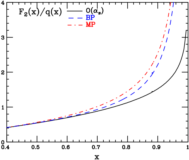
Figure 2: Resummation of the quark coefficient function $C_{2,\,q}^{{\overline{\rm MS}}}\left(Q^{2}/\mu^{2},\alpha(\mu^{2}),N\right)$ for the deep-inelastic structure function $F_{2}$. The resummation is performed up to the next-to-leading logarithmic level matched to the $O(\alpha_{s}(Q^{2}))$ fixed order result. We plot as a function of $x$ the structure function normalized to the parton distribution. The three curves are, top to bottom, the minimal prescription eq. (63), the Borel prescription eq. (65) and the fixed $O(\alpha_{s}(Q^{2}))$ result. We take $\alpha_{s}(Q^{2})=0.2$.

The minimal prescription is then constructed by computing

$$F_{2,q}^{\rm MP}(Q^{2},x)=\int_{C_{\rm MP}}\frac{dN}{2\pi i}x^{-N}\left[C_{2,\,q}^{{\overline{\rm MS}}}\left(1,\alpha(Q^{2}),N\right)+\Sigma(\alpha_{s}(Q^{2}),L)-\Sigma^{\rm NLO}(\alpha_{s}(Q^{2}),L)\right]q(N),$$ (63)

where $C_{\rm MP}$ is the standard minimal prescription contour [6], $\Sigma(\alpha_{s}(Q^{2}),L)$ is the resummed coefficient discussed above, and $\Sigma^{\rm NLO}(\alpha_{s}(Q^{2}),L)$ is its expansion up to order $\alpha_{s}(Q^{2})$, namely

$$\Sigma(\alpha_{s}(Q^{2}),L)-\Sigma^{\rm NLO}(\alpha_{s}(Q^{2}),L)=O\left(\alpha^{2}(Q^{2})\right).$$ (64)

The Borel prescription is constructed computing

$$F_{2,q}^{\rm BP}(Q^{2},x)=\int_{x}^{1}\frac{dy}{y}\left[\bar{C}_{2,\,q}^{{\overline{\rm MS}}}\left(1,\alpha(Q^{2}),y\right)+\bar{\Sigma}(\alpha_{s}(Q^{2}),y)-\bar{\Sigma}^{\rm NLO}(\alpha_{s}(Q^{2}),y)\right]\bar{q}\left(\frac{x}{y}\right),$$ (65)

where $\bar{C}_{2,\,q}^{{\overline{\rm MS}}}\left(1,\alpha(Q^{2}),x\right)$ is the inverse Mellin transform of $C_{2,\,q}^{{\overline{\rm MS}}}\left(1,\alpha(Q^{2}),N\right)$, $\bar{\Sigma}(\alpha_{s}(Q^{2}),x)$ is constructed from $\Sigma(\alpha_{s}(Q^{2}),L)$ using eq. (47) with $R_{B}(x,C)$ given by eq. (45) and (for DIS) $a=1$. We take $C=1$, which corresponds to the inclusion of a twist-four term; the convolution integral in eq. (65) can then be computed with one subtraction eq. (57). Finally, $\bar{\Sigma}^{\rm NLO}(\alpha_{s}(Q^{2}),x)$ is the expansion of $\bar{\Sigma}(\alpha_{s}(Q^{2}),x)$ up to order $\alpha_{s}(Q^{2})$,

$$\bar{\Sigma}(\alpha_{s}(Q^{2}),x)-\bar{\Sigma}^{\rm NLO}(\alpha_{s}(Q^{2}),x)=O\left(\alpha^{2}(Q^{2})\right).$$ (66)

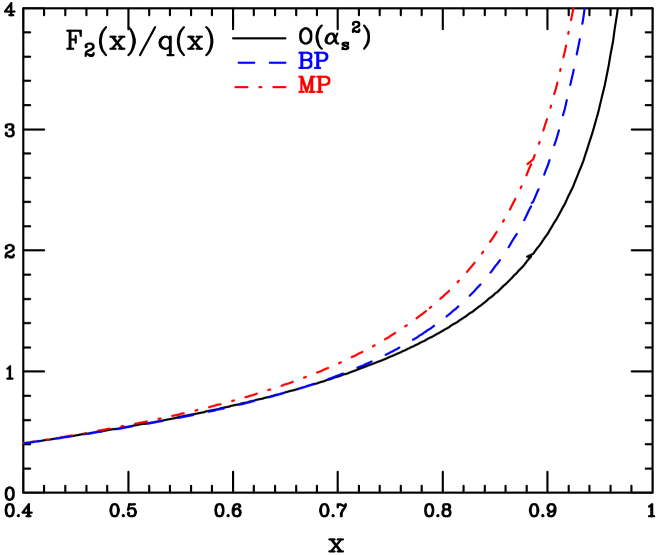
Figure 3: Same as figure 2, but with the resummation performed up to the next-to-next-to-leading logarithmic level and matched to the $O(\alpha_{s}^{2})$ fixed order result.

The results obtained using the MP and the BP are compared to each other and to the fixed $O(\alpha_{s}(Q^{2}))$ result in Fig. 2. The structure function eqs. (63),(65) is plotted as a function of $x$, normalized to the parton distribution eq. (62): namely, we plot $\frac{F_{2,q}(Q^{2},x)}{\bar{q}(x)}$. We take $\alpha_{s}(Q^{2})=0.2$. Note that $\bar{q}(x)$ vanishes very rapidly as $x\to 1$. The comparison shows that the effect of the resummation is sizable for $x\mathrel{\mathchoice{\lower 0.86108pt\vbox{\halign{$\m@th\displaystyle\hfil#$\cr>\crcr\sim\crcr}}}{\lower 0.86108pt\vbox{\halign{$\m@th\textstyle\hfil#$\cr>\crcr\sim\crcr}}}{\lower 0.86108pt\vbox{\halign{$\m@th\scriptstyle\hfil#$\cr>\crcr\sim\crcr}}}{\lower 0.86108pt\vbox{\halign{$\m@th\scriptscriptstyle\hfil#$\cr>\crcr\sim\crcr}}}}0.6$ and becomes of order $100\%$ when $x\mathrel{\mathchoice{\lower 0.86108pt\vbox{\halign{$\m@th\displaystyle\hfil#$\cr>\crcr\sim\crcr}}}{\lower 0.86108pt\vbox{\halign{$\m@th\textstyle\hfil#$\cr>\crcr\sim\crcr}}}{\lower 0.86108pt\vbox{\halign{$\m@th\scriptstyle\hfil#$\cr>\crcr\sim\crcr}}}{\lower 0.86108pt\vbox{\halign{$\m@th\scriptscriptstyle\hfil#$\cr>\crcr\sim\crcr}}}}0.8$, where however $F_{2}(x)$ is very small. Interestingly, while the percentage difference between the MP and BP tends to zero both as $x\to 1$ and $x\to 0$, in the intermediate region $0.6\mathrel{\mathchoice{\lower 0.86108pt\vbox{\halign{$\m@th\displaystyle\hfil#$\cr<\crcr\sim\crcr}}}{\lower 0.86108pt\vbox{\halign{$\m@th\textstyle\hfil#$\cr<\crcr\sim\crcr}}}{\lower 0.86108pt\vbox{\halign{$\m@th\scriptstyle\hfil#$\cr<\crcr\sim\crcr}}}{\lower 0.86108pt\vbox{\halign{$\m@th\scriptscriptstyle\hfil#$\cr<\crcr\sim\crcr}}}}x\mathrel{\mathchoice{\lower 0.86108pt\vbox{\halign{$\m@th\displaystyle\hfil#$\cr<\crcr\sim\crcr}}}{\lower 0.86108pt\vbox{\halign{$\m@th\textstyle\hfil#$\cr<\crcr\sim\crcr}}}{\lower 0.86108pt\vbox{\halign{$\m@th\scriptstyle\hfil#$\cr<\crcr\sim\crcr}}}{\lower 0.86108pt\vbox{\halign{$\m@th\scriptscriptstyle\hfil#$\cr<\crcr\sim\crcr}}}}0.8$ where the resummation is important the two prescriptions lead to rather different results.

We have checked that the replacement of $(1-x)\to\ln\frac{1}{x}$ in the BP has a negligible effect. This ensures that the difference between the MP and BP is not due to a different treatment of non-logarithmically enhanced terms. Furthermore, we have verified that increasing the value of $C$ eq. (24) from one to 1.8 also has essentially no effect. This agrees with expectations based on the results of ref. [7]: there, it was found that $R_{B}(x,C)$ is stable upon variations of $C$ unless $x>x_{L}$ eq. (1), so the same should hold for physical observables where the region of very large $x$ shouldn’t weigh too much. Finally, in Fig. 3 we repeat the same calculation but adding an extra logarithmic order in the resummed result and matching to the fixed order result computed at $O(\alpha_{s}^{2})$. The difference between the fixed–order and resummed results is now smaller, as it ought to be, but the difference between MP and BP has not decreased, thereby showing that this difference is not compensated by the inclusion of higher logarithmic orders.

We must conclude that the difference between the MP and the BP indicates that the ambiguity in the resummation procedure is sizable: a fact which is rather well known in the context of transverse momentum resummation (see e.g. ref. [13]), but not equally obvious for threshold resummation.

In summary, we have presented a new prescription for the resummation of the divergent series of logarithmically enhanced terms which is obtained from threshold resummation. The divergent series is summed through the Borel method, and the divergence in the Borel inversion integral is removed through the inclusion of a suitable higher twist term. This term can be chosen to be of any twist, but the minimal choice is to take it as a twist four contribution. We have described the practical implementation of this prescription and demonstrated its application to the threshold resummation of a deep-inelastic coefficient function, which we have compared to the commonly used minimal prescription.

The Borel prescription and minimal prescription have somewhat complementary advantages and disadvantages: the minimal prescription is naturally implemented in $N$ space, so it is easy to use with $N$–dependent parton distributions. However, in $x$ space the MP leads to partonic cross sections which do not vanish in the unphysical $x>1$ region and its implementation is less straightforward. The Borel prescription directly gives an $x$ space result which has the form of a plus distribution such as found in fixed order perturbative computations. However, its $N$ space form can only be obtained by performing the Mellin transform numerically, and its convolution with a parton distribution must be determined by numerical integration. The Borel prescription also has the advantage that it is possible to control the inclusion of non-logarithmically enhanced terms in the resummation, but it has the disadvantage that it requires the inclusion of higher twist contributions.

Comparison of results obtained using the Borel prescription and the minimal prescription suggests that the ambiguity in threshold resummation is sizable. The extension of this method to the case of resummation of transverse momentum distributions will be presented elsewhere.

Acknowledgement: We thank Paolo Nason for illuminating discussions. S.F. acknowledges partial support from the Marie Curie Research Training Network HEPTOOLS under contract MRTN-CT-2006-035505.

Appendix

In ref. [5] we have determined the Mellin transform of any function of $\ln N$ to all orders in $\ln(1-x)$, up to terms which vanish as $x\to 1$ as a power of $1-x$. However, the exact Mellin transform can also be computed [7]. Indeed, the standard Euler integral representation of the Gamma function implies that

$$\int_{0}^{1}dxx^{N-1}\left[\ln^{\eta-1}\frac{1}{x}\right]_{+}=\Gamma(\eta)\left(N^{-\eta}-1\right).$$ (67)

so

$$\frac{1}{2\pi i}\int_{\overline{N}-i\infty}^{\overline{N}+i\infty}dNx^{-N}N^{-\eta}=\Delta(\eta)\left[\ln^{\eta-1}\frac{1}{x}\right]_{+}+\delta(1-x),$$ (68)

where $\Delta(\eta)\equiv\frac{1}{\Gamma(\eta)}$. It follows that the exact inverse Mellin transform of $\ln^{k}\frac{1}{N}$ is

$$\frac{1}{2\pi i}\int_{\overline{N}-i\infty}^{\overline{N}+i\infty}dNx^{-N}\ln^{k}\frac{1}{N} = \frac{d^{k}}{d\eta^{k}}\left.\frac{1}{2\pi i}\int_{\overline{N}-i\infty}^{\overline{N}+i\infty}dNx^{-N}N^{-\eta}\right|_{\eta=0}$$ (69)

$$= \left.\frac{d^{k}}{d\eta^{k}}\bigg{\{}\Delta(\eta)\left[\ln^{\eta-1}\frac{1}{x}\right]_{+}\right|_{\eta=0}+\delta(1-x)\bigg{\}}$$

$$= \left[\frac{1}{\ln\frac{1}{x}}\sum_{n=1}^{k}\left(\begin{array}[]{c}k\\ n\end{array}\right)n\Delta^{(n-1)}(1)\left(\ln\ln\frac{1}{x}\right)^{k-n}\right]_{+}+\delta_{k0}\delta(1-x),$$ (72)

where in the last step we used $\Delta^{(n)}(0)=n\Delta^{(n-1)}(1).$

References

• [1] S. Catani and L. Trentadue, Nucl. Phys. B 327 (1989) 323.
• [2] G. Sterman, Nucl. Phys. B 281 (1987) 310.
• [3] D. Amati, A. Bassetto, M. Ciafaloni, G. Marchesini and G. Veneziano, Nucl. Phys. B 173 (1980) 429.
• [4] A. V. Manohar, Phys. Rev.  D 68 (2003) 114019;
A. Idilbi, X. d. Ji and F. Yuan, Nucl. Phys.  B 753 (2006) 42;
T. Becher, M. Neubert and B. D. Pecjak, JHEP 0701, 076 (2007).
• [5] S. Forte and G. Ridolfi, Nucl. Phys. B 650 (2003) 229.
• [6] S. Catani, M. L. Mangano, P. Nason and L. Trentadue, Nucl. Phys. B 478 (1996) 273;
• [7] S. Forte, G. Ridolfi, J. Rojo and M. Ubiali, Phys. Lett.  B 635 (2006) 313.
• [8] E. Gardi, G. P. Korchemsky, D. A. Ross and S. Tafat, Nucl. Phys.  B 636 (2002) 385.
• [9] T. O. Eynck, E. Laenen and L. Magnea, JHEP 0306 (2003) 057.
• [10] R. Akhoury, M. G. Sotiropoulos and G. Sterman, Phys. Rev. Lett.  81 (1998) 3819.
• [11] A. Vogt, Phys. Lett.  B 497 (2001) 228.
• [12] W. A. Bardeen, A. J. Buras, D. W. Duke and T. Muta, Phys. Rev.  D 18 (1978) 3998.
• [13] A. Kulesza and W. J. Stirling, JHEP 0312 (2003) 056.