Detecting Directional Selection from the Polymorphism Frequency Spectrum

Abstract

The distribution of genetic polymorphisms in a population contains information about the mutation rate and the strength of natural selection at a locus. Here, we show that the Poisson Random Field (PRF) method of population-genetic inference suffers from systematic biases that tend to underestimate selection pressures and mutation rates, and that erroneously infer positive selection. These problems arise from the infinite-sites approximation inherent in the PRF method. We introduce three new inference techniques that correct these problems. We present a finite-site modification of the PRF method, as well as two new methods for inferring selection pressures and mutation rates based on diffusion models. Our methods can be used to infer not only a “weighted average” of selection pressures acting on a gene sequence, but also the distribution of selection pressures across sites. We evaluate the accuracy of our methods, as well that of the original PRF approach, by comparison with Wright-Fisher simulations.

Introduction

The mutation rate and selection pressures operating on genes are of central importance in shaping their evolution. The number and frequency distribution of genetic polymorphisms within a population carry information about these fundamental processes. Polymorphisms at higher frequencies reflect weaker selective pressures (or positive selection), and vice versa. Similarly, a larger number of polymorphisms indicates a higher mutation rate. Thus we can use the polymorphism frequency spectrum observed in genetic sequences sampled from a population in order to infer the mutation rate and the strength and direction of selection acting on the sequence.

This intuition can be formalized into a rigorous method for estimating selection pressures and mutation rates by calculating the likelihood of sampled polymorphism data as a function of these parameters. The Poisson Random Field (PRF) model provides an important and widely-used method of doing so. The PRF model assumes a panmictic population of constant size, free recombination, infinite sites, no dominance or epistasis, and equal selection pressures at all sites. Under these assumptions, Sawyer and Hartl (1992) showed that the distribution of frequencies of mutant lineages in a population forms a Poisson random field whose properties depend on the selection pressure and the mutation rate. Hartl et al. (1994) and Bustamante et al. (2001) developed a maximum likelihood method of estimating these parameters from data on the polymorphism frequency spectrum. This method has been widely used to study, for example, purifying selection on synonymous Hartl et al. (1994); Akashi and Schaeffer (1997); Akashi (1999) and nonsynonymous Akashi (1999); Hartl et al. (1994) variation, and the evolution of base composition Lercher et al. (2002); Galtier et al. (2006).

Closely related to these analyses of polymorphism data are methods that calculate, based on the PRF model, the ratio of the expected number of polymorphisms within species to divergence between species for synonymous and nonsynonymous sites (using the idea behind the McDonald-Kreitman test McDonald and Kreitman (1991)). These methods discard some of the available data, as they depend only on the number of polymorphisms and not their full frequency spectrum. However, they are also less sensitive to assumptions Loewe et al. (2006); Sawyer and Hartl (1992). Such methods have been applied to estimate selection pressures on synonymous variation Akashi (1995), on nonsynonymous mutations in mitochondrial genomes Nachman (1998); Rand and Kann (1998); Weinreich and Rand (2000), and on nonsynonymous variation in a variety of nuclear genomes Bustamante et al. (2002); Bartolome et al. (2005); Sawyer et al. (2003), including humans Bustamante et al. (2005).

Much recent theoretical work has focused on relaxing various assumptions of the original PRF method. These include allowing for dominance Williamson et al. (2004), population subdivision Wakeley (2003), changing population size Williamson et al. (2005), and linkage between sites Zhu and Bustamante (2005). Several methods for studying the properties of the distribution of selection pressures across sites based on the PRF model have also been developed, both using the polymorphism frequency spectrum Bustamante et al. (2003), and using the ratio of polymorphism to divergence Loewe et al. (2006); Sawyer et al. (2003); Bustamante et al. (2003); Piganeau and Eyre-Walker (2003).

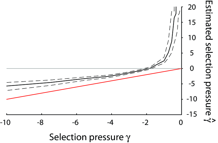
Figure 1: Maximum-likelihood estimates of selection pressures obtained under the PRF method for unfolded polymorphism data. The figure shows the estimated selection pressure $\hat{\gamma}$, on the $y$-axis, obtained by applying the PRF method to $n=14$ sequences sampled from a simulated Wright-Fisher population (see Accuracy of Inference Techniques). Dashed lines indicate the 95% confidence interval around the ML estimate. The true selection pressure $\gamma$ used in the simulations is shown on the $x$-axis. The line $\hat{\gamma}=\gamma$ (i.e. a perfect prediction) is shown in red, and the line $\hat{\gamma}=0$ is shown in gray. The mutation rate is $\theta_{s}=0.5$ per site. The PRF method systematically underestimates the strength of selection, and it often leads to erroneous inferences of strong positive selection when selection is negative. In all cases, the PRF method strongly rejects the true parameters (the difference in the natural log likelihood between $\hat{\gamma}$ and $\gamma$ ranges from 14 to over 700).

All of the methods summarized above fall within the PRF framework, and therefore depend on the infinite-sites approximation. Rather than calculating the evolutionary dynamics at each site, these methods consider the overall steady-state distribution of mutant lineage frequencies across all sites. The PRF method is applied to data by assuming that each lineage segregates at a different site. The infinite-sites assumption is made for purely technical, as opposed to biological, reasons. In this paper, we show that in biologically relevant parameter regimes the infinite-sites assumption causes the PRF method to underestimate selection pressures and mutation rates. This problem arises both for inferences based on the polymorphism frequency spectrum and for inferences based on the ratio of within-species polymorphism to between-species divergence, but in this paper we focus exclusively on the former. As we demonstrate below, the PRF method often underestimates the selection pressure and the mutation rate by as much as an order of magnitude. In addition, and perhaps of greater concern, the PRF method frequently infers that a gene is under strong positive selection when in fact the gene is experiencing weak negative selection (Fig. 1).

In this paper, we present three methods to correct the systematic biases of the PRF method, each with their own advantages and drawbacks. Rather than study mutant lineages across a sequence, our methods all focus on explicit models of the evolutionary dynamics at individual sites. We first present a modification of the PRF method that calculates the frequency distribution of mutant lineages at each site, rather than across the whole sequence. We next present two new methods based on well-known diffusion equations in place of the PRF framework. All three of our methods allow us to estimate the selection pressure and the mutation rate from data on the polymorphism frequency spectrum. In addition, these methods also allow us to infer the distribution of selection pressures across sites. In order to assess the accuracy of these methods, we generate polymorphism data from simulated Wright-Fisher populations with known selection pressures and mutation rates. By comparing inferences drawn from these simulated data sets, we demonstrate that our methods correct the biases inherent in the original PRF approach.

The Poisson Random Field Model of Polymorphisms

We begin by outlining the Poisson Random Field (PRF) model of the site-frequency spectrum developed by Sawyer and Hartl Sawyer and Hartl (1992); Hartl et al. (1994). This model assumes that mutations occur in a population of effective size $N$ at a Poisson rate $Nu$, where $u$ is the per-sequence mutation rate, and are all subject to selection of strength $s$. The fate of each mutant lineage is modeled by a diffusion approximation to the processes of selection and drift. When a new mutant lineage enters the population, it is assumed to arise at a site that has not previously experienced any mutations (the infinite-sites assumption). Each mutant lineage is assumed to be independent of all others (the free-recombination assumption). Since new mutations are continuously arising, and older mutant lineages are fixing or dying out, there is a steady-state distribution of the frequencies of segregating (i.e. non-fixed and non-extinct) mutant lineages. The expected number of segregating sites increases linearly with the mutation rate, but $u$ does not affect the shape of the steady-state distribution of segregating mutant frequencies.

Extending earlier work by Moran (1959) and Wright (1938), Sawyer and Hartl (1992) calculated this steady state distribution of lineage frequencies. They found that the number of lineages with frequency between $x$ and $x+dx$ is Poisson distributed with mean $f(x)dx$, where

$$f(x)=\theta_{l}\frac{1-e^{-2\gamma(1-x)}}{1-e^{-2\gamma}}\frac{1}{x(1-x)}.$$ (1)

Here $\gamma\equiv Ns$ is a measure of the strength of selection on the mutant lineages and $\theta_{l}\equiv 2Nu$ is twice the population per-sequence mutation rate. The function $f(x)$ is referred to as the mean of a Poisson Random Field. In other words, the number of mutant lineages with frequency between $x_{1}$ and $x_{2}$ is a Poisson random variable with mean $\int_{x_{1}}^{x_{2}}f(x)dx$. In addition, the number of mutant lineages with frequency in $[x_{1},x_{2}]$ is independent (as a random variable) from the number of mutant lineages with frequency in $[y_{1},y_{2}]$, provided these intervals do not intersect. Note that $f(x)$ is not integrable at $0$ or $1$. This divergence arises because the steady state is due to a balance between new mutations constantly occurring and older lineages fixing or going extinct. Thus there is no finite, steady-state expression for the number of lineages that have fixed or gone extinct.

Hartl et al. (1994) and Bustamante et al. (2001) used Eq. (1) as the basis for maximum-likelihood (ML) estimation of the mutation rate $\theta_{l}$ and selection pressure $\gamma$ from polymorphism data. They imagined sampling and sequencing $n$ individuals from a population with this steady state distribution of segregating mutant lineages. They made the infinite-sites assumption that all mutant lineages occur at different sites, consistent with the earlier assumption that each lineage is independent (used to derive Eq. (1)). If a given site has a mutant lineage at frequency $x$ in the entire population, then the probability that a sample of $n$ individuals will contain $i$ mutant nucleotides and $n-i$ ancestral nucleotides at the site is ${n\choose i}x^{i}(1-x)^{n-i}$. That is, for each mutant lineage with frequency $x$, there is a probability ${n\choose i}x^{i}(1-x)^{i}$ of finding a corresponding site with $i$ mutant nucleotides. Since the number of mutant lineages at frequency $x$ in the population is Poisson distributed with mean $f(x)dx$, the number of sampled sites containing $i$ mutant nucleotides (we refer to these as $i$-fold mutant sites) is Poisson distributed with mean

$$F(i)=\theta_{l}\int_{0}^{1}\frac{1-e^{-2\gamma(1-x)}}{1-e^{-2\gamma}}\frac{1}{x(1-x)}{n\choose i}x^{i}(1-x)^{n-i}dx.$$ (2)

This equation leads immediately to a maximum likelihood procedure for estimating $\gamma$ and $\theta_{l}$ Bustamante et al. (2001). A set of sequences from $n$ sampled individuals within a population will contain some number, $y_{i}$, of $i$-fold mutant sites for $0<i<n$. The set of values $y_{1}$, $y_{2}$, $\ldots$ $y_{n-1}$ is called the site-frequency spectrum of the observed data. The probability of a spectrum $\{y_{i}\}$, given $\gamma$ and $\theta_{l}$, is

$$L_{u}(\theta_{l},\gamma)=\prod_{i=1}^{n-1}e^{-F(i;\gamma,\theta_{l})}\frac{\left[F(i;\gamma,\theta_{l})\right]^{y_{i}}}{y_{i}!}.$$ (3)

For an observed spectrum $y_{i}$ in a particular data set, we can maximize this likelihood over $\theta_{l}$ and $\gamma$ to estimate the mutation rate and selection pressure.

The likelihood expression above assumes we know which nucleotide is ancestral and which nucleotide is the mutant at each polymorphic site. We refer to this situation as the unfolded case. When we do not have this information, we cannot distinguish between an $i$-fold mutant site and an $(n-i)$-fold mutant site. In this case, a data set will contain some number, $y_{i}$, $i$-fold and/or $(n-i)$-fold mutant sites, where $i$ runs between $1$ and the largest integer less than or equal to $n/2$. We refer to this as the folded case. In this situation, the likelihood of a particular data set $L_{f}(\theta_{l},\gamma)$ is given by the same expression as in $L_{u}$, but with the product running from $1$ to $n/2$ and with $F(i)$ replaced by $F(i)+F(n-i)$ (except if $i=n/2$).

Shortcomings of the Poisson Random Field model

The PRF model makes two key assumptions: that each site is independent of all the others, and that two mutant lineages never segregate at the same site. The former assumption is equivalent to assuming free recombination between all sites which segregate concurrently. This assumption may be violated in many populations, particularly when the method is applied to estimate selective pressures on short stretches of DNA (e.g. a single gene) that are linked over long timescales. Ideally, we would like a theory that allows us to infer the strength of selection acting on a large number of sites with an arbitrary degree of linkage, but no such theory yet exists. Nevertheless, a free recombination model is useful as a null model and a limiting case, and it can be used to compare with more complicated possibilities. Such a model may also be used to test whether recombination is necessary to explain data from a particular population. Furthermore, whenever selection pressures are weak, sites segregate over long timescales and so recombination may be frequent enough that even intragenic sites are unlinked over these timescales. Finally, it is important to note that linkage between segregating sites will not bias estimates of the selection pressure, provided it is equal across sites, but rather increase the variance in such estimates Bustamante et al. (2001); Akashi and Schaeffer (1997).

The second assumption of the PRF, that there are an infinite number of sites, is more problematic. This problem is most apparent when considering how the PRF method treats “multiply polymorphic” sites — those that exhibit more than two types of segregating nucleotides. We refer to the configuration of a particular site as $(a,b,c,d)$, where $a$, $b$, $c$, and $d$ are the numbers of sampled sequences which exhibit each of the four nucleotides. When we have unfolded data, $a$ is the frequency of the ancestral nucleotide and $b$, $c$, and $d$ are the frequencies of the three possible mutant nucleotides, in order of decreasing frequency. When we have folded data, $a$, $b$, $c$, and $d$ are the frequencies of all four possible nucleotides, again in order of decreasing frequency. In the original PRF analysis, a site with a $(12,1,1,0)$ configuration, for example, is treated identically to a site with a $(12,2,0,0)$ configuration. Such a treatment is incorrect: the former configuration can only arise from two low-frequency mutant lineages, whereas the latter configuration could be caused by a single high-frequency lineage. Yet the PRF analysis excludes the first possibility, and treats both configurations as if they were all $(12,2,0,0)$ sites Hartl et al. (1994); Bustamante et al. (2001). Similarly, the PRF method treats $(10,2,2,0)$, $(10,3,1,0)$, and $(10,2,1,1)$ sites as if they were in a $(10,4,0,0)$ configuration, etc.

The infinite sites approximation also affects sites that are not multiply polymorphic. The essential problem is that the sampling mechanism used to calculate $F(i)$ under the PRF method implicitly assumes that each mutant lineage occurs at a different site. The number of $i$-fold mutant sites is assumed to equal the number of $i$-fold mutant lineages sampled. Yet if multiple lineages are segregating at the same site, an $i$-fold and a $k$-fold mutant lineage sampled at the same site can lead to an apparently $(i+k)$-fold mutant site, if the two lineages happen to be mutations to the same nucleotide. In other words, a $(12,2,0,0)$ site could reflect two low-frequency mutant lineages or one higher-frequency one, but the PRF incorrectly assumes that only the latter is possible.

The infinite-sites assumption is problematic whenever there are multiple mutations segregating at a site, even if they are at low frequency. Since a mutant lineage will survive on average $O(\ln\left[1/|s|\right])$ generations before fixing or going extinct, and mutations arise at rate $N\mu$ per site, the infinite-sites approximation will be valid only when $N\mu\ln\left[1/|s|\ll\right]1$. This condition is often violated in real populations. In fact, several estimates of mutation rates and selective pressures based on the PRF method violate this condition Hartl et al. (1994). We can also see explicitly that this condition is violated whenever a data set includes multiply polymorphic sites. Polymorphisms of this type are indeed observed in data analyzed by PRF method Hartl et al. (1994).

Unlike the assumption of free recombination, the assumption of infinite sites is purely technical. In other words, we do not aspire to use the PRF method as a null model for exploring whether or not real systems violate the infinite sites assumption. This assumption is highly problematic because it induces systematic biases in the estimates of selection and mutation obtained by the PRF method: the method always treats an $i$-fold sampled site as having arisen from a single mutant lineage that has reached frequency $i$ in the sample, ignoring the possibility of multiple mutant lineages at lower frequencies which sum to $i$. By disregarding the latter possibilities, the PRF method systematically underestimates the mutation rate $u$ and the strength of selection $|s|$. Even though sites that violate the infinite sites approximation may be very rare, they have a disproportionate weight in estimates of these parameters and thus can lead to errors of an order of magnitude or more (see below). The method also erroneously infers positive selection in many situations where selection is actually negative. Both of these problems arise across a broad and biologically relevant range of parameters (Fig. 1).

In addition to the systematic biases in the estimates it produces, the PRF method also wastes data. In particular, it makes no use of the information contained in the monomorphic sites of a sample. Given a $\gamma$ and $\theta_{l}$, the PRF method predicts the number of sites $y_{i}$ that will exhibit $i$-fold polymorphisms, for $i$ between $1$ and $n$, the sample size. The PRF method makes no prediction about the number of monomorphic sites (more precisely the infinite sites approximation assumes that there is an infinite set of monomorphic sites among which the polymorphism is found). Thus if we had two sets of sequences with the same configuration of polymorphic sites but different numbers of monomorphic sites, ML estimation based on the PRF method would infer identical (per-sequence) mutation rates and selective coefficients. This holds despite the fact that monomorphic sites certainly contain information: a larger number of monomorphic sites reflects a lower mutation rate or stronger selection or both.

Two other assumptions of the PRF model are worth mentioning. First, the PRF method assumes that all sites experience the same selective pressure. In practice, this means that the PRF estimate of the selection strength $s$ is actually some sort of weighted average of the selective forces acting on the sites analyzed. For example, since any site with $|s|\gg\frac{1}{N}$ will almost always be monomorphic, and data on monomorphism is ignored, such sites will not influence the PRF ML estimate of the “average” $s$. But beyond this, the weighting in this average is unclear, and hence it is unclear what the PRF ML estimate of $s$ really represents. We explore this issue of variable selective pressures in more detail below.

Finally, the PRF framework assumes that, once a mutation fixes at a particular site, additional mutations at the site will experience the same selective coefficient as the original mutation. For example, if a mutation from nucleotide $A$ to $C$ fixes despite a selective disadvantage $s$, new mutations at this site (e.g. from $C$ back to $A$) are assumed to again have selective disadvantage $s$. This unrealistic assumption arises because the PRF focuses on a steady state distribution of mutant lineages without references to the sites at which they occur — the fixation of old mutants is simply assumed to balance the continuous generation of new ones, but not to change the selective advantage of future mutations. There is no reference to the evolutionary dynamics at individual sites. Although unrealistic for negative selection, this approach has some advantages. In particular, it makes modeling positive selection straightforward: positive selection is simply a constant flux of new mutations that increase the fitness, and a steady state distribution of their frequencies is well defined.

A Per-Site Poisson Random Field Model of Polymorphisms

The problems with the PRF method described above can all be resolved by replacing it with an explicit model of evolution at each site. We develop such a model in the following section. First, however, we describe in this section a method that retains the basic PRF framework, but corrects some of the problems associated with the infinite-sites assumption, and takes full advantage of the information provided by the frequencies of all possible configurations at a site.

The basic idea behind this modified approach is to recast the PRF framework on a per-site basis. We describe the steady state frequency distribution of mutant lineages at a given site. From this, we can calculate the probability that a sample of $n$ individuals will contain any configuration of mutants at that site. As in the original PRF method, we retain the assumption of free recombination, so that the DNA sequence is a collection of independent sites. Thus our per-site analysis leads directly to ML estimation of mutation rate and selection strength.

We begin by recasting the PRF expression for the steady state distribution of mutant lineages to describe the frequencies of mutant lineages at a single site. At a given site, we have

$$f(x)=\theta_{s}\frac{1-e^{-2\gamma(1-x)}}{1-e^{-2\gamma}}\frac{1}{x(1-x)},$$ (4)

where $\theta_{s}$ is the per-site value, $\theta_{s}=2N\mu$. Using this formula to describe multiple lineages at a single site is somewhat peculiar, because this result assumes that all mutant lineages behave independently of one another. Clearly this is not strictly true, since the mutant lineages are segregating at the same site. However, provided two mutant lineages rarely achieve simultaneous high frequencies in the population, then the assumption of independent mutant lineages is a good approximation. This assumption of non-interacting mutant linages will often hold even when the other aspects of the infinite-sites approximation are violated.

Analogous to the original PRF method, at a single site the number of mutant lineages which are observed $i$ times in a sample of $n$ sequences (“$i$-fold mutant lineages”) is Poisson distributed with mean

$$F(i)=\theta_{s}\int_{0}^{1}\frac{1-e^{-2\gamma(1-x)}}{1-e^{-2\gamma}}\frac{1}{x(1-x)}{n\choose i}x^{i}(1-x)^{n-i}dx.$$ (5)

Based on this, we can calculate the probability of any particular polymorphism configuration at a site.

We begin by describing this calculation in the unfolded case. The probability that a site is monomorphic is just the probability that no $i$-fold mutant lineages are found at that site, for all $i$ between $1$ and $n-1$. This is

$$P_{mono}=P_{(n,0,0,0)}=e^{-F(1)}e^{-F(2)}\ldots e^{-F(n-1)}\equiv M.$$ (6)

The probability that a site exhibits a $(n-1,1,0,0)$ configuration is the probability that a single $1$-fold mutant lineages is sampled, and no $2$-fold or higher lineages are found,

$$P_{(n-1,1,0,0)}=F(1)M.$$ (7)

The probability of exhibiting an $(n-2,2,0,0)$ configuration is more complex. This configuration could arise from a single $2$-fold sampled lineage (as assumed under the standard PRF method) or it could arise from two $1$-fold sampled mutant lineages which happen to involve mutations to the same nucleotide. Hence its probability is

$$P_{(n-2,2,0,0)}=\frac{F(1)^{2}}{2!}M\frac{1}{3}+F(2)M,$$ (8)

where the factor of $\frac{1}{3}$ is the probability that two mutations result in the same nucleotide. This expression assumes that mutations between all possible nucleotides are equally likely — the obvious generalization applies when there are mutational biases, which we do not discuss further. Similarly the probability of an $(n-2,1,1,0)$ configuration is

$$P_{(n-2,1,1,0)}=\frac{F(1)^{2}}{2!}M\frac{2}{3}.$$ (9)

The probabilities of more complex configurations can be calculated in a similar way. The probability of an $(n-4,4,0,0)$ configuration, for example, is the probability of four $1$-fold lineages to the same nucleotide plus the probability of two $1$-fold lineages and a $2$-fold lineages, plus the probability of two $2$-fold lineages, plus the probability of one $1$-fold lineage and one $3$-fold lineage, plus the probability of a single $4$-fold lineage. We have

$$P_{(n-4,4,0,0)}=M\left[\frac{F(1)^{4}}{4!}\frac{1}{3^{3}}+\frac{F(1)^{2}F(2)}{2!}\frac{1}{3^{2}}+\frac{F(2)^{2}}{2!}\frac{1}{3}+F(1)F(3)\frac{1}{3}+F(4)\right].$$ (10)

In general, the probability of a particular configuration is given by the sum of the probabilities of all possible partitions of $n$ that lead to that configuration.

In the folded case, these calculations become even more complex. The probability of a $(12,2,0,0)$ folded configuration, for example, includes the probability of a single $12$-fold sampled lineage, as well as two $6$-fold sampled lineages, and so on. Thousands of terms may arise in the expression for the probability of a particular configuration, even for moderate values of $n$. We do not quote any of these results here, but rather we have developed a computer program to output symbolic expressions for the probabilities of all possible folded as well as unfolded configurations, for a given sample size $n$ (available on request).

These probabilities of site configurations form the basis of maximum likelihood parameter estimation. The probability of a data set with $L$ total sites, including $L_{a,b,c,d}$ sites in configuration $(a,b,c,d)$ is given by

$$\frac{L!}{\prod L_{a,b,c,d}!}\prod P_{a,b,c,d}^{L_{a,b,c,d}},$$ (11)

where the products are over all possible configurations. Given a particular data set, we maximize this probability over $\theta_{s}$ and $\gamma$ to find the ML estimate of these parameters. In the original PRF method, this ML estimation is particularly simple, because the ML estimate for $\theta$ can be expressed analytically in terms of the ML estimate for $\gamma$, leaving a one-dimensional numerical maximization procedure to estimate $\gamma$. In our per-site PRF method, however, a full two-dimensional numerical maximization is required to find the ML estimates of $\theta_{s}$ and $\gamma$.

Our per-site PRF method relaxes most of the consequences of the infinite-sites approximation inherent in the original PRF estimation procedure. We allow for the possibility that multiple mutant lineages contribute to the polymorphism observed at a single site. Thus we avoid the systematic underestimation of $\theta$ and $\gamma$, and incorrect inference of positive selection, that affect the traditional PRF (see Numerical Simulations). This new method also uses all of the data available in the sample, including the number of monomorphic sites and the differences between $(n-2,2,0,0)$ and $(n-2,1,1,0)$ sites. It does still retain one aspect of the infinite-sites approximation: it assumes that mutant lineages segregating at the same site are independent (i.e. they do not interfere with each other). This is never strictly true, but is a good approximation unless multiple mutant lineages reach high frequency at a given site at the same time. Note that because of this assumption, the probabilities of all possible configurations $(a,b,c,d)$ described above do not precisely sum to unity, because our approach allows a typically small but nonzero probability of multiple mutant processes adding to more than $n$ sampled individuals. Since the no-interference approximation is always valid when the infinite-sites approximation is, and it holds in many situations where the infinite-sites approximation fails, our revised sampling method extends the applicability of the PRF framework and fixes many of its problems.

A Per-Site Diffusion Model of Polymorphisms

In this section, we describe a method that shifts fundamentally from the PRF framework. Rather than studying the distribution of the frequencies of mutant lineages, we focus on the evolutionary dynamics at each individual site, without keeping track of individual mutant lineages. We develop this into a maximum-likelihood estimation of $\gamma$ and $\theta$ from polymorphism data, which requires neither the infinite-sites or no-interference approximation described above. As in the original PRF method, we assume free recombination between sites.

At an individual site, we imagine that one nucleotide is preferred, and the other three have the same fitness disadvantage $s$ ($s<0$). We assume that mutations occur at rate $\mu$, and hence at rate $\mu/3$ between any two specific nucleotides (i.e. no mutational biases). These assumptions simplify the discussion, but are not essential. In fact, one advantage of this approach is that these assumptions can be easily relaxed with obvious generalizations (noted below).

We can analyze the process of mutation, selection, and drift at a single site with a three-dimensional diffusion approximation, and calculate the joint steady-state probability distribution of the frequencies of the four possible nucleotides at the site. This then leads naturally to the likelihood of any configuration of polymorphism data at the site as a function of $\gamma$ and $\theta_{s}$, and hence to a ML estimation of these parameters from data. Alternatively, we can sacrifice some of the information in the data, and reduce the computational complexity of the problem by treating all three disfavored nucleotides as a single class. Such a treatment reduces to a standard one-dimensional diffusion process whose steady state probability distribution describes the frequency of the preferred nucleotide versus the sum of the frequencies of the disfavored ones; this treatment is essentially a steady-state version of Williamson et al. (2005). This approach discards some of the information in the data (e.g. not making use of the difference between $(12,1,1,0)$ and $(12,2,0,0)$ sites), but it is computationally simpler. We begin by describing the one-dimensional method, and then turn to the three-dimensional method.

The One-Dimensional Diffusion Model

We begin by describing a simplified diffusion approach that calculates the frequency distribution of favored versus disfavored nucleotides. As noted above, we will for simplicity assume that one nucleotide is preferred, and the other three nucleotides are disfavored. We denote the sum of the frequencies of the three disfavored alleles by $x$; the frequency of the preferred nucleotide is $1-x$.

We assume that mutation, selection, and random drift occur at each site according to standard Wright-Fisher dynamics. Thus the probability distribution of $x$ can be described by the diffusion equation

$$\frac{\partial{}}{\partial{t}}f(x,t)=\frac{1}{2}\frac{\partial^{2}}{\partial x^{2}}\left[v(x)f(x,t)\right]+\frac{\partial{}}{\partial{x}}\left[m(x)f(x,t)\right],$$ (12)

where $f(x,t)$ is the probability that the disfavored nucleotides sum up to frequency $x$ at time $t$, $s$ is the selection coefficient against the disfavored nucleotides ($s<0$), $\mu$ is the per-site mutation rate per individual per generation, and

$$m(x) = sx(1-x)+\mu(1-x)-\frac{\mu}{3}x$$ (13)

$$v(x) = \frac{x(1-x)}{N}.$$ (14)

This diffusion equation is well-known and has the steady-state solution

$$f(x)=Cx^{\theta_{s}-1}(1-x)^{\theta_{s}/3-1}e^{2\gamma x},$$ (15)

where $C$ is a ($\theta_{s}$ and $\gamma$-dependent) normalization factor, and as before $\theta_{s}\equiv 2N\mu$ and $\gamma\equiv Ns$.

If the frequency of disfavored nucleotides at a site equals $x$, the probability that we find $i$ such nucleotides in a sample of $n$ individuals is ${n\choose i}x^{i}(1-x)^{n-i}$. Averaging over $x$, the overall probability that we sample $i$ disfavored nucleotides at a given site is

$$F(i)={n\choose i}\int_{0}^{1}Cx^{\theta_{s}+i-1}(1-x)^{\theta_{s}/3+n-i-1}e^{2\gamma x}\ \text{d}x.$$ (16)

This integral, including the calculation of the normalization factor $C$, can be solved analytically. We find

$$F(i)={n\choose i}\frac{\Gamma(n-i+\theta_{s}/3)\Gamma(i+\theta_{s}){}_{1}F_{1}(i+\theta_{s},n+4\theta_{s}/3,2\gamma)}{\Gamma(\theta_{s}/3)\Gamma(\theta_{s}){}_{1}F_{1}(\theta_{s},4\theta_{s}/3,2\gamma)},$$ (17)

where $\Gamma$ is Euler’s Gamma function and ${}_{1}F_{1}$ is a hypergeometric function.

The expression above leads immediately to a maximum likelihood method for estimating $\gamma$ and $\theta_{s}$ in the unfolded case – i.e. when the identity of the preferred nucleotide at each site is known. In a sample of $n$ sequences each of length $L$, we count the number of sites at which $i$ disfavored nucleotides are sampled, $y_{i}$, for $0\leq i\leq n$. Since all sites are assumed independent, each with the polymorphism frequency distribution described above, the likelihood of the data given the parameters is

$$y_{u}(\theta_{s},\gamma)=\frac{L!}{\prod_{i=0}^{n}y_{i}!}\prod_{i=0}^{n}F(i)^{y_{i}}.$$ (18)

For any set of polymorphism data, it is straightforward to maximize this function numerically, producing ML estimates of $\theta_{s}$ and $\gamma$. As with the per-site PRF method, this procedure involves a two-dimensional maximization routine.

When we do not know which nucleotide is preferred at each site, we must use the “folded” version of the data. This presents difficulties. Imagine a site with an $(a,b,c,d)$ polymorphism configuration. We might naively suppose that since any of the four nucleotides could be the preferred one, the probability of this data is simply $F(b+c+d)+F(a+c+d)+F(a+b+d)+F(a+b+c)$. However, this is not the case. For example, if $a$ is indeed the preferred nucleotide, then $F(b+c+d)$ does not equal the probability that the three disfavored nucleotides will form a $(b,c,d)$ configuration. Rather, it equals the sum of the probabilities that the three disfavored nucleotides will form a configuration $(i,j,k)$, summed over all $i,j,k$ triplets that sum to $b+c+d$. This is a serious problem, because the difference between $F(b+c+d)$ and the probability of the data depends on $b+c+d$, and hence it is not identical for all four possible preferred nucleotides. Simply assuming that the most common nucleotide is the preferred one Hartl et al. (1994) is a reasonable approach to folded fits. But this approach will be inaccurate for sites where the most common nucleotide is not overwhelmingly so; when this situation describes a substantial fraction of sites, the method will fail. As a result, the one-dimensional diffusion framework does not allow for a rigorous ML estimate of parameters with folded data. The exact same problem also arises in the traditional PRF method, although it tends to be obscured by the other problems with that method.

In order to perform rigorous ML fits to folded frequency data we must turn to a three-dimensional diffusion method, which we will now discuss.

The Three-Dimensional Diffusion Model

Rather than considering all disfavored nucleotides as a single class, we can instead keep track of the evolutionary dynamics of all four possible nucleotides at a site. In order to do so, we assume the standard four-allele Wright-Fisher dynamics, with mutation at rate $\frac{\mu}{3}$ between any two particular nucleotides, and selection acting with strength $s$ against the three disfavored nucleotides. The dynamics can then be described by a three-dimensional diffusion equation for the joint distribution of the frequencies of the three disfavored alleles $x_{1},x_{2}$, and $x_{3}$, $f(x_{1},x_{2},x_{3},t)$ (where the preferred allele has frequency $x_{0}=1-x_{1}-x_{2}-x_{3}$). We have

$$\frac{\partial{}}{\partial{t}}f(x_{1},x_{2},x_{3},t)=\frac{1}{2}\sum_{i=1}^{3}\sum_{j=1}^{3}\frac{\partial^{2}}{\partial x_{i}\partial x_{j}}\left[V_{ij}\cdot f\right]-\sum_{i=1}^{3}\frac{\partial{}}{\partial{x_{i}}}\left[M_{i}\cdot f\right],$$ (19)

where

$$M_{i} = (1+s)x_{i}\left(1-\sum_{j=1}^{3}x_{j}\right)+\frac{\mu(1-4x_{i})}{3}$$ (20)

$$V_{ii} = \frac{x_{i}(1-x_{i})}{N}$$ (21)

$$V_{ij} = -\frac{x_{i}x_{j}}{N}\ \ \ \ \ \ \ \ \ (i\neq j).$$ (22)

This is a somewhat less well-known diffusion equation Watterson (1977); Wright (1949); the steady-state solution is

$$f(x_{1},x_{2},x_{3})=C\left[x_{1}x_{2}x_{3}(1-x_{1}-x_{2}-x_{3})\right]^{\zeta}e^{2\gamma\left(x_{1}+x_{2}+x_{3}\right)},$$ (23)

where $C$ is a normalization factor, and we have defined $\zeta=\theta_{s}/3-1$.

Given the frequencies $x_{0}$, $x_{1}$, $x_{2}$, and $x_{3}$ of nucleotides in the population, the probability of sampling a site in an unordered configuration $(n_{0},n_{1},n_{2},n_{3})$ in a sample of $n$ individuals (adopting the convention that the first nucleotide listed is the preferred one) is just the multinomial probability

$$\frac{n!}{n_{0}!n_{1}!n_{2}!n_{3}!}(1-x_{1}-x_{2}-x_{3})^{n_{0}}x_{1}^{n_{1}}x_{2}^{n_{2}}x_{3}^{n_{3}}.$$ (24)

Averaging over $f$, we therefore find that the probability of sampling a site in an unordered $(n_{0},n_{1},n_{2},n_{3})$ configuration is

$$P_{n_{0},n_{1},n_{2},n_{3}} = C\frac{n!}{n_{0}!n_{1}!n_{2}!n_{3}!}\int_{0}^{1}\int_{0}^{1-x_{1}}\int_{0}^{1-x_{1}-x_{2}}\times$$ (26)

$$e^{2\gamma\left(x_{1}+x_{2}+x_{3}\right)}x_{1}^{\zeta+n_{1}}x_{2}^{\zeta+n_{2}}x_{3}^{\zeta+n_{3}}\left[1-x_{1}-x_{2}-x_{3}\right]^{\zeta+n_{0}}dx_{3}dx_{2}dx_{1}.$$

In some applications, we will know which of the nucleotides is preferred at each site — i.e. the unfolded case. In this case, the probability of finding a site in an ordered unfolded configuration $(a,b,c,d)$ (where by convention $a$ is the number of individuals which have the preferred nucleotide and $b\geq c\geq d$), is

$$P^{u}_{a,b,c,d}=\sum_{\{n_{0},n_{1},n_{2},n_{3}\}}P_{n_{0},n_{1},n_{2},n_{3}},$$ (27)

where the sum is over all unordered configurations $(n_{0},n_{1},n_{2},n_{3})$ that give rise to the ordered unfolded configuration $(a,b,c,d)$.

In other cases, we do not know which of the nucleotides is preferred at each site – i.e. the folded case. Here, the probability of sampling a site in the ordered configuration $(a,b,c,d)$ is just the sum of the probabilities assuming that each of the four possible nucleotides is preferred. As before, we adopt the convention that ordered folded configurations are written as $(a,b,c,d)$ with $a\geq b\geq c\geq d$. The probability of a folded configuration $P^{f}_{a,b,c,d}$ is then

$$P^{f}_{a,b,c,d}=\sum_{\{n_{0},n_{1},n_{2},n_{3}\}}P_{n_{0},n_{1},n_{2},n_{3}},$$ (28)

where in this case the sum is over all unordered configurations that give rise to the ordered folded configuration $(a,b,c,d)$.

For either folded or unfolded data, given $n$ samples of a sequence $L$ sites long, with $L_{a,b,c,d}$ sites in an $(a,b,c,d)$ polymorphism configuration, the likelihood of the data is

$$L(\theta_{s},\gamma)=\frac{L!}{\prod L_{a,b,c,d}!}\prod\left[P_{a,b,c,d}\right]^{L_{a,b,c,d}},$$ (29)

where the products are taken over all possible configurations $(a,b,c,d)$ and $P_{a,b,c,d}$ is the folded or unfolded probability defined above. We can numerically maximize this function to find the ML estimates of $\theta_{s}$ and $\gamma$.

In practice, the ML estimation procedure described above is difficult to implement, because of the triple integral in the definition of $P_{n_{0},n_{1},n_{2},n_{3}}$ (as well as that implicit in the definition of the normalization constant $C$). This integral cannot be solved exactly, and it is difficult to evaluate numerically because the integrand may diverge (though the integral itself converges) near the boundary of the simplex over which it is integrated. We adopt a hybrid method to simplify the evaluation of this triple integral. Near the boundary of the simplex, we Taylor expand the integrand and integrate it analytically. Away from the boundary, the integrand is well-behaved and standard numerical integration has no difficulties. This approach is most easily achieved by making the substitutions $y=x_{3}/(1-x_{1}-x_{2})$ and $z=x_{2}/(1-x_{1})$. On doing so, we can rewrite the integral as

$$P_{n_{0},n_{1},n_{2},n_{3}} = C\frac{n!}{n_{0}!n_{1}!n_{2}!n_{3}!}\int_{0}^{1}\int_{0}^{1}\int_{0}^{1}\times$$

$$\exp\left[2\gamma\left(x+y+z-xy-zy-xz+xyz\right)\right]x^{n_{1}+\zeta}z^{n_{2}+\zeta}y^{n_{3}+\zeta}\times$$

$$\left(1-x\right)^{n_{0}+n_{2}+n_{3}+3\zeta+2}\left(1-z\right)^{n_{0}+n_{3}+2\zeta+1}\left(1-y\right)^{n_{0}+\zeta}.$$

This expression is much easier to handle than our original expression, because the three integrals can be done in arbitrary order. We divide each of the three integrals into three pieces: one from $0$ to $\delta$, one from $\delta$ to $1-\delta$, and one from $1-\delta$ to $1$. Thus the triple integral is split into $27$ total terms. For each of the integrals from $0$ to $\delta$ or $\delta$ to $1-\delta$, we Taylor expand the integrand in the integration variable, and we solve the integral analytically. All of the remaining integrals, from $\delta$ to $1-\delta$, are done numerically. We must choose $\delta$ large enough that we can perform the numerical integrals quickly, but not so large that the Taylor expansions used for the analytical parts become invalid. For these Taylor expansions, we need $\delta\ll\frac{1}{2\gamma}$, $\delta\ll 1$, $\delta\ll\frac{1}{3\zeta+2}$, $\delta\ll\frac{1}{2\zeta+1}$, and $\delta\ll\frac{1}{\zeta}$. For the computational analysis described in this paper, we choose whichever of these conditions is most restrictive and set $\delta$ to be one-tenth of the most restrictive requirement. We find that this choice of $\delta$ is sufficiently small to provide accuracy in the analytical parts of the integrals, but large enough to enable quick numerical integration on the interior of the simplex.

Comparison between the PRF and diffusion methods

Both our one- and three-dimensional diffusion approaches relax all of the infinite-sites assumptions of the PRF framework. This includes the interference between mutant lineages segregating at the same site, which even the per-site PRF method mishandles. Thus, the diffusion approach contains none of the biases associated with infinite-sites approximation that plague the traditional PRF and, to a lesser degree, the per-site PRF. The diffusion approach also provides a clear and concrete model of the evolution at each site. This contrasts with the PRF method, which makes the unrealistic assumption that if a deleterious allele fixes at a site, further mutations are again deleterious.

The diffusion method is also easily extendable to more complex evolutionary situations. For example, we can explore different selective costs for different nucleotides, more than one preferred nucleotide, or mutational biases. These possibilities lead to obvious modifications of the diffusion equations and their solutions, and hence to the maximum likelihood estimation. It is also straightforward to investigate balancing selection or the effects of dominance: these lead to well-understood modifications to the diffusion equations and their steady state solutions Ewens (2004). In the PRF framework, by contrast, such generalizations are much more complex. In particular, balancing selection is impossible to analyze under the PRF framework, because it leads to mutant lineages reaching stable intermediate frequencies in the population. As a result, the generation of new mutations is not balanced by the extinction or fixation of older ones, and hence no steady state distribution of lineage frequencies exists.

However, the diffusion approach is not without drawbacks. The one-dimensional version does not make use of all of the data available in the observed polymorphism spectrum. The three-dimensional version does use all the data, but its implementation requires tedious numerical integration routines.

The diffusion method also cannot naturally handle positive selection. The steady state evolutionary dynamics at a site are always dominated by the preferred nucleotide (or nucleotides), with negative selection acting against polymorphisms for the disfavored nucleotides. At the level of an individual site, positive selection is a process that is intrinsically out of steady state: the spread of a favorable nucleotide before it becomes fixed. The PRF method handles this by positing that there are a wide array of sites which have the potential for positive selection, and assuming that a steady state across sites of these selective sweeps is maintained. It should be possible to address positive selection within the diffusion framework by changing the boundary conditions of our diffusion equations, so that the fixation of one mutant lineage shifts the selective landscape so that further mutations are now favored. Formally, any probability flowing into $x=1$ is “absorbed” and moved to $x=0$. Alternatively, one could use full time-dependent solutions to the diffusion equations to study positive selection. However, we do not pursue these approaches in this paper, and instead focus our study on the case of negative selection.

Variable selection pressures across sites

Both the original PRF method as well as the three per-site methods we have proposed in this paper assume that all sites experience the same selective pressure. In reality, we expect that there is some distribution of selective pressures across sites. Hartl et al. (1994) suggest that in this case the ML estimate of $\gamma$ from their PRF method reflects an “average” selection pressure across the sites. In fact, the ML $\gamma$ reflects a weighted average of the actual $\gamma$’s across the sites, but the nature of this weighting is not understood. Almost no weight is given to sites at which $|\gamma|\gg 1$, because these sites will almost always be monomorphic and hence ignored by the original PRF method. It is unclear how sites with different values of $\gamma$ of order $1$ will be weighted, or how the presence of some effectively neutral sites ($|\gamma|\ll 1$) will change the ML estimate.

The issue of variable $\gamma$ across sites is of even greater concern for the methods we have proposed, because these methods make use of the monomorphism data. If some number $L_{l}$ sites are effectively lethal (i.e. $|\gamma|\gg 1$), these sites will increase the number of monomorphic sites, which will tend to depress our ML estimate of $\theta_{s}$ and increase our estimate of $|\gamma|$. Fortunately, our methods are able to use the monomorphism data in order to investigate the number of lethal sites, $L_{l}$, or more generally to infer a full distribution of selection pressures across sites.

Since all of the methods we have proposed are defined at a per-site level, it is straightforward to assume that there are multiple different classes of sites with different values of $\gamma$. We can posit that there are $k$ classes of sites. Each class is represented by $L_{k}$ of $L$ total sites, and has its own value of $\gamma$, which we call $\gamma_{k}$. The probability that a site is in an $(a,b,c,d)$ configuration is then

$$P_{a,b,c,d}=\sum_{j=1}^{k}\frac{L_{j}}{L}P_{a,b,c,d}^{j}(\gamma_{j},\theta_{s}),$$ (31)

where $P_{a,b,c,d}^{j}(\gamma_{j},\theta_{s})$ is the probability that site with parameters $\gamma_{j}$ and $\theta_{s}$ is in the configuration $(a,b,c,d)$. This expression is correct both for the per-site PRF and per-site diffusion approaches — so we can apply this method regardless of which approach we are using.

Given our new definition of $P_{a,b,c,d}$, we can construct the folded or unfolded likelihood of the overall polymorphism data set in exactly the same way as before. This likelihood function now depends on $2k+1$ parameters: $\theta_{s}$, the $\gamma_{j}$, and the $L_{j}$. We can find ML estimates of all of these parameters using a multidimensional numerical maximization of the likelihood function. By choosing $k$, we determine the resolution at which we measure the distribution of values of $\gamma$ across sites. Naturally, the larger the $k$ we choose, and hence the greater the resolution on $\gamma$, the more data we require to obtain accurate estimates of the individual $L_{j}$ and $\gamma_{j}$.

Rather than estimating both the $L_{j}$ and the $\gamma_{j}$, we could instead posit that there are several classes of mutations with different pre-specified $\gamma_{j}$, and estimate only the values of $L_{j}$. In other words, we ask what fraction of sites have different values of selective constraints. We describe here one particularly important example of a hybrid between these two procedures, with two classes of sites ($k=2$). Rather than fitting an ML estimate of $\gamma$ to both classes, we assume that one class of sites is unable to evolve: mutations at these sites are lethal (more precisely, they have $|\gamma|\gg 1$). We wish to calculate the number of lethal sites, and the average selective pressure on the remaining, non-lethal sites. Thus we have three parameters: the mutation rate $\theta_{s}$, the number of lethal sites $L_{2}$, and the strength of selection $\gamma$ acting at the other $L_{1}=L-L_{2}$ sites. The probability that a site is monomorphic is given by

$$P_{mono}=\frac{L_{2}}{L}+\frac{L_{1}}{L}P_{mono}^{1}.$$ (32)

Here $P_{mono}^{1}$ is the probability that a site with strength of selection $\gamma$ and mutation rate $\theta_{s}$ will be monomorphic, as defined by either the per-site PRF or per-site diffusion approach (whichever method we are using). The probability that a site is in a non-monomorphic $(a,b,c,d)$ configuration is

$$P_{a,b,c,d}=\frac{L_{1}}{L}P_{a,b,c,d}^{1}.$$ (33)

Now we can write the likelihood of the data in the usual way. This results in a three-dimensional ML problem. However, we can simplify the problem by first maximizing $L_{2}$ given $\gamma$ and $\theta$. We find that the ML estimate of $L_{2}$ is

$$\hat{L}_{2}=\frac{L_{mono}-LP_{mono}^{1}}{1-P_{mono}^{1}},$$ (34)

where $L_{mono}$ is the number of monomorphic sites in the data and $P_{mono}^{1}$ is the probability a non-lethal (i.e. an $L_{1}$) site is monomorphic. Substituting this value for $L_{2}$, we are left with a two-dimensional maximization problem in $\gamma$ and $\theta_{s}$, similar to the original situation.

It is worth exploring how this procedure for estimating the number of lethal sites utilizes the data. As we now show, this procedure is equivalent to ignoring the monomorphism data when finding the maximum-likelihood estimates of $\gamma$ and $\theta_{s}$ for the non-lethal sites. The likelihood of the data ignoring monomorphic sites is

$$L(\theta_{s},\gamma)=\frac{L_{p}!}{\prod L_{a,b,c,d}}\prod\left[\frac{P_{a,b,c,d}^{1}}{1-P_{mono}^{1}}\right]^{L_{a,b,c,d}},$$ (35)

where $L_{p}$ is the total number of non-monomorphic sites and the products are over all configurations of non-monomorphic sites. After finding ML estimates of $\gamma$ and $\theta$ from this monomorphism-ignoring likelihood function, the procedure then calculates the number of monomorphic sites that would be expected given $\gamma$ and $\theta_{s}$. This is $L_{1}P_{mono}^{1}=(L-L_{2})P_{mono}^{1}$. We then estimate the number of lethal sites $L_{2}$ as the difference between the observed number of monomorphic sites $L_{mono}$ and the number that would be predicted if all sites were of the $L_{1}$ variety, $\hat{L}_{2}=L_{mono}-(L-\hat{L}_{2})P_{mono}^{1}$. Rearranging this expression, we see that it is identical to Eq. (34) above. And indeed, plugging Eq. (32), Eq. (33), and Eq. (34) into Eq. (31) yields Eq. (35).

Thus, this procedure ignores the monomorphism data when calculating $\gamma$ and $\theta_{s}$ (at the non-lethal sites), and it instead uses the monomorphism data to infer one aspect of the distribution of $\gamma$ across sites — specifically, the number of lethal sites. Since the original PRF method also ignores monomorphism data, we obtain this information on the distribution of $\gamma$ for “free,” relative to the power of the original method, simply by shifting to the per-site model. If desired, we can also posit that there are a number of sites $L_{3}$ which are effectively neutral (i.e. with $|\gamma|\ll 1$), and estimate $L_{3}$. This would devote some part of the data describing polymorphisms at intermediate frequencies to estimating $L_{3}$, though the division in which data are used for estimating which parameters is not as sharp as in the case of lethal mutations. From this procedure we could estimate the number of effectively lethal sites, the number of effectively neutral ones, and the “weighted average” selection pressure acting on the remaining sites. If more resolution is desired, and enough data are available, we can increase the number of classes of sites and obtain ML estimates of the numbers of sites in each class and the selection pressure acting on each class.

Accuracy of inference techniques

Using data generated from Wright-Fisher simulations, we have tested the inferential accuracy of the PRF method as well as the accuracy of our three alternative methods. The Wright-Fisher model (or, more precisely, its diffusion limit) forms the basis of the PRF method, and it is therefore the appropriate simulation framework for testing the method.

All simulations assumed a constant population of $N=1000$ haploid individuals. Each of $L=1000$ sites, simulated independently, could assume one of four states: a, c, t, or g. One state is assigned fitness 1, and the other three states fitness $1+s$. Mutations occurred at rate $\mu$ per site. The allele frequencies evolved according to the standard Wright-Fisher Markov chain Ewens (2004). Each simulation was run for at least $10/\mu$ generations, so as to ensure relaxation to steady-state. At the end of the simulation, $n=14$ individuals were sampled from the population and the polymorphism frequency spectrum was recorded. For ‘unfolded’ fits, the identity of the preferred nucleotide was retained, whereas this information was discarded for ‘folded’ fits. We chose to consider samples of size $n=14$ in order to facilitate comparison with Hartl et al. (1994).

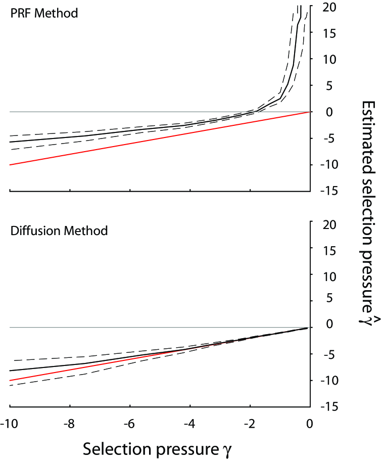
Figure 2: A comparison between the accuracy of inferred selection pressures under the PRF method (top, as in Fig. 1) versus the one-dimensional diffusion method (bottom). In both cases, selection pressures were estimated from the unfolded polymorphism frequencies among $n=14$ sequences sampled from a simulated Wright-Fisher population. Dashed lines indicate 95% confidence intervals around the ML estimates. The line $\hat{\gamma}=\gamma$ is shown in red, and the line $\hat{\gamma}=0$ is shown in gray. Unlike the PRF method, the diffusion method provides unbiased estimates of the selection pressure, and it does not lead to erroneous inferences of positive selection.

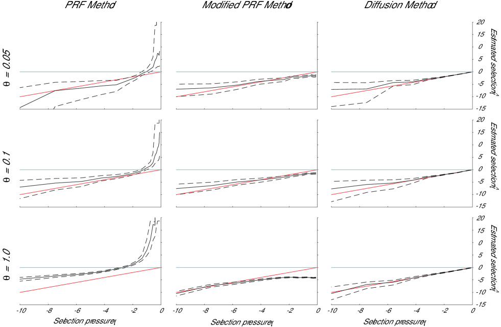
Figure 3: Maximum-likelihood estimates of selection pressures obtained under the PRF method, the modified (per-site) PRF method, and the one-dimensional diffusion method. Selection pressures were estimated from the unfolded polymorphism frequencies among $n=14$ sequences sampled from a simulated Wright-Fisher population. In each panel, the simulated selection pressure $\gamma$ is shown on the $x$-axis, and the estimated selection pressure $\hat{\gamma}$ on the $y$-axis. Dashed lines indicate 95% confidence intervals around the ML estimates. The line $\hat{\gamma}=\gamma$ is shown in red, and the line $\hat{\gamma}=0$ is shown in gray. Simulations and fits were performed across a range of mutation rates, shown in separate rows. The diffusion method and, to a lesser extent, the modified PRF method correct the biases inherent in the original PRF method, especially at large mutation rates.

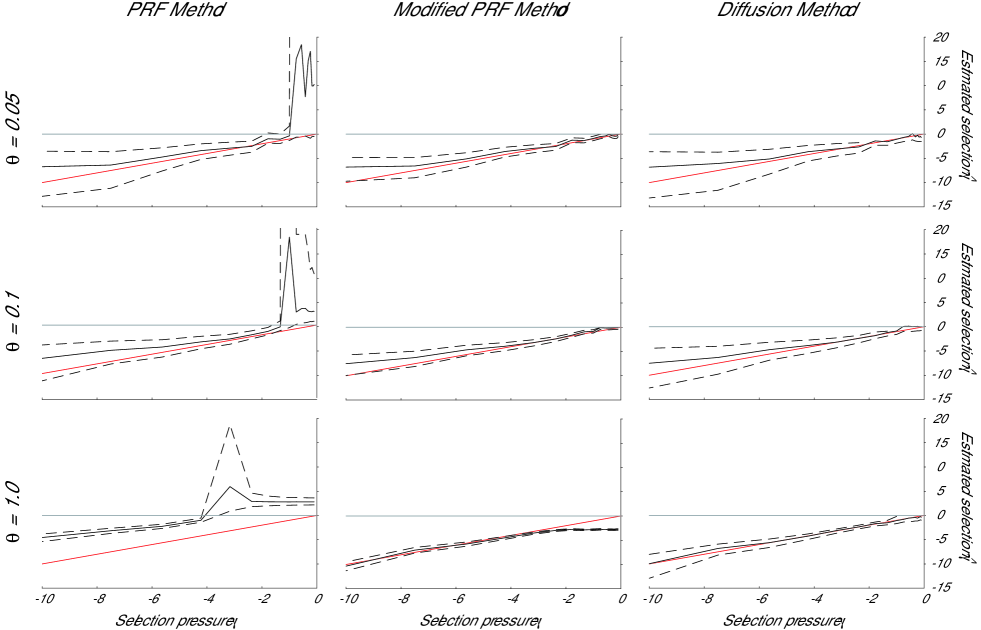
Figure 4: Maximum-likelihood estimates of selection pressures obtained under the PRF method, the modified (per-site) PRF method, and the three-dimensional diffusion method. Selection pressures were estimated from the folded polymorphism frequencies among $n=14$ sequences sampled from a simulated Wright-Fisher population. The diffusion method and, to a lesser extent, the modified PRF method correct the biases inherent in the original PRF method. When selection is weakly negative, the diffusion method cannot reject positive selection on the basis of folded data, as indicated by the lack of the upper confidence interval for some of the fits.

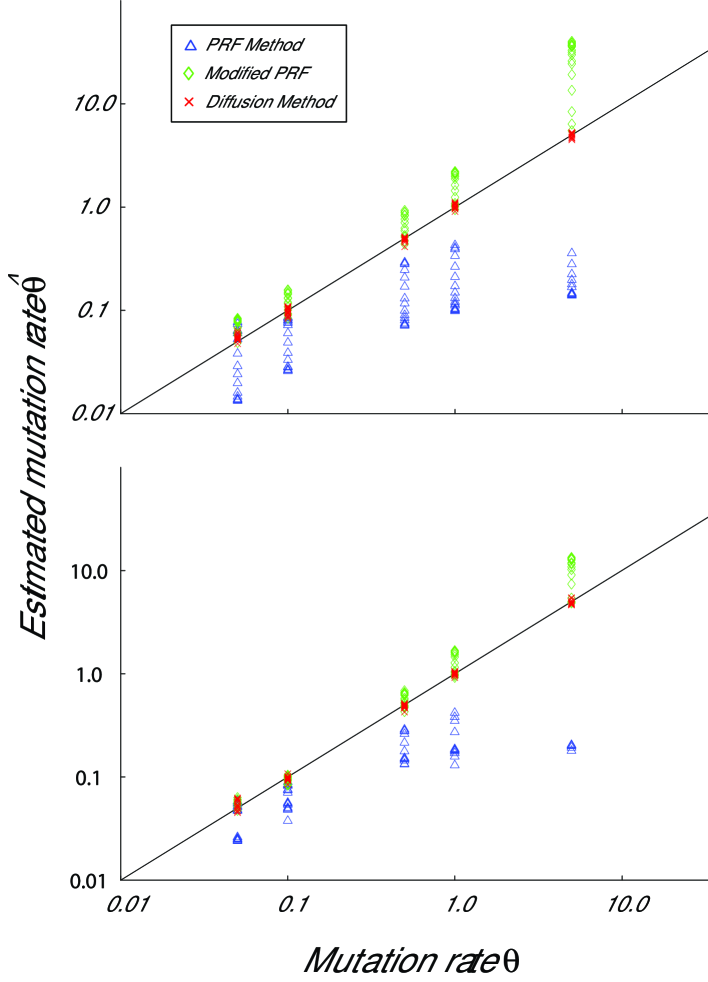
Figure 5: Maximum-likelihood estimates of the mutation rate, $\theta_{s}=2N\mu$, obtained under the PRF method (blue), the modified PRF method (green), and the diffusion methods (red). Mutation rates were estimated from the unfolded (top) and folded (bottom) polymorphism frequencies among $n=14$ sequences sampled from a simulated Wright-Fisher population. The simulated mutation rate $\theta_{s}$ is shown on the $x$-axis, and the estimated mutation rates $\hat{\theta_{s}}$ on the $y$-axis. The line $\hat{\theta_{s}}=\theta_{s}$ is shown in black. For each value of $\theta_{s}$, simulations and fits are shown for 17 different values of $\gamma$, ranging from $\gamma=-10.0$ to $\gamma=-0.1$. The PRF method systematically underestimates the mutation rate, especially when selection is weak. The diffusion methods provide accurate and unbiased estimates of the mutation rate for both folded and unfolded data, across the full range of parameters.

We performed simulations over a wide range of parameter values. We considered five different values of $\theta_{s}$: 0.05, 0.1, 0.5, 1.0, and 5.0. For each value of $\theta_{s}$, we performed one simulation at each of 17 different values of $\gamma$, ranging from $\gamma=-10.0$ to $\gamma=-0.1$. For each set of simulation parameters $(\gamma,\theta_{s})$, once the simulated polymorphism data had been generated, ML parameter estimates $(\hat{\gamma},\hat{\theta_{s}})$ were obtained by numerical maximization of the likelihood function, as specified by the original PRF model, the per-site PRF model, the one-dimensional diffusion model, or the three-dimensional diffusion model. A 95% confidence interval for $\gamma$ was constructed according to Bustamante et al. (2001): the interval includes those values of $\gamma$ within $0.5\chi^{2}_{1,0.95}$ likelihood units from $\hat{\gamma}$. The estimated parameters shown in Figures 1-5 are somewhat ‘jagged,’ because the inference methods have been applied to a single draw of $n=14$ sequences for each set of simulation parameters, as opposed to averaging over many such draws.

As discussed above, the original PRF model disallows multiple mutant lineages at a site. Therefore, when a site sampled from the simulated data exhibited more than two types of segregating nucleotides, the frequencies of all unpreferred nucleotides were summed to represent the frequency of the ‘mutant’ type, as suggested by Hartl et al. (1994). In addition, when fitting folded data using the PRF method, the most common nucleotide was assumed to be the ancestral type, as suggested by Hartl et al. (1994). This approach is not entirely accurate, as discussed above, but it is probably the best option available within the original PRF framework.

Fig. 2 compares the accuracy of estimated selection pressures using the original PRF method versus the the one-dimensional diffusion method. Fig. 3 shows the same type of comparisons over a range of mutation rates, including also the modified, per-site PRF method. The original PRF method systematically underestimates the strength of negative selection, by as much as a factor of 10. In fact, the PRF method strongly rejects the true parameters in over 85% of the cases. In addition, the PRF method often erroneously infers strong positive selection when in fact mutants are under negative selection. These problems are more severe when the mutation rate is large, but also occur for small mutation rates. The smallest mutation rate shown in Fig. 3 is one-half the mutation rate estimated for bacterial genes Hartl et al. (1994). The per-site version of the PRF method that we have developed corrects the most severe problems of the standard PRF method, but it too exhibits systematic biases, especially when selection is weak and the mutation rate large (Fig. 3). The one-dimensional diffusion method that we have developed provides accurate and unbiased estimates of $\gamma$ over the full range of selective pressures and mutation rates (Fig. 3). Like its one-dimensional counterpart, the three-dimensional diffusion method also provides accurate and unbiased estimates over the full range of simulated parameters (not shown).

For folded data, Fig. 4 shows the accuracy of inferred selection pressures using the original PRF method, the per-site PRF method, and the three-dimensional diffusion method. Again, the original PRF method systematically underestimates the strength of selection, and it also erroneously infers positive selection. As before, the per-site PRF method corrects the most severe problems of the original PRF method, but it exhibits systematic biases at large mutation rates (Fig. 4). The three-dimensional diffusion method that we have developed provides unbiased estimates of selection pressures. When selection is weak (i.e. $|\gamma|<1$), however, the confidence intervals on diffusion-based estimates of $\gamma$ are appreciably larger in the folded case, compared to the unfolded case (Fig. 3c versus Fig. 4c). This behavior makes perfect sense: when selection is nearly neutral and the ancestor state is unknown, the frequency distribution does not exhibit sufficient skew to deduce the preferred nucleotide. As a result, the diffusion-based estimator cannot distinguish between weak positive and weak negative selection in the absence of information on the preferred nucleotide (Fig. 4c). Thus, the confidence intervals obtained under the folded diffusion technique properly reflect our inability to estimate the selection pressure precisely when selection is weak.

As shown in Figures 3 and 4, when selection is weakly negative the original PRF method erroneously infers positive selection, regardless of the mutation rate. In fact, this problem occurs in the exact parameter regimes that have been estimated from biological data. For example, on the basis of $n=14$ sampled sequences each $367$-sites long, Hartl et al. (1994) estimated $\gamma=-1.34$ and $\theta_{s}=0.0915$ for silent sites in a bacterial gene. If we simulate $367$ Wright-Fisher sites under these parameters and sample $n=14$ sequences, we find that the most likely parameters fit using the original PRF method are $(\hat{\gamma},\hat{\theta_{s}})=(+18.45,0.067)$. This exercise demonstrates that the PRF method not only infers the wrong sign of selection, but it is also an inconsistent estimator under biologically realistic parameters.

Fig. 5 shows the accuracy of estimated mutation rates using the original PRF method, the per-site PRF method, and the diffusion methods. The original PRF method systematically underestimates the mutation rate, by a factor as large as 30. In the unfolded case, the tendency to underestimate the mutation rate is stronger when selection is weak. Estimates obtained using the per-site PRF method that we have developed partly correct these problems, but still exhibit biases at large mutation rates. Our diffusion-based methods provide accurate and unbiased estimates of the mutation rate, for both folded and unfolded data, across the full range of mutation rates and selection pressures (Fig. 5).

The methods we have developed in this paper also allow us estimate the distribution of selection pressures across sites. In one simple case discussed above, we have presented a procedure for estimating the number of lethal sites and the selective pressure operating on the remaining, non-lethal sites in a gene. This procedure involves estimating $\gamma$ and $\theta$ on the basis of polymorphic sites alone, and thereafter estimating the proportion of observed monomorphic sites that are lethal. In order to assess the power and accuracy of this approach, Table 1 shows the predicted number of monomorphic sites in each of our simulations, compared to the number of monomorphic sites actually observed. Across a large range of selective pressures and mutation rates, this approach typically estimates the number of (non-lethal) monomorphic sites within a few percent. As a result, for a gene of length $L=2000$ sites, one-half of which are lethal, our procedure will accurately predict the number of lethal sites within a few percent; and it will accurately predict the selection pressure on the remaining, non-lethal sites.

The simulations and fits presented in this section reflect our intuitive understanding of the assumptions underlying the PRF model versus the methods we have developed. For example, the PRF method disallows multiple mutant lineages at a site and should therefore lead to systematic underestimates of the mutation rate and selective strength, even when mutations are segregating at low frequency. Our simulations and fits verify this behavior. The per-site PRF method corrects the most problematic aspects of infinite-sites assumption, but it still leads to biased inferences at large mutation rates because it neglects interactions among high-frequency mutant lineages. Finally, the one- and three-dimensional diffusion models avoid the infinite-sites approximation altogether, as reflected by the accuracy of estimates obtained across the full range of parameters.

Discussion

The Poisson Random Field model Sawyer and Hartl (1992) and the associated likelihood procedure for estimating parameters Hartl et al. (1994) are perfectly valid when the assumptions underlying the method are met — namely, infinite sites, free recombination, and constant selective pressure across sites. We have shown, however, that the PRF method leads to severely incorrect inferences in practice, because in reality genes contain a finite number of sites. We have developed three new methods that relax or remove the infinite-sites assumption. These new methods not only fix the problems associated with the PRF method, but they also extend the types of inferences that can be drawn from polymorphism data to include inferences on the distribution of selective pressures across sites.

It may seem surprising that the infinite-sites approximation can lead to such drastic errors in the mutation rates and selective strengths inferred by the PRF method. After all, sites at which multiple mutant lineages are sampled are presumably very rare. Multiple polymorphisms (i.e. three or more segregating nucleotides) occur in only a few percent of sites for much of the data analyzed by the PRF method (e.g. Hartl et al. (1994)). Yet despite their rarity, these sites have a large impact on maximum likelihood estimation of $\gamma$. Because $\gamma$ enters the likelihood function in the factor $e^{2\gamma x}$, changing $\gamma$ has a much larger impact on the likelihood of sites with many mutant nucleotides than those with few. In other words, a single site with a high frequency of mutant nucleotides is very strong evidence for positive selection or low $|\gamma|$, whereas a site with a low frequency of mutant nucleotides is not very strong evidence for the opposite. Thus even a very few sites at which multiple mutant lineages are sampled, but are incorrectly assumed to be the result of a single high-frequency mutant lineage by the original PRF method, can cause large inaccuracies in the inferred $\gamma$. These inaccuracies in $\gamma$ then force corresponding inaccuracies in the inferred $\theta_{s}$.

Previous simulation studies have not observed these problems with the PRF method, and they appear to show that the PRF method makes accurate inferences of mutation rates and selection pressures Bustamante et al. (2001). However, these simulations themselves implicitly assume infinite sites, and hence they cannot be used to test this aspect of the PRF method. In this paper, we have simulated a finite number of sites that evolve according to the Wright-Fisher model that forms the basis of the PRF derivation. As our simulations and fits demonstrate, the infinite-sites assumption causes the original PRF method to systematically underestimate selective pressures and mutation rates, and to find positive selection where it does not in fact exist. The techniques developed here, by contrast, produce accurate estimates of mutation rates and selection pressures across a broad range of biologically reasonable parameters.

The fact that a few highly polymorphic sites have a large impact on the inferred values of $\gamma$ and $\theta_{s}$ points to another important aspect of the original PRF method. In assuming that all sites have the same value of $\gamma$, the PRF method infers some sort of “weighted average” of the variable selection strengths across sites. This is not necessarily a bad thing — in the face of limited data, inferring the full distribution of selection strengths is impossible, and we want instead to have a rough sense of the average strength and direction of selection. However, the exact nature of this “weighting” is unclear. Since a single highly polymorphic site has a much larger effect in reducing the inferred value of $|\gamma|$ (or in suggesting positive selection) than a site with a low frequency of mutant nucleotides has in doing the reverse, the weighting clearly emphasizes neutral, nearly neutral, or positively selected sites more than deleterious sites. In particular, since the PRF method ignores monomorphic sites, it does not weight sites at which mutations are lethal. Thus, the weighting of the original PRF method is useful for increasing the sensitivity of the method to detecting positive selection, but the details of how this weighting works are poorly understood despite being crucial for understanding what an inference of positive selection really means.

The methods we have developed allow us to relax the assumption that all sites have the same $\gamma$, and instead infer aspects of the distribution of selection pressures across sites. It is not yet clear how much data is required to provide adequate power for inferring this distribution to a given resolution. However, we can hope to gain a great deal of insight with only a few additional parameters — say, the number of sites which are neutral, lethal, and negatively selected, and the “weighted average” selection pressure on the latter class. As we have shown, we can estimate the number of lethal sites with no reduction in power relative to the original PRF method, so this proposal would only involve one additional parameter. Additional classes of sites would involve one or two extra parameters each, depending on whether we specify or infer the selection pressure operating on these sites. The appropriate choice of resolution will depend on the context and quality of the data. We hope that experience gained from these approaches will also shed light on the nature of the weighting when a single “average” selection pressure is inferred from the same data, and allow us to interpret this number more precisely.

Unlike the original PRF method, our two diffusion methods do not offer an easy way to infer the existence of positive selection. This limitation arises because positive selection is inherently out of equilibrium. The original PRF method and our modified, per-site PRF method handle this issue by positing rather strange dynamics at individual sites. All mutant lineages are assumed to be positively selected — so if a mutant nucleotide fixes at a given site, mutations back to the ancestral nucleotide are again assumed to be positively selected. While this assumption makes little sense at a per-site level, it allows us to obtain a steady state across sites, provided positive selection is ongoing and not saturated. We could modify our diffusion methods to mimic the PRF treatment of positive selection by changing the boundary conditions in our diffusion equations. Specifically, we would assume that probability flowing into $x=1$ (i.e. fixation of a mutant nucleotide) is absorbed and moved to $x=0$ (i.e. “reset” so that new mutations will again be favored). This diffusion equation can be solved exactly, and the solution used as a basis for inferring positive selection using the the per-site diffusion methods we have developed.

Ideally, however, we would like to infer positive selection in the context of a realistic and well-defined model of the dynamics at individual sites. Such an approach would necessarily involve solutions for the transient dynamics of positively selected mutations sweeping through a population. Kimura (1955) found the full time-dependent solution for the diffusion equation describing the dynamics of a positively selected allele. Such processes are initiated as mutations arise, at Poisson-distributed times. Thus we could construct an expected frequency distribution across sites consisting of a superposition of time-dependent solutions at each site, and use this as the basis for inference of positive selection. In this paper, we do not pursue either of these methods for detecting positive selection within the per-site diffusion framework, but this remains an important direction for future work.

Regardless of the methodology, it will always be difficult to discriminate positive selection from negative selection on the basis of the polymorphism frequency spectrum alone, particularly when only folded data are available. Whether selection is positive or negative, mutant lineages drift nearly neutrally when their frequency is between $0$ and $\frac{1}{|\gamma|}$. Positively selected lineages then fix relatively quickly once their frequency becomes substantially larger than $\frac{1}{|\gamma|}$, while negatively selected lineages rarely ever reach frequencies greater than $\frac{1}{|\gamma|}$. Thus from the point of view of the polymorphism frequency spectrum, positive selection is similar to random drift on $\left[0,1/|\gamma|\right]$, with the upper bound a roughly absorbing boundary condition. Negative selection, on the other hand, is also similar to random drift on $\left[0,1/|\gamma|\right]$, but with the upper bound a roughly reflecting boundary condition. Although this is relatively crude — selection does in fact have some impact on low-frequency lineages, and the boundary conditions are not exactly absorbing or reflecting — it indicates that the polymorphism frequency spectrum is roughly similar for negative and positive selection at the same $|\gamma|$. Thus power to distinguish positive from negative selection based on the polymorphism frequency spectrum, especially with folded data, will always be relatively limited, regardless of the method used.

Inference methods that utilize both interspecies divergence as well as intraspecies polymorphism at synonymous and nonsynonymous sites (i.e. McDonald-Kreitman type tests McDonald and Kreitman (1991)) are often superior to those that rely on the full intraspecific polymorphism frequency spectrum. While these methods lose some power by ignoring information about the full polymorphism frequency spectrum, they utilize data from more than one species as well as a key biological assumption – that synonymous sites are neutral – to provide a sort of internal control. As a result, such methods are typically less sensitive to many of the assumptions of the PRF model Loewe et al. (2006); Sawyer and Hartl (1992), including the infinite-sites assumption. Compared to the original PRF method, violation of the infinite-sites assumption causes less severe errors under McDonald-Kreitman type inferences, because highly polymorphic sites no longer have a disproportionate impact on inferred parameters. The quantification of such biases and the development of a finite-site framework for McDonald-Kreitman type inferences remain topics for future research.

Accuracy of Predicted Number
of Monomorphic Sites
Actual $\theta_{s}$	Average Error	Median Error
$0.05$	$7.6\%$	$7.8\%$
$0.1$	$3.3\%$	$1.8\%$
$0.5$	$2.3\%$	$1.1\%$
$1.0$	$1.4\%$	$0.5\%$
$5.0$	$0.1\%$	$0.1\%$

Table 1: Accuracy of estimates for the expected number of monomorphic sites. We calculated maximum-likelihood estimates of $\gamma$ and $\theta_{s}$ using the one-dimensional diffusion method applied to unfolded simulated data excluding monomorphic sites. From these values, we calculated the expected number of monomorphic sites. Shown are the differences between the observed and expected number of monomorphic sites (in a simulated gene of length $L=1000$ sites). For each value of $\theta_{s}$, we show both the average and median differences in numbers of monomorphic sites, across simulations with $\gamma$ ranging from $-0.1$ to $-10$. These results imply that we can accurately estimate the number of sites monomorphic due to drift. Thus, if a gene contains a similar or larger number of lethal site, we can also estimate the number of such lethal sites to within the above accuracy.

Literature Cited

- Akashi (1995) Akashi, H., 1995 Inferring weak selection from patterns of polymorphism and divergence at ”silent” sites in drosophila dna. Genetics 139: 1067–1076.
- Akashi (1999) Akashi, H., 1999 Inferring the fitness effects of dna mutations from polymorphism and divergence data: Statistical power to detect directional selection under stationarity and free recombination. Genetics 151: 221–238.
- Akashi and Schaeffer (1997) Akashi, H. and S. W. Schaeffer, 1997 Natural selection and the frequency distributions of ”silent” dna polymorphism in drosophila. Genetics 146: 295–307.
- Bartolome et al. (2005) Bartolome, C., X. Maside, S. Yi, A. L. Grant, and B. Charlesworth, 2005 Patterns of selection on synonymous and nonsynonymous variants in drosophila miranda. Genetics 169: 1495–1507.
- Bustamante et al. (2005) Bustamante, C. D., A. Fledel-Alon, S. Williamson, R. Nielsen, M. T. Hubisz, S. Glanowki, D. M. Tanenbaum, T. J. White, J. J. Sninsky, R. D. Hernandez, D. Civello, M. D. Adams, M. Cargill, and A. G. Clark, 2005 Natural selection on protein-coding genes in the human genome. Nature 437: 1153–1157.
- Bustamante et al. (2003) Bustamante, C. D., R. Nielsen, and D. L. Hartl, 2003 Maximum likelihood and bayesian methods for estimating the distribution of selective effects among classes of mutations using dna polymorphism data. Theoretical Population Biology 63: 91–103.
- Bustamante et al. (2002) Bustamante, C. D., R. Nielsen, S. Sawyer, K. M. Olsen, M. D. Purugganan, and D. L. Hartl, 2002 The cost of inbreeding in arabidopsis. Nature 416: 531–534.
- Bustamante et al. (2001) Bustamante, C. D., J. Wakeley, S. Sawyer, and D. L. Hartl, 2001 Directional selection and the site-frequency spectrum. Genetics 159: 1779–1788.
- Ewens (2004) Ewens, W. J., 2004 Mathematical Population Genetics: I. Theoretical Introduction. Springer, New York, NY.
- Galtier et al. (2006) Galtier, N., E. Bazin, and N. Bierne, 2006 Gc-biased segregation of noncoding polymorphisms in drosophila. Genetics 172: 221–228.
- Hartl et al. (1994) Hartl, D. L., E. N. Moriyama, and S. A. Sawyer, 1994 Selection intensity for codon bias. Genetics 138: 227–234.
- Kimura (1955) Kimura, M., 1955 Solution of a process of random genetic drift with a continuous model. PNAS 41: 144–150.
- Lercher et al. (2002) Lercher, M. J., N. G. C. Smith, A. Eyre-Walker, and L. Hurst, 2002 The evolution of isochores: Evidence from snp frequency distributions. Genetics 162: 1805–1810.
- Loewe et al. (2006) Loewe, L., B. Charlesworth, C. Bartolome, and V. Noel, 2006 Estimating selection on nonsynonymous mutations. Genetics 172: 1079–1092.
- McDonald and Kreitman (1991) McDonald, J. and M. Kreitman, 1991 Adaptive protein evolution at the adh locus in drosophila. Nature 351: 652–654.
- Moran (1959) Moran, P. A. P., 1959 The survival of a mutant gene under selection. ii. Journal of the Austrian Mathematical Society 1: 485–491.
- Nachman (1998) Nachman, M. W., 1998 Deleterious mutations in animal mitochondrial dna. Genetica 102/103: 61–69.
- Piganeau and Eyre-Walker (2003) Piganeau, G. and A. Eyre-Walker, 2003 Estimating the distribution of fitness effects from dna sequence data: Implications for the molecular clock. Proceedings of the National Academy of Sciences 100: 10335–10340.
- Rand and Kann (1998) Rand, D. M. and L. M. Kann, 1998 Mutation and selection at silent and replacement sites in the evolution of animal mitochondrial dna. Genetica 102/103: 393–407.
- Sawyer et al. (2003) Sawyer, S., R. J. Kulathinal, C. D. Bustamante, and D. L. Hartl, 2003 Bayesian analysis suggests that most amino acid replacements in drosophila are driven by positive selection. Journal of Molecular Evolution 57: S154–S164.
- Sawyer and Hartl (1992) Sawyer, S. A. and D. L. Hartl, 1992 Population-genetics of polymorphism and divergence. Genetics 132: 1161–1176.
- Wakeley (2003) Wakeley, J., 2003 Polymorphism and divergence for island-model species. Genetics 163: 411–420.
- Watterson (1977) Watterson, G. A., 1977 Heterosis or neutrality? Genetics 85: 789–814.
- Weinreich and Rand (2000) Weinreich, D. M. and D. M. Rand, 2000 Contrasting patterns of nonneutral evolution in proteins encoded in nuclear and mitochondrial genomes. Genetics 156: 385–399.
- Williamson et al. (2004) Williamson, S., A. Fledel-Alon, and C. D. Bustamante, 2004 Population genetics of polymorphism and divergence for diploid selection models with arbitrary dominance. Genetics 168: 468–475.
- Williamson et al. (2005) Williamson, S. H., R. Hernandez, A. Fledel-Alon, L. Zhu, R. Nielsen, and C. D. Bustamante, 2005 Simultaneous inference of selection and population growth from patterns of variation in the human genome. Proceedings of the National Academy of Sciences 102: 7882–7887.
- Wright (1938) Wright, S., 1938 The distribution of gene frequencies under irreversible mutation. Proceedings of the National Academy of Sciences 24: 253–259.
- Wright (1949) Wright, S., 1949 Adaptation and selection. In Genetics, Paleontology, and Evolution, edited by G. L. Jepson, G. G. Simpson, and E. Mayr, pp. 365–389, Princeton University Press, Princeton, NJ.
- Zhu and Bustamante (2005) Zhu, L. and C. D. Bustamante, 2005 A composite-likelihood approach for detecting directional selection from dna sequence data. Genetics 170: 1411–1421.