Semiclassical Propagation of Gaussian Wavepackets

Abstract

We analyze the semiclassical evolution of Gaussian wavepackets in chaotic systems. We prove that after some short time a Gaussian wavepacket becomes a primitive WKB state. From then on, the state can be propagated using the standard TDWKB scheme. Complex trajectories are not necessary to account for the long-time propagation. The Wigner function of the evolving state develops the structure of a classical filament plus quantum oscillations, with phase and amplitude being determined by geometric properties of a classical manifold.

Introduction. The standard approach to semiclassical evolution is time-dependent WKB theory (TDWKB) vanvleck28 ; dirac ; berry79 ; maslov . This theory provides a clear geometric description of the dynamics: a time dependent quantum state is associated with an evolving Lagrangian manifold in classical phase space. [A phase-space manifold $(p(q),q)$ is Lagrangian if $p=\nabla S(q)$, for some generating function $S$ littlejohn92 .] For TDWKB to be applicable the initial state must itself be related to a Lagrangian manifold. This is the case, e.g., of eigenstates of position or momentum operators (related to planes) littlejohn92 , or highly excited eigenstates of bounded integrable Hamiltonians (related to tori) berry79 .

Somewhat surprisingly TDWKB has never been used to propagate Gaussian wavepackets. It is probably the static point of view what blocked the use of standard TDWKB: If a Gaussian state is thought of as the ground state of some harmonic oscillator, then it certainly does not qualify as an initial WKB state. However, by taking the dynamics into consideration, a new perspective arises. In chaotic systems, when one observes the evolution of an initially Gaussian wavepacket through a phase space representation (like Husimi or Wigner) schleich , it becomes manifest that, after some time, the wavepacket acquires the form of a thin filament, very similar to the classical evolution of the initial density tomsovic91 ; zurek03 ; silvestrov03a ; toscano05 (in the case of the Wigner function the filament is decorated by interference fringes). The smaller $\hbar$ (as compared with the relevant action scales), the stronger the localization of the wavepacket along some classical manifold. With this picture in mind it is natural to conjecture that the wavepacket evolves into a WKB state, its support being a real phase-space manifold silvestrov02 ; silvestrov03a ; schubert04 . The purpose of this paper is to prove this statement.

We show that, after some (short) time, a Gaussian wavepacket becomes a primitive WKB state. From then on, the state can be propagated using the standard TDWKB scheme. Complex trajectories maslovII ; huber88 ; aguiar05 are not necessary to describe the long-time propagation of wavepackets, but they may be used to describe the evolution during the initial stage. The present approach not only offers an intuitive geometric description of the evolving state, but can be very accurate, as we demonstrate with a numerical example.

We focus on the Wigner function for its ability to reflect subjacent phase space structures ozorio98 , and because it is the standard representation when dealing with decoherence (arising from coupling to the environment zurek03 ) in semiclassical regimes.

TDWKB approach. In order to eliminate some unnecessary complications in the general problem of semiclassical wavepacket propagation in chaotic systems we consider a one degree of freedom Hamiltonian $H(p,q,t)$, the dependence on $t$ being periodic with period $\tau$. Let us assume that the one-period map, $M_{\tau}(p(t),q(t))=(p(t+\tau),q(t+\tau))$, has a hyperbolic fixed point at the origin, and, without loss of generality, choose the $q$ axis to coincide with the unstable subspace. At $t=0$ we launch a Gaussian wavepacket at the origin:

$$\psi_{0}(q)=(2\pi\sigma^{2})^{-1/4}\exp(-q^{2}/4\sigma^{2})\;.$$ (1)

Note that we have preserved the essential ingredient of chaotic dynamics, i.e., the exponential stretching and folding of phase space manifolds.

If the $q$-uncertainty ($\sigma$) of the initial wavepacket (1) is large enough [e.g., a classical length, $\sigma\sim\hbar^{0}$], then (1) is already a primitive WKB state,

$$\psi_{0}(q)=A_{0}(q)\exp[iS_{0}(q)/\hbar]\;,$$ (2)

given that both the amplitude $A_{0}(q)$ and phase $S_{0}(q)=0$ vary slowly on the quantum scale dirac . The associated Lagrangian manifold is $p=0=dS_{0}/dq$. Accordingly, this state can be successfully evolved using the TDWKB scheme, as we showed in Ref. maia07 .

Let us now analyze what happens when a small circular wavepacket is launched at an unstable fixed point. Numerical simulations show that the positive part of the Wigner function gets stretched along the unstable manifold. As this positive part bends, interference fringes appear. The picture is that of a positive (classical) thin filament decorated by an oscillatory pattern (see Fig. 1).

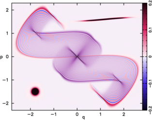
Figure 1: (Color online) Linear density plot of the exact Wigner function [$\pi\hbar\,W(p,q)$] after six periods of evolution with the kicked harmonic oscillator (see the text for a description of the system). We also show displaced versions of (i) the initial state (a circular Gaussian at the origin, left-bottom), (ii) the Wigner function after two steps (top-right).

The fact that the structures in Fig. 1 are very similar to those found in the Wigner functions related to WKB eigenstates berry77 , leads us to enquire: does the Wigner function of Fig. 1 correspond to a WKB state, i.e., can we write

$$\psi_{t}(q)\approx\sum_{\nu}A^{(\nu)}_{t}(q)\exp[\,iS^{(\nu)}_{t}(q)/\hbar]\;?$$ (3)

Here $\nu$ labels the different branches of the hypothetical Lagrangian manifold supporting the WKB state ($p^{(\nu)}=dS^{(\nu)}/dq$) littlejohn92 . It is understood that the expression above must be valid during some time interval, during which amplitudes and phases evolve according to TDWKB theory dirac ; berry79 ; maslov ; littlejohn92 , i.e., amplitudes are convected by the classical flow in $q$-space

$$A_{t}(q^{\prime})=A_{0}(q)\left|\partial q^{\prime}/\partial q\right|^{-1/2}\;,$$ (4)

and the generating function, which solves the Hamilton-Jacobi equation, can be written as an integral over the classically evolved manifold berry79 :

$$S_{t}(q^{\prime})=S_{t}(q_{0})+\int_{q_{0}}^{q^{\prime}}p\,dq\;.$$ (5)

In the case of only one branch, i.e., before the classical manifold folds, a numerical simulation is sufficient to answer the question posed above, as we show in the following. For this purpose we introduce the concrete model system that will serve as our test bench. This is the kicked harmonic oscillator (KHO) berman91 ; zaslavsky ; toscano05 :

$$H(p,q,t)=\frac{p^{2}}{2m}+\frac{1}{2}m\omega^{2}q^{2}+K\cos(kq)\sum_{n=0}^{\infty}\delta(t-n\tau)\,.$$ (6)

The parameters $m=\omega=k=1$, $K=2$ (in appropriate units toscano05 ), and $\tau=\pi/(3\omega)$ guarantee a large chaotic region around the hyperbolic fixed point located at the origin toscano05 . The unstable direction is close to the $q$ axis. We considered an initial circular state ($t=0^{-}$) given by Eq. (1) with $\sigma=0.08$ (corresponding to $\hbar=0.0128$). Some snapshots of its evolution (Wigner functions) are shown in Fig. 1.

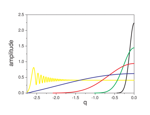
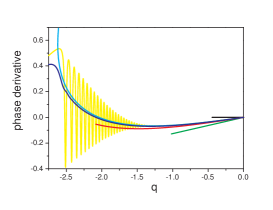
Figure 2: (Color online) Wavefunction amplitude $|\psi_{t}(q)|$ and phase derivative $d\phi_{t}/dq$ (inset) at $t/\tau=0,1,2,3,4$ (black, green, red, blue, yellow, respectively). Also shown is the unstable manifold (inset, cyan). Due to parity symmetry we only plot the region $q\leq 0$.

In Fig. 2 we show amplitude $\rho_{t}(q)$ and phase derivative $d\phi_{t}/dq$ of the evolved state for short times [$\psi\equiv\rho\exp(i\phi/\hbar)$]. Both quantities must be smooth on the quantum scale for the state to qualify as a primitive WKB state. We see that as time grows the amplitude gets smoother: at $t=0$ it was localized in a region of size ${\cal O}(\hbar^{1/2})$, at $t=3$ it has acquired the maximal (classical) width. The derivative of the phase, which is the candidate to Lagrangian support of the WKB state, stays smooth, and close to the unstable manifold, until $t\approx 3$. For larger times, $t\geq 4$, the turning point is reached and a fold is born, giving rise to quantum oscillations in both $\rho(q)$ and $\phi(q)$. For smaller $\hbar$ a similar behavior is observed, the only difference being that it takes longer to reach the turning point (this time goes like $\log\hbar$). Our claim is that, for small enough $\hbar$, there is a time window $(t_{\rm min},t_{\rm max})$ where $\psi_{t}$ is to good accuracy (see below) a primitive WKB state, meaning that it can be propagated further on according to TDWKB. In our numerical example, we checked that the optimal time for starting the TDWKB scheme is $t=2$. At $t=3$ the interference effects of the turning point are already significant (even if not apparent in Fig. 2). At $t=1$ the wavepacket is still not wide enough.

Incidentally, the inset of Fig. 2 shows that TDWKB performs badly if applied at $t=0$. The initial manifold $p=0$ does not evolve classically: it jumps over the unstable direction, instead of staying on the same side.

The next step is thus to evolve $\psi_{t=2}$ using TDWKB and compare with the exact propagation. In order to unfold subjacent phase-space structures, the comparison will be made at the level of Wigner functions.

Semiclassical Wigner function. The Wigner function of a general WKB state [Eq. (3)] can be calculated analytically, using the stationary phase method, in a way analogous to that followed by Berry and Balazs for the special case of semiclassical eigenstates of integrable Hamiltonians berry79 . We start with the usual definition of Wigner function, specialized to our case,

$$W(\bar{p},\bar{q},t)=\frac{1}{\pi\hbar}\int d\xi A_{t}(\bar{q}+\xi)A_{t}(\bar{q}-\xi)e^{i\phi(\xi)/\hbar}\;,$$ (7)

where the phase is given by $\phi(\xi)=S_{t}(\bar{q}+\xi)-S_{t}(\bar{q}-\xi)-2\bar{p}\xi$. We assume that $(\bar{p},\bar{q})$ is not far away from the manifold. In this case only one branch of $S_{t}$ is relevant berry79 . The stationary phase condition reads $p_{t}(\bar{q}+\xi)+p_{t}(\bar{q}-\xi)=2\bar{p}$, where $p_{t}(q)=dS_{t}/dq$. If the point $\bar{x}=(\bar{p},\bar{q})$ is on the concave side of the evolved manifold but not too far away, there are in general two solutions $\pm\xi^{\ast}$, defining two points on the manifold, $x_{+}$ and $x_{-}$. These are the tips of a chord having $\bar{x}$ as midpoint (Fig. 3). When the stationary points are not coalescing they give individual complex conjugate contributions to the integral. The corresponding Wigner function reads

$$W(\bar{p},\bar{q},t)=\frac{2\sqrt{2}}{\sqrt{\pi\hbar}}A_{0}(q_{+})A_{0}(q_{-})\frac{\cos\left({\cal A}/\hbar-\pi/4\right)}{\sqrt{|v_{+}\wedge v_{-}|}}\;.$$ (8)

The phase structure was extracted literally from Ref. berry79 , i.e., ${\cal A}$ is the (symplectic) area between the manifold and the chord. The amplitude is different from Berry and Balazs’, as they considered a different initial density. Here $A_{0}(q_{\pm})$ is the initial amplitude at the preimages of $x_{\pm}$ and $v_{\pm}=dx_{\pm}/dq_{0}\,$ denote tangent vectors at $x_{\pm}$, their moduli representing local rates of expansion ($dq_{0}$ is the $q$ component of a displacement along the initial manifold, at the preimage of $x_{\pm}$).

Equation (8) is a good semiclassical approximation, except in the vicinity caustic points, where $|v_{+}\wedge v_{-}|=0$, i.e., when tangent vectors at the tips of the chords are parallel (see Fig. 3).

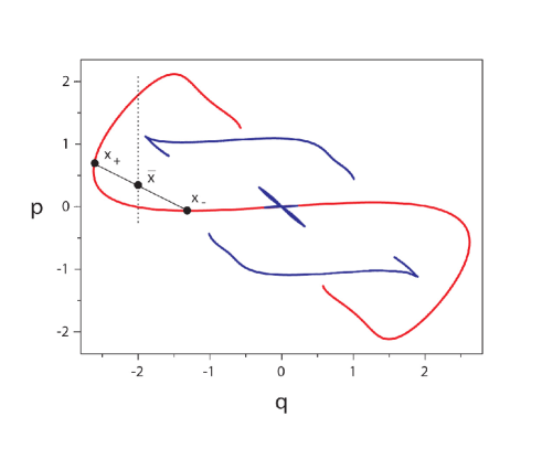
Figure 3: (Color online) Classical manifold corresponding to the state depicted in Fig. 1 (red). This manifold is itself a caustic of the Wigner function. The “ghost” lines (blue) also belong to the caustic. The point $\bar{x}$ is the center of the chord with tips at $x_{-}$ and $x_{+}$. A point $\bar{x}$ belongs to the caustic if the vectors tangent to the manifold at $x_{-}$ and $x_{+}$ are parallel. The dashed vertical line at $q=-2.0$ indicates a special section for testing the semiclassical approximations (see Fig. 4).

At caustics stationary phase points coalesce and one must use transitional (or uniform) approximations berry77 . If $(\bar{p},\bar{q})$ is close enough to the classical manifold, we can obtain a crude transitional approximation to Eq. (7) as follows: (i) Approximate the manifold by the quadratic curve $\bar{p}\approx p_{\ast}+p^{\prime}_{\ast}(q-q_{\ast})+p^{{}^{\prime\prime}}_{\ast}(q-q_{\ast})^{2}/2$. This leads to a cubic phase $\phi(\xi)$. (ii) Neglect variations of the amplitude, i.e., $A_{t}(q)\approx A_{t}(q_{\ast})$. If we traverse the caustic along the line $\bar{q}=q_{\ast}$, and assuming $p^{{}^{\prime\prime}}_{\ast}>0$, then alonso00 ; silvestrov02 :

$$W(\bar{p},q_{\ast},t)\approx\frac{2A_{t}^{2}(q_{\ast})}{(\hbar^{2}p^{{}^{\prime\prime}}_{\ast})^{1/3}}{\rm Ai}\left[-\frac{2(\bar{p}-p_{\ast})}{(\hbar^{2}p^{{}^{\prime\prime}}_{\ast})^{1/3}}\right]\,,$$ (9)

Ai standing for the Airy function.

We are now in position for the final step in our program: the comparison of exact and semiclassical evolutions. Figure 1 displays the exact Wigner function after six steps of evolution. It is evident that its skeleton is the caustic of the manifold of Fig. 3, which was obtained by evolving during four steps the manifold (phase derivative) associated to the exact $\psi_{t=2}(q)$.

For a quantitative examination, in Fig. 4 we plotted the section $q=-2$ of the exact Wigner function together with the semiclassical prediction, Eqs. (8) and (9). Inside their respective domains of validity both approximations are excellent. This completes our argumentation.

Figure 4: A section of the exact Wigner function $W(p,q=-2)$ of Fig. 1 (line) vs. WKB approximation. Full circles correspond to the standard stationary phase result [Eq. (8)] and open circles to the transitional approximation [Eq. (9)].

Concluding remarks. We reported for the first time the use of standard TDWKB for semiclassical propagation of wavepackets in chaotic systems.

The key point is that chaotic dynamics provides the initial expansion that defines the appropriate Lagrangian manifold for starting the TDWKB scheme. In particular we showed that localized states typically evolve into WKB states, and explained how to calculate amplitudes and phases explicitly.

Our results provide a novel perspective for re-examining important previous work on long-time wavepacket propagation. Consider, for instance, the remarkable calculations of Tomsovic and Heller’s, who used a multiple linearization scheme to obtain accurate autocorrelation functions for large times tomsovic91 . In the light of our findings, their scheme can now be understood as arising from the linearization of the WKB wavefunction $\psi_{t}(q)$ (which is globally valid) in the vicinity of a periodic point. The family of “homoclinic” intersections in Ref. tomsovic91 , essential for organizing the summation of recurrences, corresponds, in the TWKB context, to the set of intersections between the Lagrangian manifold of the evolved state and the stable manifold of the fixed point. In this way, we expect the present paper will contribute to the ongoing debate about the timescale for the breakdown of semiclassical propagation. Whether the breaktime diverges like $\log\hbar$ silvestrov02 ; schubert04 or, more plausibly, like some power of $\hbar$ tomsovic91 ; schubert07 is a question still awaiting a definitive answer.

One important feature of TDWKB is that it can be easily supplemented to accommodate decoherence effects. Let us briefly analyse the example of the Lindblad master equation corresponding to a chaotic Hamiltonian system coupled to a high temperature reservoir breuer ; toscano05 (or, similarly, the non-selective weak continuous measurement of $\hat{q}$ and/or $\hat{p}$ breuer ; jacobs06 ). In the formalism of quantum trajectories breuer , the quantum jumps associated to such an environment (or weak measurement scheme), amount to random rigid translations in phase space hall94 . The alternation of random translations with Hamiltonian evolution leads to a final density matrix represented by a weighted ensemble of pure WKB states, each one related to a particular history of random translations. The corresponding Wigner function is thus suggestively expressed as an average over filamentary Wigner functions like the one depicted in Fig. 1.

Acknowledgments. We thank A. M. Ozorio de Almeida, L. A. Pachón, M. Sieber, E. Vergini, T. Dittrich, J. Vanicek, L. Kaplan, G. Alber, and E. J. Heller for interesting comments. Partial financial support from CNPq, CAPES, PROSUL, The Millennium Institute for Quantum Information (Brazilian agencies), and UNESCO/IBSP Project 3-BR-06 is gratefully acknowledged.

References

- (1) J. H. Van Vleck, Proc. Nac. Acad. Sci. 14, 178 (1928).
- (2) P. A. M. Dirac, Principles of Quantum Mechanics (Oxford University Press, Oxford, 1947).
- (3) M. V. Berry and N. L. Balazs, J. Phys. A 12, 625 (1979).
- (4) V. P. Maslov and M. V. Fedoriuk, Semiclassical Approximations in Quantum Mechanics (Reidel, Dordrecht, 1981).
- (5) R. G. Littlejohn, J. Stat. Phys. 68, 7 (1992).
- (6) W. P. Schleich, Quantum Optics in Phase Space (Wiley-VCH, Berlin, 2001).
- (7) S. Tomsovic and E. J. Heller, Phys. Rev. Lett. 67, 664 (1991); Phys. Rev. E. 47, 282 (1993).
- (8) P. G. Silvestrov, J. Tworzydlo, and C. W. J. Beenakker, Phys. Rev E 67, 025204(R) (2003).
- (9) W. H. Zurek, Rev. Mod. Phys. 75, 715 (2003).
- (10) F. Toscano, R. L. de Matos Filho, and L. Davidovich, Phys. Rev. A 71, 010101(R) (2005).
- (11) R. Schubert, Commun. Math. Phys. 256, 239 (2004).
- (12) P. G. Silvestrov and C. W. J. Beenakker, Phys. Rev. E 65, 035208(R) (2002).
- (13) V. P. Maslov, The Complex WKB Method for Nonlinear Equations I (Birkhäuser, Basel, 1994).
- (14) D. Huber, E. J. Heller, and R. G. Littlejohn, J. Chem. Phys. 89, 2003 (1988).
- (15) M. A. M. de Aguiar, M. Baranger, L. Jaubert, F. Parisio, and A. D. Ribeiro, J. Phys. A. 38, 4645 (2005).
- (16) A. M. Ozorio de Almeida, Phys. Rep. 295, 265 (1998).
- (17) R. N. P. Maia, F. Nicacio, R. O. Vallejos, and F. Toscano, arXiv:0707.2423v1 [nlin.CD].
- (18) M. V. Berry, Phil. Trans. Roy. Soc. London Ser. A 287, 237 (1977).
- (19) G. P. Berman, V. Yu. Rubaev, and G. M. Zaslavsky, Nonlinearity 4, 543 (1991).
- (20) G. M. Zaslavsky, R. Z. Sagdeev, D. A. Usikov, and A. A. Chernov, Weak Chaos and Quasi-Regular Patterns (Cambridge University Press, Cambridge, 1992).
- (21) M. A. Alonso and G. W. Forbes, J. Opt. Soc. Am. A 17, 2288 (2000).
- (22) R. Schubert, arXiv:0705.0134v1 [math-ph].
- (23) H.-P. Breuer and F. Petruccione, The Theory of Quantum Open Systems (Oxford University Press, Oxford, 2002).
- (24) K. Jacobs and D. A. Steck, Contemporary Physics 47, 279 (2006).
- (25) M. J. W. Hall, Phys. Rev. A 50, 3295 (1994).