Title:

Noise-Induced Sampling of Alternative Hamiltonian Paths in Quantum Adiabatic Search

Author:

Frank Gaitan
Department of Physics
Southern Illinois University
Carbondale, IL 62901-4401

Pages:

$11$ pages of text (double-space)

Figures:

$5$ figures

Tables:

$4$ tables

Technical Abstract

We numerically simulate the effects of noise-induced sampling of alternative Hamiltonian paths on the ability of quantum adiabatic search (QuAdS) to solve randomly-generated instances of the NP-Complete problem N-bit Exact Cover 3. The noise-averaged median runtime is determined as noise-power and number of bits $N$ are varied, and power-law and exponential fits are made to the data. Noise is seen to slowdown QuAdS, though a downward shift in the scaling exponent is found for $N>12$ over a range of noise-power values. We discuss whether this shift might be connected to arguments in the literature that suggest that altering the Hamiltonian path might benefit QuAdS performance.

Non-Technical Abstract

We numerically simulate the effects of noise on the ability of the Quantum Adiabatic Search (QuAdS) algorithm to solve randomly-generated instances of the NP-Complete problem N-bit Exact Cover 3. The noise-averaged median runtime is determined as noise-power and number of bits N are varied, and power-law and exponential fits are made to the data. Noise is seen to slowdown QuAdS, though a downward shift in the scaling exponent is found for $N>12$ over a range of noise-power values. We discuss whether this shift might be connected to arguments in the literature that suggest that altering the path followed by the search Hamiltonian might benefit QuAdS performance.

Keywords:

quantum adiabatic search; quantum algorithms; computational complexity; NP-Completeness; noise

1 Introduction

One of the deepest open questions in theoretical computer science is whether the computational complexity classes $P$ and $NP$ are equal [1]. It is widely conjectured that these two classes are different, though it is known that should a polynomial-time algorithm be found for an $NP$-Complete problem, then $P=NP$. In 2001, Farhi et. al. [2] examined whether a quantum algorithm might be able to solve an $NP$-Complete problem in polynomial-time. They used the quantum adiabatic search (QuAdS) algorithm [3] to find solutions to randomly-generated hard instances of the NP-Complete problem $N$-bit Exact Cover 3 which they believed to be classically intractable for sufficiently large $N$. Using a digital computer they numerically simulated the QuAdS dynamics. They determined the algorithm’s median runtime to solve this class of instances for a restricted range of $N$ values and found their results could be fit with a quadratic scaling relation. It was noted that should classical algorithms truly require exponential time to solve this class of instances, and should the quadratic scaling behavior of QuAdS persist to large $N$, then QuAdS could outperform classical algorithms on this class of instances, though not necessarily on the worst case instances.

QuAdS works well so long as the quantum dynamics is adiabatic. This requires the runtime $T$ to be large compared to $1/\Delta^{2}$, where $\Delta$ is the smallest value (encountered during the dynamical evolution) of the energy gap between the ground and first-excited states. When $\Delta$ is too small, the adiabatic condition is violated, and QuAdS performance suffers. Farhi and co-workers [4] examined a case where a failure of QuAdS was transformed into a success if the path followed by the search Hamiltonian $H(t)$ differed from the Hamiltonian path used in Refs. [2] and [3] that linearly interpolates from an initial to a final Hamiltonian. The essential point is that, should the linearly interpolating search Hamiltonian produce a $\Delta$ that is too small, varying the Hamiltonian path may cause the new search Hamiltonian to produce a larger $\Delta$ and thus improve QuAdS performance.

A number of papers have considered the robustness of QuAdS performance to noise [5]–[8]. In this paper we extend the simulations reported in Ref. [8] in two important ways. First, the simulation results presented here examine QuAdS performance in the presence of non-uniform noise in which each qubit interacts with a different noise field. Ref. [8] focused on uniform noise. Second, the simulations in this paper are done at larger noise power and larger numbers of qubits $N$. These differences allow the simulations in this paper to sample a larger range of Hamiltonian path variations than was possible in Ref. [8], and so provide a better opportunity to explore how Hamiltonian path variation impacts QuAdS performance.

This paper is organized as follows: (i) Section 2 briefly summarizes the QuAdS algorithm, our noise model, and the simulation protocol; (ii) Section 3 presents our simulation results; and (iii) Section 4 closes with a discussion of these results.

2 Background

We begin with a description of the $NP$-Complete problem $N$-bit Exact Cover 3 (EC3) [1, 2]. An instance of EC3 is specified by a set of clauses $C_{i}$, with $i=1,\ldots,L$, and each clause $C_{i}$ is specified by $3$ integers: $C_{i}=(a(i),b(i),c(i))$. The integers $a(i)$, $b(i)$, and $c(i)$ satisfy $a(i)<b(i)<c(i)$ and take values in the range [$1,\ldots,N$]. Generally, the number of clauses $L$ varies from one EC3 instance to another. A binary vector $z=(z_{1},\ldots,z_{N})$ (with $z_{j}=0,1$) satisfies the clause $C_{i}$ if its components $z_{a(i)}$, $z_{b(i)}$, and $z_{c(i)}$ satisfy $z_{a(i)}+z_{b(i)}+z_{c(i)}=1$. Otherwise, $z$ is said to violate $C_{i}$. A binary vector $z$ solves an instance of EC3 if it satisfies all of its clauses. Finally, an EC3 instance is said to have a unique satisfying assignment (USA instance) if only one binary vector solves it.

In QuAdS an $n$-qubit register is initially prepared in the groundstate of a Hamiltonian $H_{i}$. The only conditions placed on $H_{i}$ are that its groundstate be non-degenerate and easy to prepare. $H_{i}$ is then adiabatically evolved over a time $T$ into a final Hamiltonian $H_{P}$. The final Hamiltonian is constructed so that a basis for its groundstate eigenspace encodes all solutions to the instance of the computational problem that is to be solved. The details of how $H_{P}$ is constructed from an instance of EC3 are described in Ref. [2]. The construction of $H_{i}$ and $H_{P}$ are such that both are dimensionless and have energy-level spacing $\Delta E\sim 1$. Since the initial state is the groundstate of $H_{i}$, the adiabatic dynamics insures that the final state will be in the groundstate eigenspace of $H_{P}$ with probability $P\rightarrow 1$ as $T\rightarrow\infty$. An appropriate measurement of the quantum register at the end of the adiabatic evolution then yields one of the instance solutions. In Refs. [2] and [3] the time-dependent Hamiltonian $H(t)$ that drives the QuAdS dynamics linearly interpolates from $H_{i}$ to $H_{P}$,

$$H(t)=\left(1-\frac{t}{T}\right)H_{i}+\left(\frac{t}{T}\right)H_{P}\hskip 7.22743pt,$$ (1)

where $0\leq t\leq T$, and $T$ is sufficiently large that $H(t)$ produces adiabatic dynamics. The simulations in Ref. [2] randomly generated $75$ USA instances of $N$-bit EC3 which were believed to be hard instances for both classical algorithms and QuAdS. The median runtime $\overline{T}(N)$ for QuAdS to succeed on these instances was found for $7\leq N\leq 20$. It was found that the simulation results could be fit with a quadratic scaling relation $\overline{T}(N)\sim N^{2}$.

To study the impact of noise on QuAdS we introduce classical noise fields $\mathbf{N}_{j}(t)$ ($j=1,\ldots,N$) that couple to the qubits via the Zeeman interaction

$$H_{int}(t)=-\sum_{j=1}^{N}\,\mbox{\boldmath$\sigma$}_{j}\cdot\mathbf{N}_{j}(t)\hskip 7.22743pt.$$ (2)

In this paper we focus on non-uniform noise where each qubit is acted on by a different noise field: $\mathbf{N}_{j}(t)\neq\mathbf{N}_{i}(t)$ ($j\neq i$). A detailed presentation of our noise model is given in Ref. [8]—we summarize its essential properties here. Each noise field $\mathbf{N}_{j}(t)$ is a sequence of randomly occurring fluctuations with profile $\mathbf{F}_{j}(t)$:

$$\mathbf{N}_{j}(t)=\sum_{k=1}^{N_{f}}\,\mathbf{F}_{j}(t-t_{k})\hskip 36.135pt(j=1,\ldots,N)\hskip 7.22743pt.$$ (3)

Here $t_{k}$ is the temporal center of the $k$-th fluctuation and $N_{f}$ is the number of fluctuations. The fluctuations have the following statistical properties: (1) the number of fluctuations $N_{f}$ that occur in a time $T$ is Poisson distributed with average fluctuation rate $\overline{n}$; (2) each fluctuation profile $\mathbf{F}_{j}(t-t_{k})$ is a square pulse with height $x_{j,k}$ and temporal width $2\tau$, where $\tau$ is the thermal relaxation time; (3) the height $x_{j,k}$ is Gaussian distributed with zero mean and variance $\sigma^{2}$; and (4) the times $t_{k}$ are uniformly distributed over [$0,T$]. The simulations allow the polarization of $\mathbf{F}_{j}(t)$ to be either: (i) fixed along $\hat{\mathbf{x}}$, $\hat{\mathbf{y}}$, or $\hat{\mathbf{z}}$; or (ii) to fluctuate simultaneously along all $3$ directions. In Ref. [8] it was found that noise polarized along $\hat{\mathbf{y}}$ caused the largest slowdown of QuAdS and so we focus on $y$-polarized noise throughout this paper. The time-averaged noise power $\overline{P}$ is related [8] to $\overline{n}$, $\sigma^{2}$, and $\tau$ via $\overline{P}=2\overline{n}\sigma^{2}\tau$. The simulations described below use $\sigma=0.2$; $\tau=1$; and average noise power in the range $0.001\leq\overline{P}\leq 0.013$. The average fluctuation rate is then determined from $\overline{n}=\overline{P}/2\sigma^{2}\tau$.

The QuAdS simulation protocol with noise is described in Ref. [8]. As with noiseless QuAdS, the protocol with noise begins by producing $75$ randomly generated USA instances of $N$-bit EC3. The simulations described below were done for $7\leq N\leq 16$. For each USA instance, $10$ noise environments $\{\mathbf{N}_{j}^{m}(t):j=1,\ldots,N;\;m=1,\ldots,10\}$ were generated. For each $m$, $H_{int}(t)$ is determined by plugging the $\{\mathbf{N_{j}}^{m}(t)\}$ into eq. (2). The noiseless QuAdS Hamiltonian $H(t)$ is given by eq. (1), where $H_{i}$ is the same for all USA instances and each USA instance determines its own $H_{P}$ [2]. The noisy QuAdS Hamiltonian $\mathcal{H}(t)$ is then

$$\mathcal{H}(t)=H(t)+H_{int}(t)\hskip 7.22743pt.$$ (4)

For each USA instance and noise environment, $\mathcal{H}(t)$ drives the Schrodinger dynamics of QuAdS. This dynamics is numerically simulated to find the runtime for QuAdS to succeed on that instance and that noise environment. For each $N$, a total of $750=75\times 10$ QuAdS runtimes are generated. The noise-averaged median runtime $\langle\overline{T}(N)\rangle$ is then identified with the median of the $750$ runtimes. We determined the best power-law and exponential fits to the simulation results, and calculate their associated $\chi^{2}_{fit}$ and probability $P(\chi^{2}>\chi^{2}_{fit})$. The simulations were done on the National Science Foundation TeraGrid cluster.

3 Results

We now present our simulation results. As a baseline for the noisy simulations we repeat the noiseless calculation of Ref. [2] for $7\leq N\leq 19$. Our results appear in Figure 1 which contains best power-law and exponential fits to the data. The power-law fit $\overline{T}(N)=aN^{b}$ has fit parameters $a=0.1016$ and $b=2.079$. The value of $\chi^{2}$ for the fit is $\chi^{2}_{fit}=0.321$ and the probability $P(\chi^{2}>\chi^{2}_{fit})=0.9999$. The closer this probability is to $1$, the more consistent the data-set is with the fitting function. The exponential fit $\overline{T}(N)=a[\exp(bN)-1]$ has: (i) fit parameters $a=4.707$ and $b=0.1282$; (ii) $\chi^{2}_{fit}=0.296$; and (iii) probability $P(\chi^{2}>\chi^{2}_{fit})=0.9999$. Both fits are excellent and the power-law fit is consistent with the result of Ref. [2].

The results for our noisy QuAdS simulations appear in $3$ figures and $2$ tables. Figures 2, 3 and 4 plot the noise-averaged median runtime $\langle\overline{T}(N)\rangle$ versus $N$ for average noise power $\overline{P}=(0.001,0.003)$; $(0.005,0.007)$; and $(0.009,0.013)$, respectively. As in Figure 1, each plot contains a power-law ($\langle\overline{T}(N)\rangle=aN^{b}$) and exponential ($\langle\overline{T}(N)\rangle=a[\exp(bN)-1]$) fit to the simulation results. The parameters associated with the power-law and exponential fits appear, respectively, in Tables 1 and 2. For each value of $\overline{P}$ simulated, each Table contains: (i) the best fit parameters $a$ and $b$; (ii) the chi-squared for the fit $\chi^{2}_{fit}$; and (iii) the probability $P(\chi^{2}>\chi^{2}_{fit})$. As noted above, the closer the latter probability is to $1$, the more consistent the data-set is with the fitting function. A discussion of these results is given in the following Section.

4 Discussion

Ref. [4] examined the consequences of modifying the original linearly interpolating QuAdS Hamiltonian $H(t)$ in eq. (1) to

$$\mathcal{H}(t)=H(t)+\delta\mathcal{H}(t)\hskip 7.22743pt,$$ (5)

where the new term $\delta\mathcal{H}(t)$ has the form

$$\delta\mathcal{H}(t)=e(t)\,H_{E}\hskip 7.22743pt,$$ (6)

and the envelope function $e(t)$ is required to vanish at $t=0$ and $T$. Ref. [4] gave $3$ proposals for $H_{E}$, though it will not be necessary to review them here as we have a specific form in mind for $\delta\mathcal{H}(t)$ (see below). Eq. (5) specifies a path in the space of $2^{N}\times 2^{N}$ Hermitian matrices that begins and ends at $H_{i}$ and $H_{P}$, respectively, and which by construction, differs from the linearly interpolating path specified by $H(t)$. As noted in Section 1, Ref. [4] showed that by doing such a path variation, a failure of QuAdS could be converted into a success.

Including a noise interaction in the QuAdS Hamiltonian also causes the Hamiltonian path to deviate from the linearly interpolating path traced out by $H(t)$. For non-uniform $y$-polarized noise, the noise term in eq. (2) is

$$\delta\mathcal{H}(t)=-\sum_{j=1}^{N}\,N_{j}(t)\sigma_{y}^{j}\hskip 7.22743pt,$$ (7)

where $\sigma_{y}^{j}$ is the Pauli matrix $\sigma_{y}$ for qubit $j$ and $N_{j}(t)\,\hat{\mathbf{y}}$ is the noise field that interacts with this qubit. Unlike the envelope function $e(t)$, the noise fields $\{N_{j}(t):j=1,\ldots,N\}$ need not vanish at $t=0$ or $T$. We now show, however, that for the noise used in the simulations presented here and in Ref. [8], the probability that a fluctuation is present at these times is small. To see this, note that for a fluctuation $i$ to be present at $t=0$ ($T$), the fluctuation center $t_{i}$ must occur within a time $\tau$ of $t=0$ ($T$) since the temporal width of the fluctuation is $2\tau$. For our noise model, the time $t_{i}$ has a uniform probability distribution over the time interval [$0,T$] so the probability that $t_{i}$ is within $\tau$ of $t=0$ ($T$) is $\tau/T$. Since $\overline{n}$ is the average fluctuation rate, the average number of fluctuations $\overline{N}_{\tau}$ that occur in a time interval $\tau$ is $\overline{N}_{\tau}=\overline{n}\,\tau$. Since $\overline{n}=\overline{P}/2\sigma^{2}\tau$ (see Section 2), the total probability that a fluctuation is present at $t=0$ ($T$) is

$$P_{tot}=\frac{\overline{P}\,\tau}{2\sigma^{2}T}\hskip 7.22743pt.$$ (8)

For $\overline{P}=0.001$ ($0.013$), the midpoint for the range of $\langle\overline{T}(N)\rangle$ values found in the simulation is approximately $20$ ($39$). Using this value for $T$ in eq. (8), and recalling that our simulations used $\sigma=0.2$ and $\tau=1$ gives $P_{tot}=6.25\times 10^{-4}$ ($4.17\times 10^{-3}$) for $\overline{P}=0.001$ ($0.013$). Thus, with high probability, our noise interaction vanishes at $t=0$ ($T$), and our $\mathcal{H}(t)$ is equal to $H_{i}$ ($H_{P}$) at this time.

For non-uniform $y$-polarized noise, $\delta\mathcal{H}(t)$ has $N$ noise fields $N_{j}(t)$, where $7\leq N\leq 16$ in our simulations. By comparison, the simulations in Ref. [8] used uniform noise in which all qubits see the same noise field $N_{j}(t)=N(t)$, with $j=1,\ldots,N$. Thus our noise interaction with non-uniform $y$-polarized noise has an order of magnitude more variation parameters than the uniform noise used in Ref. [8]. Furthermore, since the non-uniform noise simulations were done to larger values of $\overline{P}$ than the simulations with uniform noise, each noise field in the former case has a larger average number of fluctuations $\overline{N}_{f}$ than in the latter case since $\overline{N}_{f}=\overline{P}T/2\sigma^{2}\tau$. Thus, because the simulations in the present paper were done using: (i) non-uniform noise; (ii) larger average noise power; and (iii) larger number of qubits, they contain larger Hamiltonian path variations than was possible in Ref. [8].

The simulation results presented in Tables 1 and 2 show that the scaling exponent $b$ begins to decrease for $\overline{P}\geq 0.005$. (As will be discussed below, we anticipate that there will be a maximum $\overline{P}$ value beyond which noise will begin to compromise QuAdS perfromance.) A second observation is that power-law scaling provides an excellent fit for all values of $\overline{P}$ simulated, while the exponential fit is not quite as good for $\overline{P}\geq 0.007$. To compare our results with those in Ref. [8] a restricted power-law fit to the non-uniform noise results was done for $7\leq N\leq 12$ and $\overline{P}=(0.001,0.003,0.005)$. This corresponds to the range of $N$ and $\overline{P}$ values simulated in Ref. [8] for uniform $y$-polarized noise. The parameters for the restricted fit, together with the corresponding fit parameters for uniform $y$-polarized noise appear in Table 3. Note that a similar comparison is possible with exponential fits, though nothing new is learned and so we do not include that comparison here. From Table 3 we see that the scaling exponent is comparable for the two types of noise, with smaller $b$-values for non-uniform noise. Compared to the $\overline{P}=0.000$ results, we see that noise slows down QuAdS, but Table 3 gives a first indication that non-uniform noise may allow conditions for the slowdown to be ameliorated.

A look at Figures 3 and 4 shows that the initial rate of growth of $\langle\overline{T}(N)\rangle$ appears to flatten out at intermediate values of $N$. This flattening out is less pronounced for $\overline{P}=0.005$, occurring over the range $12\leq N\leq 14$; and is broader for $\overline{P}=0.013$, occurring over the range $10-11\leq N\leq 14$. To test this observation we did separate fits for each of the data-sets in these Figures at small $N$ ($7\leq N\leq 10$) and (relatively) large $N$ ($13\leq N\leq 16$). The parameters for the two fits appear in Table 4. As above, we only show results for a power-law fit. Table 4 indicates that the small $N$ fit grows at a faster rate (viz. larger $b$) than the large $N$ fit. We see that the flattening out of $\langle\overline{T}(N)\rangle$ at intermediate $N$ marks a crossover from rapid initial growth to a region of slower growth. In an effort to further highlight this point, Figure 5 replots the data for $\overline{P}=0.009$, including the fits for small and large $N$. One clearly sees the data initially following the faster rising fit ($b=3.560$) and then crossing over to the slower rising fit ($b=2.774$). Although noise is plainly causing QuAdS to slowdown relative to noiseless QuAdS (see Figure 1), Table 4 indicates that non-uniform $y$-polarized noise can, for appropriate values of $\overline{P}$ and $N$, ameliorate the slowdown. One might wonder whether there is a connection between this ameliorating effect and the suggestion made in Ref. [4] that varying the Hamiltonian path away from the linearly interpolating path used in Refs. [2] and [3] might improve QuAdS performance. From that perspective, one might wonder whether, for $12<N\leq 16$, non-uniform $y$-polarized noise with $0.005\leq\overline{P}\leq 0.013$ is inducing sufficient variation of the linearly interpolating Hamiltonian path to yield alternative paths with slightly larger minimum energy gaps, causing a (slightly) improved adiabaticity, and so reducing (slightly) the noise-induced slowdown of QuAdS seen at smaller $N$ values. A proper examination of this ansatz requires that the minimum gaps be determined for the USA instances and noise realizations that we simulated in this paper. We plan to carry out this analysis in future work. Note that for sufficiently large average noise power, noise-induced decoherence should ultimately rob QuAdS of its quantum performance-enhancements since it will cause the dynamics to crossover from quantum to classical. A quantitative determination of how this loss of quantum performance occurs presents a significant (though fascinating) challenge for future simulations.

Figure Captions

Figure 1:

Noiseless QuAdS simulation results for the median runtime $\overline{T}(N)$ (dimensionless units) versus number of bits $N$. The solid line is the best power-law fit to the data and the dash-dot line is the best exponential fit. The error bars give $95\%$ confidence limits on the median.

Figure 2:

Simulation results for the noise-averaged median runtime $\langle\overline{T}(N)\rangle$ (dimensionless units) versus number of bits $N$. The noise is polarized along $\hat{\mathbf{y}}$ and has average noise power $0.001$ and $0.003$ (dimensionless units). Each datapoint is the median of $750$ runtimes ($75$ USA instances and $10$ noise environments per USA instance). The solid-line is the best power-law fit to the data and the dash-dot line is the best exponential fit. The error bars give $95\%$ confidence limits for each median.

Figure 3:

Simulation results for the noise-averaged median runtime $\langle\overline{T}(N)\rangle$ (dimensionless units) versus number of bits $N$. The noise is polarized along $\hat{\mathbf{y}}$ and has average noise power $0.005$ and $0.007$ (dimensionless units). Each datapoint is the median of $750$ runtimes ($75$ USA instances and $10$ noise environments per USA instance). The solid-line is the best power-law fit to the data and the dash-dot line is the best exponential fit. The error bars give $95\%$ confidence limits for each median.

Figure 4:

Simluation results for the noise-averaged median runtime $\langle\overline{T}(N)\rangle$ (dimensionless units) versus number of bits $N$. The noise is polarized along $\hat{\mathbf{y}}$ and has average noise power $0.009$ and $0.013$ (dimensionless units). Each datapoint is the median of $750$ runtimes ($75$ USA instances and $10$ noise environments per USA instance). The solid-line is the best power-law fit to the data and the dash-dot line is the best exponential fit. The error bars give $95\%$ confidence limits for each median.

Figure 5:

Re-plot of the simulation results for $\overline{P}=0.009$. The dashed (solid) curve is a restricted power-law fit $\langle\overline{T}(N)\rangle=aN^{b}$ through the data $7\leq N\leq 10$ ($13\leq N\leq 16$). Similar plots are possible for the other $\overline{P}$–values in Table 4, though we do not include them to avoid repetition.

Table 1: Best fit parameters for power-law scaling $\langle\overline{T}(N)\rangle=aN^{b}$ for all values of average noise power $\overline{P}$ simulated. For comparison, best-fit parameters for noiseless QuAdS are also included.

$\overline{P}$	$a$	$b$	$\chi^{2}_{fit}$	$P(\chi^{2}>\chi^{2}_{fit})$
$0.000$	$0.1016$	$2.079$	$0.321$	$0.9999$
$0.001$	$0.07863$	$2.200$	$0.539$	$0.9993$
$0.003$	$0.02595$	$2.753$	$0.869$	$0.9967$
$0.005$	$0.02611$	$2.816$	$1.097$	$0.9976$
$0.007$	$0.03783$	$2.698$	$2.919$	$0.9393$
$0.009$	$0.07251$	$2.458$	$3.449$	$0.9032$
$0.013$	$0.1636$	$2.148$	$2.689$	$0.9523$

Table 2: Best fit parameters for exponential scaling $\langle\overline{T}(N)\rangle=a[\exp(bN)-1]$ for all values of average noise power $\overline{P}$ simulated. For comparison, best-fit parameters for noiseless QuAdS are also included.

$\overline{P}$	$a$	$b$	$\chi^{2}_{fit}$	$P(\chi^{2}>\chi^{2}_{fit})$
$0.000$	$4.707$	$0.1282$	$0.296$	$0.9999$
$0.001$	$2.208$	$0.1845$	$0.185$	$0.9999$
$0.003$	$1.580$	$0.2302$	$0.517$	$0.9994$
$0.005$	$3.123$	$0.1915$	$3.307$	$0.9136$
$0.007$	$3.924$	$0.1799$	$4.833$	$0.7753$
$0.009$	$5.445$	$0.1601$	$4.927$	$0.7653$
$0.013$	$7.112$	$0.1440$	$3.172$	$0.9231$

Table 3: Comparison of power-law fit $\langle\overline{T}(N)\rangle=aN^{b}$ for non-uniform and uniform (Ref. [8]) $y$-polarized noise for $7\leq N\leq 12$ and average noise power $\overline{P}=0.001$, $0.003$, and $0.005$.

$\overline{P}$	non-uniform		uniform
$-$	$a$	$b$	$a$	$b$
$0.001$	$1.107\times 10^{-1}$	$2.044$	$9.677\times 10^{-2}$	$2.108$
$0.003$	$5.095\times 10^{-2}$	$2.439$	$2.982\times 10^{-2}$	$2.679$
$0.005$	$1.677\times 10^{-2}$	$3.020$	$6.607\times 10^{-3}$	$3.429$

Table 4: Restricted power-law fits $\langle\overline{T}(N)\rangle=aN^{b}$ for the $\overline{P}=0.005,0.007,0.009,0.013$ data-sets for: (i) $7\leq N\leq 10$; and (ii) $13\leq N\leq 16$.

$\overline{P}$	$7\leq N\leq 10$		$13\leq N\leq 16$
$-$	$a$	$b$	$a$	$b$
$0.005$	$3.064\times 10^{-2}$	$2.730$	$6.554\times 10^{-2}$	$2.465$
$0.007$	$7.637\times 10^{-3}$	$3.450$	$2.984\times 10^{-2}$	$2.767$
$0.009$	$7.086\times 10^{-3}$	$3.560$	$2.934\times 10^{-2}$	$2.774$
$0.013$	$3.201\times 10^{-2}$	$2.924$	$3.060\times 10^{-2}$	$2.759$

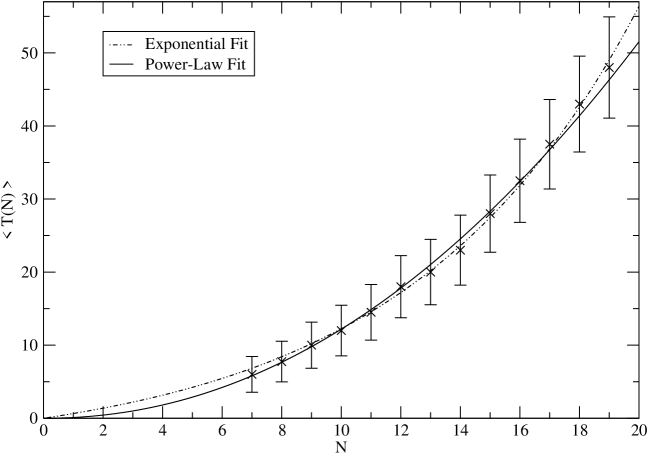
Figure 1:

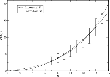
(a) $\overline{P}=0.001$

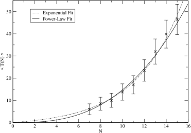
(b) $\overline{P}=0.003$

Figure 2:

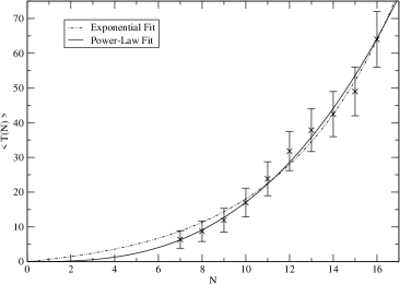
(a) $\overline{P}=0.005$

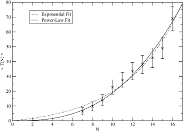
(b) $\overline{P}=0.007$

Figure 3:

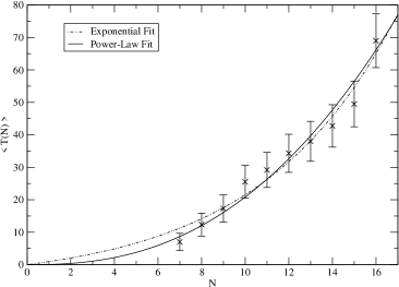
(a) $\overline{P}=0.009$

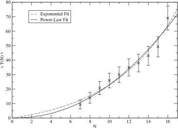
(b) $\overline{P}=0.013$

Figure 4:

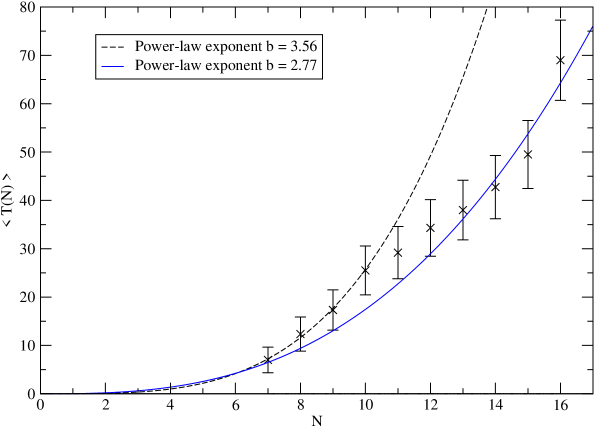
Figure 5:

References

- [1] M. R. Garey and D. S. Johnson, Computers and Intractability, W. H. Freeman and Company, New York, 1979.
- [2] E. Farhi et. al., A quantum adiabatic evolution algorithm applied to random instances of an NP-Complete problem, Science 292, 472, 2001.
- [3] E. Farhi et. al., Quantum computation by adiabatic evolution, http://arXiv.org/abs/quant-ph/0001106.
- [4] E. Farhi, J. Goldstone, and S. Gutmann, Quantum adiabatic evolution algorithms with different paths, http://arXiv.org/abs/quant-ph/0208135.
- [5] A. M. Childs and E. Farhi, Robustness of adiabatic quantum computation, Phys. Rev. A 65, 012322, 2001.
- [6] J. Roland and N. J. Cerf, Noise resistance of adiabatic quantum computation using random matrix theory, Phys. Rev. A 71, 032330, 2005.
- [7] S. Ashhab, J. R. Johansson, and F. Nori, Decoherence in a scalable adiabatic quantum computer, Phys. Rev. A 74, 052330, 2006.
- [8] F. Gaitan, Simulation of quantum adiabatic search in the presence of noise, Int. J. Quantum Info. 4, 843, 2006.