Photometric Redshifts and Signal-to-Noise

Abstract

We investigate the impact of photometric signal-to-noise (S/N) on the precision of photometric redshifts in multi-band imaging surveys, using both simulations and real data. We simulate the optical 4-band (BVRz) Deep Lens Survey (DLS, Wittman et al. 2002), and use the publicly available Bayesian Photometric Redshift code BPZ  by Benitez (2000). The simulations include a realistic range of magnitudes and colors and vary from infinite S/N to $S/N=5$. The real data are from DLS photometry and two spectroscopic surveys, and explore a range of S/N by adding noise to initially very high S/N photometry. Precision degrades steadily as S/N drops, both because of direct S/N effects and because lower S/N is linked to fainter galaxies with a weaker magnitude prior. If a simple S/N cut were used, $S/N\geq 17$ in R (corresponding, in the DLS, to lower S/N in other bands) would be required to keep the scatter in ${\Delta z}\equiv{{z_{\rm spec}}-{z_{\rm phot}}\over 1+{z_{\rm spec}}}$ to less than 0.1. However, cutting on ODDS (a measure of the peakiness of the probability density function provided by BPZ) greater than 0.4 provides roughly double the number of usable galaxies with the same $\sigma_{{\Delta z}}$. Ellipticals form the tightest ${z_{\rm spec}}-{z_{\rm phot}}$ relation, and cutting on type=elliptical provides better precision than the $ODDS>0.9$ cut, but this eliminates the vast majority of galaxies in a deep survey. In addition to being more efficient than a type cut, ODDS also has the advantages of working with all types of galaxies (although ellipticals are overrepresented) and of being a continuous parameter for which the severity of the cut can be adjusted as desired.

1 Introduction

Photometric redshifts (Connolly et al.  1995, Hogg et al.  1998, Benitez 2000) are of paramount importance for current and planned multi-band imaging surveys. With photometric redshifts, surveys can inexpensively gather information about structure along the line of sight, without resorting to expensive spectroscopic followup. Therefore, it is important to understand systematic errors and limitations in this method. For example, Ma et al.  2006 and Huterer et al.  2006 have examined the required photometric redshift accuracy for surveys which plan to use weak lensing (cosmic shear) to constrain dark energy. For this application and also for baryon acoustic oscillations (Zhan & Knox 2006), reducing photometric redshift errors is less important than knowing the error distribution accurately. Thus, careful attention must be paid to systematic differences between the photometric survey and the spectroscopic sample used to evaluate photometric redshift performance. For most surveys, photometric S/N is one of the systematic differences.

The most well-known test case for photometric redshifts is the blind test in the Hubble Deep Field North (HDFN) conducted by Hogg et al.  (1998). The best methods then yielded $\sigma_{{\Delta z}}\sim 0.1$, where ${\Delta z}\equiv{{z_{\rm spec}}-{z_{\rm phot}}\over 1+{z_{\rm spec}}}$, using Hubble Space Telescope (HST) photometry in UBVI bands and ground JHK (Dickinson  1998). More recently, with improved photometry and spectral redshift classification, an accuracy of $\sigma{\Delta z}\sim 0.06$ is achieved over the redshift range 0—6 (Fernandez-Soto et al.  1999, 2001; Benitez 2000). Ground-based surveys suffer from less precise photometry but usually do not have to deal with such a large redshift range. Ilbert et al.  2007 cite an accuracy of $\sigma_{{\Delta z}}=0.029$ after clipping outliers with ${\Delta z}>0.15$ (3.8% of the sample). Ilbert et al.  2007 also find a decrease in precision at fainter magnitudes, but made no effort to separate the effects of S/N from the other effects operating on faint galaxies, such as a weaker magnitude prior and greater SED evolution. In this paper, we examine the impact of these effects separately, focusing on photometric S/N. The quantitative results presented here are specific to the BVRz filter set used in the Deep Lens Survey (DLS, Wittman et al.  2002). More filters, covering a wider range in wavelengths, will do better (Abdalla et al.  2007). However, the trends with S/N are broadly applicable.

2 Method

We use the BPZ  Bayesian photometric redshift code developed by Benitez (2000). We also tested the HyperZ code (Bolzonella et al.  2000) with additional priors roughly equivalent to the default BPZ priors, and found similar performance. For clarity we present only results from BPZ here. We did not test training-set methods, in which a spectroscopic and photometric training set is used to perform a fit or to train a neural network, for two reasons. First, training set methods are unlikely to be employed for surveys planning to push the photometric sample deeper than the spectroscopic sample. Second, the two methods seem to be roughly equivalent in performance on the data sets in which they have been compared (e.g. Hogg et al.  1998), so the trends presented here should be applicable to both methods.

We use the six spectral energy distribution (SED) templates from Benitez (2000): E, Sbc, Scd, Irr, SB3, and SB2, modified as described below. For the simulations, the same templates are used to simulate the photometry and to infer the photometric redshifts; there is no allowance for cosmic variance of the templates or “template noise”. For the data, it is important that the templates reflect real SEDs. Therefore, we use the photometry of objects with spectroscopic redshifts to optimize the templates (Csabai et al.  2000; Benitez et al.  2004; Ilbert et al.  2007). Section 4.2 describes the procedure and shows the corrected templates. Clearly, even the optimized templates do not represent all types of SEDs in the universe. For both simulations and data, we start by demonstrating the performance with as nearly perfect a data set as possible. After illustrating the best-case scenarios, we proceed to degrade the simulations and data to successively lower S/N, repeating the analysis for each step.

For each galaxy, we identify the peak of its redshift probability density function (PDF) as its photometric redshift or $z_{\rm phot}$. This greatly simplifies the analysis and presentation of the results, at the cost of some precision. Specifically, “catastrophic outliers” will appear, whose $z_{\rm phot}$ differs greatly from their true redshift. In many cases, this may be an artifact of not considering the full PDF, a point argued forcefully in the case of the HDF by Fernandez-Soto et al. (2001, 2002). The full PDF may contain additional peaks, or otherwise be broad enough to be consistent with the true redshift. In this paper, we wish to focus on the trends with photometric S/N rather than the characterization of outliers. As will be seen in the tables and figures, the trends with S/N are not substantively changed if “outliers” are removed. Therefore we judge this simplification to be acceptable. “Outlier” in this paper thus refers to difference between $z_{\rm phot}$ and true redshift, without implying anything about the full PDF.

We do consider characteristics of the PDF when using BPZ’s ODDS parameter. BPZ assumes a natural error (template noise) of $0.067(1+z)$, and defines ODDS as the fraction of the area enclosed by the PDF between $zphot\pm n\times 0.067(1+z)$, where $n$ is a user-settable parameter which we set to 1. ODDS values close to unity indicate that most of the area under the redshift probability density function (PDF) is within $Z_{B}\pm 0.067(1+z)$. In this paper, we present results both for the entirety of a given sample, and after a cut of $ODDS>0.9$, which eliminates many of the “outliers.” We also investigate the tradeoff between ODDS cut, number of usable galaxies, and photometric redshift accuracy.

The error distributions are typically non-Gaussian, often highly so. The rms or standard deviation is extremely sensitive to even a few non-Gaussian events, so in the photometric redshift literature, results are usually quoted as an rms after excluding a certain (small) fraction of galaxies as “catastrophic outliers.” The fraction varies from paper to paper, making comparison difficult. The field of robust statistics suggests several less sensitive metrics of variation, such as the median or mean absolute deviation. However, outliers should be included in the performance analysis with some weight, because they will be included when using the entire photometric sample for science. We therefore clip conservatively, $|{\Delta z}|<0.5$, to avoid overly optimistic results. This threshold is at least five, and usually many more, times the clipped rms. We also present, in many cases, differential and cumulative distributions as well. To make the connection with forecasts for, say, weak lensing tomography, we suggest these distributions be fit with double Gaussians. Gaussians are analytically tractable, and a double Gaussian can fit both the core and wings (but not truly catastrophic outliers).

3 Simulations

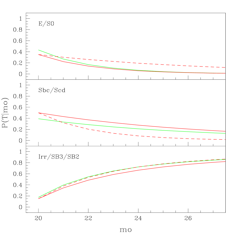
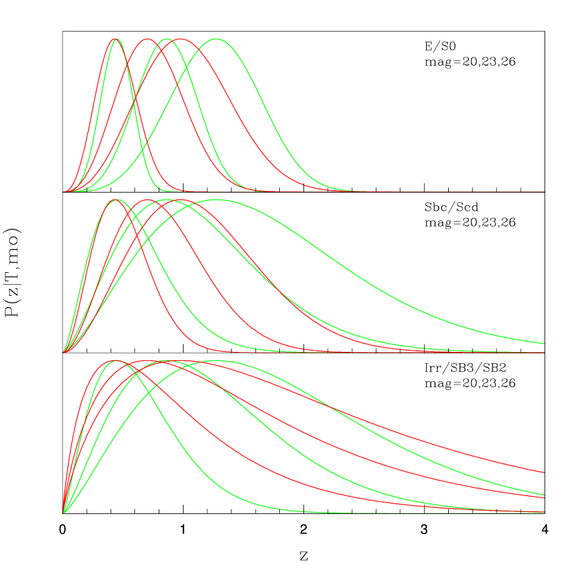
Figure 1: Priors used to populate the simulations. Left: $P(T|m_{0})$ is the galaxy type fraction as a function of magnitude; Right: $P(z|T,m_{0})$ is the redshift distribution for galaxies of a given spectral type and magnitude for $mag=20,23,26$. Throughout this paper we use the priors indicated by the solid red lines (BPZ code). The dashed red lines represent the priors in BPZ’s paper (Benitez 2000), while the green lines indicate the priors derived by Ilbert et al. (2007).

We simulate a mix of ellipticals, spirals, irregulars and starburst galaxies (specifically, E, Sbc, Scd, Irr, SB3, and SB2 templates) following the priors for galaxy type fraction as a function of magnitude, $P(T|m_{0})$, and for the redshift distribution for galaxies of a given spectral type and magnitude, $P(z|T,m_{0})$, that are used in BPZ’s Bayesian photometric redshift code. We found that in Table 1 of Benitez (2000), two numbers were inadvertently switched, but the numbers were correct in the publicly downloadable code. Benitez (private communication) has confirmed that the table should read $k_{t}=0.450$ for E/SO and $k_{t}=0.147$ for Sbc/Scd. Figure 1 shows in solid red lines the priors used in this paper (same as BPZ’s code); in dashed red lines are the priors quoted in BPZ’s paper; and green lines represent Ilbert et al.  (2007) priors.

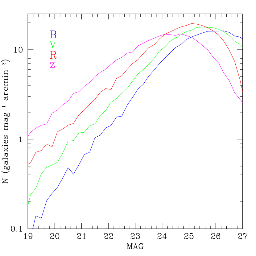
Figure 2: DLS $N(mag_{iso})$ for BVRz.

In order to have a realistic galaxy luminosity function, $N(mag)$, we start our simulations from R-band magnitudes of 87260 objects detected in one of our $\sim 40^{\prime}\times 40^{\prime}$ Deep Lens Survey sub-fields (Wittman et al. 2002). The typical BVRz magnitude distributions for the DLS are shown in Figure 2. We take this magnitude as the true ($\neq observed$) R-band magnitude of a new object to be simulated. From the $P(T|m_{0})$ prior we select a SED, and from $P(z|T,m_{0})$ we choose a ${z_{\rm input}}$ redshift for the galaxy. The resulting “true” redshift distribution in the simulations is shown in Figure 3. This distribution has a larger tail to high redshift than usually found in the literature (e.g. LeFevre et al 2005) and can be approximately described as $z^{2}exp\big{(}-1(\frac{z}{0.05})^{0.54}\big{)}$. Magnitudes (with or without noise) in any other photometric bands can then be computed. We use BPZ itself to compute synthetic colors, so there is no issue of minor differences in the k-corrections, priors, etc. We assume that there are only six SED‘s of galaxies in the universe and make no attempt to introduce template noise in these simulations. We then perform three sets of simulations in the BVRz filter set of the DLS. In the first simulation (SIM1) we assume perfect, infinite S/N photometry. In the second set of simulations (SIM2) we successively degrade the S/N  of the photometry but maintain constant the S/N of all galaxies in all 4 bands (same magnitude error for all galaxies in all 4 bands). In the third simulation (SIM3), we reproduce the S/N distribution and completeness of the DLS.

3.1 SIM1

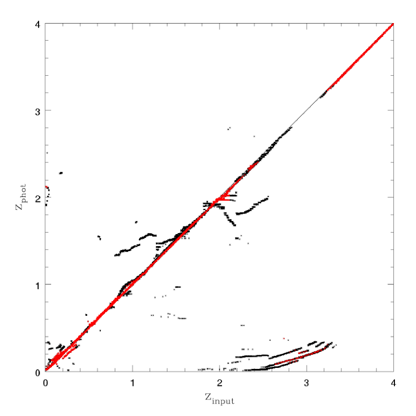
Figure 4: ${z_{\rm phot}}-{z_{\rm spec}}$ scatter-plot for SIM1 (no photometry noise). Galaxies with $ODDS>0.9$ are in red. See first line of Table 1 for statistics.

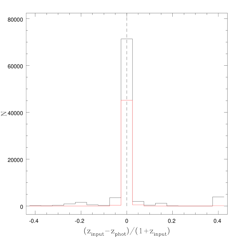
Figure 5: Histogram of ${\Delta z}$ for the simulation in Figure 4. The distribution of galaxies with $ODDS>0.9$ is shown in red. The outermost bins show the integrated counts of all objects with $|{\Delta z}|>0.4$.

The first simulation (SIM1) has perfect photometry and represents the best possible case. The ${z_{\rm phot}}-{z_{\rm spec}}$ scatter-plot for this simple simulation is shown in Figure 4, and the distribution of ${\Delta z}\equiv{{z_{\rm spec}}-{z_{\rm phot}}\over 1+{z_{\rm spec}}}$ is shown in Figure 5. Note that Figure 4 contains 87260 objects, distributed in redshift according to Figure 3, and that the ${z_{\rm phot}}={z_{\rm spec}}$ line is saturated with objects. It is clear from Figure 5 that the majority of objects have $|{\Delta z}|\sim 0.0$. Table 1 indicates: (1) signal-to-noise of photometry (same in all bands); (2) fraction of galaxies with $|{\Delta z}|<0.5$; (3) mean ${\Delta z}$ for galaxies with $|{\Delta z}|<0.5$; (4) rms in ${\Delta z}$ for galaxies with $|{\Delta z}|<0.5$; (5) fraction of objects with $ODDS>0.9$; (6) fraction of objects with $ODDS>0.9$ and $|{\Delta z}|<0.5$; (7) mean ${\Delta z}$; and (8) rms in ${\Delta z}$ for these galaxies.

There are still catastrophic outliers, despite being the best possible case in terms of noise, perfectly known templates, etc. This is because each galaxy is assigned a single ${z_{\rm phot}}$ based on the peak of its PDF. Consider a degeneracy such that the same colors come from SED  A at $z_{1}$ or SED  B at $z_{2}$. In the absence of priors, this would result in a PDF with two equal peaks. Now add priors encoding our astrophysical knowledge, such as that an apparently bright galaxies are likely to be at low redshift, or that ellipticals are rare at high redshift. This usually helps select the correct peak, but sometimes it will select the wrong peak because unlikely events do happen: some high-redshift galaxies are bright, or are ellipticals. As noted above, this ignores the full PDF, which may be broad or multi-modal in a way that is consistent with the true redshift. As our purpose is only to establish SIM1 as a baseline for investigating the impact of photometric S/N, we do not pursue this here.

3.2 SIM2

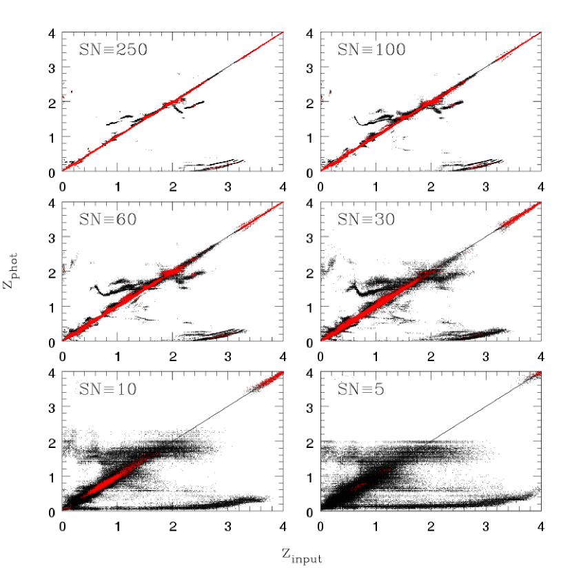
Figure 6: ${z_{\rm phot}}-{z_{\rm spec}}$ scatter-plot for simulations with realistic magnitude and redshift distributions, but uniform and progressively greater photometry noise (SIM2). In each panel all galaxies have the same S/N  in BVRz. From top-left to bottom-right: SN=250, 100, 60, 30, 10, 5. See Table  1 for statistics.

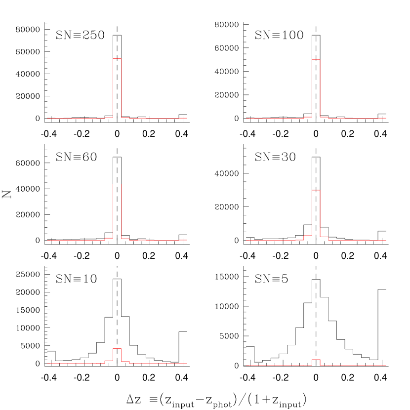
Figure 7: Histogram of ${\Delta z}$ for objects shown in Figure 6 (SIM2).

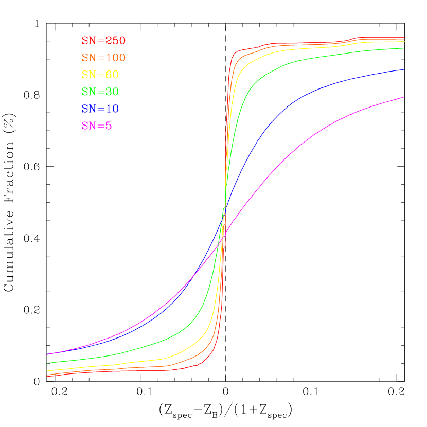
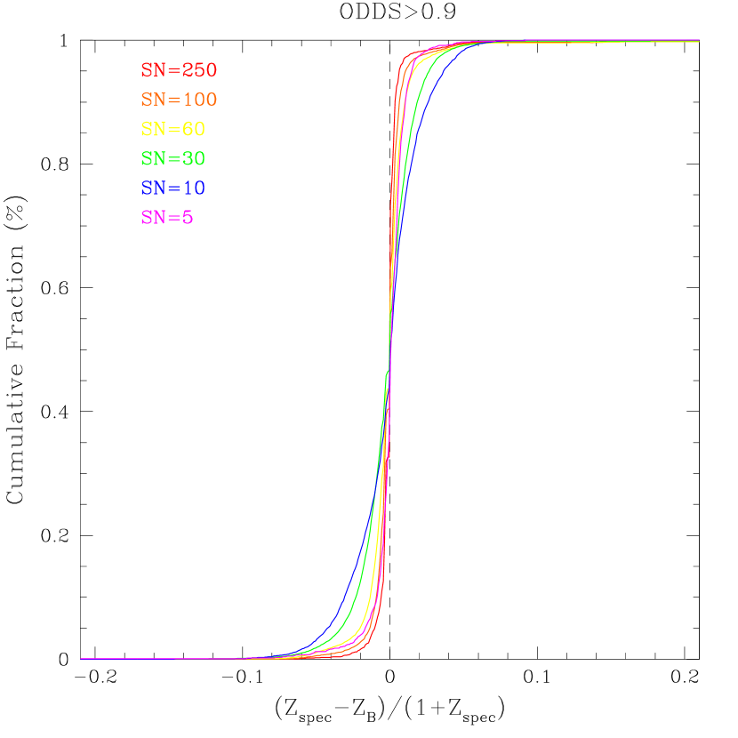
Figure 8: Cumulative fraction of objects with ${\Delta z}$ smaller than a given value. Red line indicates the simulation in which all galaxies have been set to have $SN=250$ in all BVRz; orange indicates a simulation with $SN=100$; and so on. Right panel shows all galaxies, and left panel shows galaxies with $ODDS>0.9$. Note that only 6.4% and 1.2% respectively of objects with $SN=10,5$ have $ODDS>0.9$.

In the second set of simulations (SIM2) we degrade the initially perfect photometry in SIM1 successively to S/N  of 250 ($R\sim 20.5^{m}$ in the DLS, and the magnitude limit of the spectroscopic sample presented in Section 4), 100, 60, 30, 10 and 5, and repeat the analysis at each step. In these unrealistic simulations all galaxies have the same photometric S/N  in all bands. The scatter-plots are shown in Figure 6, and ${\Delta z}$ distributions are shown in Figure 7. We also present the cumulative fraction of objects with ${\Delta z}$ smaller than a given value, as a function of ${\Delta z}$ (Figure 8). This plot has several advantages. First, multiple simulations can be over-plotted without obscuration. Second, the asymmetry in the distribution of ${\Delta z}$ is easily read off by looking at the fraction with ${\Delta z}<0$ (dashed vertical line). Third, the fraction of outliers can also be directly read off the plot at any ${\Delta z}$. The left panel of Figure 8 shows the cumulative fraction for all objects, while the right panel shows $ODDS>0.9$ galaxies. The number of galaxies in the right panel is smaller than the number in the left (see Table 1) but the accuracy of photo-zs is clearly better.

Because all realizations of SIM2 have the redshift distribution shown in Figure 3, even if all galaxies have colors measured at very high S/N , some objects will have degenerate colors and the sample will contain some fraction of catastrophic outliers. Spectroscopic samples typically have a much lower mean redshift than these simulations, so catastrophic outliers are likely to be underrepresented in direct ${z_{\rm phot}}-{z_{\rm spec}}$ comparisons, if the full photometric sample is very deep.

Table 1 presents the statistics for the SIM2 objects shown in Figures 6,  7 and  8. Clearly, the precision of photometric redshifts is a strong function of photometric S/N. BPZ’s ODDS parameter is very effective at removing outliers, and almost 100% of the objects with $ODDS>0.9$ have $|{\Delta z}|<0.1$ regardless of S/N (right panel in Figure 8). However, the fraction of objects with $ODDS>0.9$ decreases dramatically with decreasing S/N.

Performance is, counter-intuitively, slightly worse for the infinite S/N galaxies in SIM1 than for the high S/N galaxies in SIM2. This is because the priors have too much power when there is no noise in color space, and is not of concern in more realistic situations.

3.3 SIM3

The third simulation has the same S/N  distribution and completeness as the DLS data. Again, the priors used assure that the galaxy type mixture and redshift distribution should be close to the real universe. The idea is to measure how well we can recover true ${z_{\rm input}}$ redshifts for a realistic photometric data set. This simulation is still optimistic because no template noise is added—we derive colors from the same six templates used in the determination of photometric redshifts. The effect of template noise will be presented in the real data analysis in Section 4.

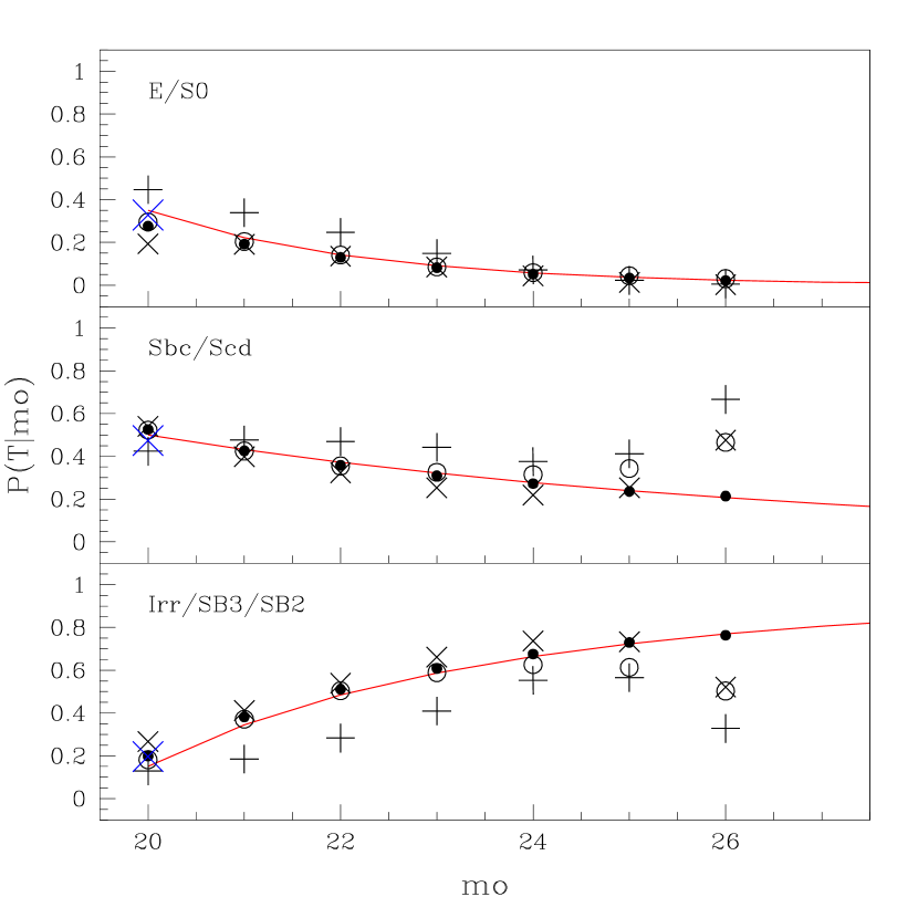
Figure 9: Galaxy type fraction as a function of magnitude, $P(T|m_{0})$. The solid red lines indicate BPZ’s priors used in the simulations of Section 3 and shown previously in Figure 1. The “$+$” and “$\times$” symbols indicate fraction of galaxies classified by BPZ as E, Sbc/Scd, or Im/SB3/SB2 in two DLS fields of $40^{\prime}\times 40^{\prime}$ each. The “$+$” field, with higher fraction of ellipticals, contains the galaxy cluster Abell 781, while the “$\times$” represents a more typical “blank” field. The simulation input distribution is indicated by solid circles, which by definition agree with the red line, while the open circles indicate the BPZ type classification of these objects. The blue “$\times$” represents the SHeLS spectroscopic sample.

As a sanity check we compare the BVz magnitude distributions of our SIM3 simulation with the observed $N(mag)$ and find good agreement. The R magnitude distribution is by definition the same within the added photometric noise. We also compare the distribution of BPZ galaxy types in DLS fields with the one derived from the SIM3 simulation and find very good agreement. Figure 9 shows the galaxy type fraction as a function of magnitude for two $40^{\prime}\times 40^{\prime}$ DLS fields. The field with the higher fraction of ellipticals contains the richness class 2 galaxy cluster Abell 781 at $z=0.298$ (“$+$”), and the other is a more typical “blank” field (“$\times$”). The simulation input distribution is indicated by solid circles, which by definition agree with the red line, and the output BPZ types are indicated by open circles. SIM3 and data show the same magnitude dependence.

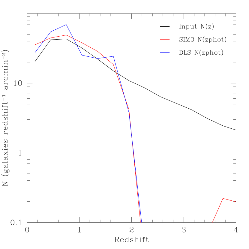
Figure 10: Photometric redshift distributions for the DLS (blue) and SIM3 (red). The input $N(z)$ for the simulations is shown in black.

A third sanity check is a comparison between the redshift distribution derived in SIM3 and $N(z)$ for the entire DLS survey. Figure 10 shows both distributions and also the input redshift distribution used in the simulations (same as shown in Figure 3). The agreement is pretty good. The mean density of galaxies with photometric redshifts of any quality is $47/arcmin^{2}$ and $11\%$ of those objects have $ODDS>0.9$.

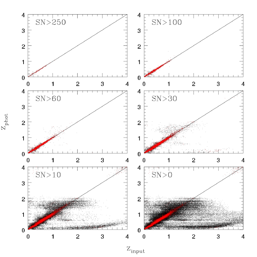
Figure 11: ${z_{\rm phot}}-{z_{\rm spec}}$ scatter-plot for simulations with realistic magnitude, redshift, and S/N distributions (SIM3). Upper left panel shows all galaxies with very high S/N  (small number density and mostly at low redshift) while lower right panel includes all galaxies in the simulation. From upper left to lower right: (1) galaxies with $SN>250$; (2) $SN>100$; (3) $SN>60$; (4) $SN>30$; (5) $SN>10$; and (6) $SN=All$.

The photometric redshift performance on SIM3 is shown on Figures 11,  12 and 13, just as in Figures 6,  7 and 8 for SIM2. The summary statistics for SIM3 are presented in Table 2. As in SIM2, the precision of photometric redshifts is a strong function of S/N, and ODDS does a good job of cleaning up, at the cost of losing many low S/N galaxies.

There are two notable differences with SIM2. First, in SIM3, there is a realistically strong correlation between high S/N and bright magnitudes. A bright magnitude implies a strong prior (most bright galaxies are at low redshift), whereas a faint galaxy has a weak prior (it could be at any redshift). The high S/N galaxies in SIM2 were (artificially) at all magnitudes, and therefore had generally looser priors. Therefore, the highest S/N galaxies in SIM3 do better than those in SIM2. We can see the effect of the tight priors directly by comparing the $S/N=250$ line of Table  1 ($\sigma_{{\Delta z}}=0.042$ after clipping 4% which had $|{\Delta z}|>0.5$) with that of Table 2 ($\sigma_{{\Delta z}}=0.031$ with no need to clip any outliers). This difference vanishes when low S/N galaxies from SIM3 are included.

In fact, the $S/N=5$ galaxies in SIM2 outperform the $S/N>5$ galaxies in SIM3, despite the latter cut being only a lower bound. This is due to the second salient difference between SIM2 and SIM3: A given S/N in SIM2 describes each galaxy in each band. In SIM3, the S/N varies with filter in a realistic way, and the cut applies to R band. Most galaxies will have lower S/N in other bands. For $S/N=30$ in R, the median $S/N$ in B, V, and z over the whole sample is 10, 18, and 10 respectively.

What S/N is required for good photometric redshift performance? First, consider performance without any ODDS cut. At each step in Table 2 from $S/N>100$ to $S/N>10$, there is a 30–50% increase in $\sigma_{{\Delta z}}$, so there is no natural breakpoint. $\sigma_{{\Delta z}}$ appears to stop this dramatic growth when stepping down from $S/N>10$ to $S/N>5$, but this is likely an artifact of clipping at $|{\Delta z}|>0.5$, which is roughly three times the clipped rms at that point. Even at $S/N>10$, $\sigma_{{\Delta z}}$ may be artificially low due to clipping, as more than 10% of galaxies were clipped. Most survey users would find the precision offered by the $S/N>30$ cut acceptable, but the $S/N>10$ cut unacceptable. If we set $\sigma_{{\Delta z}}=0.1$ as the limit of acceptability, we find an S/N cut at 17 is required.

Now consider using the ODDS cut at 0.9. $\sigma_{{\Delta z}}$ is always 0.04 or less, regardless of S/N. We suspect that for a given $\sigma_{{\Delta z}}$, the ODDS cut will provide more galaxies than the S/N cut, because ODDS responds to the properties of the color space as well as to S/N. For example, high-precision S/N is not required if the galaxy is in a distinctive region of color space. In addition, ODDS can take proper account of different S/N in different bands, which a simple S/N cut in R does not. We investigate this by finding the ODDS cut which yields the same $\sigma_{{\Delta z}}$ as the $S/N>30$ cut (0.076). We find that $ODDS>0.57$ is required, which yields 30% of all detected galaxies, vs. the 13% yielded by the S/N cut.

We repeat this procedure for $\sigma_{{\Delta z}}=0.1$. The required ODDS cut is $>0.40$, yielding 45% of all detected galaxies, while the required S/N cut at 17 yields only 26% of detected galaxies.

These fractions can all be read off Figure 14 which summarizes the results from SIM3. The three left panels in Figure 14 show: (1) the cumulative fraction of objects with S/N greater than a given value; (2) mean ${\Delta z}$; and (3) $\sigma_{{\Delta z}}$ for these objects. The three right panels are the same but for a cut in $ODDS$.

In short, we recommend an ODDS cut. We recognize that an ODDS cut is not easy to incorporate into survey forecasts of the number of usable galaxies. Detailed simulations for a given filter set and depth as a function of wavelength must be performed. However, we hope that the above numbers can serve as a rough guide for translation between photometric redshift precision, S/N threshold, and number of usable galaxies.

4 Data

We take photometric data from the DLS BVRz full-depth images in fields with spectroscopic redshifts from the Smithsonian Hectospec Lensing Survey (SHeLS, Geller et al.  2005), and from the Caltech Faint Galaxy Redshift Survey (CFGRS, Cohen et al.  1999) surveys. Here, by definition, template noise is present. In Sections 4.3 and 4.4 we present the spectroscopic data and the photometric redshift accuracy for these two samples, but before that we present our methodology for color measurement (Section 4.1), and template optimization (Section 4.2).

4.1 Measuring Colors

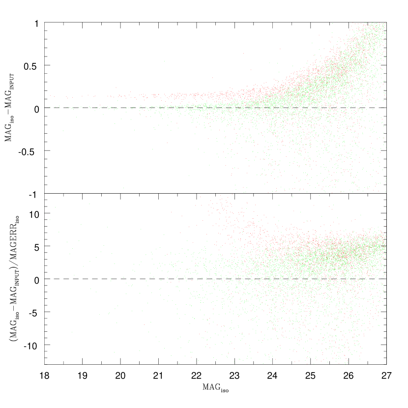
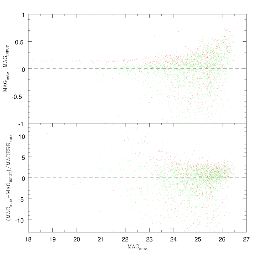
Figure 15: Magnitude errors of synthetic De Vaucouleurs (red) and exponential disk (green) galaxies added to DLS R-band images. Left panels show the SExtractor $MAG_{ISO}$ results while right panels indicate comparisons to SExtractor $MAG_{AUTO}$. Top: $\Delta{MAG}\equiv MAG-MAG_{input}$ vs. $MAG$. Bottom: $\Delta{MAG}/MAGerr$ vs. $MAG$.

We performed simulations to determine the best photometry method in the face of different point-spread function (PSF) sizes in the different filters. We added galaxies with De Vaucouleurs (elliptical) and exponential disk (spirals) light profiles to the DLS BVRz data using standard IRAF-Artdata routines, ran SExtractor (Bertin & Arnouts 1996) and measured colors with many different types of magnitudes. Figure 15 shows the results for galaxies added to the R images. The B, V and z results are qualitatively the same, but because of differences in S/N and PSF there is a shift in the magnitude axis, and slightly different scatter. The left panels show the results using $MAG_{iso}$ and right panels show $MAG_{auto}$. The top panels show the difference between measured $MAG$ and input $MAG_{input}$. De Vaucoleurs galaxies are measured to be $\sim 0.15^{m}$ fainter than their true magnitudes both by $MAG_{iso}$ and $MAG_{auto}$. The bottom panels show the distribution of $(MAG-MAG_{input})/MAGerr$ as a function of magnitude. As noted by Benitez et al.  (2004), $MAG_{auto}$ gives better results for magnitudes, but for photometric redshifts we are interested in good colors as deep as possible.

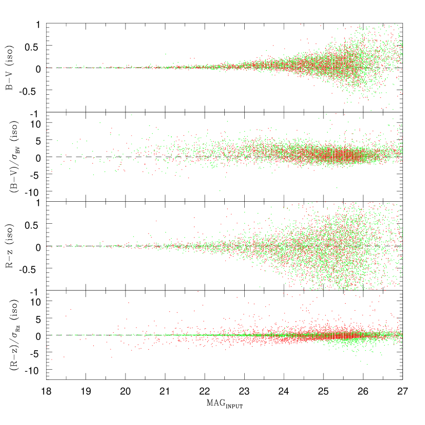
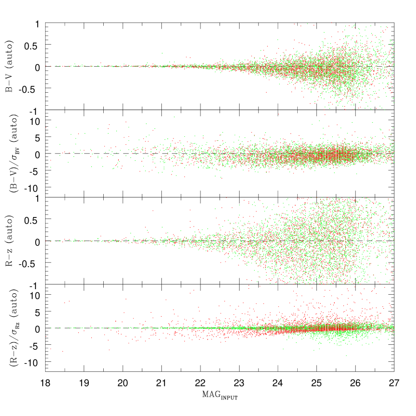
Figure 16: Color errors of synthetic De Vaucouleurs (red) and exponential disk (green) galaxies added to DLS images. Left panels show the SExtractor $MAG_{ISO}$ results while right panels indicate comparisons to SExtractor $MAG_{AUTO}$. The four panels in each column show different color combinations.

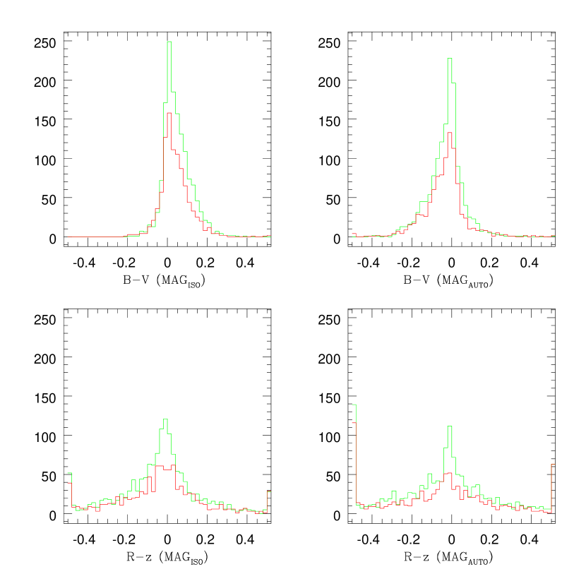
Figure 17: Distribution of colors derived from $MAG_{ISO}$ and $MAG_{AUTO}$ for zero-color synthetic De Vaucouleurs (red) and exponential disk (green) galaxies added to DLS data. Here we show galaxies brighter than $24.5^{m}$ which corresponds to ${S/N}\sim 10$ in BVR, but goes down to ${S/N}\sim 3$ in z. The edge bins indicate the number of objects out of the limits of the plot.

Figures 16 and 17 show the distribution of color errors, which, for photometric redshifts, are more important than magnitude errors. Again, $MAG_{iso}$ is on the left and $MAG_{auto}$ on the right. The systematic magnitude errors tend to cancel when considering colors, and $MAG_{iso}$ is now slightly better. It is important to note that the errors in magnitude errors are not driven by faint galaxies, and that in fact the discrepancies between real and estimated colors errors are significantly worse for bright objects.

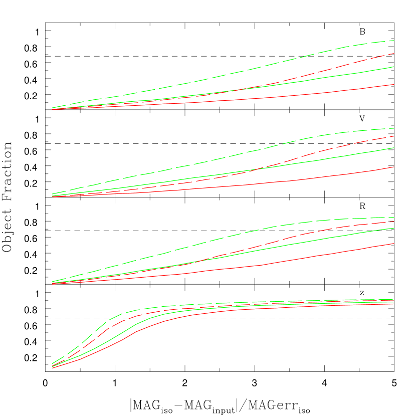
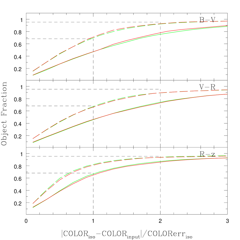
Figure 18: Cumulative fraction of objects as function of $\Delta_{MAG}/MAGerr_{ISO}$ and $\Delta_{COLOR}/COLORerr_{ISO}$. Red lines represent galaxies with a De Vaucouleurs light profile, and green lines represent galaxies with an exponential disk. The dashed lines indicate the cumulative fraction after an ad hoc increase in the measured magnitude errors. The augmented errors guarantee that $\sim 68(95)\%$ of the galaxies have colors within $1(2)\sigma$. A much larger increase would be needed in order to have $\sim 68(95)\%$ of galaxies with measured magnitudes within $1(2)\sigma$.

In summary, $MAG_{iso}$ gives slightly more precise colors at a given magnitude. This translates to more galaxies being detected above a given S/N threshold, providing another benefit. However, for either $MAG_{auto}$ or $MAG_{iso}$, the error estimates provided by SExtractor are optimistic, especially at the bright end. The solid lines in Figure 18 show the cumulative fraction of objects as a function of magnitude and color error, normalized by the nominal error from SExtractor. Much less than $68(95)\%$ of the galaxies have actual errors within the nominal 1(2)$\sigma$ magnitude error. Actual color errors are closer to nominal, but still optimistic. (Caveat: unlike most real galaxies, the simulated galaxies had zero color.) From this analysis we determine an ad hoc correction to the magnitude errors estimated by SExtractor: we first multiply $MAGerr_{iso}$ by $1.5$, and then add in quadrature an error of $0.02^{m}$. The dashed lines in both panels of Figure 18 show the results of this correction. This single correction puts the 68th and 95th percentiles of all the color distributions in the correct place, with the exception of the 68th percentile of $R-z$ color. This adjustment to the magnitude errors should in principle depend on galaxy color, but we found that variations about this correction made little difference in the results.

We performed all the real-data tests in this paper with both $MAG_{iso}$ and $MAG_{auto}$. The differences in the results were very minor, except that more galaxies were detected at a given S/N with $MAG_{iso}$, and about 20% more survived the ODDS cut with $MAG_{iso}$. We therefore adopt $MAG_{iso}$ for the remainder of this paper.

Another factor to consider is the quality of the survey’s photometric calibration, which was determined by observations of standard stars in Landolt’s (1992) fields during photometric nights. The R and V DLS bands are very similar to Landolt’s filter transmissions and yield accurate calibration. The DLS B-band however differs significantly from Landolt’s and requires a color term correction which decreases the accuracy of calibration in this band. Also, the DLS z-band photometry derived from Sloan Digital Sky Survey standards (Smith et al.  2002) is also not as good as R and V. For this reason we add an extra $0.01^{m}$ to the magnitude error measurements in B and z bands.

4.2 Template Optimization

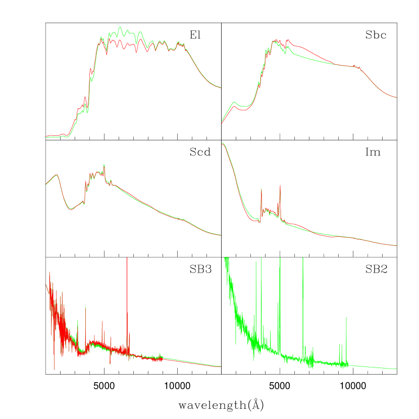
Figure 19: Optimized SED templates are shown in red, and the original templates are in green. SB2 template was kept unchanged.

We use spectroscopic redshifts and the DLS photometry to empirically correct the BPZ set of templates and to test our filter+instrument response knowledge with the methodology described in Ilbert et al. 2007. We find optimized templates for El, Sbc, Scd, Im, and SB3 SEDs. The SB2 template was left unchanged because there were not enough galaxies of this type to fit a correction. The biggest modifications were found for the El SED, which shows a less strong 4000Å  break in the optimized template; and for the Sbc SED, which has a stronger 4000Å  break than in the original BPZ template (See Figure 19). Because most of our galaxies are at low redshift, we cannot constrain the longest and shortest SED wavelengths and therefore we force them to agree with the initial templates.

4.3 Comparison with Spectroscopic Data: SHeLS Survey

The SHeLS survey has a limiting magnitude of $R=20.3$, so that the DLS photometry, which is complete to about five magnitudes fainter, is very high S/N. Being a bright magnitude-limited survey, SHeLS contains overwhelmingly low-redshift ($z<0.6$) galaxies. However, our subsample of 1,000 was chosen to provide a nearly uniform redshift distribution so that characterization accuracy would be roughly redshift-independent. At a given redshift, selection was random.

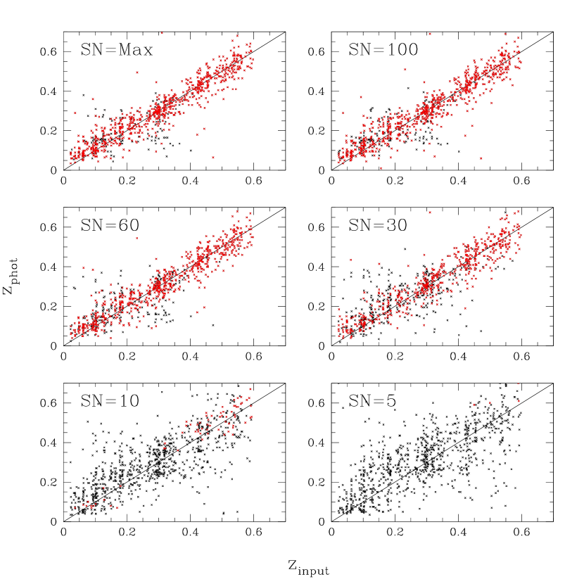
Figure 20: ${z_{\rm phot}}-{z_{\rm spec}}$ scatter-plot for 860 objects with spectroscopic redshifts from the SHeLS survey in the DLS survey. Top-left panel shows the results when the maximum S/N photometry is used. The five other panels (from top-right to bottom=right) show the results with progressively greater photometry noise: ${S/N}=100,60,30,10,5$. See Table 3 for statistics.

We further cut the sample, requiring ${S/N}>100$ in the R band, and excluding objects in exclusion zones around bright stars, or with saturated pixels in any band, or with SExtractor $flags\geq 4$ (compromised photometry). The final sample contains 860 galaxies. The top left panels of Figures 20 and  21 show the ${z_{\rm phot}}-{z_{\rm spec}}$ scatter-plot, and ${\Delta z}$ distribution for the maximum S/N  photometry. The distribution of galaxy types assigned by BPZ to this spectroscopic sample is in agreement to the type distribution of all galaxies at $R=20\pm 0.5^{m}$ in the entire DLS survey, suggesting that the spectroscopic sample is representative of galaxies at this magnitude.

The SHeLS sample is expected to show evidence of template noise and have somewhat higher $\sigma_{{\Delta z}}$ than the bright end of SIM3, and this is in fact observed. Objects with ${S/N}>100$ in SIM3 have $\sigma_{{\Delta z}}=0.037$, and $89.4\%$ of the galaxies have $ODDS>0.9$ with $\sigma_{{\Delta z}}=0.026$. For the SHeLS survey, $\sigma_{{\Delta z}}=0.050$, and $85.6\%$ have $ODDS>0.9$ with $\sigma_{{\Delta z}}=0.044$. The difference suggests a template noise of $\sigma_{{\Delta z}}\sim 0.035(1+z)$ which is smaller than the $0.065(1+z)$ estimated by Fernandez-Soto et al.  (1999) for galaxies in the Hubble Deep Field, but expected given the much lower redshift of galaxies in the SHeLS survey.

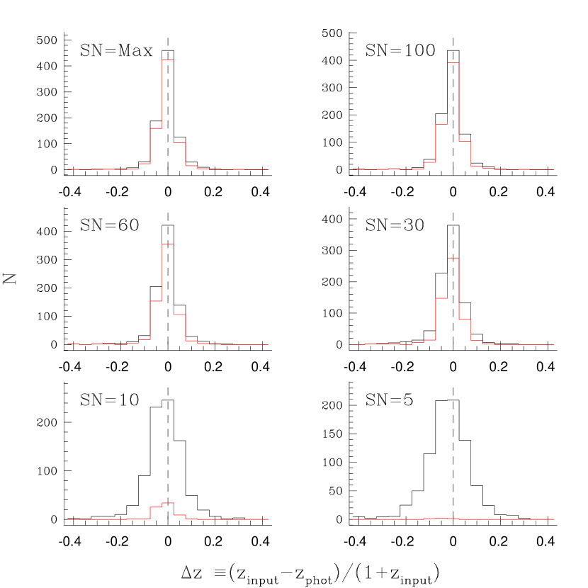
Figure 21: Histogram of $\delta z$ for for objects shown in Figure 20.

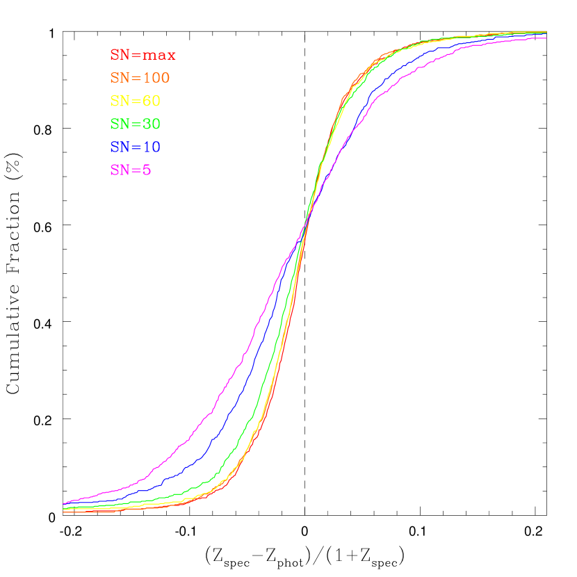
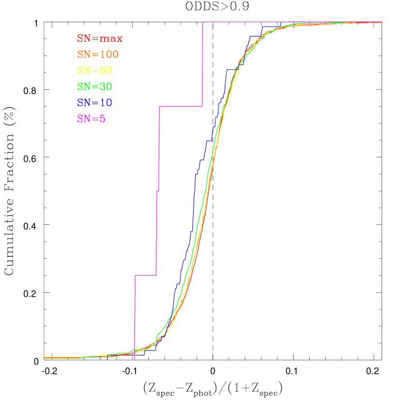
Figure 22: Cumulative fraction of objects as a function of ${\Delta z}$. Red lines shows the cumulative fraction for maximum S/N photometry in the SHeLS survey; orange shows the fraction when objects are noised up simulate $SN=100$ in BVRz; and so on. Right panel shows all galaxies, and left panel shows galaxies with $ODDS>0.9$.

We now degrade the photometry successively to ${S/N}=100,60,30,10,5$ in all bands. If a galaxy has, for example ${S/N}=50$ in the B band, its magnitude and magnitude error are left unchanged in this band for the simulations with ${S/N}=100$ and ${S/N}=60$, but noise is added to the other ones. The ${z_{\rm phot}}-{z_{\rm spec}}$ scatter-plots are shown in Figure 20. ${\Delta z}$ distributions are shown in Figure 21, and cumulative fraction as a function of ${\Delta z}$ is shown in Figure 22. Statistics in different S/N regimes are presented in Table 3. The trends with S/N which were observed in the simulations are reproduced here.

Because the magnitude prior remains tight despite the S/N degradation, we observe lower $\sigma_{{\Delta z}}$ at the low S/N end of the SHeLS simulations than is observed for SIM2 at the same S/N. At ${S/N}=10$, $\sigma_{{\Delta z}}=0.080$, and $8.3\%$ of galaxies in the SHeLS survey have $ODDS>0.9$, while $\sigma_{{\Delta z}}=0.121$, and $6.4\%$ of the have $ODDS>0.9$ for the SIM2 galaxies.

The effectiveness of the ODDS cut is again evident. The fraction of galaxies passing this cut at low S/N is less than in SIM3 because the data here are uniformly at low S/N, whereas for SIM3 the given S/N is a lower limit. The fraction with $ODDS>0.9$ at low S/N is more directly comparable with, and more consistent with, the fractions in SIM2, which were also at constant S/N.

4.4 Comparison with Spectroscopic Data: CFGRS Survey

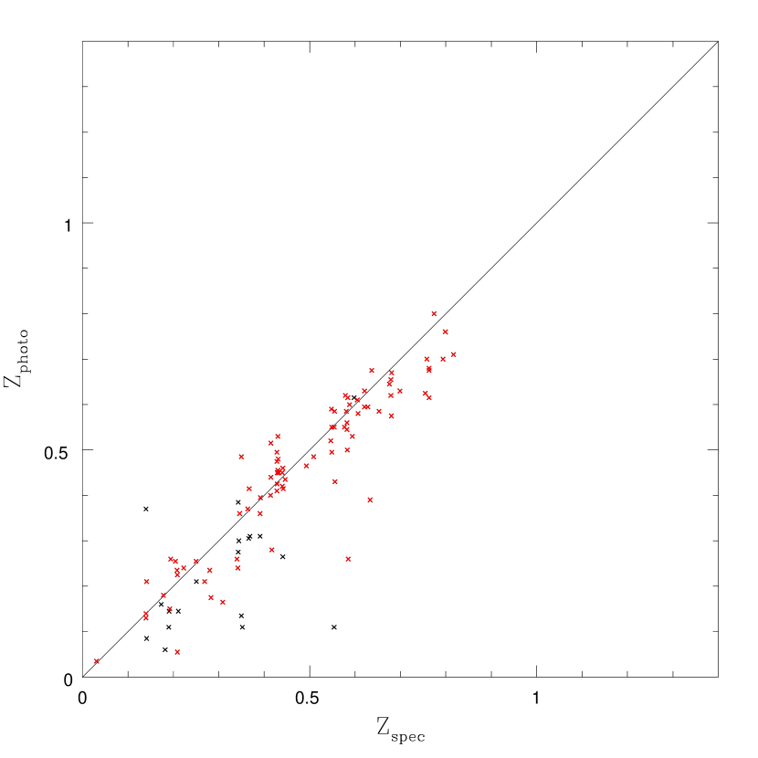
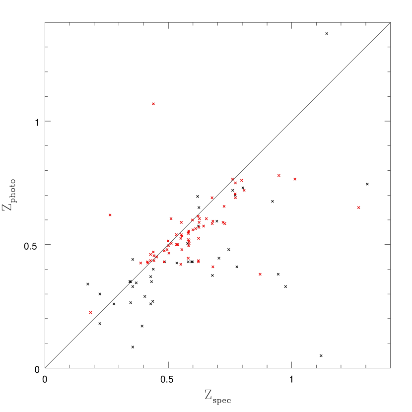
Figure 23: ${z_{\rm phot}}-{z_{\rm spec}}$ scatter-plot for 222 objects with spectroscopic redshifts from the CFGRS survey. The sample was subdivided in two: left, ${S/N}>106$; right,${S/N}<106$. In red, we show objects with $ODDS>0.9$.

The CFGRS (Cohen et al.  1999) survey is about $2^{m}$ deeper than SHeLS and therefore the DLS photometry is not as high S/N. We select galaxies with quality=1 (multiple spectral features, Cohen et al.  1999) spectroscopic redshifts and divide the data in 2 equally sized subsamples of 111 galaxies each: one with galaxies of photometric ${S/N}(R)>106$, and another with ${S/N}(R)<106$. Note that the signal-to-noise in the low S/N  sample is still fairly high, with 28 being the lowest value, and a median of 69, but the difference in the quality of photometric redshifts is clear. Figure 23 shows the ${z_{\rm phot}}-{z_{\rm spec}}$ scatter-plot for the two sub-samples. For the high S/N sample, ${\Delta z}=0.027\pm 0.084$, and ${\Delta z}=0.021\pm 0.060$ if we exclude 1 catastrophic outlier with $|{\Delta z}|>0.5$. For the lower S/N sample, ${\Delta z}=0.033\pm 0.166$, and ${\Delta z}=0.041\pm 0.095$ if we exclude 2 objects with $|{\Delta z}|>0.5$. However this includes the effect of different redshift ranges. To isolate the S/N effect, we compute results using only galaxies between $0.4<z<0.9$, where both samples have a significant density of sources. For the high S/N sample we find ${\Delta z}=0.020\pm 0.056$, and for the lower S/N sample, we find ${\Delta z}=0.034\pm 0.073$. No objects with $|{\Delta z}|>0.5$ are found in this redshift range.

5 Selection in Galaxy Type and Redshift Range

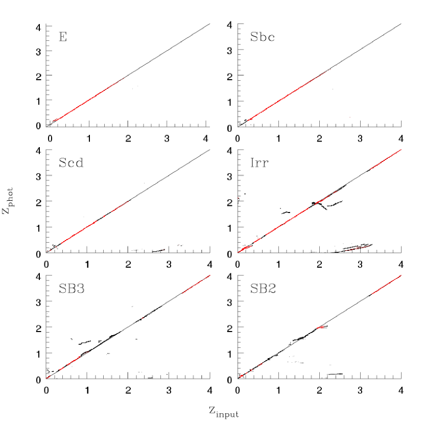
Figure 24: ${z_{\rm phot}}-{z_{\rm spec}}$ scatter-plot for SIM1 subdivided according to BPZ galaxy type ($T_{B}$). Galaxies with $ODDS>0.9$ are in red.

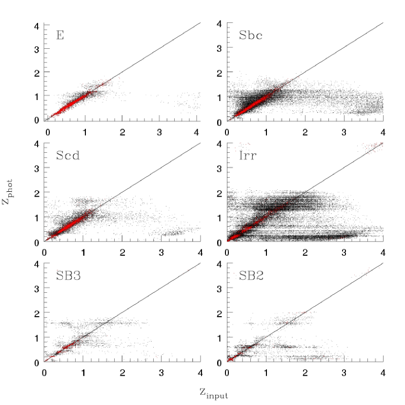
Figure 25: ${z_{\rm phot}}-{z_{\rm spec}}$ scatter-plot for SIM3 subdivided according to BPZ galaxy type ($T_{B}$). Galaxies with $ODDS>0.9$ are in red.

Figure 9 suggests that faint Irr/SB2/SB3 galaxies are often misclassified as Sbc/Scd. In this section we explore dependence on type in more detail. Figures 24,  25, and  26 show the ${z_{\rm phot}}-{z_{\rm spec}}$ scatter-plot as a function of inferred BPZ galaxy type ($T_{B}$) for SIM1, SIM3, and the SHeLS galaxies respectively. Ellipticals form the tightest relation, while the redshift of irregular galaxies show a scatter more than twice as large. Figure 25 shows that some of the scatter in ellipticals must be due to misclassifications, because there are no E-type galaxies at $z\sim 3-4$ in the simulations.

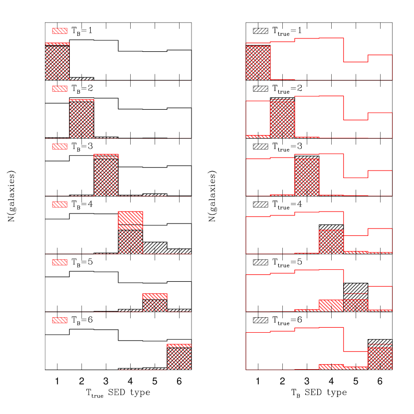
Figure 27: Input spectral type ($T_{true}$) vs. output BPZ type ($T_{B}$) for SIM3 galaxies with $S/N>30$. Types are: $1-E$; $2-Sbc$; $3-Scd$; $4-Irr$; $5-SB3$; $6-SB2$. In the left panels we select galaxies by $T_{B}$ (shaded red) and then look at their $T_{true}$ distribution (shaded black). The unshaded black histogram is the same in all plots and indicates the $T_{true}$ distribution. In the right panels, we select galaxies by their true type (shaded black) and then look at the $T_{B}$ distribution (shaded red). The unshaded red histogram indicates the $T_{B}$ distribution.

We look at type misclassification in SIM3 directly in Figures 27 and  28. The left column of panels shows the $T_{B}$ distribution for each of the true input types, with the true type distribution overlaid like a diagonal matrix in red to guide the eye. The right column of panels shows the true type distribution for each of the inferred types, with the inferred type distribution overlaid in red to guide the eye. The overall distribution of inferred (true) types is shown by the unshaded histogram which is repeated in each panel in the left (right) column. Figures 27 shows galaxies with ${S/N}\geq 30$ or $R\leq 23$. For example, the fourth panel down in the left column shows that galaxies classified as $T_{B}=4$ (Irr), have in fact almost the same probability of being of types 4, 5 or 6 (irregular or starburst). Likewise, starburst galaxies tend to be misclassified at irregulars even at high S/N.

The types in decreasing order of reliability are E, Sbc, Scd, Irr, SB3, and SB2. Type reliability translates to redshift reliability, because type misclassification usually implies a large, if not catastrophic, redshift error. These figures also demonstrate that although the ODDS cut appears to lose many high high-redshift galaxies and shrink the usable redshift range, in fact most of the “high-redshift” galaxies lost were type misclassifications, and therefore unreliable redshifts. Although the loss of these “high-redshift” galaxies is painful if one wants as large a redshift range as possible, it is necessary if one wants the sample to be reliable.

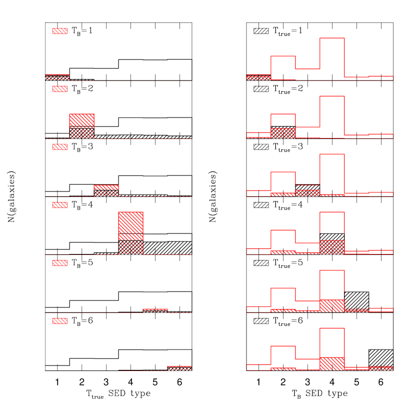
Figure 28: Same as Figure 27 but including galaxies with very low S/N (all detections). Black represents true galaxy types (input) and red indicates the $T_{B}$ classification.

In Figure 28 we extend the analysis to lower S/N galaxies, and include all “detected” galaxies. The rate of misclassification is much higher. The insertion of these objects in the sample creates new types of misclassification. For example, a fraction of type 1 (E) galaxies is assigned $T_{B}=2$ and vice-versa. Also, a significant fraction of types 4, 5, and 6 (irregular and starburst) are classified as types 2 or 3 (spirals).

6 Summary and Discussion

We have examined the dependence of photometric redshift performance on photometric S/N, using both simulations and data. For concreteness, we have used the DLS filter set, but the general trends should apply to any filter set. As a reminder, SIM2 simulated galaxies at a range of magnitudes drawn from the DLS photometry, but at a series of constant S/N levels, while SIM3 strongly couples magnitude and S/N as they are in the DLS photometry. Thus, bright is distinct from high S/N in SIM2 and in the noise-augmented SHeLS data because bright implies a more effective magnitude prior. An additional distinction between SIM3 and the other cases is that in SIM3 a given S/N cut is performed in R, and for most galaxies that implies a lower S/N in the other bands. For SIM2 and noise-augmented SHeLS data, a given S/N describes each galaxy in each filter.

We therefore expect the smallest $\sigma_{{\Delta z}}$ for very high S/N in SIM3, where the high S/N galaxies automatically have a tight magnitude prior. This is what is observed, $\sigma_{z}=0.031$ (0.037) for $S/N>250$ (100) in SIM3. Degeneracies in color space determine this performance limit, which is therefore highly filter-set dependent. However, it sets a baseline for what follows. At $S/N=100$ in the SHeLS data, $\sigma_{{\Delta z}}$ is about 35% larger than this baseline, suggesting a cosmic variance or template noise component of $\sigma_{{\Delta z}}=0.035(1+z)$. For SIM2, $\sigma_{{\Delta z}}$ is also about 32% larger than this baseline, presumably due to the looser magnitude priors on average. The deeper the survey, the less effective the magnitude prior, but performance is still quite good at this high S/N.

From this baseline, lowering the S/N smoothly increases $\sigma_{{\Delta z}}$ in SIM3, by 30–50% at each S/N step in Table 2 until $\sigma_{{\Delta z}}$ is no longer trustworthy due to the clipping at $|{\Delta z}|>0.5$. SIM2 degrades a bit more slowly due to its higher baseline $\sigma_{{\Delta z}}$. The noise-augmented SHeLS data degrades even more slowly, because magnitude priors always remain tight. Although $\sigma_{{\Delta z}}$ looks reasonably good even at $S/N=5$ for the degraded SHeLS data, we expect SIM3 to be more representative of true performance for this reason.

SIM3 indicates that without an ODDS cut, $S/N=17$ in R is likely to be the lowest acceptable S/N for reasonable photometric redshift performance ($\sigma_{{\Delta z}}=0.1$) in a survey with the DLS specifications (filter set and depth). A shallower survey may be able to go to lower S/N because the magnitude prior remains helpful to lower S/N in such a survey. In fact, the bright spectroscopic sample has $\sigma_{{\Delta z}}<0.1$ even at $S/N=5$, although we caution that this means $S/N=5$ in each filter. If we impose an ODDS cut rather than an S/N cut, $ODDS>0.40$ cut yields twice as many galaxies for the same $\sigma_{{\Delta z}}$ as the $S/N>17$ cut in R. Alternatively, survey users could use ODDS to decrease $\sigma_{{\Delta z}}$ while sacrificing galaxy counts; an $ODDS>0.9$ cut yields $\sigma_{{\Delta z}}=0.04$ averaged over all S/N.

We caution that there are some unmodeled effects which, if included, would result in a larger $\sigma_{{\Delta z}}$. First, template noise is not included in the simulations. $\sigma_{{\Delta z}}$ is larger in the SHeLS data than in SIM3 for $S/N>60$, which we attribute to template noise. Template noise becomes less important at lower photometric S/N, but the template noise in the SHeLS data may be artificially low. The templates were originally derived from bright galaxies like those in SHeLS, and further optimized on the SHeLS sample itself. A photometric sample which pushes to higher redshift may thus incur more template noise, and in fact Fernandez-Soto et al.  (1999) estimates $\sigma_{{\Delta z}}=0.065(1+z)$ for galaxies in the Hubble Deep Field.

Second, because galaxy counts are rising beyond the limiting magnitude for detection, an additional source of photometry noise must be taken into account. A source detected at S/N of a few is much more likely to be an “up-scattered” fainter galaxy than a “down-scattered” brighter galaxy. As pointed out by Hogg & Turner (1998, hereafter HT98), this is distinct from Malmquist bias, which is the over-representation of high-luminosity galaxies in a flux-limited sample. Although the resulting bias can be computed and corrected for if the galaxy count slope is known, the additional photometric uncertainty is unavoidable. In fact, HT98 conclude that “sources identified at signal-to-noise ratios of four or less are practically useless.” This source of noise was not reproduced in our simulations, so extrapolation to $S/N<5$ would be extremely dangerous. Our results for $S/N=5$ are still valid if five is interpreted as the effective S/N in the presence of this additional source of noise. For the no-evolution, Euclidean slope of $q=1.5$, the HT98 formulae indicate that this requires a detection at $S/N=5.64$. For $S/N=10$ and higher, the corrections are very small.

In addition to these dependences on S/N, several other lessons can be drawn:

• When forecasting photometric redshift performance for a survey, it is important to include realistic photometry errors.

• Estimating photometric redshift performance with spectroscopic samples can lead to optimistic results if the spectroscopic sample is not representative of the photometric sample. If the spectroscopic sample is brighter, matching the S/N is easily accomplished by adding photometry noise, but accounting for the larger redshift range of the photometric sample requires detailed modeling which must account for cosmic variance.

• The BPZ $ODDS$ parameter is very effective at identifying photometric redshifts which are likely to be poor. An $ODDS$ cut is more efficient than an S/N cut, because $ODDS$ takes account of the looser photometry requirements in distinctive regions of color space. Still, our simulations and artificially noisy data show that of the galaxies with $ODDS<0.9$, the ones with poor photometric redshifts may be in the minority. The tradeoff between $ODDS$ cut and usable numbers of galaxies must be assessed in light of the specific science goal. For example, if the science analysis weights each galaxy by its photometric S/N, a strict $ODDS$ cut may cut most of the galaxies but not most of the total weight. For weak lensing, shape noise limits the maximum weight of a galaxy, so a strict $ODDS$ cut may cut most of the weight. Finally, biases must be considered, as ellipticals are overrepresented in the set of galaxies with high $ODDS$. This may not affect weak lensing but will be important for studies of galaxy evolution and baryon acoustic oscillations.

We also explored cutting in type (as identified by BPZ) and redshift range. As expected, ellipticals do better than any other type, but we found that the $ODDS$ cut was still useful for ellipticals. As long as the $ODDS$ cut was being used, other types could safely be used as well. Therefore, we recommend cutting on ODDS rather than type.

Figure 3: $N({z_{\rm input}})$ for simulations.

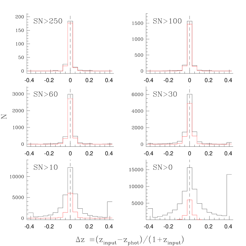
Figure 12: Histogram of ${\Delta z}$ for objects shown in Figure 11.

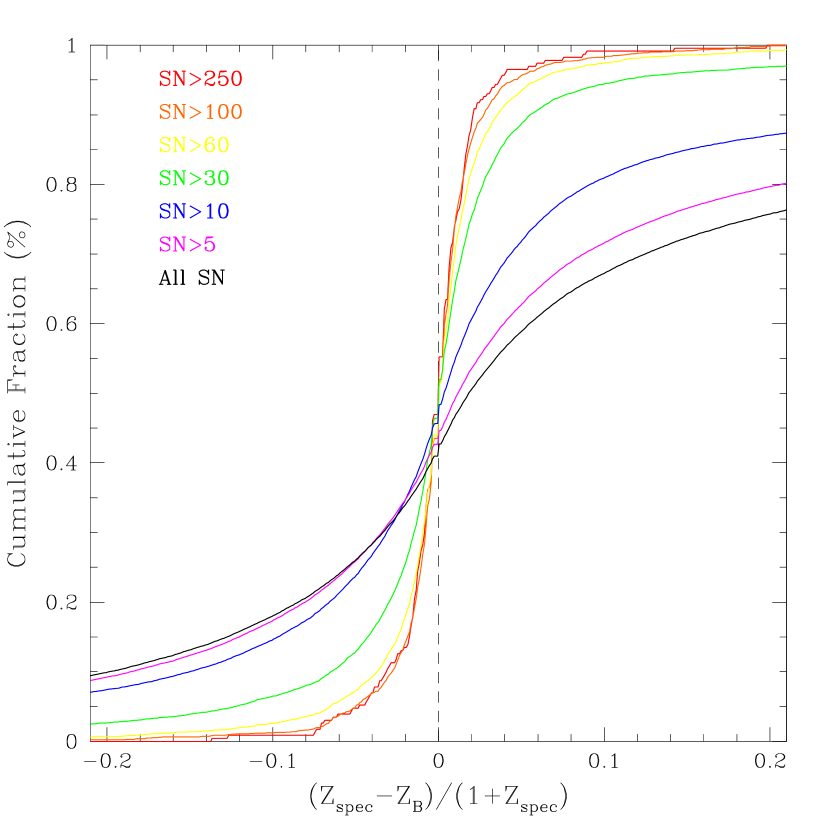
Figure 13: Cumulative fraction of objects with ${\Delta z}$ smaller than a given value for simulations with realistic magnitude and redshift distributions (SIM3). Red line shows the cumulative fraction for all objects with $SN(R)>250$; orange shows the fraction for all objects with $SN(R)>100$ (including those with $SN(R)>250$); and so on. Right panel shows all galaxies, and left panel shows galaxies with $ODDS>0.9$.

Figure 14: Left: Cumulative fraction of objects with S/N greater than a given value, mean ${\Delta z}$, and $\sigma_{{\Delta z}}$. Right: same as left panels for objects with $ODDS$ greater than a given value. Solid line indicates all objects and dashed lines shows $|{\Delta z}|<0.5$.

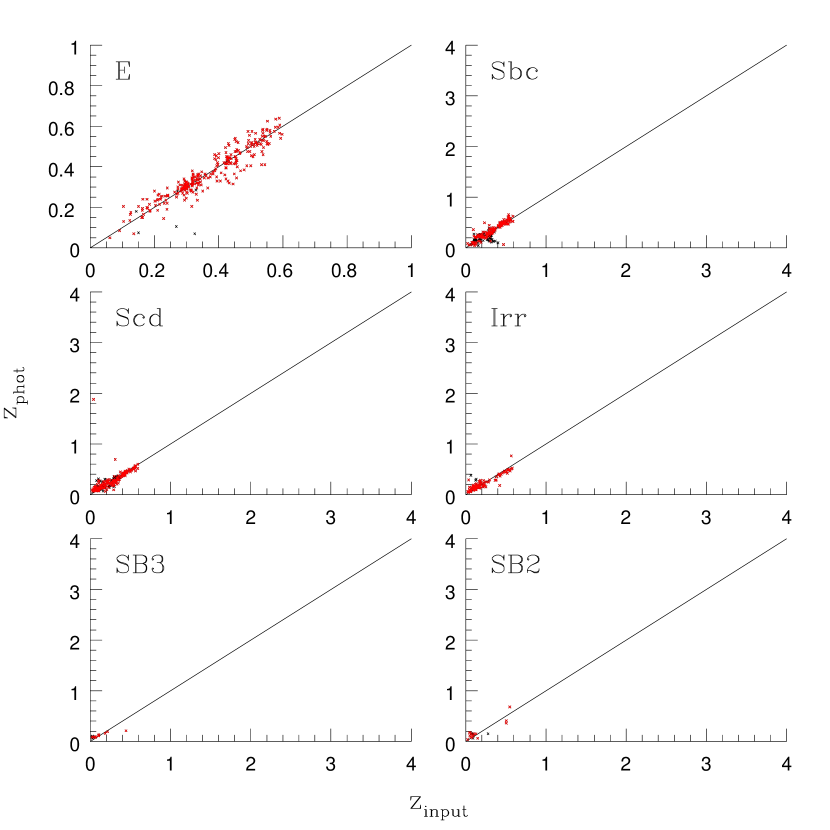
Figure 26: ${z_{\rm phot}}-{z_{\rm spec}}$ scatter-plot subdivided according to BPZ galaxy type ($T_{B}$) for 860 objects with spectroscopic redshifts from SHeLS. Galaxies with $ODDS>0.9$ are in red.

Table 1: Galaxies with Fixed Signal-to-Noise (SIM1 & SIM2)

SN	$|{\Delta z}|\leq 0.5$			$ODDS>0.9$
	$|{\Delta z}|\leq 0.5\over All$(%)	$\bar{{\Delta z}}$	$\sigma({\Delta z})$	$ODDS>0.9\over All$(%)	$|{\Delta z}|\leq 0.5~{}\&~{}ODDS>0.9\over ODDS>0.9$(%)	$\bar{{\Delta z}}$	$\sigma({\Delta z})$
Inf (SIM1)	95.3	-0.008	0.051	53.4	99.7	-0.000	0.006
250 (SIM2)	96.0	-0.005	0.042	64.2	99.8	-0.000	0.009
100 (SIM2)	95.5	-0.007	0.049	60.7	99.7	-0.000	0.012
60 (SIM2)	94.7	-0.010	0.062	54.4	99.7	-0.001	0.015
30 (SIM2)	92.5	-0.014	0.085	40.6	99.9	-0.002	0.020
10 (SIM2)	87.6	-0.007	0.121	6.4	100.0	-0.001	0.023
5 (SIM2)	84.7	0.019	0.151	1.2	99.9	0.001	0.012

Table 2: Galaxies in DLS like simulations (SIM3)

SN(R)	$|{\Delta z}|\leq 0.5$			$ODDS>0.9$
	$|{\Delta z}|\leq 0.5\over All$(%)	$\bar{{\Delta z}}$	$\sigma({\Delta z})$	$ODDS>0.9\over All$(%)	$|{\Delta z}|\leq 0.5~{}\&~{}ODDS>0.9\over ODDS>0.9$(%)	$\bar{{\Delta z}}$	$\sigma({\Delta z})$
$>250$	100.0	-0.001	0.031	90.9	100.0	-0.001	0.021
$>100$	100.0	0.001	0.037	89.4	100.0	0.000	0.026
$>60$	99.7	-0.000	0.050	82.6	100.0	0.000	0.030
$>30$	97.8	-0.004	0.076	67.0	99.6	-0.001	0.036
$>10$	89.3	-0.004	0.125	23.5	99.3	-0.001	0.040
$>5$	85.0	0.008	0.154	14.1	99.3	-0.001	0.040
All	83.6	0.018	0.170	11.9	99.3	-0.001	0.040

Table 3: Galaxies with Spectroscopic Redshifts from the SHeLS Survey

SN	$|{\Delta z}|\leq 0.5$			$ODDS>0.9$
	$|{\Delta z}|\leq 0.5\over All$(%)	$\bar{{\Delta z}}$	$\sigma({\Delta z})$	$ODDS>0.9\over All$(%)	$|{\Delta z}|\leq 0.5~{}\&~{}ODDS>0.9\over ODDS>0.9$(%)	$\bar{{\Delta z}}$	$\sigma({\Delta z})$
Max	99.9	-0.005	0.050	85.6	99.9	-0.006	0.044
100	99.8	-0.006	0.050	83.0	99.9	-0.007	0.045
60	99.8	-0.006	0.054	76.9	99.7	-0.006	0.045
30	100.0	-0.012	0.061	62.9	100.0	-0.010	0.046
10	100.0	-0.016	0.080	8.3	100.0	-0.015	0.038
5	99.8	-0.021	0.090	0.5	100.0	-0.061	0.035

References

- Abdalla et al. (2007) Abdalla, F. B., Amara, A., Capak, P., Cypriano, E. S., Lahav, O., & Rhodes, J. 2007, ArXiv e-prints, 705, arXiv:0705.1437
- Benitez (2000) Benitez, N. 2000, ApJ, 536, 571
- Bertin & Arnouts (1996) Bertin, E., & Arnouts, S. 1996, A&AS, 117, 393
- Bolzonella et al. (2000) Bolzonella, M., Miralles, J.-M., & Pelló, R. 2000, A&A, 363, 476
- Cohen et al. (1999) Cohen, J. G., Hogg, D. W., Pahre, M. A., Blandford, R., Shopbell, P. L., & Richberg, K. 1999, ApJS, 120, 171
- Connolly et al. (1995) Connolly, A. J., Csabai, I., Szalay, A. S., Koo, D. C., Kron, R. G., & Munn, J. A. 1995, AJ, 110, 2655
- Csabai et al. (2000) Csabai, I., Connolly, A. J., Szalay, A. S., & Budavári, T. 2000, AJ, 119, 69
- Dickinson (1998) Dickinson, M. 1998, The Hubble Deep Field, 219
- Fernández-Soto et al. (1999) Fernández-Soto, A., Lanzetta, K. M., & Yahil, A. 1999, ApJ, 513, 34
- Fernández-Soto et al. (2001) Fernández-Soto, A., Lanzetta, K. M., Chen, H.-W., Pascarelle, S. M., & Yahata, N. 2001, ApJS, 135, 41
- Fernández-Soto et al. (2002) Fernández-Soto, A., Lanzetta, K. M., Chen, H.-W., Levine, B., & Yahata, N. 2002, MNRAS, 330, 889
- Geller et al. (2005) Geller, M. J., Dell’Antonio, I. P., Kurtz, M. J., Ramella, M., Fabricant, D. G., Caldwell, N., Tyson, J. A., & Wittman, D. 2005, ApJ, 635, L125
- Hogg et al. (1998) Hogg, D. W., et al. 1998, AJ, 115, 1418
- Hogg & Turner (1998) Hogg, D. W., & Turner, E. L. 1998, PASP, 110, 727
- Huterer et al. (2006) Huterer, D., Takada, M., Bernstein, G., & Jain, B. 2006, MNRAS, 366, 101
- Ilbert et al. (2006) Ilbert, O., et al. 2006, A&A, 457, 841
- Landolt (1992) Landolt, A. U. 1992, AJ, 104, 340
- Le Fèvre et al. (2005) Le Fèvre, O., et al. 2005, A&A, 439, 845
- Ma et al. (2006) Ma, Z., Hu, W., & Huterer, D. 2006, ApJ, 636, 21
- Smith et al. (2002) Smith, J. A., et al. 2002, AJ, 123, 2121
- Wittman et al. (2002) Wittman, D. M., et al. 2002, Proc. SPIE, 4836, 73
- Zhan & Knox (2006) Zhan, H., & Knox, L. 2006, ApJ, 644, 663