Hall field induced magnetoresistance oscillations of a two-dimensional electron system

Abstract

We develop a model of the nonlinear response to a DC electrical current of a two dimensional electron system(2DES) placed on a magnetic field. Based on the exact solution of the Schrödinger equation in arbitrarily strong electric and magnetic fields, and separating the relative and guiding center coordinates, a Kubo-like formula for the current is worked out as a response to the impurity scattering. Self-consistent expressions determine the longitudinal and Hall components of the electric field in terms of the DC current. The differential resistivity displays strong Hall field-induced oscillations, in agreement with the main features of the phenomenon observed in recent experiments.

PACS numbers: 73.43.-f,73.43.Qt,73.40.-c,73.50.Fq

I Introduction

Recently, non-equilibrium magnetotransport in high mobility two-dimensional electron systems (2DES) has acquired great experimental and theoretical interest. Microwave-induced resistance oscillations (MIRO) attaining zero resistance states were discovered a few years ago Zudov et al. (2001); Mani et al. (2004); Zudov et al. (2003) in 2DES subjected to microwave irradiation and moderate magnetic fields, corresponding to very high Landau levels (LL$s$). The phototoresistance exhibits strong oscillations periodic in $\epsilon=\omega/\omega_{c}$, where $\omega$ and $\omega_{c}$ are the microwave and cyclotron frequencies. Our current understanding of this phenomenon rest upon models that predict the existence of negative-resistance states yielding an instability that rapidly drive the system into a zero resistance state Andreev et al. (2003). Two distinct mechanism for the generation of negative resistance states are known, one is based in the microwave induced impurity scattering Ryzhii (1970); Durst et al. (2003); Lei and Liu (2003); Shi and Xie (2003); Vavilov and Aleiner (2004); Torres and Kunold (2005), while the second is linked to the modifications of the distribution produced by the microwaves and inelastic processes Dmitriev et al. (2003, 2005); Robinson et al. (2003). Similar to MIRO are magnetoresistance oscillations induced by the combined effects of microwave irradiation and periodic potential modulation Dietel et al. (2005); Torres and Kunold (2006); Yuan et al. (2006).

More recently, Hall field-induced resistance oscillations (HIRO) have been observed in high mobility samples in response to a strong DC electric current Yang et al. (2002); Bykov et al. (2005). The HIRO oscillations are periodic in inverse magnetic field, with the resistance maxima appearing at integer values of the dimensionless parameter $\epsilon=\omega_{H}/\omega_{c}$. The Hall frequency $\omega_{H}=\gamma\left(2\pi/n_{e}\right)^{1/2}J_{x}/e$, is associated to the energy $\hbar\omega_{H}=\gamma R_{c}\,E_{y}^{cl}$; where the the classical Hall electric field is given by $E_{y}^{cl}=BJ_{x}/en_{e}$, $R_{c}$ is the cyclotron radius of the electrons at the Fermi level, and $\gamma\sim 1.63\,\,to\,\,2.18$. These results were confirmed in the recent experiment by Zhang $et\,al.$ Zhang et al. (2007a), with a determination of the parameter $\gamma\sim 1.9$. Additionally in this work another notable nonlinear effect was found: in the regime of separated LL$s$ a relative weak DC current induces a dramatic reduction of the resistivity. Although MIRO and HIRO are basically different phenomena, both rely on the commensurability of the cyclotron frequency with a characteristic parameter, $\omega$ and $\omega_{H}$ respectively. The study of HIRO permits to analyze resistivity as a function of $\epsilon$ when both $\omega_{c}$ and $\omega_{H}$ are varied over a wide range of frequencies. Instead the MIRO studies are carried out performing $\omega_{c}$-sweeps at fixed $\omega$, because the experimental difficulty in implementing $\omega$-sweeps. Other interesting examples of nonlinear magnetotransport experiments combine DC and AC excitations Bykov et al. (2005); Zhang et al. (2007b).

Some theoretical studies of the nonlinear transport properties under DC exitations have recently appeared. In the work of Vavilov $et\,al.$ Vavilov et al. (2006) the nonlinear magnetotransport effects are related to changes of the electron distribution function induced by the DC electric field. On the other hand, the work of Lei Lei (2007) the impurity scattering processes are analyzed utilizing a semiclassical method in which the evolution of the CM velocity operator and relative electron energy are obtained from the Heisenberg operator equations, and the CM electron coordinate and velocity are treated classically. The aim of this work is to develop a model to describe the nonlinear response to a DC electrical current of a 2DES placed on a magnetic field. Our model is based on the exact solution of the Shrödinger in arbitrarily strong magnetic and electric fields. It is convenient to separate the electron coordinate in its relative $\boldsymbol{R}$ and guiding center $\boldsymbol{X}$ coordinates. Although the relative and guiding center coordinates commute; the $R_{x}$ and $R_{y}$ relative coordinates satisfy a non-commutative algebra (and similarly for the $X$ and $Y$ projections of the relative coordinates). These properties are exploited to work out a Kubo-like formula for the conductivity as a response to randomly distributed impurities. Self-consistent expressions determine the longitudinal and Hall components of the electric field in terms of the DC current density $J_{x}$. The Hall electric field $E_{y}$ is given by the dominant classical Hall contribution $E_{y}^{cl}=BJ_{x}/en_{e}$, plus an small quantum correction $\Delta E_{y}$. The differential resistance displays a strong oscillatory behavior resulting from current assisted electron scattering producing both intra-LL and inter-LL transitions. The results of the present work taken together with those of Lei Lei (2007) prove that the properties of HIRO oscillations in the overlapping LL$s$ region ($\epsilon>1$), as well as the strong resistance reduction in the separated LL regime can be both explained by a DC-current induced impurity scattering mechanism.

II Model

The goal of this work is to study the nonlinear response to a DC electrical current density ($J_{x}$) of a 2DES placed in a magnetic field. The electrons are subjected both to a magnetic $\boldsymbol{B}=\left(0,0,B\right)$ and an in-plane electric $\boldsymbol{E}=\left(E_{x},E_{y},0\right)$ fields. Additionally the effects of impurity scattering potential $V$ are included; hence the dynamics is governed by the Hamiltonian

$$H=H_{\{B,E\}}+V\,,$$ (1)

where

$$H_{\{B,E\}}=\frac{1}{2m^{*}}\boldsymbol{\Pi}^{2}+e\boldsymbol{E}\cdot\boldsymbol{x}\,,$$ (2)

includes the interaction with the magnetic and electric fields, the covariant momentum is $\boldsymbol{\Pi}=-i\hbar\boldsymbol{\nabla}+e\boldsymbol{A}$. The impurity potential is decomposed in terms of its Fourier components

$$V\left(\boldsymbol{r}\right)=\sum_{i}^{N_{i}}\int\frac{d^{2}q}{\left(2\pi\right)^{2}}V\left(q\right)\exp\left[i\boldsymbol{q}\cdot\left(\boldsymbol{r}-\boldsymbol{r}_{i}\right)\right]\,,$$ (3)

where $\boldsymbol{r}_{i}$ is the position of the $i$th impurity and $N_{i}$ is the number of impurities. The explicit form of $V\left(q\right)$ depends on the nature of the scatterers. For short-range neutral impurities Torres and Kunold (2005): $V\left(q\right)=2\pi\hbar^{2}\alpha/m^{*}$, where $\alpha$ is the scattering length, and the impurity density is related to the electron mobility according to the relation $\alpha^{2}n_{imp}=e/(4\pi^{2}\hbar\mu)$. Instead, in the case of a $2D$ screened Coulomb potential: $V\left(q\right)=\frac{\pi\hbar^{2}q_{TF}}{m^{*}}e^{-qd}/\left(q_{TF}+q\right)$, where $d$ is the thickness of the doped layer and $q_{TF}=e^{2}m^{*}/\left(2\pi\epsilon_{0}\epsilon_{b}\hbar^{2}\right)$; in this case the relation of the impurity density to the electron mobility is approximated as $n_{imp}=8e(k_{F}d)^{3}/(\pi\hbar\mu)$.

A planar electron performs cyclotron and drifting motion in magnetic and electric fields. It is then convenient to decomposed the electron coordinate $\boldsymbol{r}$ into the guiding center $\boldsymbol{X}=(X,Y)$, and the the relative coordinate $\boldsymbol{R}=(R_{x},R_{y})$, $i.e.$: $\boldsymbol{r}=\boldsymbol{X}+\boldsymbol{R}$, where $\boldsymbol{R}=(-\Pi_{y}/eB\,,\,\Pi_{x}/eB)$. The commutation relations are

$$\left[R_{x},R_{y}\right]=\frac{i\hbar}{eB}\,,\hskip 39.83368pt\left[X,Y\right]=-il_{B}^{2}\,,\hskip 39.83368pt\left[X_{i},R_{j}\right]=0\,,$$ (4)

with $l_{B}^{2}=\hbar/eB$. With this decomposition the $X$ and $Y$ coordinates become noncommutative (similarly for $R_{x}$ and $R_{y}$); however the guiding center and the relative coordinates are independent variables.

For an arbitrary orientation of the electric field $\boldsymbol{E}=E\left(\cos\theta,\sin\theta,0\right)$, the Hamiltonian $H_{\{B,E\}}$ can be exactly diagonalized if the vector potential is selected in the gauge: $\boldsymbol{A}=B\left(y\,\sin^{2}\theta\,,\,-\,x\,\cos^{2}\theta,\,0\right)$. The spectrum and eigenstates are given by

$${\cal E}_{\{\mu,k\}} = \hbar\omega_{c}\left(\frac{1}{2}+\mu\right)+eEl_{B}k-\frac{(eEl_{B})^{2}}{2\hbar\omega_{c}}\,,$$

$$\Psi_{\mu,k} = \frac{1}{\sqrt{2^{\mu}\mu!\sqrt{\pi}l_{B}}}\,\exp\{-ik\,\eta\}\,\exp\{-(\xi-\xi_{c})^{2}/2l_{B}^{2}\}\,H_{\mu}\left[(\xi-\xi_{c})/l_{B}^{2}\right]\,,$$ (5)

here $\xi=x\cos\theta+y\sin\theta$, and $\eta=-x\sin\theta+y\cos\theta$ are the longitudinal and transverse coordinates (with respect to the electric field); $\xi_{c}=\frac{el_{B}^{2}E}{\hbar\omega_{c}}-l_{B}k$, and $H_{\mu}$ represent the Hermite polynomials. The index $k$ is the eigenvalue of the transverse $-X\sin\theta+Y\cos\theta$ center of guide coordinate.

We now turn to the calculation of the current density. The velocity of the center guide coordinates are obtained from the Heisenberg operator equations using the total Hamiltonian in Eq. (1):

$$\dot{X}=\frac{i}{\hbar}\left[H,X\right]=\frac{E_{y}}{B}-\frac{l_{B}^{2}}{\hbar}\,\frac{\partial V}{\partial y}\,,\hskip 71.13188pt\dot{Y}=\frac{i}{\hbar}\left[H,Y\right]=-\frac{E_{x}}{B}+\frac{l_{B}^{2}}{\hbar}\,\frac{\partial V}{\partial x}\,.$$ (6)

The current density is computed from the impurity and thermal average $\left\langle\boldsymbol{J}\right\rangle=e\langle\mathrm{Tr}\left[\rho\left(t\right)\boldsymbol{V}\right]\rangle$ of the center of guide velocity $\boldsymbol{V}=(\dot{X},\dot{Y})$, weighted with the density matrix that satisfies the von Neumann equation

$$i\frac{\partial}{\partial t}\rho=\left[H_{0}+V,\rho\right]\,.$$ (7)

We shall now derive the Kubo-Greenwood formula for the current within the framework of the linear response theory with respect to the impurity potential. The electric field effects are exactly taken into account through the wave function solution given in Eq. (II). The Hamiltonian is split into a unperturbed part $H_{\{B,E\}}$ and into the perturbation $V(\boldsymbol{r})\,\exp\left(-\delta|t|\right)$; notice that we added to the impurity potential a term $\exp\left(-\delta|t|\right)$, with $\delta$ representing the rate at which the perturbation is turned on and off. The density is similarly decomposed as $\rho=\rho_{0}+\Delta\rho$, where the unperturbed density matrix takes the form $\rho_{0}=\sum_{\alpha}f({\cal E}_{\alpha})|\alpha\rangle\langle\alpha|$; where $f$ is the Fermi distribution function. Following the usual procedure of the linear response formalism, the matrix elements of $\Delta\rho$, in the base given by states in Eq. (II), are worked out as

$$\langle\mu,k|\,\Delta\rho\,|\nu,k^{\prime}\rangle=\langle\mu,k|\,V\,|\nu,k^{\prime}\rangle\left(f_{\nu,k^{\prime}}-f_{\mu,k}\right)\,\frac{1}{{\cal E}_{\nu,k^{\prime}}-{\cal E}_{\mu,k}+i\delta}\,.$$ (8)

Combining the previous equations, and assuming randomly distributed impurities, the average current density is explicitly computed; as suggested by Eq. (6) the current is spplited in drifting and impurity scattering contributions:

$$J_{i}(\boldsymbol{E})=\epsilon_{ij}\,\frac{en_{e}}{B}E_{j}\,+\,J_{i}^{(imp)}(\boldsymbol{E})\,,\hskip 42.67912ptJ_{i}^{(imp)}(E_{x},E_{y})=\epsilon_{ij}\int\frac{d^{2}q}{(2\pi)^{2}}q_{j}F(\omega_{\boldsymbol{q}})\,,$$ (9)

here the function $F$ is given by

$$F(\omega_{q})=-\frac{en_{I}}{\hbar}\left|V\left(\boldsymbol{\boldsymbol{q}}\right)\right|^{2}\sum_{\mu,\nu}\left|D_{\mu,\nu}\left(\tilde{q}\right)\right|^{2}\left[f\left(E_{\mu}+\omega_{q}\right)-f\left(E_{\nu}\right)\right]\mathrm{Im}G\left(E_{\mu}+\omega_{q}-E_{\nu}\right)\\$$ (10)

and is evaluated at arbitrary values of the electric field through the argument dependence according to

$$\omega_{q}=el_{B}^{2}\left(q_{y}E_{x}-q_{x}E_{y}\right)\,.$$ (11)

The matrix elements $D_{\mu,\nu}$ are given by

$$D_{\mu,\nu}(\tilde{q})=\exp\left(-\frac{\left|\tilde{q}\right|^{2}}{2}\right)\left\{\begin{array}[]{ll}\tilde{q}^{\mu-\nu}\sqrt{\frac{\nu!}{\mu!}}L_{\nu}^{\mu-\nu}\left(\left|\tilde{q}\right|^{2}\right),&\mu\geq\nu,\\ \left(-{\tilde{q}}^{*}\right)^{\nu-\mu}\sqrt{\frac{\mu!}{\nu!}}L_{\nu}^{\nu-\mu}\left(\left|\tilde{q}\right|^{2}\right),&\mu\leq\nu,\\ \end{array}\right.$$ (14)

with $\tilde{q}=(q_{x}-iq_{y})/\sqrt{2}$ and $L_{\nu}^{\mu-\nu}\left(\left|\tilde{q}\right|^{2}\right)$ denotes the associated Laguerre polynomial.

A formal procedure to obtain the Green function requires a self-consistent calculation using the Dyson equation for the self-energy with the magnetic, impurity, phonon, and other scattering effects included. A detailed calculation of $Im\,G$ incorporating all these elements is beyond the scope of the present work. Instead we choose a gaussian-type expression for the the density of states. This expression can be justified within a self-consistent Born calculation that incorporates the magnetic field and disorder effects Ando and Uemura (1979); Gerhardts (1975a, b); Ando et al. (1982), hence the density of states for the $\mu$-Landau level is represented as

$$Im\,G\left(\omega_{\boldsymbol{q}}+E_{\nu}-E_{\mu}\right)=\sqrt{\frac{\pi}{2\Gamma^{2}}}\exp\left[-\frac{\left(\omega_{\boldsymbol{q}}+E_{\nu}-E_{\mu}\right)^{2}}{2\Gamma^{2}}\right],\quad\quad\Gamma^{2}=\frac{2\beta\hbar^{2}\omega_{c}}{\tau_{tr}}.$$ (15)

The parameter $\beta$ depends on the difference of the transport scattering time $\tau_{tr}$ obtained from the mobility and the single particle scattering time $\tau_{s}$. In the case of short-range scatterers $\tau_{tr}=\tau_{s}$ and $\beta=1$. In the case of long-range screened potential, $\beta_{\nu}$ depends on the filling factor $\nu$, $e.g.$ $\beta_{\nu=50}\approx 13.5$. Torres and Kunold (2005)

The current in Eq. (9) applies in general in the non-linear transport regimen, for an arbitrary strength of the DC electric field. The linear response regime is recovered if the function $F(\omega_{q})$ is expanded to first order in $E$ (the zero order term cancels because of the angular integration) to yield: $J_{x}=\sigma_{xx}\,E_{x}$ and $J_{y}=\sigma_{yy}\,E_{y}$, where

$$\sigma_{xx}=\sigma_{yy}=el_{B}^{2}\int\,\frac{d^{2}q}{(2\pi)^{2}}\,\,q_{y}^{2}\,\,\left(\frac{\partial F}{\partial\omega_{q}}\right)_{\omega_{q}=0}$$ (16)

and $\sigma_{xy}=\sigma_{yx}=en/B$.

Let us now consider the nonlinear transport regime. In a typical experimental configuration the electric field is not explicitly controlled, instead the longitudinal current $J_{x}$ is fixed to a constant value, while the transverse Hall current $J_{y}$ cancels. Consequently Eqs. (9) lead to the conditions

$$J_{x} =\hskip 8.5359pt\frac{en_{e}}{B}E_{y}+J_{x}^{(imp)}(E_{x},E_{y})\,,$$

$$0 =-\frac{en_{e}}{B}E_{x}+J_{y}^{(imp)}(E_{x},E_{y})\,.$$ (17)

They represents two implicit equation for the unknown $E_{x}$ and $E_{y}$; the equations can be solved following a self-consistent iteration. However, it is easily verified that for the conditions that apply in recent experiments, the solution of the previous equations simplify assuming that the following conditions $E_{x}\ll E_{y}$ and $J_{x}^{(imp)}\ll en_{e}E_{y}/B$ are simultaneously satisfied. It is then possible to explicitly solve for $E_{x}$ and $E_{y}$

$$E_{y} =\frac{B}{en_{e}}J_{x}-\frac{B}{en_{e}}J_{x}^{imp}(E_{x},E_{y})\approx\frac{B}{en_{e}}J_{x}-\frac{B}{en_{e}}E_{x}\left(\frac{\partial J_{x}^{imp}(E_{x},E_{y})}{\partial E_{x}}\right)_{(E_{x}=0,E_{y}=BJ_{x}/en_{e})}\,,$$ (18)

$$E_{x} =\frac{B}{en_{e}}J_{y}^{imp}(E_{x},E_{y})\approx\frac{B}{en_{e}}J_{y}^{imp}(E_{x}=0,E_{y}=BJ_{x}/en_{e})\,.$$ (19)

In order to derive the previous results we used the fact that $J_{x}^{imp}(E_{x}=0,E_{y})$ cancels because of the angular integration. Eq. (18) shows that the leading contribution to the Hall electric field is given by the classical result $E_{y}^{cl}=BJ_{x}/en_{e}$, however there is a correction $\Delta E_{y}$ given by the second term of the RHS. of Eq. (18). Utilizing Eqs. (9) the correction to the Hall electric field can be worked out as

$$\Delta E_{y}=\frac{\hbar\,E_{x}}{en_{e}}\int\,\frac{d^{2}q}{(2\pi)^{2}}\,\,q_{y}^{2}\,\,\left(\frac{\partial F}{\partial\omega_{q}}\right)_{\omega_{q}=\omega_{q}^{*}}\,,$$ (20)

where $E_{x}$ is determined by Eq. (19) and $\omega_{q}^{*}$ is given by

$$\omega_{q}^{*}=\frac{q_{x}J_{x}}{en_{e}}\,.$$ (21)

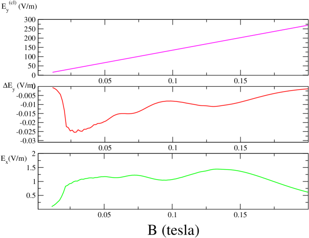
Figure 1: (color online) Induced electric Hall field: classical $E^{cl}_{y}\,(B)$ and quantum correction $\Delta E_{y}\,(B)$, and longitudinal electric field $E_{x}\,(B)$) calculated from Eqs. (18) and (19) at $J_{x}=0.8\,A/m$. The values of the other parameters are: $m^{*}=0.0635m_{e}$, $\mu=1.2\times 10^{7}\,cm^{2}/Vs$, $n_{e}=3.7\times 10^{11}cm^{-2}$, $T=1.5K$, and $\beta=5$.

Figure 1 shows the electric fields: $E_{y}^{cl}=BJ_{x}/en_{e}$, $\Delta E_{y}$, and $E_{x}$ as a function of the magnetic field for a fixed value of the longitudinal current. Notice that the conditions $\Delta E_{y}\ll E_{x}\ll E_{y}^{cl}$ hold in general, validating the assumed approximation. In fact it is verified that the approximated solutions in Eqs. (18) and (19) coincide with the self-consistent solutions that are obtained from Eqs. (II) with a better that $1\%$ precision.

Collecting the previous results, it follows that the Hall resistivity is well approximated by the expression

$$\rho_{xy}=\frac{E_{y}}{J_{x}}=\frac{B}{en_{e}}-\frac{BE_{x}}{en_{e}J_{x}}\left(\frac{\partial J_{x}^{imp}}{\partial E_{x}}\right)_{(E_{x}=0,E_{y}=BJ_{x}/en_{e})}\approx\frac{B}{en_{e}}\,.$$ (22)

Whereas the expression for the non-linear longitudinal resistivity is given as

$$\rho_{xx}=\frac{E_{x}}{J_{x}}=-\frac{B}{en_{e}J_{x}}\,\int\frac{d^{2}q}{(2\pi)^{2}}q_{x}F(\omega_{q}^{*})\,,$$ (23)

with $\omega_{q}^{*}$ given in Eq. (21). The differential resistivity is calculated as $r_{xx}=\partial\left(J_{x}\rho_{xx}\right)/\partial J_{x}$ yielding

$$r_{xx}=-\frac{\hbar B}{\left(en_{e}\right)^{2}}\int\frac{d^{2}q}{(2\pi)^{2}}q_{x}^{2}\left(\frac{\partial F}{\partial\omega_{q}}\right)_{\omega_{q}=\omega_{q}^{*}}\,.$$ (24)

Eqs. (9) for the nonlinear current together with the definitions in Eqs. (10-15) constitute the central result of the paper. They apply in general in the nonlinear regime in which both the longitudinal and Hall electric fields are arbitrarily strong. However, for the conditions that apply in the experiments of current interest, it is reasonable to consider the $E_{x}$ weak limit. Then, the Hall field is accurately approximated by the classical result $E_{y}=BJ_{x}/en_{e}$, whereas $\rho_{xx}$ and the differential resistivity are explicitly computed from Eq. (23) and Eq. (24) respectively.

In the work of Zhang $et\,al.$ Zhang et al. (2007a) the Hall frequency is defined $\omega_{H}=\gamma J_{x}\left(2\pi/e^{2}n_{e}\right)^{1/2}$. Here we assume that $\gamma=2$, this can be justified if we observe that the integral in Eq. (23) is evaluated in terms of the variable $\omega_{q}^{*}=q_{x}J_{x}/en_{e}$ and it is dominated by contributions of exchanged momentum in the region $q_{x}\approx 2k_{F}$. Recalling that $k_{F}=\sqrt{2\pi n_{e}}$, it yields $\omega_{H}=J_{x}\left(8\pi/e^{2}n_{e}\right)^{1/2}$. The dimensionless control parameter is then given by the ratio of the Hall to the cyclotron frequencies

$$\epsilon=\frac{\omega_{H}}{\omega_{c}}=\frac{2eE_{y}R_{c}}{\hbar\omega_{c}}\,,\hskip 56.9055ptR_{c}=\frac{v_{F}}{\omega_{c}}\,,$$ (25)

and it can be interpreted as the ratio of the work of the electric Hall field associated with the displacement of the guiding center of the cyclotron trajectory by $2R_{c}$ to the Landau energy $\hbar\omega_{c}$.

III Results

Results are presented for a 2DES $GaAs$ sample, with parameters corresponding to those reported in recent experiment of Zhang $et\,al.$ Zhang et al. (2007a): $m^{*}=0.0635m_{e}$ , electron mobility $\mu=1.2\times 10^{7}\,cm^{2}/Vs$ and density $n_{e}=3.7\times 10^{11}cm^{-2}$, and lattice temperature $T=1.5K$. For the impurities we consider an average of short- and long-range scatterers, selecting the parameter $\beta$ that appear in the Eq. (15) as $\beta=5.$

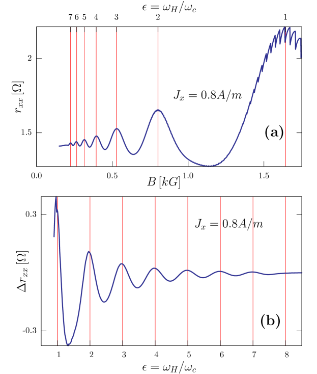
Figure 2: (color online) (a) Differential resistance $r_{xx}\,(B)$. (b) Correction to differential resistance $\Delta r_{xx}=r_{xx}-r_{xx}(J_{x}=0)$ versus $\epsilon=\omega_{H}/\omega_{c}$. The parameters have the same values as in Fig(1).

Fig. 2 (a) shows the differential resistance $r_{xx}$ as a function of the magnetic field $B$ for a fixed current density $J_{x}=0.8A/m$ $(\omega_{H}/2\pi\approx 65\,GHz)$. We observe clear differential magnetoresistance oscillations mounted on an offset of $1.41\Omega$ determined by the Drude contribution. At the top of this figure the values of $\epsilon=\omega_{H}/\omega_{c}$ are displayed, suggesting an oscillations period $\Delta\epsilon\sim 1$. To confirm these observations, in Fig. 2 (b) the Hal-field induced correction $\Delta r_{xx}=r_{xx}-r_{xx}(J_{x}=0)$ is plotted as a function of $\epsilon$. Magnetoresistance oscillations are clearly observed up to the seventh order. The first peak appears at $\epsilon\sim 0.95$, for higher $\epsilon$ oscillations the maxima occur at $\epsilon\approx j$, with $j$ an integer; while the minima are very close to $\epsilon\approx j+1/2$. These results are very similar to the experimental findings of Zhang $et\,al.$ Zhang et al. (2007a), although the localization of maxima (minima) close to integer (half integer) are here obtained when $\gamma=2$, whereas in that work they correspond to the selection $\gamma=1.9$. The amplitude of the differential resistance oscillations display a rapid decay as the magnetic field decreases. This decay can be parametrised by the Dingle factor $\delta=exp\left(-\pi/\omega_{c}\tau_{s}\right)$, this allow us to get an estimate of the single particle scattering time $\tau_{s}\approx 15\,ps$, that compares with the transport scattering time as $\tau_{s}/\tau_{tr}\approx 4.8$ ; in good agreement with the selected value $\beta=5$ .

To further support the previous results, we present in Figure 3 (a) a plot of $r_{xx}$ as a function of $1/B$ for various values of the longitudinal current density $J_{x}$. As expected each curve shows a different period as a function of $1/B$, though the decay of the oscillation amplitudes are well described by the same Dingle factor $\delta=exp\left(-\pi/\omega_{c}\tau_{s}\right)$, with $\tau_{s}\approx 15\,ps$. Notice that the all the curves share a maximum at $B=1/2.5KG$ given that $0.4\,A/m$, $0.6\,A/m$ and $0.8\,A/m$ are multiples of $0.2\,A/m$. Notwithstanding, when $\Delta r_{xx}$ is plotted as functions of $\epsilon$ in Fig. 3 (b), the positions of the maxima (minima) of the various curves draw close to integer (half integer) values of $\epsilon$.

The oscillation waveform can be more clearly appreciated in graphs in which $\epsilon$ varies performing current-sweepes at fixed $B$. In 4 (a) and (b) plots of $\Delta r_{xx}\,(\epsilon)$ are displayed for $B=416\,G$ and $B=732\,G$. We again observe that the first maxima appears at $\epsilon<1$, but as $\epsilon$ increases, the position of the maxima (minima) are localized very close to integer (semi-integer) values of $\epsilon$. The oscillation amplitude is almost constant, because the Dingle factor now remains constant as $\epsilon$ varies.

We finally focus our attention to the regime of separated LL$s$, $\epsilon<1$. Fig. 5 (a) displays the differential resistivity as a function of the magnetic field for both zero DC bias and a small current $J_{x}=0.25\,A/m$. Notice that for the selected small current ($J_{x}=0.25\,A/m$) only one HIRO peak is resolved, however in the region above above this peak ($\omega_{H}<\omega_{c}$) the resistivity is strongly suppressed. This suppression is in very good agreement with the experimental results of Zhang $et\,al.$ Zhang et al. (2007a), and resembles the observed suppression of resistance observed for MIRO. The suppression is also observed in 5 (b) where $J_{x}-$ sweeps are performed in order to plot $\Delta r_{xx}(\epsilon)$ at fixed values of $B$; several values of $B$ are selected, from top to bottom $B=0.75,1.0,1.25,1.5,1.75,2.0\,kG$. It is observed that the minima becomes deeper as $B$ is increased, but in all the cases the the maxima lies very near $\epsilon=1$. The values of the width $\Gamma$ (Eq. (15)) are marked in the plot by the vertical dotted ($B=0.75\,kG$) and dashed ($B=2.0\,kG$) lines. Considering the expression for the density of states in Eq. (15), we can interpret the decaying of $\rho_{xx}$ in the region $\omega_{H}<\Gamma$ as a result of intra-Landau transitions; whereas in the region $2\,\Gamma<\omega_{H}$ the resistivity increases as a result of the inter-Landau transitions. A similar behavior is observed when the resistivity is plotted as a function of $\epsilon$; however now the minima of $\rho_{xx}$ is attained at $\epsilon=0.6$ for all values of $B$. The minima of $\rho_{xx}$ corresponds to the region $2\,\Gamma<\omega_{H}<\omega_{c}-2\,\Gamma$ in which both intra-Landau and inter-Landau transitions are both suppressed.

IV Conclusions

In conclusion we presented a theory for the non-linear transport of a two 2DES placed in a magnetic field. The non linear response to a DC current is incorporated by the exact solution of the Schrödinger equation including the effects of arbitrarily strong magnetic and in-plane electric fields. By means of the non-conmuting relative and guiding center coordinates, a linear Kubo formula with respect to the impurity scattering is worked out. The nonlinear expression for the electric current Eqs. (9-11) constitute the central result of the paper. They apply in general in the nonlinear regime in which both the longitudinal and Hall electric fields are arbitrarily strong. However in the experiments of current interest, it is reasonable to consider the $E_{x}$ weak limit in which the Hall field is accurately approximated by the classical result $E_{y}=BJ_{x}/en_{e}$, thus $\rho_{xx}$ and the differential resistivity $r_{xx}$ are explicitly computed from Eq. (23) and Eq. (24) respectively. Our model is able to reproduce the most important features of recent experimentsYang et al. (2002); Bykov et al. (2005); Zhang et al. (2007a). In the region of separated LL$s$ the differential resistance as a functions of $\epsilon$ presents strong oscillations with constant period ($\epsilon=1$); the dominant mechanism being the current-induced impurity tunneling between Landau levels. In the region of of separated LL$s$ the dramatic reduction of the resistivity at relative weak field is well reproduced; the origin being related to the suppression of scattering within the LL$s$.

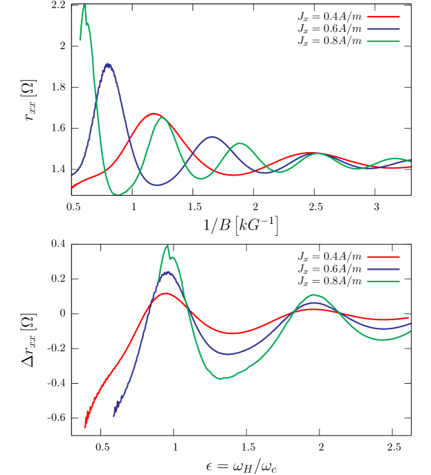
Figure 3: (color online) (a) Differential resistance $r_{xx}$ as a function $1/B$ and (b) Correction to the differential resistance $\Delta r_{xx}\,(\epsilon)$ for: $J_{x}=0.4A/m$ (red), $J_{x}=0.6A/m$ (blue) and $J_{x}=0.80A/m$ (green, higher peak).

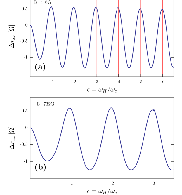
Figure 4: (color online) Correction to differential resistance $\Delta r_{xx}\,(\epsilon)$ obtained from $J_{x}$-sweeps at fixed values of $B=416G$ (a) and $B=712G$ (b).

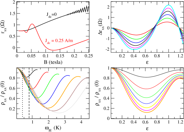
Figure 5: (color online) (a) Differential resistance $r_{xx}\,(B)$ for $J_{x}=0$ (black) and $J_{x}=0.25A/m$ (red). (b) Correction to differential resistance $\Delta r_{xx}\,(\epsilon)$ obtained varying $J_{x}$ at fixed values of $B$, from $B=0.5\,kG$ (red) to $B=1.75\,kG$ (light blue) in $0.25\,kG$ steps (top to botton at $\epsilon=0.4$). (c) Normalized longitudinal resistance as a function of $\omega_{H}$ for the same selection of values of the magnetic fields as in (b). The vertical line shows the value of $2\,\Gamma$, Eq. (15), for $B=0.5\,kG$ (dotted) and $B=1.75\,kG$ (dashed) showing good agreement with the half-width of the $J_{x}$ decay of $\rho_{xx}/\rho_{xx}(0)$. (d) This figure displays similar plots as a function of $\epsilon$.