The Seesaw Mechanism in Quark-Lepton Complementarity

Florian Plentinger, Gerhart Seidl, and Walter Winter

Institut für Theoretische Physik und Astrophysik, Universität Würzburg,

D-97074 Würzburg, Germany

Abstract

We systematically construct realistic mass matrices for the type-I seesaw mechanism out of more than 20 trillion possibilities. We use only very generic assumptions from extended quark-lepton complementarity, i.e., the leptonic mixing angles between flavor and mass eigenstates are either maximal, or parameterized by a single small quantity $\epsilon$ that is of the order of the Cabibbo angle $\epsilon\simeq\theta_{\text{C}}$. The small quantity $\epsilon$ also describes all fermion mass hierarchies. We show that special cases often considered in the literature, such as having a symmetric Dirac mass matrix or small mixing among charged leptons, constitute only a tiny fraction of our possibilities. Moreover, we find that in most cases the spectrum of right-handed neutrino masses is only mildly hierarchical. As a result, we provide for the charged leptons and neutrinos a selected list of $1\,981$ qualitatively different Yukawa coupling matrices (or textures) that are parameterized by the Cabibbo angle and allow for a perfect fit to current data. In addition, we also briefly show how the textures could be generated in explicit models from flavor symmetries.

1 Introduction

The impressive experimental advances that have been made during the past decade in solar [1, 2], atmospheric [3], reactor [4, 5], and accelerator [6] neutrino oscillation experiments, have very well established that neutrinos are massive. Since neutrinos are massless in the Standard Model (SM), the observation of neutrino masses provides evidence for new physics, such as an underlying Grand Unified Theory (GUT) [7] (see also Ref. [8]). It is therefore believed that the smallness of the absolute neutrino mass scale $m_{\nu}\simeq 10^{-2}\dots 10^{-1}\>\text{eV}$ compared to the electroweak scale $\sim 10^{2}\>\text{GeV}$ gives us important information on the nature of the new physics. Today, the most widely accepted mechanism to generate small neutrino masses is the seesaw mechanism [9, 10], in which the smallness of neutrino masses is linked to the hierarchy between the electroweak and the GUT scale $M_{\text{GUT}}\simeq 2\times 10^{16}\>\text{GeV}$ [11].

In the type-I seesaw mechanism [9], the set of SM neutrinos $\nu_{i}$ ($i=1,2,3$ is the generation index) is extended by three right-handed neutrinos $\nu_{i}^{c}$, which are total singlets under the SM gauge group $G_{\text{SM}}=SU(3)_{c}\times SU(2)_{L}\times U(1)_{Y}$. In the basis $(\nu_{1},\nu_{2},\nu_{3},\nu_{1}^{c},\nu_{2}^{c},\nu_{3}^{c})$, this leads after electroweak symmetry breaking to a complex symmetric $6\times 6$ matrix

$$M_{\nu}=\left(\begin{matrix}0&M_{D}\\ M_{D}^{T}&M_{R}\end{matrix}\right),$$ (1)

where 0, $M_{D}$, and $M_{R}$ are $3\times 3$ matrices. The upper left matrix 0 has zero entries since there is no Higgs triplet that could have directly coupled to the $\nu_{i}$. The entries in $M_{D}$ are protected by electroweak gauge invariance and they are therefore of the order $\sim 10^{2}\;\text{GeV}$, while the matrix elements of $M_{R}$ are of the order of the $B-L$ breaking scale $M_{B-L}\simeq 10^{14}\;\text{GeV}$. After integrating out the right-handed neutrinos, we arrive at the effective low-energy $3\times 3$ neutrino Majorana mass matrix

$$M_{\text{eff}}=-M_{D}M_{R}^{-1}M_{D}^{T},$$ (2)

which gives rise to neutrino masses of the order $m_{\nu}\simeq 10^{-2}\;\text{eV}$. The seesaw mechanism is attractive because $M_{B-L}$ is very close to $M_{\text{GUT}}$, indicating a GUT-origin of neutrino masses.

In GUT models, quarks and leptons are unified into multiplets, which is known as quark-lepton unification and one possibility to explore GUTs at present energies is to search for signatures of quark-lepton unification in the fermion mass and mixing parameters. Most notably, quark-lepton unification has to give an answer to the question why the quark mixing angles in the Cabibbo-Kobayashi-Maskawa (CKM) matrix $V_{\text{CKM}}$ [12] and the leptonic mixing angles in the Pontecorvo-Maki-Nakagawa-Sakata (PMNS) matrix $U_{\text{PMNS}}$ [13] are strikingly different. In the quark sector, all CKM mixing angles are small and can be approximately written as powers of the Cabibbo angle $\theta_{\text{C}}$. In contrast to this, in the lepton sector, only the reactor angle $\theta_{13}$ is small, whereas the solar angle $\theta_{12}$ and the atmospheric angle $\theta_{23}$ are both large. In addition, while the quark and charged lepton mass ratios are strongly hierarchical, the neutrino masses exhibit, if any, only a mild hierarchy (for a recent global fit of neutrino data see, e.g., Ref. [14]).

Recently, quark-lepton complementarity (QLC) [15] (for an early approach see Ref. [16]) has been proposed as a possibility to account for the differences between the quark and lepton mixings. In QLC, the quark and lepton mixing angles are connected by the QLC relations

$$\theta_{12}+\theta_{\text{C}}\approx\pi/4,\quad\theta_{23}+\theta_{cb}\approx\pi/4,$$ (3)

where $\theta_{cb}=\text{arcsin}\>V_{cb}$. The crucial observation is that sum rules of the types shown in Eq. (3) can be easily obtained when the mixing among the neutrinos and among the charged leptons is described by maximal or CKM-like mixing angles. In this way, for example, the observed value of the solar angle $\theta_{12}\approx 33^{\circ}$ could be understood in terms of maximal $(\pi/4)$ and Cabibbo-like ($\theta_{\text{C}}$) mixing in the individual neutrino and charged lepton sectors. A complementary approach to the solar angle seems, on the other hand, to be suggested by the tri-bimaximal mixing scheme [17]. The properties of QLC have been studied in various respects: as a result of deviations from bimaximal mixing [18], in connection with sum rules [19], with emphasis on phenomenological implications [20], together with parameterizations of $U_{\text{PMNS}}$ in terms of $\theta_{\text{C}}$ [21], in view of statistical arguments [22], in conjunction with renormalization group effects [23], and in model building realizations [24].

In Ref. [25], we have proposed an extended QLC, in which the mixing angles in both the charged lepton and the neutrino sector can take any value in the sequence $\pi/4,\epsilon,\epsilon^{2},\dots$, where $\epsilon$ is of the order the Cabibbo angle $\epsilon\simeq\theta_{\text{C}}$. In this paper, we will implement extended QLC in the type-I seesaw mechanism by assuming that all the mixing angles of charged leptons and left- and right-handed neutrinos take their values in this sequence. We also suggest that the mass eigenvalues of $M_{D}$ and $M_{R}$ are described by powers of $\epsilon$ as well. In this approach, the observed large mixing angles $\theta_{12}$ and $\theta_{23}$ can come from the charged leptons and/or neutrinos. Moreover, in the neutrino sector, large mixing angles can originate from $M_{D}$ and/or $M_{R}$. We systematically search for all mass matrices of charged leptons and neutrinos that satisfy the extended QLC assumptions, and extract all solutions that are consistent with current data in the CP conserving case.

The paper is organized as follows: We first motivate the assumptions underlying the extended QLC approach from the phenomenological and model building point of view in Sec. 2. This section can be skipped by the reader already familiar with extended QLC. Next, in Sec. 3, we describe the method for constructing all valid charged lepton and seesaw mass matrices that are compatible with data, demonstrate how to obtain the corresponding textures, and address further properties of our procedure. For the normal neutrino mass hierarchy, we first discuss the full sample of all valid mass matrices in Sec. 4, and then we show a selection of textures in Sec. 5. A qualitative discussion of the inverted and degenerate neutrino mass schemes is included in Sec. 6 and a summary and conclusions can be found in Sec. 7. Details of our method can be found in Appendix A and B.

2 Motivation

In this section, we first present a brief review of the observed hierarchies of fermion masses and mixing angles and relate them to a small expansion parameter $\epsilon$ that is of the order of the Cabibbo angle. Then, we discuss two representative $SU(5)$ GUT examples that obtain the observed mass and mixing parameters from flavor symmetries. The observations made here will later, in Sec. 3.2, serve as a motivation for the hypotheses in extended QLC.

2.1 Masses and Mixings of Quarks and Leptons

One of the most striking features of the fermion sector is that the mass and mixing parameters of quarks and charged leptons are strongly hierarchical. It is well known that these hierarchies can be approximately described by a small number $\epsilon\simeq 0.2$. In the Wolfenstein parameterization [28], for example, the CKM matrix is given by

$$V_{\text{CKM}}=\left(\begin{matrix}1-\frac{1}{2}\epsilon^{2}&\epsilon&A(\rho-{\text{i}}\eta)\epsilon^{3}\\ -\epsilon&1-\frac{1}{2}\epsilon^{2}&A\epsilon^{2}\\ A(1-\rho-\text{i}\eta)\epsilon^{3}&-A\epsilon^{2}&1\end{matrix}\right),$$ (4)

where $\epsilon$ is of the order of the Cabibbo angle $\theta_{\text{C}}\simeq 0.2$, and $A,\rho,$ and $\eta$, are order unity parameters (for an update see Ref. [29]). Order of magnitude wise, the quark mixing angles can be written in terms of the parameter $\epsilon$ as

$$|V_{us}|\sim\epsilon,\quad|V_{cb}|\sim\epsilon^{2},\quad|V_{ub}|\sim\epsilon^{3}.$$ (5)

An interesting connection between the Cabibbo angle and the quark masses is established by the Gatto-Sartori-Tonin-Oakes relation $\theta_{\text{C}}=\sqrt{m_{d}/m_{s}}$ [30], suggesting that also the fermion mass ratios arise from powers of $\epsilon$. In fact, the mass ratios of the up and down quarks can, e.g., be crudely represented as powers of $\epsilon$ as

$$m_{u}:m_{c}:m_{t}=\epsilon^{6}:\epsilon^{4}:1,\quad m_{d}:m_{s}:m_{b}=\epsilon^{4}:\epsilon^{2}:1,$$ (6)

where $m_{b}:m_{t}\sim\epsilon^{2}$, $m_{\tau}:m_{b}\sim 1$, and $m_{t}\simeq 175\>\text{GeV}$, whereas the mass ratios of the charged leptons are crudely given by

$$m_{e}:m_{\mu}:m_{\tau}=\epsilon^{4}:\epsilon^{2}:1.$$ (7)

These mass ratios have all to be understood as order of magnitude relations and depend on the energy scale. At one loop, in the minimal supersymmetric standard model (MSSM), the only changes in these relations are $m_{c}:m_{t}\sim\epsilon^{4}$ and $m_{b}:m_{t}\sim\epsilon^{3}$ at $\sim 10^{15}\;\text{GeV}$ (see, e.g., Ref. [31]). The changes due to renormalization group (RG) running are thus only comparatively small.

In the neutrino sector, we have a situation that is substantially different from the charged fermion sectors. Experimentally, the PMNS matrix reads (cf. also Ref. [32])

$$U_{\text{PMNS}}=\left(\begin{matrix}0.82-0.85&0.52-0.57&\leq 0.12\\ 0.26-0.49&0.48-0.68&0.65-0.76\\ 0.27-0.49&0.49-0.69&0.64-0.75\end{matrix}\right),$$ (8)

which has, unlike $V_{\text{CKM}}$, large off-diagonal entries. In the standard parameterization, the $1\sigma$ ranges for the solar and the atmospheric mixing angles are then [14]

$$\text{sin}^{2}\theta_{12}=0.30^{+0.02}_{-0.03},\quad\text{sin}^{2}\theta_{23}=0.5^{+0.08}_{-0.07},$$ (9)

whereas we have a $3\sigma$ upper bound on the reactor angle that is $\text{sin}^{2}\theta_{13}\leq 0.041$. The best fit values of the mixing angles correspond to maximal atmospheric mixing $\theta_{23}\approx\pi/4$ and large, but not maximal, solar mixing $\theta_{12}\approx\pi/4-\theta_{\text{C}}$, and a small reactor angle $\theta_{13}\lesssim\theta_{\text{C}}$. The $1\sigma$ bounds on the solar and atmospheric mass squared differences are [14]

$$\Delta m_{\odot}^{2}=(7.9^{+0.3}_{-0.3})\times 10^{-5}\text{eV}^{2},\quad\Delta m_{\text{atm}}^{2}=(2.5^{+0.2}_{-0.25})\times 10^{-3}\text{eV}^{2}.$$ (10)

The sign of $\Delta m_{\odot}^{2}$ is positive, whereas the sign of $\Delta m_{\text{atm}}^{2}$ can be either positive or negative, leading to currently three possible types of allowed neutrino mass spectra. Note that we roughly have

$$\Delta m_{\odot}^{2}:\Delta m_{\text{atm}}^{2}\sim\epsilon^{2}.$$ (11)

It is thus plausible that the neutrino sector, just like the quarks and charged leptons, is described by the same control parameter $\epsilon$. The order of magnitude relations for the neutrino masses may thus be written as

$$m_{1}:m_{2}:m_{3}=\epsilon^{2}:\epsilon:1,\quad m_{1}:m_{2}:m_{3}=1:1:\epsilon,\quad m_{1}:m_{2}:m_{3}=1:1:1,$$ (12)

where $m_{1},m_{2},$ and $m_{3}$, denote the masses of the 1st, 2nd, and 3rd neutrino mass eigenstate. The 1st, 2nd, and 3rd equation in Eq. (12) describe a normal hierarchical (NH), inverse hierarchical (IH), and quasi degenerate (QD) spectrum, respectively.

We thus see that the CKM angles and mass ratios of quarks and leptons are roughly given by some power $\sim\epsilon^{n}$ of the Cabibbo angle $\epsilon\simeq\theta_{\text{C}}$. Besides that, the phenomenological QLC relations $\theta_{23}\approx\pi/4-\epsilon^{2}$ and $\theta_{12}\approx\pi/4-\epsilon$ involve maximal mixing angles. In the next section, we will dicuss how these mass and mixing parameters may be reproduced in models.

2.2 Examples with Quark-Lepton Unification

The common appearance of the masses and mixing angles in the quark and lepton sectors may point towards a quark-lepton unified theory. One might therefore wonder whether a description of the fermion mass and mixing parameters as given in Sec. 2.1 can indeed be obtained in explicit models. We are interested in models in which the fermion mixing angles – prior to going to the mass eigenbasis – can be maximal or are given by some power of the Cabibbo angle $\epsilon\simeq\theta_{\text{C}}$ which also describes all fermion mass ratios.

For this purpose, let us briefly review two GUT models [33, 34] based on $SU(5)$, which show that in a quark-lepton unified theory it is (i) actually possible to generate realistic hierarchical fermion mass ratios and mixing angles that are described by powers $\sim\epsilon^{n}$ and that (ii) one can predict exact maximal mixing compatible with these hierarchies. We view the two GUT models as two representatives of a broad class of possible realistic models using Abelian (for early work see Ref. [35] and for more recent models see, e.g., Refs. [36, 31]) or discrete non-Abelian (for recent studies including the quark sector see, e.g., Ref. [37] and in the context of GUTs see, e.g., Ref. [38]) flavor symmetries. Our observations can be viewed as a further motivation for the definition of extended QLC in Sec. 3.2, where we will, in particular, claim that both the neutrinos as well as the charged leptons can exhibit mixing angles that are maximal and/or $\sim\epsilon^{n}$. In this way, the size of $\theta_{12}$ will then be simply the result of a QLC-type sum rule.

Example 1: Cabibbo-type mass and mixing hierarchies – Our first example is a supersymmetric $SU(5)^{\prime}\times SU(5)^{\prime\prime}$ GUT with a $U(1)^{N}=\Pi_{j=1}^{N}U(1)_{j}$ flavor symmetry group [33]. It yields, as a result of $U(1)^{N}$ flavor symmetry breaking, the masses and mixing angles of quarks and leptons roughly as powers of $\epsilon$. The $i$th generation $(i=1,2,3)$ is charged under $SU(5)^{\prime}\times U(1)_{k_{i}}$ ($k_{i}$ labels a suitable subgroup $U(1)_{k_{i}}\subset\Pi^{N}_{j=1}U(1)_{j}$) in an $SO(10)$ compatible way as ${\bf 10}(-1)_{i}+{\bf\overline{5}}(3)_{i}+{\bf 1}(-5)_{i}$, where the numbers in parenthesis denote the $U(1)_{k_{i}}$ charges of the respective multiplets and the $SU(5)$ singlets are the right-handed neutrinos. Higgs superfields break the $U(1)^{N}$ gauge symmetry such that masses for quarks and leptons arise from higher-dimension terms via the Froggatt-Nielsen mechanism [40] illustrated in Fig. 1.

Figure 1: Generation of higher-dimension fermion mass terms via the Froggatt-Nielsen mechanism. $\psi_{L}$ and $\psi_{R}$ are left- and right-handed SM fermions. Internal solid lines denote superheavy fermions with common mass $M_{F}$, the circled cross is the usual SM Higgs vacuum expectation value (VEV), whereas the crosses without circle represent universal VEVs $v$ of SM singlet scalars that break the flavor symmetry. After integrating out the heavy fermions, the resulting mass term is then given by the effective dimension-$n$ operator $\langle H\rangle\epsilon^{n}\overline{\psi}_{L}\psi_{R}$, where $\epsilon=v/M_{F}$ serves as a small expansion parameter.

In the presence of SM singlet scalar “flavons”, that break the flavor symmetry by acquiring universal vacuum expectation values (VEVs) $v$ (crosses), and superheavy fermions with common mass $M_{F}$, which are charged under the flavor symmetry (internal solid lines), the mass terms of quarks and leptons become suppressed by integer powers of a small parameter $\epsilon=v/M_{F}$ that controls the flavor symmetry breaking. The integer power of $\epsilon$ is solely determined by the quantum numbers of the left- and right-handed fermions $\psi_{L}$ and $\psi_{R}$ under the flavor symmetry. As a result, the mass matrices of the up quarks, down quarks, charged leptons, and neutrinos become

$$M_{u}=m_{t}\left(\begin{matrix}\epsilon^{6}&\epsilon^{5}&\epsilon^{3}\\ \epsilon^{5}&\epsilon^{4}&\epsilon^{2}\\ \epsilon^{3}&\epsilon^{2}&1\end{matrix}\right),\quad M_{d}=M_{\ell}^{T}=m_{b}\left(\begin{matrix}\epsilon^{4}&\epsilon^{6}&\epsilon^{3}\\ \epsilon^{10}&\epsilon^{2}&\epsilon^{2}\\ \epsilon^{8}&\epsilon^{3}&1\end{matrix}\right),\quad M_{\text{eff}}=m_{\nu}\left(\begin{matrix}\epsilon^{4}&\epsilon^{2}&\epsilon\\ \epsilon^{2}&1&1\\ \epsilon&1&1\end{matrix}\right).$$ (13)

The representation of the mass matrices in Eq. (13) are examples of what we will call in the following textures: These are descriptions of the mass matrices showing only the order of magnitude (up to order one Yukawa couplings) of the entries in terms of powers of a small number $\epsilon$ that parameterizes the flavor symmetry breaking. At an order of magnitude level, the textures in Eqs. (13) predict for the quarks and charged leptons the mass ratios and mixing angles of Eqs. (5), (6), and (7), whereas the neutrino mass spectrum is of the type $m_{1}:m_{2}:m_{3}=\epsilon:\epsilon:1$. The reactor mixing angle is small and of the order $\theta_{13}\sim\epsilon$, while the solar and the atmospheric mixing angles are large and of the orders $\theta_{12}\sim 1$ and $\theta_{23}\sim 1$. A proper choice of the order one Yukawa couplings then allows to reproduce the solar and atmospheric mixing angles close to the current best fit values.

Example 2: Maximal mixing – Our second example is an $SU(5)$ GUT with a non-Abelian discrete flavor symmetry between the 2nd and 3rd generation [34]. It predicts a maximal atmospheric mixing angle $\theta_{23}=\pi/4$ and a zero reactor angle $\theta_{13}=0$ as a consequence of the discrete symmetry. The basic flavor symmetry of the model is a discrete $Z_{2}$ exchange symmetry that implements a maximal atmospheric mixing angle and acts on the $SU(5)$ multiplets of the 2nd and 3rd generation as $Z_{2}:\,{\bf\overline{5}}_{2}\leftrightarrow{\bf\overline{5}}_{3},\>{\bf 10}_{2}\leftrightarrow{\bf 10}_{3},\>{\bf 1}_{2}\leftrightarrow{\bf 1}_{3},$ where the subscripts denote the generation indices. In addition, the model has a $U(1)$ family number symmetry that does not commute with the above $Z_{2}$ generator. As a consequence, the resulting down quark and charged lepton mass matrices can accommodate the hierarchical down quark and charged lepton masses and the CKM and PMNS mixing angles arise in the up quark and the neutrino sector, respectively. The total non-Abelian flavor symmetry enforces in $M_{\text{eff}}$ a $\mu-\tau$ exchange symmetry. This predicts a maximal atmospheric mixing angle $\theta_{23}=\frac{\pi}{4}$ and a vanishing reactor angle $\theta_{13}=0$. The solar angle $\theta_{12}$, on the other hand, is large and can easily reproduce the current best fit value.

These two examples show that hierarchical masses and mixings described by powers of $\epsilon$ as well as maximal mixing can be predicted in explicit GUT models from flavor symmetries. As a result of this motivation section, it is therefore plausible to assume that all mixing angles and mass hierarchies in the quark and lepton sectors are generated by a single small quantity $\epsilon\simeq\theta_{\text{C}}$ augmented by possibly maximal mixing in the up- and/or down-type sectors. This basic observation will be the basis for our hypotheses underlying extended QLC.

3 Method

In this section, we introduce our method for implementing extended QLC in the seesaw mechanism. For this purpose, we first briefly review the seesaw mechanism and discuss our notation for parameterizing the mass and mixing parameters in Sec. 3.1. Next, we define our QLC assumptions in Sec. 3.2, and outline our approach for generating and selecting the mass matrices of charged leptons and neutrinos in Sec. 3.3, i.e., we describe our general procedure. While Sec. 3.3 is somewhat qualitative in some points, we give more details and a comment on the complexity in Appendix A. As the next step, we demonstrate how we produce textures in Sec. 3.4. Finally, we discuss the role of mass ratios, input parameters, and RG running in our routine in Sec. 3.5.

3.1 Neutrino Mass and Mixing Nomenclature

In what follows, we assume that the left-handed SM neutrinos acquire their masses via the type-I seesaw mechanism [9]. In the type-I seesaw mechanism, the Yukawa couplings generating the charged lepton and neutrino masses are

$$\mathcal{L}_{\text{Y}}=-(Y_{\ell})_{ij}H^{\ast}\ell_{i}e^{c}_{j}-(Y_{D})_{ij}\text{i}\sigma^{2}H\ell_{i}\nu_{j}^{c}-\frac{1}{2}(M_{R})_{ij}\nu^{c}_{i}\nu^{c}_{j}+\text{h.c.},$$ (14a)

where $$\ell_{i}=(\nu_{i},\>e_{i})^{T} e_{i}^{c} \nu^{c}_{i} i=1,2,3 \ell_{i} e^{c}_{i} \nu_{i}^{c} H Y_{\ell} Y_{D} 3\times 3 Y_{\ell} Y_{D} M_{R} 3\times 3 \text{i}\sigma^{2} 2\times 2 H \langle H\rangle=(0,v/\sqrt{2})^{T} v\sim 10^{2}\>\text{GeV}$$, , and ( is the generation index), are the left-handed lepton doublets (), the right-handed charged leptons (), and the right-handed SM singlet neutrinos (). In Eq. (14a), is the Higgs doublet, and are the Dirac Yukawa coupling matrices of the charged leptons () and neutrinos (), is the Majorana mass matrix of the right-handed neutrinos, and is the antisymmetric tensor. After electroweak symmetry breaking, develops a vacuum expectation value , where , and the mass terms of the leptons become

$$\mathcal{L}_{\text{mass}}=-(M_{\ell})_{ij}e_{i}e^{c}_{j}-(M_{D})_{ij}\nu_{i}\nu_{j}^{c}-\frac{1}{2}(M_{R})_{ij}\nu^{c}_{i}\nu^{c}_{j}+\text{h.c.},$$ (14b)

where $M_{\ell}=\langle H\rangle Y_{\ell}$ is the charged lepton and $M_{D}=\langle H\rangle Y_{D}$ the Dirac neutrino mass matrix. $M_{\ell}$ and $M_{D}$ are complex $3\times 3$ matrices that are described by 18 parameters and have entries of the order $\sim 10^{2}\>\text{GeV}$. The matrix $M_{R}$ is complex, symmetric, and described by 12 parameters. It has matrix elements of the order the $B-L$ breaking scale $M_{B-L}\sim 10^{15}\>\text{GeV}$. The resulting complex symmetric $6\times 6$ neutrino mass matrix is given in Eq. (1), and after integrating out the right-handed neutrinos, this gives the effective $3\times 3$ neutrino mass matrix $M_{\text{eff}}$ in Eq. (2) leading to masses $\sim 10^{-2}\;\text{eV}$ for the active neutrinos.

To analyze the origin of leptonic mixing, we consider the diagonalization of the mass terms in $\mathcal{L}_{\text{mass}}$ in Eq. (14b) by unitary matrices. Using the convention in Ref. [25], we can always write a general unitary $3\times 3$ matrix $U_{\text{unitary}}$ as

$$U_{\text{unitary}}=\text{diag}\left(e^{\text{i}\varphi_{1}},e^{\text{i}\varphi_{2}},e^{\text{i}\varphi_{3}}\right)\cdot\widehat{U}\cdot\text{diag}\left(e^{\text{i}\alpha_{1}},e^{\text{i}\alpha_{2}},1\right),$$ (15a)

where the phases $$\varphi_{1} \varphi_{2} \varphi_{3} \alpha_{1} \alpha_{2} \left[0,2\pi\right]$$, , , , and , take their values in the interval and

$$\widehat{U}=\left(\begin{array}[]{ccc}c_{12}c_{13}&s_{12}c_{13}&s_{13}e^{-\text{i}\widehat{\delta}}\\ -s_{12}c_{23}-c_{12}s_{23}s_{13}e^{\text{i}\widehat{\delta}}&c_{12}c_{23}-s_{12}s_{23}s_{13}e^{\text{i}\widehat{\delta}}&s_{23}c_{13}\\ s_{12}s_{23}-c_{12}c_{23}s_{13}e^{\text{i}\widehat{\delta}}&-c_{12}s_{23}-s_{12}c_{23}s_{13}e^{\text{i}\widehat{\delta}}&c_{23}c_{13}\end{array}\right)$$ (15b)

is a CKM-like matrix in the standard parameterization with $s_{ij}=\sin\hat{\theta}_{ij}$, $c_{ij}=\cos\hat{\theta}_{ij}$, where $\hat{\theta}_{ij}\in\{\hat{\theta}_{12},\hat{\theta}_{13},\hat{\theta}_{23}\}$ lie all in the first quadrant, i.e., $\hat{\theta}_{ij}\in\left[0,\frac{\pi}{2}\right]$, and $\widehat{\delta}\in[0,2\pi]$. The matrix $\widehat{U}$ is thus described by 3 mixing angles $\theta_{ij}$ and one phase $\delta$, i.e., it has 4 parameters. The matrix $U_{\text{unitary}}$ has five additional phases and contains therefore in total 9 parameters.

The leptonic Dirac mass matrices $M_{\ell}$ and $M_{D}$, and the Majorana mass matrices $M_{R}$ and $M_{\text{eff}}$ are diagonalized by

$$M_{\ell}=U_{\ell}M_{\ell}^{\text{diag}}U_{\ell^{\prime}}^{\dagger},\quad M_{D}=U_{D}M_{D}^{\text{diag}}U_{D^{\prime}}^{\dagger},\quad M_{R}=U_{R}M_{R}^{\text{diag}}U_{R}^{T},\quad M_{\text{eff}}=U_{\nu}M_{\text{eff}}^{\text{diag}}U_{\nu}^{T},$$ (16)

where $U_{\ell},U_{\ell^{\prime}},U_{D},U_{D^{\prime}},U_{R}$, and $U_{\nu}$, are unitary mixing matrices, whereas $M_{\ell}^{\text{diag}},M_{D}^{\text{diag}},M_{R}^{\text{diag}},$ and $M_{\text{eff}}^{\text{diag}}$, are diagonal mass matrices with positive entries. We can always write the mixing matrices as the products

$$U_{x}=D_{x}\widehat{U}_{x}K_{x},$$ (17)

where $\widehat{U}_{x}$ are CKM-like matrices that are parameterized as in Eq. (15b), while $D_{x}$ and $K_{x}$ are given by $D_{x}=\text{diag}(e^{\text{i}\varphi_{1}^{x}},e^{\text{i}\varphi_{2}^{x}},e^{\text{i}\varphi_{3}^{x}})$ and $K_{x}=\text{diag}(e^{\text{i}\alpha_{1}^{x}},e^{\text{i}\alpha_{2}^{x}},1)$, where the index $x$ runs over $x=\ell,\ell^{\prime},D,D^{\prime},R,\nu$. The phases in $D_{x}$ and $K_{x}$ are all in the range $\varphi_{1}^{x},\varphi_{2}^{x},\varphi_{3}^{x},\alpha_{1}^{x},\alpha_{2}^{x}\in[0,2\pi]$. Each of the matrices $\widehat{U}_{x}$ in Eq. (17) contains four mixing parameters: three mixing angles and one phase. We denote the parameters of $\widehat{U}_{x}$ by $\theta_{12}^{x},\theta_{13}^{x},\theta_{23}^{x},$ and $\delta^{x}$. For each of the matrices $\widehat{U}_{x}$ in Eq. (17), we define the mixing parameters by identifying in Eq. (15b) the mixing angles as $\hat{\theta}_{ij}\rightarrow\theta_{ij}^{x}$, and the phase as $\widehat{\delta}\rightarrow\delta^{x}$.

The PMNS matrix is given by

$$U_{\text{PMNS}}=U_{\ell}^{\dagger}U_{\nu}=\widehat{U}_{\text{PMNS}}K_{\text{Maj}},$$ (18)

where $\widehat{U}$ is a CKM-like matrix parameterized as in Eq. (15b), and $K_{\text{Maj}}=\text{diag}(e^{\text{i}\phi_{1}},e^{\text{i}\phi_{2}},1)$ contains the Majorana phases $\phi_{1}$ and $\phi_{2}$. The CKM-like matrix $\widehat{U}_{\text{PMNS}}$ in Eq. (18) is described by the solar angle $\theta_{12}$, the reactor angle $\theta_{13}$, the atmospheric angle $\theta_{23}$, and the Dirac CP-phase $\delta$, which we identify in the standard parameterization of Eq. (15b) as $\hat{\theta}_{ij}\rightarrow\theta_{ij}$ and $\widehat{\delta}\rightarrow\delta$. The PMNS matrix has thus 3 mixing angles and 3 phases and contains therefore 6 physical parameters.

Let us next express $M_{\text{eff}}$ in terms of the mass eigenvalues and mixing angles introduced above. Inserting Eq. (17) into Eq. (16), we find

$$M_{D} = D_{D}\widehat{U}_{D}K_{D}M_{D}^{\mathrm{diag}}K_{D^{\prime}}^{*}\widehat{U}_{D^{\prime}}^{\dagger}D_{D^{\prime}}^{*}\,,$$ (19a)

$$M_{R}^{-1} = D_{R}^{*}\widehat{U}_{R}^{\ast}K_{R}^{*}(M_{R}^{\mathrm{diag}})^{-1}K_{R}^{*}\widehat{U}_{R}^{\dagger}D_{R}^{*}~{}.$$ (19b)

The effective neutrino mass matrix $M_{\text{eff}}$ in Eq. (2) can thus be written as

$$M^{\text{th}}_{\text{eff}}=-D_{D}\widehat{U}_{D}\tilde{K}M_{D}^{\mathrm{diag}}\widehat{U}_{D^{\prime}}^{\dagger}\tilde{D}\widehat{U}_{R}^{*}(K_{R}^{*})^{2}(M_{R}^{\mathrm{diag}})^{-1}\widehat{U}_{R}^{\dagger}\tilde{D}\widehat{U}_{D^{\prime}}^{*}M_{D}^{\mathrm{diag}}\tilde{K}\widehat{U}_{D}^{T}D_{D}~{},$$ (20a)

where we have introduced $$\tilde{K}=K_{D}^{\ast}K_{D^{\prime}} \tilde{D}=D_{D^{\prime}}^{\ast}D_{R}^{\ast} M_{\text{eff}} (K_{R}^{\ast})^{2} M_{\text{eff}} M_{\text{eff}} M_{\text{eff}}$$ and . We have denoted the parameterization of in Eq. (20a) by an extra superscript “th” for “theoretical”, since none of the mass and mixing parameters on the right-hand side of Eq. (20a) are directly measurable in neutrino oscillations. Note that in the CP conserving case, the matrix drops out of the expression for in Eq. (20a). Equivalently to Eq. (20a), using Eqs. (18) and (17) in the expression for in Eq. (16), we can write also in the parameterization

$$M_{\text{eff}}^{\text{exp}}=D_{\ell}\widehat{U}_{\ell}K_{\ell}\widehat{U}_{\text{PMNS}}K^{2}_{\text{Maj}}M^{\text{diag}}_{\text{eff}}\widehat{U}^{T}_{\text{PMNS}}K_{\ell}\widehat{U}_{\ell}^{T}D_{\ell}~{},$$ (20b)

where we have chosen the superscript “exp” for “experimental”, to label the representation of $M_{\text{eff}}$ in Eq. (20b), since $M_{\text{eff}}^{\text{exp}}$ involves the matrices $M_{\text{eff}}^{\text{diag}}$ and $U_{\text{PMNS}}$ containing the experimentally accessible mass and mixing parameters. Note that in the CP conserving case, $(K_{\text{Maj}})^{2}$ drops out of the expression for $M_{\text{eff}}^{\text{exp}}$. It is clear that $M_{\text{eff}}^{\text{th}}=M_{\text{eff}}^{\text{exp}}=M_{\text{eff}}$, since $M_{\text{eff}}^{\text{th}}$ and $M_{\text{eff}}^{\text{exp}}$ are just different parameterizations of $M_{\text{eff}}$.

3.2 Hypotheses for Extended QLC

We will now formulate the assumptions underlying extended QLC in the type-I seesaw mechanism. Motivated by the discussion of the GUT examples in Sec. 2.2, extended QLC will in this context include assumptions on (i) the mixing parameters of $U_{\ell},U_{D},U_{D^{\prime}},$ and $U_{R}$, and assumptions on (ii) the eigenvalues of the mass matrices $M_{\ell},M_{\text{eff}},M_{D},$ and $M_{R}$.

Mixing angles – Consider first the possible mixing angles in extended QLC. Following the idea of Ref. [25], we begin by assuming that all mixing angles parameterizing in Eq. (16) the mixing matrices $U_{\ell},U_{D},U_{D^{\prime}}$, and $U_{R}$, can a priori take any of the values in the sequence $\pi/4,\epsilon,\epsilon^{2},\dots$, where $\epsilon$ is a small number. Motivated by the quark sector, we will take $\epsilon\simeq 0.2$, i.e., we assume that $\epsilon$ is of the order the Cabibbo angle. This applies the concept of extended quark-lepton complementarity in Ref. [25] to the mixing matrices $U_{D}$, $U_{D^{\prime}},$ and $U_{R}$, that diagonalize the renormalizable neutrino mass terms in Eq. (14b). Since the current $1\sigma$ error on the leptonic mixing angles is at most of the order $\epsilon^{2}$ (see, e.g., Ref. [14]), we will truncate the sequence of mixing angles $\pi/4,\epsilon,\epsilon^{2},\dots$ after the element $\epsilon^{2}$ and identify there all terms of the order $\epsilon^{n}$ with $n\geq 3$ simply by “$0$”. In other words, in extended QLC, we restrict the possible range of mixing angles $\theta_{ij}^{x}$ ($x=\ell,D,D^{\prime},R$) to the set of values $\theta_{ij}^{x}\in\{\pi/4,\epsilon,\epsilon^{2},0\}$, where “$0$” represents mixing angles $\sim\epsilon^{n}$ with $n\geq 3$. Since we want to compare with current neutrino data, the assumptions on the mixing angles are formulated at low energies $\sim 1\;\text{GeV}$. The impact of RG running when assuming these angles at a high scale will be discussed later in Sec. 3.5. Note that we cannot just rotate away $U_{\ell}$, because this would make our mixing angle assumptions as powers of $\epsilon$ meaningless if induced by an underlying theory, such as a flavor symmetry.

Mass eigenvalues – Next, let us specify the types of mass eigenvalues that we assume in extended QLC. We have to distinguish two types of mass eigenvalues – those of the lepton mass matrices $M_{\ell}$ and $M_{\text{eff}}$ in the low-energy effective theory, and those of the Dirac and heavy Majorana mass matrices $M_{D}$ and $M_{R}$ of the neutrinos.

We assume that the mass spectra in the low energy effective theory are those of Eq. (7) and Eq. (12). That means we assume $m_{e}:m_{\mu}:m_{\tau}=\epsilon^{4}:\epsilon^{2}:1$ for the charged leptons, whereas we have in the neutrino sector $m_{1}:m_{2}:m_{3}=\epsilon^{2}:\epsilon:1$ for a NH, $m_{1}:m_{2}:m_{3}=1:1:\epsilon$ for an IH, and $m_{1}:m_{2}:m_{3}=1:1:1$ for a QD neutrino mass spectrum. As we will discuss later, our results are actually completely independent from the details of the charged lepton spectrum.

Let us now consider the mass eigenvalues of the Dirac and Majorana mass matrices $M_{D}$ and $M_{R}$. We denote the mass eigenvalues of $M_{D}$ by $m_{1}^{D},m_{2}^{D},$ and $m_{3}^{D}$, and the mass eigenvalues of $M_{R}$ by $m_{1}^{R},m_{2}^{R},$ and $m_{3}^{R}$. Notice that these are not directly observable at low energies, but as before, we write the mass eigenvalues of $M_{D}$ and $M_{R}$ as powers of $\epsilon$. Similar to Eqs. (7) and (12), we will therefore parameterize the mass eigenvalues $M_{D}$ and $M_{R}$ as

$$m_{1}^{D}:m_{2}^{D}:m_{3}^{D}=\epsilon^{a}:\epsilon^{b}:\epsilon^{c}\quad\text{and}\quad m_{1}^{R}:m_{2}^{R}:m_{3}^{R}=\epsilon^{a^{\prime}}:\epsilon^{b^{\prime}}:\epsilon^{c^{\prime}},$$ (21)

where $a,b,c,a^{\prime},b^{\prime},$ and $c^{\prime}$, are suitable non-negative integers $\leq 2$, and we define the absolute mass scales by $m_{3}^{D}=m_{D}\epsilon^{c}$ and $m_{3}^{R}=M_{B-L}\epsilon^{c^{\prime}}$. As we will discuss in Appendix A.1, one can restrict the possible range of the integers in Eq. (21) to a fairly small set of numbers, such that it is sufficient to test all possible combinations up to second order in $\epsilon$.

In total, we see that in our hypotheses for extended QLC all mass hierarchies and small mixing angles become described by powers of the hierarchy parameter $\epsilon$. In Sec. 3.5, we will discuss the validity and precision of our assumptions in extended QLC when taking, e.g., GUT relations among fermion masses and RG effects into account.

3.3 Procedure: Systematic Construction of the Parameter Space

Figure 2: Procedure for obtaining the seesaw realizations and texture sets in extended QLC.

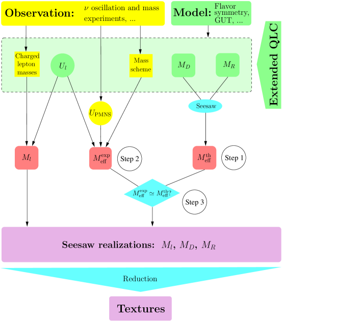
Let us now describe our three-step procedure for generating all textures $M_{\ell}$, $M_{D}$, and $M_{R}$, which satisfy extended QLC for the seesaw mechanism (cf., Fig. 2 for illustration):

First step – We generate all possibilities for the effective neutrino mass matrix $M^{\text{th}}_{\text{eff}}$ in Eq. (20a). Here, we assume that the mixing angles entering $U_{D},U_{D^{\prime}},$ and $U_{R}$, can take any values in the set

$$\theta_{ij}^{x}\in\{\pi/4,\epsilon,\epsilon^{2},0\},$$ (22)

where $x=D,D^{\prime},R$. Moreover, we suppose in Eq. (20a) that $M^{\text{diag}}_{D}$ and $M^{\text{diag}}_{R}$ are on the general forms as given in Eq. (21) with eigenvalues $1,\epsilon$ or$\epsilon^{2}$. For simplicity, we will confine ourselves to the CP conserving case were all phases are taken from the set $\delta^{x},\varphi_{1}^{x},\varphi_{2}^{x},\varphi_{3}^{x},\alpha_{1}^{x},\alpha_{2}^{x}\in\{0,\pi\}$.

Second step – We generate all possibilities for the neutrino mass matrix $M^{\text{exp}}_{\text{eff}}$ in Eq. (20b). For $U_{\text{PMNS}}$, we use values motivated by the current best-fit values. In particular, we use the following input, which could be experimentally confirmed or rejected in the coming years

$$\theta_{12}=\pi/4-\epsilon,\quad\theta_{13}=0,\quad\theta_{23}=\pi/4\,$$ (23)

with $\epsilon=0.2$. These values represent the current best-fit values [14] very closely. A different choice for these parameters can be equally well applied, but it will change the final results.

For $U_{\ell}$, we follow Eq. (22), and for the phases, we test all real possibilities. Furthermore, we insert the neutrino mass spectra given in Eq. (12) into $M_{\text{eff}}^{\text{diag}}$, and again test all possibilities.

Third step – Next, we match all possibilities from step 1 and step 2, i.e., we select all parameter combinations for which

$$M_{\text{eff}}^{\text{th}}|_{\epsilon=0.2}\simeq M_{\text{eff}}^{\text{exp}}|_{\epsilon=0.2}\,$$ (24)

at $\mathcal{O}(\epsilon^{3})$. For details (and the exact numerical implementation) of the matching procedure, see Appendix A.2; in particular, note that our procedure automatically factors out the overall neutrino mass scale, i.e., $m_{\nu}=m_{D}^{2}/M_{R}$ will be automatically satisfied. In the following, we will call a (seesaw) realization a valid set $\{M_{D},M_{R},U_{\ell}\}$, or more precisely, a combination of all involved mixing parameters, phases, and mass hierarchies, for which Eq. (24) is fulfilled. In other words, a realization is thus a set of input parameters compatible with current experimental best-fit values which describes $M_{\text{eff}}^{\text{th}}$ and the $6\times 6$ matrix $M_{\nu}$ completely, and it contains the left-handed charged lepton mixing. In total, our procedure requires that we systematically scan 20 trillion different possible realizations. For details on the complexity, see Appendix A.3.

Note that in our procedure the observed large leptonic mixing angles can be generated either in the charged lepton sector and/or the neutrino sector. Furthermore, in the neutrino sector, large mixings can arise from the Dirac neutrino and/or the Majorana mass matrix of the right-handed neutrinos. This means that we not make any special assumptions simplifying the structure of the seesaw mechanism, such as taking $M_{\ell}$ or $M_{R}$ to be diagonal, or $M_{D}$ symmetric.

3.4 Texture Extraction and Order Unity Couplings

Let us now describe how we extract the textures for the charged leptons and neutrinos from the seesaw realizations that satisfy Eq. (24). In the course of applying the three step procedure described in Sec. 3.3, we have already produced for each realization the pair of matrices $M_{D}$ and $M_{R}$. In the same way, we determine for each valid realization the charged lepton mass matrix $M_{\ell}$ by rotating to the left-handed flavor basis as $M_{\ell}=U_{\ell}M_{\ell}^{\text{diag}}$, where $M_{\ell}^{\text{diag}}$ contains the masses given in Eq. (7). Next, we analytically expand the mass matrices in $\epsilon$ as

$$M_{x}=M_{x}^{(0)}+M_{x}^{(1)}\epsilon+M_{x}^{(2)}\epsilon^{2}+\mathcal{O}(\epsilon^{3}),$$ (25)

where $x=\ell,D,R,$ and identify for each matrix element the leading contribution as the lowest order in $\epsilon$. The texture for $M_{x}$ is then found by substituting each matrix element of $M_{x}$ by its leading power $\epsilon^{k}$. For $k\geq 3$, we take $\epsilon^{k}\rightarrow 0$. In doing so, we always “drop” the order one coefficients that multiply the leading powers $\epsilon^{k}$ and round them to one (unless they are zero). For a given realization, we call the collection of textures for $M_{\ell},M_{D},$ and $M_{R}$ a texture set. For any texture set obtained in this way, we argue that one can always adjust the order unity coefficients such that the Yukawa couplings are brought in perfect agreement with data. An important prerequisite for this statement is that the different orders in the expansion in Eq. (25) do not “interfere” with each other, i.e., the involved coefficients are really of order unity. This property for the coefficients will be checked below. It is important to keep in mind that, in general, more than one realization may lead to the same texture set. Because of the reduction from in general several realizations to one texture set, we will call our texture set producing technique “texture reduction”. Note also the important fact that the texture reduction is based on an analytic expansion in $\epsilon$ as opposed to just using powers of $0.2$ for a purely numerical fit of the mass matrix elements.

As an example for texture reduction, consider the following mass matrix $M_{D}$ (cf., texture/realization #1 in Table LABEL:tab:seesawtextures):

$$M_{D}=m_{D}\,\left(\begin{array}[]{ccc}-\frac{\epsilon^{2}}{\sqrt{2}}&-\epsilon&0\\ -\epsilon^{2}&-\frac{1}{\sqrt{2}}+\frac{\epsilon^{2}}{2\sqrt{2}}&\frac{1}{\sqrt{2}}-\frac{\epsilon^{2}}{2\sqrt{2}}\\ \frac{\epsilon^{2}}{\sqrt{2}}&-\frac{\epsilon^{2}}{\sqrt{2}}&-\epsilon+\frac{\epsilon^{2}}{\sqrt{2}}\end{array}\right)\longrightarrow\left(\begin{array}[]{ccc}\epsilon^{2}&\epsilon&0\\ \epsilon^{2}&1&1\\ \epsilon^{2}&\epsilon^{2}&\epsilon\end{array}\right).$$

Here, “$\rightarrow$” symbolizes, up to an overall mass scale, the identification of the leading order terms in the expansion in $\epsilon$ that contribute to the mass matrix elements in $M_{D}$. The matrix on the right hand side of $\rightarrow$ then represents the texture corresponding to the mass matrix $M_{D}$ on the left hand side.

Figure 3: Distribution of the order one couplings in $M_{\ell}$ (left), $M_{D}$ (center) and $M_{R}$ (right) for all valid seesaw realizations of NH neutrinos (of all orders and for all matrix elements). The gray-shaded region marks the area in which the order one couplings are smaller than $\epsilon$.

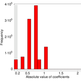
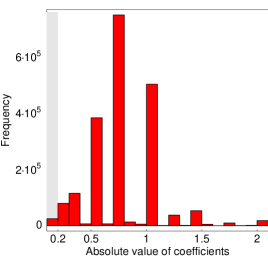
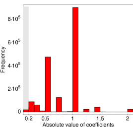
In order for the expansion in Eq. (25) to be useful, the Yukawa couplings should be of order unity (at least if one wants not to rely on some sort of fine-tuning). The expansion suggests a criterion for what “order unity” actually means: the coefficients should lie in the interval $[\epsilon,\dots,\epsilon^{-1}]\simeq[0.2,\dots,5]$, such that they would not imitate different orders in $\epsilon$. In Fig. 3, we show to which extent this condition is indeed satisfied for the valid realizations. Fig. 3 depicts the coefficients of the $M_{x}^{(i)}$ in Eq. (25) for $M_{\ell}$ (left), $M_{D}$ (center) and $M_{R}$ (right) for all valid seesaw realizations and NH neutrinos (including all orders and for all matrix elements). Interestingly, it turns out that in 99.9% of all cases, the order unity Yukawa couplings lie in the range $\epsilon,\dots,\epsilon^{-1}$, which justifies the expansion of the textures in $\epsilon$. For example, for $M_{\ell}$ and $M_{D}$, the peaks at around $0.7\simeq 1/\sqrt{2}$ are predominant. Note that, though in Fig. 3 the first bin corresponds to coefficients smaller than $\epsilon$, our mapping of textures is unambiguous. This is because in the cases where the leading order coefficient of a matrix element becomes very small ($<0.2$), the other coefficients become also very small – with the exception of $0.10\%$ of all cases for the matrix elements. As a consequence, the leading order term indeed rarely numerically interferes with the higher orders. This picture would change if $\epsilon$ was larger. For instance, for $\epsilon=0.5$, the leading order identification for $M_{D}$ fails in $0.43\%$ of all cases, and for $M_{R}$ it fails in $0.01\%$ of all cases, which is, however, still only a remarkably small fraction of all cases.

3.5 Dependence on Input and Renormalization Group Effects

Let us now discuss how the choice of the input parameters from measurement affects our results. First of all, we use the current best-fit values as an input (cf., Eq. (23)). Any other choice of experimental input parameters will give different results, but our procedure can be equally well applied to any other preferred choice of input values. We have chosen these input values because these results can be expected to remain valid for the next ten years or so, unless the best-fit values change (such as if $\sin^{2}2\theta_{13}\sim 0.1$ were indeed found). We have also computed the dataset for different values of $\theta_{13}$, but a presentation of these results would clearly exceed the scope of this paper.

As far as the charged lepton mass spectra in Eq. (7) are concerned, a variation of the mass ratios will not have any effect at all on the selection and extraction of the texture sets: Any change in the spectrum drops completely out of our routine. The particular choice of the charged lepton mass hierarchies in Eq. (7) has been motivated by comparison with the down quark spectrum in $SU(5)$. Choosing a different parameterization of the charged lepton masses, for example with different powers of $\epsilon$, will of course have an effect on the form of the extracted texture sets for $M_{\ell}$, but it does not affect the selection of the realizations in any way. In particular, a modification of the charged lepton mass spectra in Eq. (7), e.g., to implement the Georgi-Jarlskog relation $m_{\mu}:m_{\tau}=3\,m_{s}:m_{b}$ [48], would not change any of our results for the textures. In fact, one can easily obtain the textures of the charged leptons for any other choice of the hierarchy by using $U_{\ell}$ directly.

The extended QLC hypotheses in Sec. 3.2 should hold at high energies such as $M_{\text{GUT}}$, but they are compared in our method with low-energy data. We therefore have to address the stability of the extended QLC assumptions under RG running from the high scale down to, say, around $\sim 1\,\text{GeV}$. Generally, the empirical QLC sum rule $\theta_{12}=\pi/4-\theta_{\text{C}}$ is satisfied up to a precision of about $\sim 1^{\circ}$. It is therefore reasonable to take in our routine nonzero mixing angles $\theta^{x}_{ij}$ into account that can be as small as $\epsilon^{2}\sim 2^{\circ}$. Moreover, it is known that the Cabibbo angle $\theta_{\text{C}}$ does practically not run [49], and $V_{cb}\sim\epsilon^{2}$ changes typically only by a factor smaller than 2 when running from $\sim 1\,\text{GeV}$ up to the Planck scale $\sim 10^{19}\,\text{GeV}$ [50].

Let us have a more precise look at the RG evolution of neutrino masses and mixings [51]. First, note that, due to the smallness of the charged lepton Yukawa couplings, the running of a possibly maximal atmospheric mixing angle $\theta_{23}$ is negligible, unless one works in the MSSM with large $\text{tan}\,\beta$ [43]. Simple expressions for the running of lepton mixing angles have been recently presented in Ref. [52]: When running $M_{\text{eff}}$ from the GUT scale down to low energies, the corrections to the leptonic mixing angle $\theta_{ij}$ are smaller than $\sim|m_{i}+m_{j}|^{2}(|m_{i}|^{2}-|m_{j}|^{2})^{-1}\times 10^{-2}$, where $m_{i}$ and $m_{j}$ are the eigenvalues of the $i$th and $j$th neutrino mass eigenstates of $M_{\text{eff}}$ at the GUT scale. An appreciable running of leptonic mixing angles can thus only be expected in the IH or QD case. For NH neutrinos, however, the corrections are $\lesssim 1^{\circ}$ and, thus, negligible. Moreover, a tuning of phases always allows to switch off completely any RG effect on neutrino mixing angles – even in the case of inverse hierarchical and degenerate neutrinos [52]. A similar result has been obtained in the bottom-up approach in Ref. [53], where the starting point are the fixed low-energy observables. In addition, while the overall neutrino mass scale is affected by RG running, the neutrino mass ratios are hardly changed. Since our results should be very stable under RG running for the NH case (irrespective of the phases), we will focus in this paper on this type of hierarchy.

4 Currently Allowed Realizations for the NH Case

In this section, we focus on the constructed set of currently allowed seesaw realizations for a normal neutrino mass hierarchy (NH case). We obtain $173\,084$ different realizations for the NH case, which reduce to $8\,030$ cases if one does not count different phase combinations as different cases. This leads to $1\,981$ different texture sets, i.e., different combinations of $M_{\ell}$, $M_{D}$, and $M_{R}$. Naturally, we cannot show all of these possibilities in this paper. In Sec. 5, we will therfore apply some selection criteria to reduce this dataset further and present the texture sets which seem to be most interesting to us. In this section, however, we discuss general features and some statistics of the constructed seesaw realizations for NH neutrinos.

We concentrate on NH also because RG effects on neutrino mass ratios and mixing angles are expected to be small in this case (see Sec. 3.5). This means that our generic assumptions, which may hold at some high energy scale (say at $\sim 10^{16}\;\text{GeV}$), do not change significantly when running down to low energies where we match to experiment. In the NH case, one can easily diagonalize $M_{\text{eff}}$ for the allowed realizations in order to check that Eq. (24) produces observables in agreement with current data. We have done this exercise: We have determined $U_{\nu}$ by diagonalizing $M_{\text{eff}}$ and computed $U_{\mathrm{PMNS}}=U_{\ell}^{\dagger}U_{\nu}$ employing the corresponding matrix $U_{\ell}$. From $U_{\mathrm{PMNS}}$, one can read off the mixing angles just as described in Ref. [25]. Note that we do not expect to reproduce exactly our input values in Eq. (23), since we do not require exact matching precision in Eq. (24) (see also Appendix A.2).

Figure 4: Distribution of valid seesaw realizations for the NH case as a function of $\chi^{2}$ as defined in Eq. (26). The values of $\theta_{13}$ are all in agreement with current data.

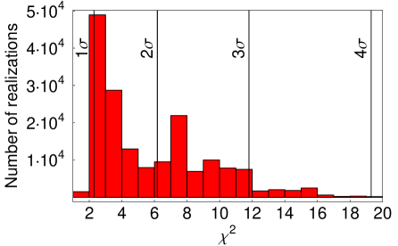
To describe the compatibility of a realization with current data, we use the performance indicator

$$\chi^{2}\equiv\left(\frac{\sin^{2}\theta_{12}-0.3}{0.3\times\sigma_{12}}\right)^{2}+\left(\frac{\sin^{2}\theta_{23}-0.5}{0.5\times\sigma_{23}}\right)^{2}~{},$$ (26)

(e.g., $\chi^{2}=11.83$ corresponds to a $3\sigma$ CL exclusion for 2 d.o.f.). This corresponds to a Gaussian $\chi^{2}$ approximation in $\sin^{2}\theta_{12}$ and $\sin^{2}\theta_{23}$ with the current best-fit values. For the relative $1\sigma$ errors, we use $\sigma_{12}\simeq 9\%$ (for $\sin^{2}\theta_{12}$) and $\sigma_{23}\simeq 16\%$ (for $\sin^{2}\theta_{23}$) [14]. Note that we only find $\sin^{2}\theta_{13}\ll 0.04$ below the current bound, i.e., we do not have to impose an additional selection criterion. Fig. 4 shows the distribution of the valid seesaw realizations as a function of $\chi^{2}$ defined in Eq. (26). Obviously, Eq. (24) already ensures that the neutrino mixing angles of each realization are compatible with current bounds. It turns out that in all valid cases $\theta_{13}\ll 1^{\circ}$ and only 6.5% of the realizations lead to $11.83\lesssim\chi^{2}\lesssim 17$ (which corresponds to a CL between $3$ and $4\sigma$ for 2 d.o.f.). Therefore, the selected realizations are all in perfect agreement with current data. Note that one might naively expect to find realizations with $\theta_{13}$ around the best-fit value of $0^{\circ}$ since this value has been used as an input for $M_{\text{eff}}^{\text{exp}}$. However, in almost all cases one obtains $\theta_{23}$ to be around $50^{\circ}$ despite of the best-fit input value of $45^{\circ}$.

Figure 5: Distributions of hierarchies in $M_{D}$ (left) and $M_{R}$ (right) leading to a NH neutrino masses for all valid seesaw realizations.

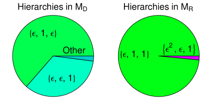
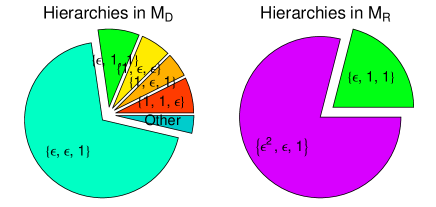
Fig. 5, shows the distribution of mass spectra or hierarchies proportional to $(m_{1}^{D},m_{2}^{D},m_{3}^{D})$ and $(m_{1}^{R},m_{2}^{R},m_{3}^{R})$ for $M_{D}$ and $M_{R}$ respectively (each normalized to the corresponding heaviest mass eigenvalue of $M_{D}$ and $M_{R}$) for the NH case. These distributions are obtained by simply counting the number of realizations with a certain mass spectrum. Observe that $M_{R}$ has as a mass spectrum only $(\epsilon^{2},\epsilon,1)$ and $(\epsilon,1,1)$. Note that the spectra labeled as $(\epsilon^{2},\epsilon,1)$ include also strongly hierarchical cases where the right-handed Majorana neutrino mass spectrum can actually be $(\epsilon^{n},\epsilon,1)$, with some suitable $n\geq 3$ (see Appendix A.1). Fig. 5 shows that, for $M_{R}$, in all valid seesaw realizations, the mildly hierarchical mass spectrum $(\epsilon,1,1)$ clearly dominates the (strongly) the hierarchical spectrum $(\epsilon^{n},\epsilon,1)$ with $n\geq 2$. As it will turn out later in Sec. 5, this observation is also supported at the texture-level: more than 80% of the extracted textures lead to a mild mass hierarchy $(\epsilon,1,1)$ for the right-handed neutrino masses. We will come back to this point in the next paragraph. The absence of a degenerate mass spectrum for $M_{R}$ in the NH (and IH) case is a simple consequence and selection effect of Eq. (27c) in combination with the assumption $M_{\text{eff}}^{\text{exp}}\sim\text{diag}(\epsilon^{2},\epsilon,1)$. There are many more possibilities for the mass spectra of $M_{D}$ but they are dominated by the types $(\epsilon,1,\epsilon)$ and $(\epsilon,\epsilon,1)$. In Fig. 5, the pie piece “Other” also contains the hierarchy $(\epsilon^{2},\epsilon,1)$, which implies that we have the same hierarchy in $M_{R}$ (but not vice versa). In our method, no charged-lepton or quark-type hierarchy is produced. We find from Fig. 5 that there are many possibilities to obtain a normal neutrino mass hierarchy, but one cannot claim that this hierarchy appears typically in $M_{D}$ or $M_{R}$ and then translates into $M_{\text{eff}}$.

The distributions of mass spectra in Fig. 5 may have immediate relevance for leptogenesis [55] when crudely extrapolating our results to the CP non-conserving case. In at least 80% of the cases that we found (cf., Sec. 5), the right-handed neutrino mass spectrum is of the mildly hierarchical form $(\epsilon,1,1)$. Thus, if the mass $m_{1}^{R}$ of the lightest right-handed neutrino is in the range $m_{1}^{R}\lesssim 10^{12}\>\text{GeV}$, the seesaw scale set by the mass of the heaviest right-handed neutrino $m_{3}^{R}$ would have to be significantly lower than the usual $B-L$ breaking scale $\sim 10^{14}\>\text{GeV}$. For the mildly hierarchical right-handed neutrino mass spectrum $(\epsilon,1,1)$, successful leptogenesis might be achieved in two ways: (i) via resonant leptogenesis [56] (for recent models see, e.g., Ref. [57]) or (ii) by taking flavor effects into account [58] (for a connection with low-energy CP-violation see, e.g., Ref. [59]). In the resonant limit, $m_{3}^{R}$ could be as low as several TeV, thereby making this scenario testable at a collider. Strongly hierarchical right-handed neutrino masses, which is the standard case considered in the literature for leptogenesis, are in our analysis found to be by about a factor of 5 less abundant than the mild hierarchy. The possible strongly hierarchical right-handed neutrino mass spectra are all of the type $(\epsilon^{n},\epsilon,1)$, where $n\geq 2$. Allowing $n$ to be sufficiently large (say $n=8$), the strongly hierarchical case can fit into a scheme with a seesaw scale of the order $m_{3}^{R}\sim 10^{14}\>\text{GeV}$ and sufficient baryon asymmetry could again be generated through flavored leptogenesis.

Figure 6: Distributions of mixings in $U_{D}$, $U_{D^{\prime}}$, $U_{R}$, and $U_{\ell}$ (in columns) leading to a normal neutrino mass hierarchy. The different pie labels refer to the number of maximal mixing angles, where “All small” corresponds to all mixing angles $\leq\epsilon$.

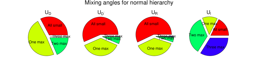
Fig. 6 shows the distributions of mixing angles, where we concentrate on the number of maximal (“max”) mixing angles $\theta_{ij}^{x}=\pi/4$ appearing in $U_{D}$, $U_{D^{\prime}}$, $U_{R}$, and $U_{\ell}$. If there is no maximal mixing angle, we call the scenario “All small“. Let us first note that the distributions of the mixing angles in $M_{\nu}$ are very different from $U_{\ell}$. In $U_{\ell}$, we often find large mixings, which means that the large lepton mixing angles are not necessarily created in the neutrino sector, but can also come very often from the charged lepton sector. Note that the pie slice “All small” in $U_{\ell}$ represents more or less CKM-like mixings in $U_{\ell}$. There are also many possibilities with “trimaximal” mixing (i.e., all three mixing angles $\theta_{ij}^{x}$ are maximal for some given sector $x$) in $U_{\ell}$. This is different from the other mixing matrices, where trimaximal mixing hardly occurs, and either one maximal mixing angle or only small mixing angles are preferred. In particular, in $U_{D^{\prime}}$ and $U_{R}$, only small mixings are typical.

Figure 7: Fraction of special cases for normal mass hierarchy. The different pies show the fractions of the cases with symmetric $M_{D}$, diagonal $M_{R}$, and $U_{\ell}\simeq\mathbbm{1}$, of all allowed realizations (not texture sets). This figure is based on the mixing matrices, where $U_{D}\simeq U_{D^{\prime}}$ in the first case, $U_{R}\simeq\mathbbm{1}$ and $U_{\ell}\simeq\mathbbm{1}$ in the second and third case, respectively. For the similarity condition “$\simeq$”, we allow $\epsilon^{2}$-deviations in the mixing angles. For instance, for an exact $U_{R}=\mathbbm{1}$, one would have only 2% of all realizations.

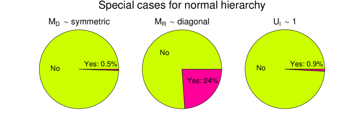
Fig. 7 shows the fraction of realizations that exhibit symmetric $M_{D}$, and/or diagonal $M_{R}$, and/or $U_{\ell}\simeq\mathbbm{1}$. In this figure, “$M_{D}\sim$ symmetric” means that $M_{D}$ is symmetric up to possible corrections of the order $\epsilon^{2}$. It is evident that there are only very few realizations with symmetric $M_{D}$ or $U_{\ell}\simeq\mathbbm{1}$, and none with diagonal $M_{D}$, which is not surprising from what we have learned above. One may conclude from this result that there are plenty of possibilities to implement the seesaw mechanism without these constraints, which have, however, often been imposed in existing literature.

Generally, note that, while one may argue that one can construct more possibilities in a more general and sophisticated framework, our realizations result from very generic and simple assumptions without adding another level of complexity. In this sense, our generic assumptions are much simpler than ad-hoc constraints, such as requiring that $U_{\ell}$ be diagonal. It is interesting to note that we find for $M_{R}$ quite many realizations that are close to a diagonal form.

5 A Selection of Textures for the NH Case

In this section, we present a selection of texture sets for the NH case. These texture sets satisfy certain selection criteria listed in App. B.1. The full set of the texture sets is available in Ref. [60]. Table LABEL:tab:seesawtextures shows these 72 texture sets for $M_{\ell},M_{D},$ and $M_{R}$, together with associated example realizations leading to these texture sets. For each texture set, we always choose the realization with the lowest $\chi^{2}$, i.e., the realization which fits data best. For this realization, the table lists the mass spectra of $M_{D}$ and $M_{R}$, as well as the mixing angles $\theta^{x}_{ij}$ in the different sectors. For each case in Table LABEL:tab:seesawtextures, we have collected in Table LABEL:tab:seesawtexturesphases (in App. B.2) all the corresponding phases ($0$ or $\pi$) in order to allowing for a complete reconstruction of the realizations and Yukawa coupling matrices. In addition, one can find there the PMNS mixing angles, as well as the number of realizations that become identified with each texture set through the texture reduction. In Table LABEL:tab:seesawtextures, the parameter $\xi$ can take the values $\xi\in\{0,\epsilon^{2}\}$.

Table 1: Complete set of selected seesaw textures/realizations for the NH case, where $\xi\in\{0,\epsilon^{2}\}$ (see text).

#	$M_{\ell}$	$M_{D}$	$M_{R}$	$\begin{array}[]{@{\hspace{0.5mm}}c@{\hspace{0.5mm}}}\hskip 1.42262pt\lx@intercol\hfil m_{i}^{D}/m_{D}\hfil\hskip 1.42262pt\\[2.84526pt] \hskip 1.42262pt\lx@intercol\hfil m_{i}^{R}/M_{B-L}\hfil\hskip 1.42262pt\end{array}$	$\begin{array}[]{@{\hspace{0.5mm}}c@{\hspace{0.5mm}}}\hskip 1.42262pt\lx@intercol\hfil(\theta_{12}^{\ell},\theta_{13}^{\ell},\theta_{23}^{\ell})\hfil\hskip 1.42262pt\\[2.84526pt] \hskip 1.42262pt\lx@intercol\hfil(\theta_{12}^{D},\theta_{13}^{D},\theta_{23}^{D})\hfil\hskip 1.42262pt\\[2.84526pt] \hskip 1.42262pt\lx@intercol\hfil(\theta_{12}^{D^{\prime}},\theta_{13}^{D^{\prime}},\theta_{23}^{D^{\prime}})\hfil\hskip 1.42262pt\\[2.84526pt] \hskip 1.42262pt\lx@intercol\hfil(\theta_{12}^{R},\theta_{13}^{R},\theta_{23}^{R})\hfil\hskip 1.42262pt\end{array}$
$1$	$\left(\begin{array}[]{ccc}0&0&\epsilon\\ 0&\epsilon^{2}&1\\ 0&\epsilon^{2}&1\end{array}\right)$	$\left(\begin{array}[]{ccc}\epsilon^{2}&\epsilon&0\\ \xi&1&1\\ \epsilon^{2}&\xi&\epsilon\end{array}\right)$	$\left(\begin{array}[]{ccc}\epsilon^{2}&0&0\\ 0&1&1\\ 0&1&1\end{array}\right)$	$\begin{array}[]{c}(\epsilon^{2},1,\epsilon)\vspace{0.1cm}\\ (\epsilon^{2},\epsilon,1)\end{array}$	$\begin{array}[]{c}(\xi,\epsilon,\frac{\pi}{4})\\ (\epsilon,\frac{\pi}{4},\xi)\\ (\xi,\xi,\frac{\pi}{4})\\ (\xi,0,\frac{\pi}{4})\end{array}$
$2$	$\left(\begin{array}[]{ccc}0&0&1\\ 0&\epsilon^{2}&\epsilon\\ 0&0&1\end{array}\right)$	$\left(\begin{array}[]{ccc}\epsilon&1&\epsilon\\ \epsilon&1&\epsilon^{2}\\ \epsilon&1&\epsilon\end{array}\right)$	$\left(\begin{array}[]{ccc}1&\epsilon&1\\ \epsilon&1&\epsilon\\ 1&\epsilon&1\end{array}\right)$	$\begin{array}[]{c}(\epsilon,1,\epsilon)\vspace{0.1cm}\\ (\epsilon,1,1)\end{array}$	$\begin{array}[]{c}(\epsilon,\frac{\pi}{4},\epsilon)\\ (\frac{\pi}{4},\frac{\pi}{4},\epsilon^{2})\\ (\epsilon^{2},\epsilon,0)\\ (\epsilon^{2},\frac{\pi}{4},\epsilon)\end{array}$
$3$	$\left(\begin{array}[]{ccc}0&\epsilon^{2}&1\\ 0&\epsilon^{2}&1\\ 0&\epsilon^{2}&1\end{array}\right)$	$\left(\begin{array}[]{ccc}\epsilon&\epsilon^{2}&\epsilon\\ \epsilon^{2}&1&\epsilon\\ \epsilon&\epsilon&\epsilon\end{array}\right)$	$\left(\begin{array}[]{ccc}1&\epsilon&1\\ \epsilon&1&\epsilon\\ 1&\epsilon&1\end{array}\right)$	$\begin{array}[]{c}(\epsilon,1,\epsilon)\vspace{0.1cm}\\ (\epsilon,1,1)\end{array}$	$\begin{array}[]{c}(\frac{\pi}{4},\frac{\pi}{4},\frac{\pi}{4})\\ (0,\frac{\pi}{4},\epsilon)\\ (\epsilon^{2},\epsilon^{2},\epsilon)\\ (\epsilon,\frac{\pi}{4},\epsilon^{2})\end{array}$
$4$	$\left(\begin{array}[]{ccc}0&0&\epsilon\\ 0&\epsilon^{2}&1\\ 0&\epsilon^{2}&1\end{array}\right)$	$\left(\begin{array}[]{ccc}\epsilon&\epsilon&\epsilon\\ \epsilon&\epsilon&\epsilon\\ \xi&1&1\end{array}\right)$	$\left(\begin{array}[]{ccc}\epsilon&\epsilon&\epsilon\\ \epsilon&1&\epsilon^{2}\\ \epsilon&\epsilon^{2}&1\end{array}\right)$	$\begin{array}[]{c}(\epsilon,\epsilon,1)\vspace{0.1cm}\\ (\epsilon,1,1)\end{array}$	$\begin{array}[]{c}(\epsilon,\epsilon,\frac{\pi}{4})\\ (\frac{\pi}{4},\xi,\xi)\\ (\epsilon,\xi,\frac{\pi}{4})\\ (\epsilon,\epsilon,\xi)\end{array}$
$5$	$\left(\begin{array}[]{ccc}0&0&\epsilon\\ 0&\epsilon^{2}&1\\ 0&\epsilon^{2}&1\end{array}\right)$	$\left(\begin{array}[]{ccc}0&\epsilon&\epsilon\\ 1&1&1\\ 0&\epsilon&\epsilon\end{array}\right)$	$\left(\begin{array}[]{ccc}1&\epsilon&1\\ \epsilon&1&\epsilon\\ 1&\epsilon&1\end{array}\right)$	$\begin{array}[]{c}(\epsilon,1,\epsilon)\vspace{0.1cm}\\ (\epsilon,1,1)\end{array}$	$\begin{array}[]{c}(0,\epsilon,\frac{\pi}{4})\\ (\epsilon,\frac{\pi}{4},0)\\ (\frac{\pi}{4},\epsilon^{2},\frac{\pi}{4})\\ (\epsilon,\frac{\pi}{4},\epsilon^{2})\end{array}$
$6$	$\left(\begin{array}[]{ccc}0&0&\xi\\ 0&\epsilon^{2}&1\\ 0&\epsilon^{2}&1\end{array}\right)$	$\left(\begin{array}[]{ccc}\epsilon&\epsilon&\epsilon\\ \epsilon&1&\epsilon^{2}\\ \epsilon&\epsilon&\epsilon\end{array}\right)$	$\left(\begin{array}[]{ccc}\epsilon&\epsilon&\epsilon\\ \epsilon&1&\epsilon^{2}\\ \epsilon&\epsilon^{2}&1\end{array}\right)$	$\begin{array}[]{c}(\epsilon,1,\epsilon)\vspace{0.1cm}\\ (\epsilon,1,1)\end{array}$	$\begin{array}[]{c}(\epsilon,\xi,\frac{\pi}{4})\\ (\epsilon,\frac{\pi}{4},\epsilon)\\ (\epsilon,\epsilon,\xi)\\ (\epsilon,\epsilon,\epsilon)\end{array}$
$7$	$\left(\begin{array}[]{ccc}0&0&\xi\\ 0&\epsilon^{2}&1\\ 0&\epsilon^{2}&1\end{array}\right)$	$\left(\begin{array}[]{ccc}\epsilon&\epsilon&\epsilon\\ \epsilon&1&\epsilon\\ \epsilon&\epsilon&\epsilon\end{array}\right)$	$\left(\begin{array}[]{ccc}\epsilon&\epsilon&\epsilon\\ \epsilon&1&\epsilon^{2}\\ \epsilon&\epsilon^{2}&1\end{array}\right)$	$\begin{array}[]{c}(\epsilon,1,\epsilon)\vspace{0.1cm}\\ (\epsilon,1,1)\end{array}$	$\begin{array}[]{c}(\epsilon,\xi,\frac{\pi}{4})\\ (\epsilon,\frac{\pi}{4},\epsilon)\\ (\epsilon,\epsilon,\epsilon)\\ (\epsilon,\epsilon,\xi)\end{array}$
$8$	$\left(\begin{array}[]{ccc}0&0&\epsilon\\ 0&\epsilon^{2}&1\\ 0&\epsilon^{2}&1\end{array}\right)$	$\left(\begin{array}[]{ccc}\epsilon&\epsilon&\xi\\ \epsilon&\epsilon&\xi\\ \xi&\xi&1\end{array}\right)$	$\left(\begin{array}[]{ccc}\epsilon&\epsilon&0\\ \epsilon&1&0\\ 0&0&1\end{array}\right)$	$\begin{array}[]{c}(\epsilon,\epsilon,1)\vspace{0.1cm}\\ (\epsilon,1,1)\end{array}$	$\begin{array}[]{c}(\epsilon,\epsilon,\frac{\pi}{4})\\ (\frac{\pi}{4},\xi,\xi)\\ (\epsilon,\xi,\xi)\\ (\epsilon,\epsilon,\frac{\pi}{4})\end{array}$
$9$	$\left(\begin{array}[]{ccc}0&\epsilon^{2}&\epsilon\\ 0&\epsilon^{2}&1\\ 0&\epsilon^{2}&1\end{array}\right)$	$\left(\begin{array}[]{ccc}1&1&1\\ \epsilon^{2}&\epsilon&\epsilon\\ 1&1&1\end{array}\right)$	$\left(\begin{array}[]{ccc}1&\xi&1\\ \xi&1&\xi\\ 1&\xi&1\end{array}\right)$	$\begin{array}[]{c}(1,\epsilon,\epsilon)\vspace{0.1cm}\\ (\epsilon,1,1)\end{array}$	$\begin{array}[]{c}(\frac{\pi}{4},\epsilon,\frac{\pi}{4})\\ (\xi,\frac{\pi}{4},\xi)\\ (\epsilon,\frac{\pi}{4},\frac{\pi}{4})\\ (\xi,\frac{\pi}{4},\xi)\end{array}$
$10$	$\left(\begin{array}[]{ccc}0&0&\xi\\ 0&\epsilon^{2}&1\\ 0&\epsilon^{2}&1\end{array}\right)$	$\left(\begin{array}[]{ccc}\epsilon&\epsilon&\epsilon\\ \epsilon^{2}&1&\epsilon\\ \epsilon&\epsilon&\epsilon\end{array}\right)$	$\left(\begin{array}[]{ccc}\epsilon&0&\xi\\ 0&1&0\\ \xi&0&1\end{array}\right)$	$\begin{array}[]{c}(\epsilon,1,\epsilon)\vspace{0.1cm}\\ (\epsilon,1,1)\end{array}$	$\begin{array}[]{c}(\epsilon,\xi,\frac{\pi}{4})\\ (\epsilon,\frac{\pi}{4},\xi)\\ (0,0,\epsilon)\\ (0,\xi,\xi)\end{array}$
$11$	$\left(\begin{array}[]{ccc}0&0&\xi\\ 0&\epsilon^{2}&1\\ 0&\epsilon^{2}&1\end{array}\right)$	$\left(\begin{array}[]{ccc}\epsilon&\epsilon&\epsilon\\ \epsilon^{2}&1&\xi\\ \epsilon&\epsilon&\epsilon\end{array}\right)$	$\left(\begin{array}[]{ccc}\epsilon&0&\xi\\ 0&1&0\\ \xi&0&1\end{array}\right)$	$\begin{array}[]{c}(\epsilon,1,\epsilon)\vspace{0.1cm}\\ (\epsilon,1,1)\end{array}$	$\begin{array}[]{c}(\epsilon,\xi,\frac{\pi}{4})\\ (\epsilon,\frac{\pi}{4},\xi)\\ (0,0,\xi)\\ (0,\xi,\epsilon)\end{array}$
$12$	$\left(\begin{array}[]{ccc}0&\epsilon^{2}&1\\ 0&\epsilon^{2}&1\\ 0&\epsilon^{2}&1\end{array}\right)$	$\left(\begin{array}[]{ccc}\epsilon&0&\xi\\ 0&\epsilon&\epsilon\\ \xi&\epsilon&1\end{array}\right)$	$\left(\begin{array}[]{ccc}\epsilon&\xi&\xi\\ \xi&1&0\\ \xi&0&1\end{array}\right)$	$\begin{array}[]{c}(\epsilon,\epsilon,1)\vspace{0.1cm}\\ (\epsilon,1,1)\end{array}$	$\begin{array}[]{c}(\frac{\pi}{4},\frac{\pi}{4},\frac{\pi}{4})\\ (\xi,\xi,\epsilon)\\ (\xi,\xi,\epsilon)\\ (\xi,\xi,\epsilon)\end{array}$
$13$	$\left(\begin{array}[]{ccc}0&0&\epsilon\\ 0&\epsilon^{2}&1\\ 0&\epsilon^{2}&1\end{array}\right)$	$\left(\begin{array}[]{c@{\hspace{2mm}}cc}\epsilon\hfil\hskip 5.69054pt&\epsilon&\epsilon\\ \epsilon^{2}-\xi\hfil\hskip 5.69054pt&1&\xi\\ \epsilon\hfil\hskip 5.69054pt&\epsilon&\epsilon\end{array}\right)$	$\left(\begin{array}[]{ccc}\epsilon&0&\epsilon\\ 0&1&0\\ \epsilon&0&1\end{array}\right)$	$\begin{array}[]{c}(\epsilon,1,\epsilon)\vspace{0.1cm}\\ (\epsilon,1,1)\end{array}$	$\begin{array}[]{c}(\xi,\epsilon,\frac{\pi}{4})\\ (\epsilon,\frac{\pi}{4},\xi)\\ (\xi,\xi,\xi)\\ (\epsilon,\epsilon,\frac{\pi}{4})\end{array}$
$14$	$\left(\begin{array}[]{ccc}0&\epsilon^{2}&1\\ 0&\epsilon^{2}&1\\ 0&\epsilon^{2}&1\end{array}\right)$	$\left(\begin{array}[]{cc@{\hspace{2mm}}c}\epsilon&\epsilon^{2}\hfil\hskip 5.69054pt&\epsilon^{2}\\ \epsilon&1\hfil\hskip 5.69054pt&\epsilon^{2}-\xi\\ \epsilon^{2}&\epsilon\hfil\hskip 5.69054pt&\epsilon\end{array}\right)$	$\left(\begin{array}[]{ccc}\epsilon&\epsilon&\epsilon\\ \epsilon&1&\epsilon^{2}\\ \epsilon&\epsilon^{2}&1\end{array}\right)$	$\begin{array}[]{c}(\epsilon,1,\epsilon)\vspace{0.1cm}\\ (\epsilon,1,1)\end{array}$	$\begin{array}[]{c}(\frac{\pi}{4},\frac{\pi}{4},\frac{\pi}{4})\\ (\xi,\epsilon,\epsilon)\\ (\epsilon,\xi,\xi)\\ (\epsilon,\epsilon,\xi)\end{array}$
$15$	$\left(\begin{array}[]{ccc}0&\epsilon^{2}&1\\ 0&\epsilon^{2}&1\\ 0&\epsilon^{2}&1\end{array}\right)$	$\left(\begin{array}[]{ccc}\epsilon&0&\epsilon\\ \epsilon^{2}&1&\epsilon^{2}\\ \epsilon&\epsilon&\epsilon\end{array}\right)$	$\left(\begin{array}[]{ccc}1&\epsilon&1\\ \epsilon&1&\epsilon\\ 1&\epsilon&1\end{array}\right)$	$\begin{array}[]{c}(\epsilon,1,\epsilon)\vspace{0.1cm}\\ (\epsilon,1,1)\end{array}$	$\begin{array}[]{c}(\frac{\pi}{4},\frac{\pi}{4},\frac{\pi}{4})\\ (0,\frac{\pi}{4},\epsilon)\\ (\epsilon^{2},\epsilon^{2},\epsilon^{2})\\ (\epsilon,\frac{\pi}{4},\epsilon)\end{array}$
$16$	$\left(\begin{array}[]{ccc}0&\epsilon^{2}&1\\ 0&\epsilon^{2}&1\\ 0&\epsilon^{2}&1\end{array}\right)$	$\left(\begin{array}[]{ccc}\epsilon&\epsilon&\epsilon^{2}\\ 1&1&\epsilon^{2}\\ \epsilon&\epsilon&\epsilon\end{array}\right)$	$\left(\begin{array}[]{ccc}1&1&\epsilon\\ 1&1&\epsilon\\ \epsilon&\epsilon&1\end{array}\right)$	$\begin{array}[]{c}(\epsilon,1,\epsilon)\vspace{0.1cm}\\ (\epsilon,1,1)\end{array}$	$\begin{array}[]{c}(\frac{\pi}{4},\frac{\pi}{4},\frac{\pi}{4})\\ (\epsilon^{2},\epsilon,\epsilon)\\ (\frac{\pi}{4},\epsilon^{2},0)\\ (\frac{\pi}{4},\epsilon,\epsilon^{2})\end{array}$
$17$	$\left(\begin{array}[]{ccc}0&\epsilon^{2}&1\\ 0&\epsilon^{2}&\epsilon\\ 0&\epsilon^{2}&1\end{array}\right)$	$\left(\begin{array}[]{ccc}\epsilon&\epsilon^{2}&\epsilon\\ 1&\epsilon&1\\ 1&\epsilon&1\end{array}\right)$	$\left(\begin{array}[]{ccc}1&\epsilon&1\\ \epsilon&1&\epsilon\\ 1&\epsilon&1\end{array}\right)$	$\begin{array}[]{c}(\epsilon,\epsilon,1)\vspace{0.1cm}\\ (\epsilon,1,1)\end{array}$	$\begin{array}[]{c}(\frac{\pi}{4},\frac{\pi}{4},\epsilon)\\ (\epsilon,\epsilon^{2},\frac{\pi}{4})\\ (0,\frac{\pi}{4},\epsilon^{2})\\ (\epsilon,\frac{\pi}{4},\epsilon^{2})\end{array}$
$18$	$\left(\begin{array}[]{ccc}0&\epsilon^{2}&1\\ 0&\epsilon^{2}&1\\ 0&\epsilon^{2}&1\end{array}\right)$	$\left(\begin{array}[]{ccc}\epsilon&\epsilon&0\\ \epsilon&\epsilon&\epsilon\\ \epsilon^{2}&\epsilon^{2}&1\end{array}\right)$	$\left(\begin{array}[]{ccc}1&1&0\\ 1&1&0\\ 0&0&1\end{array}\right)$	$\begin{array}[]{c}(\epsilon,\epsilon,1)\vspace{0.1cm}\\ (\epsilon,1,1)\end{array}$	$\begin{array}[]{c}(\frac{\pi}{4},\frac{\pi}{4},\frac{\pi}{4})\\ (\frac{\pi}{4},0,\epsilon)\\ (\epsilon^{2},\epsilon^{2},\epsilon^{2})\\ (\frac{\pi}{4},\epsilon,\epsilon)\end{array}$
$19$	$\left(\begin{array}[]{ccc}0&\epsilon^{2}&1\\ 0&\epsilon^{2}&1\\ 0&\epsilon^{2}&1\end{array}\right)$	$\left(\begin{array}[]{ccc}\epsilon&\epsilon^{2}&\epsilon\\ \epsilon&\epsilon&\epsilon\\ 1&\epsilon&1\end{array}\right)$	$\left(\begin{array}[]{ccc}1&0&1\\ 0&1&0\\ 1&0&1\end{array}\right)$	$\begin{array}[]{c}(\epsilon,\epsilon,1)\vspace{0.1cm}\\ (\epsilon,1,1)\end{array}$	$\begin{array}[]{c}(\frac{\pi}{4},\frac{\pi}{4},\frac{\pi}{4})\\ (\epsilon,\epsilon^{2},\epsilon)\\ (0,\frac{\pi}{4},\epsilon)\\ (0,\frac{\pi}{4},0)\end{array}$
$20$	$\left(\begin{array}[]{ccc}0&0&\epsilon\\ 0&\epsilon^{2}&\xi\\ 0&0&1\end{array}\right)$	$\left(\begin{array}[]{ccc}\epsilon&\epsilon&\epsilon\\ \epsilon&1&1\\ \epsilon&1&1\end{array}\right)$	$\left(\begin{array}[]{ccc}\epsilon&\epsilon&\epsilon\\ \epsilon&1&\epsilon^{2}\\ \epsilon&\epsilon^{2}&1\end{array}\right)$	$\begin{array}[]{c}(\epsilon,1,\epsilon)\vspace{0.1cm}\\ (\epsilon,1,1)\end{array}$	$\begin{array}[]{c}(\xi,\epsilon,\xi)\\ (\epsilon,\epsilon,\frac{\pi}{4})\\ (0,\frac{\pi}{4},\frac{\pi}{4})\\ (\epsilon,\epsilon,\epsilon)\end{array}$
$21$	$\left(\begin{array}[]{ccc}0&\epsilon^{2}&1\\ 0&\epsilon^{2}&\epsilon\\ 0&\epsilon^{2}&1\end{array}\right)$	$\left(\begin{array}[]{ccc}\epsilon&\epsilon^{2}&\epsilon^{2}\\ \epsilon&1&1\\ \epsilon&1&1\end{array}\right)$	$\left(\begin{array}[]{ccc}\epsilon&\epsilon&\epsilon\\ \epsilon&1&\epsilon^{2}\\ \epsilon&\epsilon^{2}&1\end{array}\right)$	$\begin{array}[]{c}(\epsilon,1,\epsilon)\vspace{0.1cm}\\ (\epsilon,1,1)\end{array}$	$\begin{array}[]{c}(\frac{\pi}{4},\frac{\pi}{4},\epsilon)\\ (0,\frac{\pi}{4},\frac{\pi}{4})\\ (\epsilon,\frac{\pi}{4},\frac{\pi}{4})\\ (\epsilon^{2},\epsilon,\frac{\pi}{4})\end{array}$
$22$	$\left(\begin{array}[]{ccc}0&\epsilon^{2}&1\\ 0&\epsilon^{2}&\epsilon\\ 0&\epsilon^{2}&1\end{array}\right)$	$\left(\begin{array}[]{ccc}\epsilon&0&0\\ \xi&1&\epsilon\\ \xi&1&0\end{array}\right)$	$\left(\begin{array}[]{ccc}\epsilon&0&\xi\\ 0&1&0\\ \xi&0&1\end{array}\right)$	$\begin{array}[]{c}(\epsilon,1,\epsilon)\vspace{0.1cm}\\ (\epsilon,1,1)\end{array}$	$\begin{array}[]{c}(\frac{\pi}{4},\frac{\pi}{4},\epsilon)\\ (0,\epsilon,\frac{\pi}{4})\\ (\xi,\epsilon,\epsilon)\\ (\xi,\xi,\frac{\pi}{4})\end{array}$
$23$	$\left(\begin{array}[]{ccc}0&\epsilon^{2}&1\\ 0&\epsilon^{2}&\epsilon\\ 0&\epsilon^{2}&1\end{array}\right)$	$\left(\begin{array}[]{ccc}\epsilon&0&0\\ \xi&1&1\\ \xi&1&1\end{array}\right)$	$\left(\begin{array}[]{ccc}\epsilon&\xi&\xi\\ \xi&1&0\\ \xi&0&1\end{array}\right)$	$\begin{array}[]{c}(\epsilon,1,\epsilon)\vspace{0.1cm}\\ (\epsilon,1,1)\end{array}$	$\begin{array}[]{c}(\frac{\pi}{4},\frac{\pi}{4},\epsilon)\\ (0,\epsilon,\frac{\pi}{4})\\ (\xi,\epsilon,\frac{\pi}{4})\\ (\xi,\xi,\epsilon)\end{array}$
$24$	$\left(\begin{array}[]{ccc}0&\epsilon^{2}&\epsilon\\ 0&\epsilon^{2}&\xi\\ 0&0&1\end{array}\right)$	$\left(\begin{array}[]{ccc}1&1&1\\ 1&1&1\\ 1&1&1\end{array}\right)$	$\left(\begin{array}[]{ccc}1&1&\xi\\ 1&1&\xi\\ \xi&\xi&1\end{array}\right)$	$\begin{array}[]{c}(1,\epsilon,\epsilon)\vspace{0.1cm}\\ (\epsilon,1,1)\end{array}$	$\begin{array}[]{c}(\frac{\pi}{4},\epsilon,\xi)\\ (\xi,\frac{\pi}{4},\frac{\pi}{4})\\ (\epsilon,\frac{\pi}{4},\frac{\pi}{4})\\ (\frac{\pi}{4},\xi,\xi)\end{array}$
$25$	$\left(\begin{array}[]{ccc}0&\epsilon^{2}&1\\ 0&\epsilon^{2}&1\\ 0&\epsilon^{2}&1\end{array}\right)$	$\left(\begin{array}[]{ccc}\epsilon&\epsilon^{2}&0\\ \epsilon&1&\epsilon\\ \epsilon^{2}&\epsilon&\epsilon\end{array}\right)$	$\left(\begin{array}[]{ccc}\epsilon&\epsilon&\epsilon^{2}\\ \epsilon&1&0\\ \epsilon^{2}&0&1\end{array}\right)$	$\begin{array}[]{c}(\epsilon,1,\epsilon)\vspace{0.1cm}\\ (\epsilon,1,1)\end{array}$	$\begin{array}[]{c}(\frac{\pi}{4},\frac{\pi}{4},\frac{\pi}{4})\\ (0,\frac{\pi}{4},\epsilon)\\ (\epsilon,\frac{\pi}{4},\epsilon)\\ (\epsilon,0,\epsilon)\end{array}$
$26$	$\left(\begin{array}[]{ccc}0&\epsilon^{2}&1\\ 0&\epsilon^{2}&\epsilon\\ 0&\epsilon^{2}&1\end{array}\right)$	$\left(\begin{array}[]{ccc}\epsilon&\epsilon^{2}&0\\ \epsilon&1&\epsilon\\ \epsilon&1&\epsilon\end{array}\right)$	$\left(\begin{array}[]{c@{\hspace{2mm}}c@{\hspace{2mm}}c}\epsilon\hfil\hskip 5.69054pt&\epsilon\hfil\hskip 5.69054pt&\epsilon^{2}-\xi\\ \epsilon\hfil\hskip 5.69054pt&1\hfil\hskip 5.69054pt&0\\ \epsilon^{2}-\xi\hfil\hskip 5.69054pt&0\hfil\hskip 5.69054pt&1\end{array}\right)$	$\begin{array}[]{c}(\epsilon,1,\epsilon)\vspace{0.1cm}\\ (\epsilon,1,1)\end{array}$	$\begin{array}[]{c}(\frac{\pi}{4},\frac{\pi}{4},\epsilon)\\ (0,\frac{\pi}{4},\frac{\pi}{4})\\ (\epsilon,\frac{\pi}{4},\epsilon)\\ (\epsilon,\xi,\epsilon)\end{array}$
$27$	$\left(\begin{array}[]{ccc}0&0&\epsilon\\ 0&\epsilon^{2}&\xi\\ 0&0&1\end{array}\right)$	$\left(\begin{array}[]{ccc}\epsilon&\epsilon&\xi\\ \epsilon&\epsilon&1\\ \epsilon&\epsilon&1\end{array}\right)$	$\left(\begin{array}[]{ccc}\epsilon&\epsilon&0\\ \epsilon&1&0\\ 0&0&1\end{array}\right)$	$\begin{array}[]{c}(\epsilon,\epsilon,1)\vspace{0.1cm}\\ (\epsilon,1,1)\end{array}$	$\begin{array}[]{c}(\epsilon,\epsilon,\xi)\\ (\frac{\pi}{4},\xi,\frac{\pi}{4})\\ (\epsilon,\xi,\xi)\\ (\epsilon,\epsilon,\frac{\pi}{4})\end{array}$
$28$	$\left(\begin{array}[]{ccc}0&\epsilon^{2}&1\\ 0&\epsilon^{2}&1\\ 0&\epsilon^{2}&1\end{array}\right)$	$\left(\begin{array}[]{ccc}\epsilon&\epsilon^{2}&\epsilon^{2}\\ \epsilon&1&1\\ \epsilon^{2}&0&\epsilon\end{array}\right)$	$\left(\begin{array}[]{c@{\hspace{2mm}}c@{\hspace{2mm}}c}\epsilon\hfil\hskip 5.69054pt&\epsilon^{2}-\xi\hfil\hskip 5.69054pt&\epsilon\\ \epsilon^{2}-\xi\hfil\hskip 5.69054pt&1\hfil\hskip 5.69054pt&0\\ \epsilon\hfil\hskip 5.69054pt&0\hfil\hskip 5.69054pt&1\end{array}\right)$	$\begin{array}[]{c}(\epsilon,1,\epsilon)\vspace{0.1cm}\\ (\epsilon,1,1)\end{array}$	$\begin{array}[]{c}(\frac{\pi}{4},\frac{\pi}{4},\frac{\pi}{4})\\ (0,\xi,\epsilon)\\ (\epsilon,\xi,\frac{\pi}{4})\\ (\xi,\epsilon,\epsilon)\end{array}$
$29$	$\left(\begin{array}[]{ccc}0&0&1\\ 0&\epsilon^{2}&\epsilon\\ 0&0&1\end{array}\right)$	$\left(\begin{array}[]{ccc}\epsilon&1&\epsilon\\ 0&1&\xi\\ \epsilon&1&\epsilon\end{array}\right)$	$\left(\begin{array}[]{ccc}1&\xi&1\\ \xi&1&\xi\\ 1&\xi&1\end{array}\right)$	$\begin{array}[]{c}(\epsilon,1,\epsilon)\vspace{0.1cm}\\ (\epsilon,1,1)\end{array}$	$\begin{array}[]{c}(\epsilon,\frac{\pi}{4},\epsilon)\\ (\frac{\pi}{4},\frac{\pi}{4},\xi)\\ (\epsilon,\epsilon,\xi)\\ (\xi,\frac{\pi}{4},\xi)\end{array}$
$30$	$\left(\begin{array}[]{ccc}0&0&1\\ 0&\epsilon^{2}&\xi\\ 0&0&1\end{array}\right)$	$\left(\begin{array}[]{ccc}\epsilon&1&\epsilon\\ \epsilon^{2}&1&\epsilon^{2}\\ \epsilon&1&\epsilon\end{array}\right)$	$\left(\begin{array}[]{ccc}1&\xi&1\\ \xi&1&\xi\\ 1&\xi&1\end{array}\right)$	$\begin{array}[]{c}(\epsilon,1,\epsilon)\vspace{0.1cm}\\ (\epsilon,1,1)\end{array}$	$\begin{array}[]{c}(\epsilon,\frac{\pi}{4},\xi)\\ (\frac{\pi}{4},\frac{\pi}{4},\epsilon)\\ (\epsilon,\epsilon,\xi)\\ (\xi,\frac{\pi}{4},\xi)\end{array}$
$31$	$\left(\begin{array}[]{ccc}0&0&1\\ 0&\epsilon^{2}&\xi\\ 0&0&1\end{array}\right)$	$\left(\begin{array}[]{ccc}\epsilon&1&\epsilon\\ \epsilon&1&\epsilon^{2}\\ \epsilon&1&\epsilon\end{array}\right)$	$\left(\begin{array}[]{ccc}1&\epsilon&1\\ \epsilon&1&\epsilon\\ 1&\epsilon&1\end{array}\right)$	$\begin{array}[]{c}(\epsilon,1,\epsilon)\vspace{0.1cm}\\ (\epsilon,1,1)\end{array}$	$\begin{array}[]{c}(\epsilon,\frac{\pi}{4},\xi)\\ (\frac{\pi}{4},\frac{\pi}{4},\epsilon)\\ (\xi,\epsilon,0)\\ (\xi,\frac{\pi}{4},\epsilon)\end{array}$
$32$	$\left(\begin{array}[]{ccc}0&\epsilon^{2}&1\\ 0&\epsilon^{2}&\epsilon\\ 0&\epsilon^{2}&1\end{array}\right)$	$\left(\begin{array}[]{ccc}\epsilon&\epsilon&0\\ 1&1&\epsilon\\ 1&1&\epsilon\end{array}\right)$	$\left(\begin{array}[]{ccc}1&1&\xi\\ 1&1&\xi\\ \xi&\xi&1\end{array}\right)$	$\begin{array}[]{c}(\epsilon,1,\epsilon)\vspace{0.1cm}\\ (\epsilon,1,1)\end{array}$	$\begin{array}[]{c}(\frac{\pi}{4},\frac{\pi}{4},\epsilon)\\ (\xi,0,\frac{\pi}{4})\\ (\frac{\pi}{4},\xi,\xi)\\ (\frac{\pi}{4},\xi,\xi)\end{array}$
$33$	$\left(\begin{array}[]{ccc}0&0&\xi\\ 0&\epsilon^{2}&\xi\\ 0&0&1\end{array}\right)$	$\left(\begin{array}[]{ccc}\epsilon&\epsilon&\epsilon\\ \epsilon&1&1\\ \epsilon&1&1\end{array}\right)$	$\left(\begin{array}[]{ccc}\epsilon&\xi&\xi\\ \xi&1&0\\ \xi&0&1\end{array}\right)$	$\begin{array}[]{c}(\epsilon,1,\epsilon)\vspace{0.1cm}\\ (\epsilon,1,1)\end{array}$	$\begin{array}[]{c}(\xi,\xi,\xi)\\ (\xi,\frac{\pi}{4},\frac{\pi}{4})\\ (0,\epsilon,\frac{\pi}{4})\\ (\xi,\xi,\xi)\end{array}$
$34$	$\left(\begin{array}[]{ccc}0&0&\xi\\ 0&\epsilon^{2}&\xi\\ 0&0&1\end{array}\right)$	$\left(\begin{array}[]{ccc}\epsilon&\xi&\epsilon\\ \epsilon&1&\epsilon\\ \epsilon&1&\epsilon\end{array}\right)$	$\left(\begin{array}[]{ccc}\epsilon&\xi&0\\ \xi&1&0\\ 0&0&1\end{array}\right)$	$\begin{array}[]{c}(\epsilon,1,\epsilon)\\ (\epsilon,1,1)\end{array}$	$\begin{array}[]{c}(\xi,\xi,\xi)\\ (\xi,\frac{\pi}{4},\frac{\pi}{4})\\ (0,\epsilon,\xi)\\ (\xi,\xi,\frac{\pi}{4})\end{array}$
$35$	$\left(\begin{array}[]{ccc}0&0&\epsilon\\ 0&\epsilon^{2}&\xi\\ 0&0&1\end{array}\right)$	$\left(\begin{array}[]{ccc}\epsilon&\epsilon&\epsilon\\ 1&1&1\\ 1&1&1\end{array}\right)$	$\left(\begin{array}[]{ccc}1&\epsilon&1\\ \epsilon&1&\epsilon\\ 1&\epsilon&1\end{array}\right)$	$\begin{array}[]{c}(\epsilon,1,\epsilon)\vspace{0.1cm}\\ (\epsilon,1,1)\end{array}$	$\begin{array}[]{c}(0,\epsilon,\xi)\\ (\epsilon,\frac{\pi}{4},\frac{\pi}{4})\\ (\frac{\pi}{4},\frac{\pi}{4},0)\\ (\epsilon,\frac{\pi}{4},\epsilon)\end{array}$
$36$	$\left(\begin{array}[]{ccc}0&0&1\\ 0&\epsilon^{2}&\xi\\ 0&0&1\end{array}\right)$	$\left(\begin{array}[]{ccc}\epsilon&1&\epsilon\\ 0&1&\epsilon\\ \epsilon&1&\epsilon\end{array}\right)$	$\left(\begin{array}[]{ccc}\epsilon&\epsilon&\epsilon\\ \epsilon&1&\epsilon^{2}\\ \epsilon&\epsilon^{2}&1\end{array}\right)$	$\begin{array}[]{c}(\epsilon,1,\epsilon)\vspace{0.1cm}\\ (\epsilon,1,1)\end{array}$	$\begin{array}[]{c}(0,\frac{\pi}{4},\xi)\\ (\frac{\pi}{4},\frac{\pi}{4},\xi)\\ (\epsilon,\frac{\pi}{4},\epsilon)\\ (\epsilon,\epsilon,0)\end{array}$
$37$	$\left(\begin{array}[]{ccc}0&0&1\\ 0&\epsilon^{2}&\xi\\ 0&0&1\end{array}\right)$	$\left(\begin{array}[]{ccc}\epsilon&1&\epsilon\\ 0&1&0\\ \epsilon&1&\epsilon\end{array}\right)$	$\left(\begin{array}[]{ccc}\epsilon&\epsilon&\epsilon\\ \epsilon&1&\epsilon^{2}\\ \epsilon&\epsilon^{2}&1\end{array}\right)$	$\begin{array}[]{c}(\epsilon,1,\epsilon)\vspace{0.1cm}\\ (\epsilon,1,1)\end{array}$	$\begin{array}[]{c}(0,\frac{\pi}{4},\xi)\\ (\frac{\pi}{4},\frac{\pi}{4},\xi)\\ (\epsilon,\frac{\pi}{4},0)\\ (\epsilon,\epsilon,\epsilon)\end{array}$
$38$	$\left(\begin{array}[]{ccc}0&\epsilon^{2}&1\\ 0&\epsilon^{2}&\epsilon\\ 0&\epsilon^{2}&1\end{array}\right)$	$\left(\begin{array}[]{c@{\hspace{2mm}}cc}\epsilon\hfil\hskip 5.69054pt&0&\epsilon^{2}\\ \epsilon^{2}-\xi\hfil\hskip 5.69054pt&1&\epsilon\\ \epsilon^{2}\hfil\hskip 5.69054pt&1&\epsilon\end{array}\right)$	$\left(\begin{array}[]{ccc}\epsilon&\epsilon^{2}&\epsilon\\ \epsilon^{2}&1&0\\ \epsilon&0&1\end{array}\right)$	$\begin{array}[]{c}(\epsilon,1,\epsilon)\vspace{0.1cm}\\ (\epsilon,1,1)\end{array}$	$\begin{array}[]{c}(\frac{\pi}{4},\frac{\pi}{4},\epsilon)\\ (0,\epsilon,\frac{\pi}{4})\\ (\xi,\xi,\xi)\\ (\xi,\epsilon,\epsilon)\end{array}$
$39$	$\left(\begin{array}[]{ccc}0&\epsilon^{2}&1\\ 0&\epsilon^{2}&\epsilon\\ 0&\epsilon^{2}&1\end{array}\right)$	$\left(\begin{array}[]{c@{\hspace{2mm}}cc}\epsilon\hfil\hskip 5.69054pt&0&\epsilon^{2}\\ \epsilon^{2}-\xi\hfil\hskip 5.69054pt&1&0\\ \epsilon^{2}\hfil\hskip 5.69054pt&1&\epsilon\end{array}\right)$	$\left(\begin{array}[]{ccc}\epsilon&\xi&\epsilon\\ \xi&1&0\\ \epsilon&0&1\end{array}\right)$	$\begin{array}[]{c}(\epsilon,1,\epsilon)\vspace{0.1cm}\\ (\epsilon,1,1)\end{array}$	$\begin{array}[]{c}(\frac{\pi}{4},\frac{\pi}{4},\epsilon)\\ (0,\epsilon,\frac{\pi}{4})\\ (\xi,\xi,\epsilon)\\ (\xi,\epsilon,\xi)\end{array}$
$40$	$\left(\begin{array}[]{ccc}0&\epsilon^{2}&1\\ 0&\epsilon^{2}&\epsilon\\ 0&\epsilon^{2}&1\end{array}\right)$	$\left(\begin{array}[]{c@{\hspace{2mm}}cc}\epsilon\hfil\hskip 5.69054pt&\epsilon^{2}&0\\ \epsilon^{2}-\xi\hfil\hskip 5.69054pt&0&1\\ \epsilon^{2}\hfil\hskip 5.69054pt&\epsilon&1\end{array}\right)$	$\left(\begin{array}[]{ccc}\epsilon&\epsilon&\xi\\ \epsilon&1&0\\ \xi&0&1\end{array}\right)$	$\begin{array}[]{c}(\epsilon,\epsilon,1)\\ (\epsilon,1,1)\end{array}$	$\begin{array}[]{c}(\frac{\pi}{4},\frac{\pi}{4},\epsilon)\\ (\epsilon,0,\frac{\pi}{4})\\ (\xi,\xi,\epsilon)\\ (\epsilon,\xi,\xi)\end{array}$
$41$	$\left(\begin{array}[]{ccc}0&0&1\\ 0&\epsilon^{2}&\xi\\ 0&0&1\end{array}\right)$	$\left(\begin{array}[]{ccc}\epsilon&1&1\\ \epsilon&1&1\\ \epsilon&1&1\end{array}\right)$	$\left(\begin{array}[]{ccc}\epsilon&\epsilon^{2}&\epsilon\\ \epsilon^{2}&1&0\\ \epsilon&0&1\end{array}\right)$	$\begin{array}[]{c}(\epsilon,1,\epsilon)\vspace{0.1cm}\\ (\epsilon,1,1)\end{array}$	$\begin{array}[]{c}(0,\frac{\pi}{4},\xi)\\ (\frac{\pi}{4},\frac{\pi}{4},\xi)\\ (\xi,\frac{\pi}{4},\frac{\pi}{4})\\ (0,\epsilon,\epsilon)\end{array}$
$42$	$\left(\begin{array}[]{ccc}0&0&1\\ 0&\epsilon^{2}&\xi\\ 0&0&1\end{array}\right)$	$\left(\begin{array}[]{ccc}\epsilon&1&1\\ \epsilon&1&1\\ \epsilon&1&1\end{array}\right)$	$\left(\begin{array}[]{ccc}\epsilon&\epsilon&\epsilon^{2}\\ \epsilon&1&0\\ \epsilon^{2}&0&1\end{array}\right)$	$\begin{array}[]{c}(\epsilon,1,\epsilon)\\ (\epsilon,1,1)\end{array}$	$\begin{array}[]{c}(0,\frac{\pi}{4},\xi)\\ (\frac{\pi}{4},\frac{\pi}{4},\xi)\\ (\xi,\frac{\pi}{4},\frac{\pi}{4})\\ (\epsilon,0,\epsilon)\end{array}$
$43$	$\left(\begin{array}[]{ccc}0&0&\epsilon\\ 0&\epsilon^{2}&1\\ 0&\epsilon^{2}&1\end{array}\right)$	$\left(\begin{array}[]{c@{\hspace{2mm}}c@{\hspace{2mm}}c}\epsilon^{2}\hfil\hskip 5.69054pt&\epsilon^{2}\hfil\hskip 5.69054pt&\epsilon^{2}-\xi\\ \epsilon^{2}-\xi\hfil\hskip 5.69054pt&\epsilon\hfil\hskip 5.69054pt&\epsilon^{2}\\ 1\hfil\hskip 5.69054pt&\xi\hfil\hskip 5.69054pt&1\end{array}\right)$	$\left(\begin{array}[]{ccc}1&\xi&1\\ \xi&\epsilon&\xi\\ 1&\xi&1\end{array}\right)$	$\begin{array}[]{c}(\epsilon^{2},\epsilon,1)\\ (\epsilon^{2},\epsilon,1)\end{array}$	$\begin{array}[]{c}(\epsilon,\epsilon,\frac{\pi}{4})\\ (\epsilon,\xi,\xi)\\ (\epsilon,\frac{\pi}{4},\xi)\\ (\xi,\frac{\pi}{4},\xi)\end{array}$
$44$	$\left(\begin{array}[]{ccc}0&0&\epsilon\\ 0&\epsilon^{2}&\xi\\ 0&0&1\end{array}\right)$	$\left(\begin{array}[]{cc@{\hspace{2mm}}c}\epsilon^{2}&\epsilon^{2}\hfil\hskip 5.69054pt&\epsilon^{2}-\xi\\ 1&\epsilon\hfil\hskip 5.69054pt&1\\ 1&\epsilon\hfil\hskip 5.69054pt&1\end{array}\right)$	$\left(\begin{array}[]{ccc}1&\xi&1\\ \xi&\epsilon&\xi\\ 1&\xi&1\end{array}\right)$	$\begin{array}[]{c}(\epsilon^{2},\epsilon,1)\\ (\epsilon^{2},\epsilon,1)\end{array}$	$\begin{array}[]{c}(\epsilon,\epsilon,\xi)\\ (\epsilon,\xi,\frac{\pi}{4})\\ (\epsilon,\frac{\pi}{4},\xi)\\ (\xi,\frac{\pi}{4},\xi)\end{array}$
$45$	$\left(\begin{array}[]{ccc}0&0&1\\ 0&\epsilon^{2}&\epsilon\\ 0&0&1\end{array}\right)$	$\left(\begin{array}[]{ccc}\epsilon&1&1\\ \epsilon&1&1\\ \epsilon&1&1\end{array}\right)$	$\left(\begin{array}[]{ccc}\epsilon&\epsilon&\epsilon\\ \epsilon&1&\epsilon^{2}\\ \epsilon&\epsilon^{2}&1\end{array}\right)$	$\begin{array}[]{c}(\epsilon,1,\epsilon)\vspace{0.1cm}\\ (\epsilon,1,1)\end{array}$	$\begin{array}[]{c}(\epsilon,\frac{\pi}{4},\epsilon)\\ (\frac{\pi}{4},\frac{\pi}{4},\epsilon^{2})\\ (\epsilon^{2},\frac{\pi}{4},\frac{\pi}{4})\\ (\epsilon^{2},\epsilon,\frac{\pi}{4})\end{array}$
$46$	$\left(\begin{array}[]{ccc}0&0&0\\ 0&\epsilon^{2}&\xi\\ 0&0&1\end{array}\right)$	$\left(\begin{array}[]{ccc}\epsilon&0&\epsilon\\ 1&1&\epsilon^{2}\\ 1&1&\epsilon\end{array}\right)$	$\left(\begin{array}[]{ccc}1&1&\xi\\ 1&1&\xi\\ \xi&\xi&1\end{array}\right)$	$\begin{array}[]{c}(\epsilon,1,\epsilon)\vspace{0.1cm}\\ (\epsilon,1,1)\end{array}$	$\begin{array}[]{c}(\epsilon,0,\xi)\\ (\epsilon,\frac{\pi}{4},\frac{\pi}{4})\\ (\frac{\pi}{4},\epsilon,\xi)\\ (\frac{\pi}{4},\xi,\xi)\end{array}$
$47$	$\left(\begin{array}[]{ccc}0&0&0\\ 0&\epsilon^{2}&\xi\\ 0&0&1\end{array}\right)$	$\left(\begin{array}[]{ccc}\epsilon&0&\epsilon\\ 1&1&\epsilon\\ 1&1&\epsilon\end{array}\right)$	$\left(\begin{array}[]{ccc}1&1&\epsilon\\ 1&1&\epsilon\\ \epsilon&\epsilon&1\end{array}\right)$	$\begin{array}[]{c}(\epsilon,1,\epsilon)\vspace{0.1cm}\\ (\epsilon,1,1)\end{array}$	$\begin{array}[]{c}(\epsilon,0,\xi)\\ (\epsilon,\frac{\pi}{4},\frac{\pi}{4})\\ (\frac{\pi}{4},\xi,\xi)\\ (\frac{\pi}{4},\xi,\epsilon)\end{array}$
$48$	$\left(\begin{array}[]{ccc}0&0&\xi\\ 0&\epsilon^{2}&1\\ 0&\epsilon^{2}&1\end{array}\right)$	$\left(\begin{array}[]{ccc}\epsilon^{2}&\epsilon&\epsilon\\ \epsilon^{2}&\epsilon&\epsilon\\ 0&\epsilon^{2}&1\end{array}\right)$	$\left(\begin{array}[]{ccc}\epsilon^{2}&\epsilon^{2}&\xi\\ \epsilon^{2}&\epsilon&0\\ \xi&0&1\end{array}\right)$	$\begin{array}[]{c}(\epsilon^{2},\epsilon,1)\\ (\epsilon^{2},\epsilon,1)\end{array}$	$\begin{array}[]{c}(\epsilon,\xi,\frac{\pi}{4})\\ (\frac{\pi}{4},\epsilon,\epsilon)\\ (\xi,0,\xi)\\ (\epsilon,\xi,0)\end{array}$
$49$	$\left(\begin{array}[]{ccc}0&0&\epsilon\\ 0&\epsilon^{2}&0\\ 0&0&1\end{array}\right)$	$\left(\begin{array}[]{ccc}\epsilon^{2}&\epsilon&0\\ \epsilon&1&1\\ \epsilon&1&1\end{array}\right)$	$\left(\begin{array}[]{ccc}\epsilon^{2}&\epsilon&\epsilon\\ \epsilon&1&1\\ \epsilon&1&1\end{array}\right)$	$\begin{array}[]{c}(\epsilon^{2},1,\epsilon)\vspace{0.1cm}\\ (\epsilon^{2},\epsilon,1)\end{array}$	$\begin{array}[]{c}(\epsilon^{2},\epsilon,0)\\ (\epsilon,\frac{\pi}{4},\frac{\pi}{4})\\ (\epsilon,\epsilon^{2},\frac{\pi}{4})\\ (\epsilon^{2},\epsilon,\frac{\pi}{4})\end{array}$
$50$	$\left(\begin{array}[]{ccc}0&0&\epsilon\\ 0&\epsilon^{2}&0\\ 0&0&1\end{array}\right)$	$\left(\begin{array}[]{ccc}\epsilon^{2}&0&\epsilon\\ \epsilon&1&1\\ \epsilon&1&1\end{array}\right)$	$\left(\begin{array}[]{ccc}\epsilon^{2}&\epsilon&\epsilon\\ \epsilon&1&1\\ \epsilon&1&1\end{array}\right)$	$\begin{array}[]{c}(\epsilon^{2},1,\epsilon)\vspace{0.1cm}\\ (\epsilon^{2},\epsilon,1)\end{array}$	$\begin{array}[]{c}(\epsilon^{2},\epsilon,0)\\ (\epsilon,\frac{\pi}{4},\frac{\pi}{4})\\ (\epsilon,\epsilon^{2},\frac{\pi}{4})\\ (\epsilon^{2},\epsilon,\frac{\pi}{4})\end{array}$
$51$	$\left(\begin{array}[]{ccc}0&0&\xi\\ 0&\epsilon^{2}&\epsilon\\ 0&0&1\end{array}\right)$	$\left(\begin{array}[]{c@{\hspace{2mm}}c@{\hspace{2mm}}c}\epsilon\hfil\hskip 5.69054pt&\epsilon^{2}-\xi\hfil\hskip 5.69054pt&\epsilon\\ \epsilon\hfil\hskip 5.69054pt&1\hfil\hskip 5.69054pt&\epsilon\\ \epsilon\hfil\hskip 5.69054pt&1\hfil\hskip 5.69054pt&\epsilon\end{array}\right)$	$\left(\begin{array}[]{ccc}\epsilon&\epsilon&\epsilon\\ \epsilon&1&\epsilon^{2}\\ \epsilon&\epsilon^{2}&1\end{array}\right)$	$\begin{array}[]{c}(\epsilon,1,\epsilon)\vspace{0.1cm}\\ (\epsilon,1,1)\end{array}$	$\begin{array}[]{c}(\xi,\xi,\epsilon)\\ (\xi,\frac{\pi}{4},\frac{\pi}{4})\\ (\epsilon,\xi,\xi)\\ (\epsilon,0,\frac{\pi}{4})\end{array}$
$52$	$\left(\begin{array}[]{ccc}0&0&\xi\\ 0&\epsilon^{2}&\epsilon\\ 0&0&1\end{array}\right)$	$\left(\begin{array}[]{ccc}\epsilon&\epsilon&\epsilon\\ \epsilon&1&1\\ \epsilon&1&1\end{array}\right)$	$\left(\begin{array}[]{ccc}\epsilon&\epsilon&0\\ \epsilon&1&0\\ 0&0&1\end{array}\right)$	$\begin{array}[]{c}(\epsilon,1,\epsilon)\vspace{0.1cm}\\ (\epsilon,1,1)\end{array}$	$\begin{array}[]{c}(\xi,\xi,\epsilon)\\ (\xi,\frac{\pi}{4},\frac{\pi}{4})\\ (\epsilon,\xi,\frac{\pi}{4})\\ (\epsilon,0,\xi)\end{array}$
$53$	$\left(\begin{array}[]{ccc}0&0&\xi\\ 0&\epsilon^{2}&\epsilon\\ 0&0&1\end{array}\right)$	$\left(\begin{array}[]{ccc}\epsilon&\epsilon&\epsilon\\ \epsilon&1&1\\ \epsilon&1&1\end{array}\right)$	$\left(\begin{array}[]{ccc}\epsilon&0&\epsilon\\ 0&1&0\\ \epsilon&0&1\end{array}\right)$	$\begin{array}[]{c}(\epsilon,1,\epsilon)\vspace{0.1cm}\\ (\epsilon,1,1)\end{array}$	$\begin{array}[]{c}(\xi,\xi,\epsilon)\\ (\xi,\frac{\pi}{4},\frac{\pi}{4})\\ (\epsilon,\xi,\frac{\pi}{4})\\ (0,\epsilon,\xi)\end{array}$
$54$	$\left(\begin{array}[]{ccc}0&\epsilon^{2}&\epsilon\\ 0&\epsilon^{2}&\epsilon\\ 0&0&1\end{array}\right)$	$\left(\begin{array}[]{ccc}1&1&1\\ 1&1&1\\ 1&1&1\end{array}\right)$	$\left(\begin{array}[]{ccc}1&1&\epsilon\\ 1&1&\epsilon\\ \epsilon&\epsilon&1\end{array}\right)$	$\begin{array}[]{c}(1,\epsilon,\epsilon)\vspace{0.1cm}\\ (\epsilon,1,1)\end{array}$	$\begin{array}[]{c}(\frac{\pi}{4},\epsilon,\epsilon)\\ (\epsilon,\frac{\pi}{4},\frac{\pi}{4})\\ (\epsilon^{2},\frac{\pi}{4},\frac{\pi}{4})\\ (\frac{\pi}{4},\epsilon,0)\end{array}$
$55$	$\left(\begin{array}[]{ccc}0&\epsilon^{2}&\epsilon\\ 0&\epsilon^{2}&1\\ 0&\epsilon^{2}&1\end{array}\right)$	$\left(\begin{array}[]{ccc}1&1&1\\ \epsilon&\epsilon&\epsilon\\ 1&1&1\end{array}\right)$	$\left(\begin{array}[]{ccc}1&1&\epsilon\\ 1&1&\epsilon\\ \epsilon&\epsilon&1\end{array}\right)$	$\begin{array}[]{c}(1,\epsilon,\epsilon)\vspace{0.1cm}\\ (\epsilon,1,1)\end{array}$	$\begin{array}[]{c}(\frac{\pi}{4},\epsilon,\frac{\pi}{4})\\ (\epsilon,\frac{\pi}{4},\epsilon)\\ (\epsilon^{2},\frac{\pi}{4},\frac{\pi}{4})\\ (\frac{\pi}{4},\epsilon,0)\end{array}$
$56$	$\left(\begin{array}[]{ccc}0&0&\epsilon\\ 0&\epsilon^{2}&1\\ 0&\epsilon^{2}&1\end{array}\right)$	$\left(\begin{array}[]{ccc}\epsilon^{2}&\epsilon&\epsilon\\ 1&1&\epsilon\\ \epsilon^{2}&\epsilon&\epsilon\end{array}\right)$	$\left(\begin{array}[]{ccc}1&1&\epsilon\\ 1&1&\epsilon\\ \epsilon&\epsilon&1\end{array}\right)$	$\begin{array}[]{c}(\epsilon,1,\epsilon)\vspace{0.1cm}\\ (\epsilon,1,1)\end{array}$	$\begin{array}[]{c}(\epsilon^{2},\epsilon,\frac{\pi}{4})\\ (\epsilon,\frac{\pi}{4},\epsilon^{2})\\ (\frac{\pi}{4},\epsilon,\epsilon^{2})\\ (\frac{\pi}{4},\epsilon,\epsilon^{2})\end{array}$
$57$	$\left(\begin{array}[]{ccc}0&0&\epsilon\\ 0&\epsilon^{2}&\xi\\ 0&0&1\end{array}\right)$	$\left(\begin{array}[]{ccc}\epsilon^{2}&\epsilon&\epsilon\\ 1&1&\epsilon\\ 1&1&\xi\end{array}\right)$	$\left(\begin{array}[]{ccc}1&1&\epsilon\\ 1&1&\epsilon\\ \epsilon&\epsilon&1\end{array}\right)$	$\begin{array}[]{c}(\epsilon,1,\epsilon)\vspace{0.1cm}\\ (\epsilon,1,1)\end{array}$	$\begin{array}[]{c}(\xi,\epsilon,\xi)\\ (\epsilon,\frac{\pi}{4},\frac{\pi}{4})\\ (\frac{\pi}{4},\epsilon,\xi)\\ (\frac{\pi}{4},\epsilon,\xi)\end{array}$
$58$	$\left(\begin{array}[]{ccc}0&0&\epsilon\\ 0&\epsilon^{2}&\xi\\ 0&0&1\end{array}\right)$	$\left(\begin{array}[]{ccc}\epsilon^{2}&\epsilon&\xi\\ \epsilon&\epsilon&1\\ \epsilon&\epsilon&1\end{array}\right)$	$\left(\begin{array}[]{ccc}\epsilon^{2}&0&\epsilon\\ 0&\epsilon&\xi\\ \epsilon&\xi&1\end{array}\right)$	$\begin{array}[]{c}(\epsilon^{2},\epsilon,1)\\ (\epsilon^{2},\epsilon,1)\end{array}$	$\begin{array}[]{c}(\epsilon,\epsilon,\xi)\\ (\frac{\pi}{4},\xi,\frac{\pi}{4})\\ (\xi,\epsilon,\xi)\\ (\xi,\epsilon,\xi)\end{array}$
$59$	$\left(\begin{array}[]{ccc}0&0&1\\ 0&\epsilon^{2}&1\\ 0&\epsilon^{2}&1\end{array}\right)$	$\left(\begin{array}[]{ccc}1&\epsilon&1\\ 1&\epsilon^{2}&1\\ 1&\epsilon&1\end{array}\right)$	$\left(\begin{array}[]{ccc}1&\epsilon&1\\ \epsilon&1&\epsilon\\ 1&\epsilon&1\end{array}\right)$	$\begin{array}[]{c}(1,\epsilon,\epsilon)\vspace{0.1cm}\\ (\epsilon,1,1)\end{array}$	$\begin{array}[]{c}(\epsilon,\frac{\pi}{4},\frac{\pi}{4})\\ (\frac{\pi}{4},\frac{\pi}{4},\epsilon)\\ (\epsilon,\frac{\pi}{4},\epsilon^{2})\\ (\epsilon,\frac{\pi}{4},\epsilon^{2})\end{array}$
$60$	$\left(\begin{array}[]{ccc}0&0&0\\ 0&\epsilon^{2}&1\\ 0&\epsilon^{2}&1\end{array}\right)$	$\left(\begin{array}[]{ccc}0&\epsilon&\epsilon\\ 1&1&0\\ \xi&\epsilon&\epsilon\end{array}\right)$	$\left(\begin{array}[]{ccc}1&1&\epsilon\\ 1&1&\epsilon\\ \epsilon&\epsilon&1\end{array}\right)$	$\begin{array}[]{c}(\epsilon,1,\epsilon)\vspace{0.1cm}\\ (\epsilon,1,1)\end{array}$	$\begin{array}[]{c}(\epsilon,0,\frac{\pi}{4})\\ (\epsilon,\frac{\pi}{4},\xi)\\ (\frac{\pi}{4},\xi,\xi)\\ (\frac{\pi}{4},\epsilon,\xi)\end{array}$
$61$	$\left(\begin{array}[]{ccc}0&0&\epsilon\\ 0&\epsilon^{2}&1\\ 0&\epsilon^{2}&1\end{array}\right)$	$\left(\begin{array}[]{ccc}\epsilon^{2}&0&\epsilon\\ \xi&1&1\\ \epsilon^{2}&\epsilon&\xi\end{array}\right)$	$\left(\begin{array}[]{ccc}\epsilon^{2}&0&0\\ 0&1&1\\ 0&1&1\end{array}\right)$	$\begin{array}[]{c}(\epsilon^{2},1,\epsilon)\vspace{0.1cm}\\ (\epsilon^{2},\epsilon,1)\end{array}$	$\begin{array}[]{c}(\xi,\epsilon,\frac{\pi}{4})\\ (\epsilon,\frac{\pi}{4},\xi)\\ (\xi,\xi,\frac{\pi}{4})\\ (\xi,0,\frac{\pi}{4})\end{array}$
$62$	$\left(\begin{array}[]{ccc}0&0&\epsilon\\ 0&\epsilon^{2}&\xi\\ 0&0&1\end{array}\right)$	$\left(\begin{array}[]{ccc}\epsilon^{2}&\epsilon&0\\ \epsilon^{2}&1&1\\ \epsilon^{2}&1&1\end{array}\right)$	$\left(\begin{array}[]{ccc}\epsilon^{2}&0&0\\ 0&1&1\\ 0&1&1\end{array}\right)$	$\begin{array}[]{c}(\epsilon^{2},1,\epsilon)\vspace{0.1cm}\\ (\epsilon^{2},\epsilon,1)\end{array}$	$\begin{array}[]{c}(\xi,\epsilon,\xi)\\ (\epsilon,\frac{\pi}{4},\frac{\pi}{4})\\ (\xi,\xi,\frac{\pi}{4})\\ (\xi,0,\frac{\pi}{4})\end{array}$
$63$	$\left(\begin{array}[]{ccc}0&0&\epsilon\\ 0&\epsilon^{2}&\xi\\ 0&0&1\end{array}\right)$	$\left(\begin{array}[]{ccc}\epsilon^{2}&0&\epsilon\\ \epsilon^{2}&1&1\\ \epsilon^{2}&1&1\end{array}\right)$	$\left(\begin{array}[]{ccc}\epsilon^{2}&0&0\\ 0&1&1\\ 0&1&1\end{array}\right)$	$\begin{array}[]{c}(\epsilon^{2},1,\epsilon)\vspace{0.1cm}\\ (\epsilon^{2},\epsilon,1)\end{array}$	$\begin{array}[]{c}(\xi,\epsilon,\xi)\\ (\epsilon,\frac{\pi}{4},\frac{\pi}{4})\\ (\xi,\xi,\frac{\pi}{4})\\ (\xi,0,\frac{\pi}{4})\end{array}$
$64$	$\left(\begin{array}[]{ccc}0&0&\epsilon\\ 0&\epsilon^{2}&\xi\\ 0&0&1\end{array}\right)$	$\left(\begin{array}[]{ccc}\epsilon&\epsilon&0\\ \epsilon&1&1\\ \epsilon&1&1\end{array}\right)$	$\left(\begin{array}[]{ccc}\epsilon&0&\epsilon\\ 0&1&0\\ \epsilon&0&1\end{array}\right)$	$\begin{array}[]{c}(\epsilon,1,\epsilon)\vspace{0.1cm}\\ (\epsilon,1,1)\end{array}$	$\begin{array}[]{c}(0,\epsilon,\xi)\\ (\epsilon,\frac{\pi}{4},\frac{\pi}{4})\\ (\epsilon,\epsilon,\frac{\pi}{4})\\ (0,\epsilon,\xi)\end{array}$
$65$	$\left(\begin{array}[]{ccc}0&\epsilon^{2}&\epsilon\\ 0&\epsilon^{2}&1\\ 0&\epsilon^{2}&1\end{array}\right)$	$\left(\begin{array}[]{ccc}\epsilon^{2}&\xi&1\\ 0&\epsilon&\xi\\ \epsilon^{2}&\xi&1\end{array}\right)$	$\left(\begin{array}[]{ccc}\epsilon^{2}&\epsilon^{2}&\xi\\ \epsilon^{2}&\epsilon&0\\ \xi&0&1\end{array}\right)$	$\begin{array}[]{c}(\epsilon^{2},\epsilon,1)\\ (\epsilon^{2},\epsilon,1)\end{array}$	$\begin{array}[]{c}(\frac{\pi}{4},\epsilon,\frac{\pi}{4})\\ (\xi,\frac{\pi}{4},\xi)\\ (\xi,0,\xi)\\ (\epsilon,\xi,0)\end{array}$
$66$	$\left(\begin{array}[]{ccc}0&\epsilon^{2}&\epsilon\\ 0&\epsilon^{2}&\xi\\ 0&0&1\end{array}\right)$	$\left(\begin{array}[]{ccc}\epsilon^{2}&\xi&1\\ \epsilon^{2}&\epsilon&1\\ \epsilon^{2}&\epsilon&1\end{array}\right)$	$\left(\begin{array}[]{ccc}\epsilon^{2}&\epsilon^{2}&\xi\\ \epsilon^{2}&\epsilon&0\\ \xi&0&1\end{array}\right)$	$\begin{array}[]{c}(\epsilon^{2},\epsilon,1)\\ (\epsilon^{2},\epsilon,1)\end{array}$	$\begin{array}[]{c}(\frac{\pi}{4},\epsilon,\xi)\\ (\xi,\frac{\pi}{4},\frac{\pi}{4})\\ (\xi,0,\xi)\\ (\epsilon,\xi,0)\end{array}$
$67$	$\left(\begin{array}[]{ccc}0&0&\xi\\ 0&\epsilon^{2}&\epsilon\\ 0&0&1\end{array}\right)$	$\left(\begin{array}[]{ccc}\epsilon&\epsilon^{2}&\epsilon\\ 1&1&1\\ 1&1&1\end{array}\right)$	$\left(\begin{array}[]{ccc}1&\xi&1\\ \xi&1&\xi\\ 1&\xi&1\end{array}\right)$	$\begin{array}[]{c}(\epsilon,1,\epsilon)\vspace{0.1cm}\\ (\epsilon,1,1)\end{array}$	$\begin{array}[]{c}(\epsilon,\xi,\epsilon)\\ (\epsilon,\frac{\pi}{4},\frac{\pi}{4})\\ (\frac{\pi}{4},\frac{\pi}{4},\epsilon)\\ (0,\frac{\pi}{4},\xi)\end{array}$
$68$	$\left(\begin{array}[]{ccc}0&0&\xi\\ 0&\epsilon^{2}&\epsilon\\ 0&0&1\end{array}\right)$	$\left(\begin{array}[]{ccc}\epsilon&0&\epsilon\\ 1&1&1\\ 1&1&1\end{array}\right)$	$\left(\begin{array}[]{ccc}1&\epsilon&1\\ \epsilon&1&\epsilon\\ 1&\epsilon&1\end{array}\right)$	$\begin{array}[]{c}(\epsilon,1,\epsilon)\vspace{0.1cm}\\ (\epsilon,1,1)\end{array}$	$\begin{array}[]{c}(\epsilon,\xi,\epsilon)\\ (\epsilon,\frac{\pi}{4},\frac{\pi}{4})\\ (\frac{\pi}{4},\frac{\pi}{4},\xi)\\ (0,\frac{\pi}{4},\epsilon)\end{array}$
$69$	$\left(\begin{array}[]{ccc}0&0&\xi\\ 0&\epsilon^{2}&1\\ 0&\epsilon^{2}&1\end{array}\right)$	$\left(\begin{array}[]{ccc}\epsilon&\epsilon^{2}&\epsilon\\ 1&1&1\\ \epsilon&\epsilon&\epsilon\end{array}\right)$	$\left(\begin{array}[]{ccc}1&\xi&1\\ \xi&1&\xi\\ 1&\xi&1\end{array}\right)$	$\begin{array}[]{c}(\epsilon,1,\epsilon)\vspace{0.1cm}\\ (\epsilon,1,1)\end{array}$	$\begin{array}[]{c}(\epsilon,\xi,\frac{\pi}{4})\\ (\epsilon,\frac{\pi}{4},\epsilon)\\ (\frac{\pi}{4},\frac{\pi}{4},\epsilon)\\ (0,\frac{\pi}{4},\xi)\end{array}$
$70$	$\left(\begin{array}[]{ccc}0&0&\xi\\ 0&\epsilon^{2}&1\\ 0&\epsilon^{2}&1\end{array}\right)$	$\left(\begin{array}[]{ccc}\epsilon&0&\epsilon\\ 1&1&1\\ \epsilon&\epsilon&\epsilon\end{array}\right)$	$\left(\begin{array}[]{ccc}1&\epsilon&1\\ \epsilon&1&\epsilon\\ 1&\epsilon&1\end{array}\right)$	$\begin{array}[]{c}(\epsilon,1,\epsilon)\vspace{0.1cm}\\ (\epsilon,1,1)\end{array}$	$\begin{array}[]{c}(\epsilon,\xi,\frac{\pi}{4})\\ (\epsilon,\frac{\pi}{4},\epsilon)\\ (\frac{\pi}{4},\frac{\pi}{4},\xi)\\ (0,\frac{\pi}{4},\epsilon)\end{array}$
$71$	$\left(\begin{array}[]{ccc}0&0&\xi\\ 0&\epsilon^{2}&0\\ 0&0&1\end{array}\right)$	$\left(\begin{array}[]{ccc}\epsilon^{2}&\epsilon&\epsilon^{2}\\ 1&\epsilon&1\\ 1&\epsilon&1\end{array}\right)$	$\left(\begin{array}[]{ccc}1&\epsilon&1\\ \epsilon&\epsilon&\epsilon\\ 1&\epsilon&1\end{array}\right)$	$\begin{array}[]{c}(\epsilon^{2},\epsilon,1)\\ (\epsilon^{2},\epsilon,1)\end{array}$	$\begin{array}[]{c}(\xi,\xi,0)\\ (\frac{\pi}{4},\xi,\frac{\pi}{4})\\ (\xi,\frac{\pi}{4},0)\\ (\xi,\frac{\pi}{4},\epsilon)\end{array}$
$72$	$\left(\begin{array}[]{ccc}0&0&\xi\\ 0&\epsilon^{2}&0\\ 0&0&1\end{array}\right)$	$\left(\begin{array}[]{ccc}\epsilon^{2}&\epsilon&\epsilon^{2}\\ 1&\epsilon&1\\ 1&0&1\end{array}\right)$	$\left(\begin{array}[]{ccc}1&0&1\\ 0&\epsilon&0\\ 1&0&1\end{array}\right)$	$\begin{array}[]{c}(\epsilon^{2},\epsilon,1)\\ (\epsilon^{2},\epsilon,1)\end{array}$	$\begin{array}[]{c}(\xi,\xi,0)\\ (\frac{\pi}{4},\xi,\frac{\pi}{4})\\ (\xi,\frac{\pi}{4},\epsilon)\\ (\xi,\frac{\pi}{4},0)\end{array}$

In Table 2, we divide some of the interesting textures/realizations from Table LABEL:tab:seesawtextures into certain classes, such as lopsided $M_{\ell}$ (only $\theta_{23}^{\ell}$ is maximal), anarchic $M_{D}$ ($\theta_{13}^{D}=\theta_{23}^{D}=\theta_{13}^{D^{\prime}}=\theta_{23}^{D^{\prime}}=\frac{\pi}{4}$), lopsided $M_{D}$ (at least one of the mixing angles $\theta_{12}^{x}$ and $\theta_{23}^{x}$, $x=D,D^{\prime}$, is maximal – anarchic cases are excluded), hierarchical $M_{R}$ (hierarchical mass spectrum but no maximal mixing angle for $M_{R}$, i.e., $M_{R}^{\text{diag}}\propto\text{diag}(\epsilon^{2},\epsilon,1)$), semi-anarchic $M_{R}$ (one of the angles $\theta_{12}^{R}$ or $\theta_{23}^{R}$ is maximal), “diamond”-type $M_{R}$ ($\theta_{13}^{R}=\pi/4$ and the corresponding texture has a diamond shape [25]), and presence of a “dead angle $\xi$” (a mixing angle $\xi\lesssim\epsilon^{2}$ that does not affect the corresponding matrix in the texture set). Note that, as already mentioned in Sec. 4, about 80% of all textures in Table LABEL:tab:seesawtextures have a mildly hierarchical spectrum for the right-handed neutrino masses that is of the form $M_{R}^{\text{diag}}\propto\text{diag}(\epsilon,1,1)$, whereas a strongly hierarchical spectrum $M_{R}^{\text{diag}}\propto\text{diag}(\epsilon^{n},\epsilon,1)$ ($n\geq 2$) occurs in only roughly 20% of the cases. Although this classification may to a certain extent be incomplete, it could nevertheless serve to characterize significant features of the textures. Moreover, all realizations in Table LABEL:tab:seesawtextures have in common that $\theta_{12}\simeq 33^{\circ}$, $\theta_{13}\simeq 0^{\circ}$, and $\theta_{23}\simeq 51^{\circ}$ (see Table LABEL:tab:seesawtexturesphases). Therefore, if future experiments measure $\theta_{23}$ smaller than $45^{\circ}$, the presented realizations could be tested.

Class	Texture #
$U_{\ell}\simeq V_{\text{CKM}}$	46, 47
$U_{\ell}\simeq\mathbbm{1}$	33, 34, 71, 72
$\theta_{ij}^{\ell}\neq\frac{\pi}{4}$	20, 27, 33–35, 44, 46, 47, 49–53, 57, 58, 62–64,
	67, 68, 71, 72
Lopsided $M_{\ell}$	1, 4–8, 10, 11, 13, 43, 48, 56, 60, 61, 69, 70
Bimaximal$M_{\ell}$	9, 17, 21–23, 26, 32, 38–40, 55, 59, 65,
Trimaximal $M_{\ell}$	3, 12, 14, 15, 16, 18, 19, 25, 28
$U_{D}\simeq U_{D^{\prime}}$	12, 23
Anarchic $M_{D}$	24, 54
Lopsided $M_{D}$	8, 20, 21, 23, 27, 32, 33, 35, 41, 42, 45, 49,
	50, 52, 53, 62–64, 67, 68
$U_{R}\simeq\mathbbm{1}$	10, 33
Hierarchical $M_{R}$	48, 58, 65, 66
Semi-anarchic $M_{R}$	1, 16, 18, 24, 32, 46, 47, 49, 50, 54–57, 60–63
Diamond $M_{R}$	2, 3, 5, 9, 15, 17, 19, 29-31, 35, 43, 44, 67-72
$M_{D}^{\text{diag}}\propto M_{R}^{\text{diag}}~{}$	43, 44, 48, 58, 65, 66, 71, 72
$M_{R}^{\text{diag}}\propto\text{diag}(\epsilon^{2},\epsilon,1)~{}$	1, 43, 44, 48, 49, 50, 58, 61, 62, 63, 65, 66, 71, 72
Dead angle $\xi$	1, 6, 7, 9, 10, 13, 14, 24, 28, 30–33, 36–38, 41, 42,
	46–48, 52, 53, 57, 61–64, 68, 70–72

Table 2: Classification of textures and realizations which may be of special interest. Here, “$\simeq$” means up to phases. The case $M_{D}^{\text{diag}}\propto M_{R}^{\text{diag}}$ allows, in combination with Eq. (27c), only for the mass spectra $(\epsilon^{2},\epsilon,1)$. Note that the relative fraction of hierarchical $M_{R}^{\text{diag}}$ in Table LABEL:tab:seesawtextures is much higher than prior to applying the selection criteria, as it is evident from Fig. 5.

Let us now illustrate how the textures in Table LABEL:tab:seesawtextures could be generated in explicit models by considering two examples. For this purpose, assume an $M$-fold $Z_{N}$ product flavor symmetry group $G_{F}=\Pi_{i=1}^{M}Z_{N}^{(i)}=Z_{N}\times Z_{N}\times\dots\times Z_{N}$. We suppose that for each individual group $Z_{N}^{(i)}$ there are two types of SM singlet flavon fields $f_{i}$ and $f_{i}^{\prime}$ that carry different $Z_{N}^{(i)}$ charges but which are singlets under transformations of all the other groups $Z_{N}^{(j)}$, with $j\neq i$. All flavons shall acquire universal VEVs: $\langle f_{i}\rangle\simeq\langle f_{i}^{\prime}\rangle\simeq v$, for $i=1,2,\dots,M$, where $v=\epsilon\cdot M_{F}$ and $M_{F}$ is some fundamental Froggatt-Nielsen (see Sec. 2.2) messenger scale. Now, let us specialize to the case $M=7$ and $N=4$, and assume that each pair of flavons $f_{i}$ and $f_{i}^{\prime}$ carries the $Z_{4}^{(i)}$ charges $f_{i}\sim 1$ and $f_{i}^{\prime}\sim 2$, i.e., $f_{i}$ is singly and $f_{i}^{\prime}$ doubly charged under $Z_{4}^{(i)}$. Technically, this amounts to realizing fractional charges for the $Z_{2}$-subgroups of $Z_{4}^{(i)}$. We assign the leptons $G_{F}$ quantum numbers as shown in Table 3 for two example models.

Field	Model 1	Model 2
$\nu^{c}_{1}$	(0,0,0,1,0,1,1)	(2,0,0,2,0,0,1)
$\nu^{c}_{2}$	(2,0,0,1,0,1,1)	(2,0,0,2,0,0,1)
$\nu^{c}_{3}$	(0,0,0,1,0,1,1)	(0,2,0,0,2,1,0)
$\ell_{1}$	(0,2,0,0,1,0,1)	(2,0,2,2,2,1,0)
$\ell_{2}$	(0,0,0,0,1,1,0)	(2,2,0,2,2,1,0)
$\ell_{3}$	(0,0,2,1,0,0,1)	(0,2,2,2,2,0,1)
$e^{c}_{1}$	(2,2,2,1,1,1,1)	(0,0,0,0,0,1,1)
$e^{c}_{2}$	(2,2,2,0,0,1,0)	(2,2,2,0,0,3,3)
$e^{c}_{3}$	(0,2,2,0,0,0,0)	(2,2,2,2,2,3,3)

Table 3: Assignment of $G_{F}$ charges to the leptons. Models 1 and 2 lead respectively to the textures #17 and 18 in Table LABEL:tab:seesawtextures (see text).

In both models, we have assigned in Table 3 each lepton a row vector $(q_{1},q_{2},\dots,q_{7})$, where $q_{i}$ denotes the $Z_{4}$ charge of the lepton under the group $Z_{4}^{(i)}$ ($i=1,2,\dots,7$). Models 1 and 2 in Table 3 respectively produce the texture sets #17 and 18 in Table LABEL:tab:seesawtextures via the Froggatt-Nielsen mechanism. Since we have already found in Tables LABEL:tab:seesawtextures and LABEL:tab:seesawtexturesphases valid realizations for these textures, we know, without any further calculation, that the order unity Yukawa couplings in model 1 and model 2 can be chosen such that they reproduce the lepton mass and mixing parameters in perfect agreement with data. Indeed, the explicit realizations in Tables LABEL:tab:seesawtextures and LABEL:tab:seesawtexturesphases allow, if one wishes, for a complete reconstruction of such a valid set of order one Yukawa couplings.

The two models above represent only very specific examples of how one could directly apply Table LABEL:tab:seesawtextures to identify the possible flavor symmetries and their breaking in a model. However, there are certainly many more possibilities. For example, we assumed here, for simplicity, copies of a single discrete Abelian flavor symmetry group, but new possibilities arise when considering product groups with different $Z_{N}$ subgroups or also non-Abelian flavor symmetries. Moreover, note that, since $U_{\ell^{\prime}}$ has been set equal to the unit matrix, Table LABEL:tab:seesawtextures lists only a few percent of the actual total number of texture sets in extended QLC. A systematized scan for models generating the textures in extended QLC should also include these extra cases. In addition, it would be interesting to explore the compatibility with further constraints from GUT-relations or cancellation of anomalies (see, e.g., Ref. [61]).

6 IH and QD Case

Even though the main focus of our study is the case of NH neutrino masses, we have also calculated the valid realizations for IH and QD neutrinos using Eq. (12) for the respective mass hierarchies. These cases are qualitatively different from the NH case because RG effects may be relevant here. In this section, we present a qualitative discussion of the IH and QD cases.

6.1 IH Spectrum

In the IH case, we find $797\,928$ different realizations, which corresponds to $10\,196$ different qualitative cases ignoring phases. This is about a factor of five more realizations than in the NH case. After texture reduction, one obtains $4\,268$ different texture sets, i.e., different combinations of $M_{\ell}$, $M_{D}$, and $M_{R}$, which is about twice the number as in the NH case. This indicates a higher redundancy at the level of the realizations as compared to the NH case, which we will comment on more explicitely in the QD case in Sec. 6.2. Since some of the selection criteria for NH neutrino masses are based on the $\chi^{2}$ selector, which is not defined in the IH case, the texture reduction of the texture sets for the IH case has to be carried out in a way that differs from the procedure described in Appendix B.1. However, by arguments similar to those in Appendix B.1, we find a reduction of the number of cases that is comparable to that in the NH case.

Figure 8: Distributions of mass hierarchies for $M_{D}$ (left) and $M_{R}$ (right) leading to IH neutrino masses for all seesaw realizations.

The mass spectra of $M_{D}$ and $M_{R}$ for the IH case are shown in Fig. 8. In contrast to the case of NH neutrino masses (cf., Fig. 5), $M_{D}$ shows a larger variation of possible mass hierarchies. It turns out that most realizations for $M_{D}$ have a mass hierarchy of the type $(\epsilon,\epsilon,1)$. In $M_{R}$, we obtain the same mass spectra as for the NH case, but with a nearly opposite weighing. For $M_{D}$, one may have an inverse mass hierarchy, whereas $M_{R}^{\text{diag}}$ has by construction a “normal” ordering (cf., Appendix A.1).

Figure 9: Distributions of mixing angles in $U_{D}$, $U_{D}^{\prime}$, $U_{R}$, and $U_{\ell}$ (in columns) that lead to IH neutrino masses for all seesaw realizations. The different pie labels refer to the number of maximal mixing angles, where “All small” corresponds to all mixing angles $\leq\epsilon$.

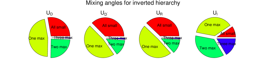
Fig. 9 shows the distribution of maximal mixing angles for the IH case. Note that one observes a similar distribution for NH neutrinos (cf. Fig. 6), namely that in most cases large leptonic mixing angles come from $U_{\ell}$. However, for IH neutrino masses, there is a slight tendency to larger mixing angles in $U_{D}$, $U_{D^{\prime}}$, and $U_{R}$, and smaller mixing angles in $U_{\ell}$ than in the NH case. The distribution of the special cases in Fig. 7 resembles that for the normal hierarchy. For example, $M_{R}$ is approximately diagonal in about 15% of all cases.

6.2 QD Spectrum

The case of QD neutrino masses is more tricky from the computational point of view because of redundancy. As a simple example, consider Eq. (20b) with $M_{\text{eff}}^{\text{diag}}=\mathbbm{1}$. In the real case, one can use any $\widehat{U}_{\text{PMNS}}$ and $\widehat{U}_{\ell}$ in this equation in order to obtain $M_{\text{eff}}^{\text{exp}}=\mathbbm{1}$, i.e., the different cases for $\widehat{U}_{\ell}$ are not really qualitatively different and a statistical analysis, such as above, does not make much sense. In addition, the matching to experiment (or the experimental data as a selection criterion) is, in this way, rather meaningless. From Eq. (24), one can read off that we require $M_{\text{eff}}^{\text{th}}\propto\mathbbm{1}+\mathcal{O}(\epsilon^{3})$. This implies that any realization producing $M_{\text{eff}}^{\text{th}}\simeq c\cdot\mathbbm{1}$ will be accepted by the algorithm, which are quite many. An interesting observation in the degenerate case, is that the realizations divide into two qualitatively different cases: the trivial case, i.e., $M_{D}=M_{R}=\mathbbm{1}$, and a large number of non-trivial cases. There is no such trivial case for IH neutrinos.

7 Summary and Conclusions

Quark-lepton unification generally leads to predictions in the patterns of the Yukawa coupling matrices of the fermions, which are often called “textures”. Because of the high dimension of the parameter space, a direct systematic study or scan of all valid textures at the level of the Yukawa couplings is difficult to perform. Therefore, we suggest a “bottom up” search strategy: We construct the parameter space of all valid textures from very generic (low-level) assumptions in the relevant leptonic mixing matrices and mass spectra. In this approach, we use the context of extended quark-lepton complementarity, which means that all mixing angles are either maximal or described by powers of $\epsilon\simeq\theta_{\text{C}}$. In addition, all mass ratios (of the neutrinos and charged leptons, as well as the mass hierarchies in $M_{D}$ and $M_{R}$) are also parameterized by powers $\epsilon$. This expansion parameter may be the remnant of a flavor symmetry describing the masses and mixing angles in both the quark and lepton sectors within a quark-lepton unified context. Note that in this setting, the solar neutrino mixing angle can only emerge as a combination of maximal mixing and $\theta_{\text{C}}$, i.e., our assumptions are somewhat more general than the usual QLC relations [see, e.g., Eq. (3)].

Our procedure, in short terms, is as follows (cf., Fig. 2): First, we systematically construct all combinatorial possibilities for all mixing matrices and mass spectra for the type-I seesaw mechanism up to the order $\epsilon^{2}$. In each case, we compute the effective neutrino mass matrix $M_{\mathrm{eff}}^{\text{th}}$ from that. In the second step, we determine all possibilities for $M_{\mathrm{eff}}^{\text{exp}}$ containing the experimental information from $U_{\text{PMNS}}$, the neutrino mass hierarchy, and $U_{\ell}$. In the third step, the two matrices are matched, i.e., the realizations compatible with current data are selected. Finally, we identify the leading order entries in the matrices, which lead to the sets of textures. We scan about 20 trillion possibilities focusing on the real, CP conserving case, and we mainly discuss a normal neutrino mass hierarchy. As an experimentally motivated input value for $\sin^{2}2\theta_{13}$, we take the current best-fit value $\sin^{2}2\theta_{13}=0$ as an example.

Compared to individual models in the literature, our assumptions are too generic to be able to predict the outcome a priori, which may reduce the bias. This key feature allows for the interpretation of the valid result statistics with respect to observables, constructed hierarchies, etc.. For example, we find many different cases with a very mild hierarchy in $M_{R}$ (with an abundance of about 80% in the textures), a result which does not involve any bias from the point of view of the assumptions. In addition, we find only very few cases with a symmetric Dirac neutrino mass matrix $M_{D}$ or small mixing ($U_{\ell}\simeq\mathbbm{1}$) in the charged lepton sector. However, we find a roughly diagonal right-handed neutrino mass matrix $M_{R}$ in relatively many cases, i.e., in about 24% of all realizations for the normal neutrino mass hierarchy. It would be interesting to investigate signals of lepton flavor violation for our list of matrices, and connect our results to statistical studies along the lines of Ref. [62] or to recent attempts of scanning the SM parameters including quark and lepton masses [63].

We have presented a complete selection of 72 examples for Yukawa coupling textures satisfying specific selection criteria. A more complete list of 1981 texture sets (obtained by relaxing the selection criteria) can be found in Ref. [60]. We have shown in two examples that the textures are very useful for a direct search for flavor symmetries predicting current data. Therefore, our list(s) of textures can be understood as an intermediate result from the point of view of model building. They might be used to systematically test and find flavor symmetries and allow for a more systematic approach to constructing models.

We conclude that systematic, machine-supported searches of parameter spaces related to model building may, in fact, open up new possibilities. While conventional approaches focus on individual models in greater depth, our approach produces all valid lepton mass matrices with the only bias of the (often very generic) input assumptions. Therefore, they allow for the identification of new possibilities, as well as for more general studies of the discussed parameter space. Hence, our study should not only be interpreted with respect to the input assumptions, but also with respect to the procedure itself.

Appendix A Details of the Procedure, Heuristics, and Complexity

In this appendix, we give details of the algorithm, heuristics (also physically relevant ones, everything which makes the algorithm faster but does not lead to a loss of generality), and complexity.

A.1 Parameter Space for the Mass Hierarchies

In the procedure described in Sec. 3.3, we have considered all possible diagonal mass matrices $M_{D}^{\text{diag}}=m_{D}\,\text{diag}(\epsilon^{a},\epsilon^{b},\epsilon^{c})$ and $M_{R}^{\text{diag}}=m_{D}\,\text{diag}(\epsilon^{a^{\prime}},\epsilon^{b^{\prime}},\epsilon^{c^{\prime}})$, with suitable non-negative integers $a,b,c,a^{\prime},b^{\prime},$ and $c^{\prime}$, that are compatible with the observed neutrino mass squared differences and leptonic mixing angles. As we will now see, the relevant range of these integers can actually be restricted considerably if we take the parameterization of the neutrino mass spectrum in Eq. (12) into account.

By factoring out common powers in $\epsilon$, we see that $M_{D}^{\text{diag}}$ and $M_{R}^{\text{diag}}$ can be written as

$$M_{D}^{\mathrm{diag}}=m_{D}\,\text{diag}(\epsilon^{m},\epsilon^{n},1),\quad M_{D}^{\mathrm{diag}}=m_{D}\,\text{diag}(\epsilon^{m},1,\epsilon^{n}),\quad M_{D}^{\mathrm{diag}}=m_{D}\,\text{diag}(1,\epsilon^{m},\epsilon^{n}),$$ (27a)

and

$$M_{R}^{\text{diag}}=M_{B-L}\,\mathrm{diag}(\epsilon^{p},\epsilon^{q},1)\>\>\text{with}\>\>0\leq q\leq p,$$ (27b)

where $$m,n,p q m_{D}\sim 10^{2}\>\text{GeV} M_{R}^{\text{diag}} 0\leq q\leq p M_{D}^{\text{diag}} M_{D}^{\text{diag}} m n n\leq m n>m m_{\nu}\equiv m_{D}^{2}/M_{B-L} m_{D}\sim 10^{2}\>\text{GeV} M_{B-L}\sim 10^{14}\>\text{GeV} m_{D}\rightarrow a\cdot m_{D} M_{B-L}\rightarrow a^{2}\cdot M_{R} a m_{\nu}\sim 10^{-2}\>\text{eV} \text{det}\,M_{\text{eff}}^{\text{diag}}=(\text{det}\,M_{D}^{\text{diag}})^{2}\text{det}\,(M_{R}^{\text{diag}})^{-1}$$, and , are non-negative integers, and . In Eq. (27b), we have made use of the possibility to bring to a strictly hierarchical form, which is expressed by the condition . One then has, however, no longer the freedom to choose the order of the mass eigenvalues of , and that is why Eq. (27a) includes all permutations of without any specific ordering of and , i.e., we allow in Eq. (27a) for both the cases and . In the following, we set . Although and would be preferred values, we can, of course, always rescale and by some factor , thereby leaving the absolute neutrino mass scale unchanged. From we find the relation

$$2(m+n)-p-q=k,$$ (27c)

where $k$ is a non-negative integer that depends on the type of neutrino mass spectrum in Eq. (12): We have $k=3$ for a normal, $k=1$ for an inverted, and $k=0$ for a degenerate neutrino mass spectrum.

We are now interested in determining the allowed ranges for the integers $m,n,p,$ and $q$, in Eqs. (27). Later, we will apply Eq. (24) up to order $\epsilon^{2}$, i.e., we will require a numerical matching precision $\mathcal{O}{(\epsilon^{3})}$ between $M_{\text{eff}}^{\text{th}}$ and $M_{\text{eff}}^{\text{exp}}$. From that matching precision it follows that only powers up to $\epsilon^{2}$ are relevant in the individual factors in the product Eq. (20a), because higher order terms will be absorbed by this matching uncertainty. The only non-trivial aspect in this argument is the factor $M_{R}^{-1}$. Let us write $(M_{R}^{\text{diag}})^{-1}=\epsilon^{-p}M_{B-L}^{-1}\,\text{diag}(1,\epsilon^{p-q},\epsilon^{p})$, and redefine $m_{D}\rightarrow\epsilon^{p/2}m_{D}$ and $M_{R}\rightarrow\epsilon^{p}M_{R}$, which leaves $m_{\nu}$ unaffected. Consider now the entries $\epsilon^{m}$, $\epsilon^{n}$, $\epsilon^{p-q}$, and $\epsilon^{p}$, in $M_{D}^{\text{diag}}$ and $(M_{R}^{\text{diag}})^{-1}$. If $m$, $n$, $p-q$, or $q$, are larger than 2, then the corresponding contribution to $M_{\text{eff}}$ will be absorbed in the matching precision. It follows that it is sufficient to restrict the maximum values of $m,m,p,$ and $q$ to 2, i.e., we need to consider for the powers of $\epsilon$ only

$$0\leq m,n,p,q\leq 2,$$ (28)

where we have used that $0\leq q\leq p$. The matrices $M_{D}^{\text{diag}}$ and $M_{R}^{\text{diag}}$ with higher powers of $\epsilon$ fall then into one of the classes already covered by a combination of powers satisfying Eq. (27c).

A.2 Matching of Matrices and the Absolute Neutrino Mass Scale

In this section, we describe the numerical implementation of Eq. (24): $M_{\text{eff}}^{\text{th}}|_{\epsilon=0.2}\simeq M_{\text{eff}}^{\text{exp}}|_{\epsilon=0.2}$. For our procedure, it makes sense to require a matching precision of $\mathcal{O}(\epsilon^{3})$ since $\epsilon^{2}$ is the maximum power that is used for the mass hierarchies and mixing angles (which was chosen because higher orders would be absorbed by the current measurement precision). This implies that a higher order matching precision will be too precise/restrictive because $\epsilon^{3}$ powers are not directly produced, and a lower order matching precision would not be able to distinguish cases differing by $\epsilon^{2}$-terms. Numerically, the $\mathcal{O}(\epsilon^{3})$ term can have any order one coefficient. We require a precision of $P=\epsilon^{3}$ for Eq. (24), which turns out to be reasonably restrictive by using actual tests, i.e., we require

$$(M_{\text{eff}}^{\text{exp}})_{ij}-P\leq c\cdot(M_{\text{eff}}^{\text{th}})_{ij}\leq(M_{\text{eff}}^{\text{exp}})_{ij}+P,$$ (29a)

with $$P=\epsilon^{3} c M_{R}$$ and is a constant which can be absorbed into (or can come from) the absolute mass scale, mixing angles, and the highest hierarchy power in .

In order to evaluate Eq. (29a), we have to determine $c$ in order to check whether $M_{\text{eff}}^{\text{th}}$ falls into the proper interval. Let us re-write Eq. (29a) as

$$(M_{\text{eff}}^{\mathrm{exp}})_{ij}^{\mathrm{low}}\leq c\cdot(M_{\text{eff}}^{\text{th}})_{ij}\leq(M_{\text{eff}}^{\mathrm{exp}})_{ij}^{\mathrm{up}}\,.$$ (29b)

This corresponds to 6$\times$2 independent inequalities. Dividing now these inequalities by $(M_{\text{eff}}^{\text{exp}})_{ij}$ gives

$$\frac{(M_{\text{eff}}^{\mathrm{exp}})_{ij}^{\mathrm{low}}}{(M_{\text{eff}}^{\text{th}})_{ij}}\leq c \leq\frac{(M_{\text{eff}}^{\mathrm{exp}})_{ij}^{\mathrm{up}}}{(M_{\text{eff}}^{\text{th}})_{ij}}\quad\mathrm{for}\,\,(M_{\text{eff}}^{\text{th}})_{ij}>0\,,$$

$$\frac{(M_{\text{eff}}^{\mathrm{exp}})_{ij}^{\mathrm{up}}}{(M_{\text{eff}}^{\text{th}})_{ij}}\leq c \leq\frac{(M_{\text{eff}}^{\mathrm{exp}})_{ij}^{\mathrm{low}}}{(M_{\text{eff}}^{\text{th}})_{ij}}\quad\mathrm{for}\,\,(M_{\text{eff}}^{\text{th}})_{ij}<0\,.$$ (29c)

Watch for the special case $(M_{\text{eff}})_{ij}=0$. The intersection of these intervals is then obtained as

$$\underbrace{\max\left(\frac{(M_{\text{eff}}^{\mathrm{exp}})_{ij}^{\mathrm{L}}}{(M_{\text{eff}}^{\text{th}})_{ij}}\right)}_{c^{L}}\leq c\leq\underbrace{\min\left(\frac{(M_{\text{eff}}^{\mathrm{exp}})_{ij}^{\mathrm{U}}}{(M_{\text{eff}}^{\text{th}})_{ij}}\right)}_{c^{U}}$$ (29d)

with $(M_{\text{eff}}^{\mathrm{exp}})_{ij}^{\mathrm{L}}$ and $(M_{\text{eff}}^{\mathrm{exp}})_{ij}^{\mathrm{U}}$ chosen according to the case selection in Eq. (29c) for $i$ and $j$ individually. Only, if $c^{L}\leq c^{U}$, then we have an allowed range for $c$. If, however, $c^{L}>c^{U}$, the realization is refused. Note that the constant $c$ is not used anymore further on since it may have different origins. However, the appropriate absolute mass scale will be implicitly determined in order to satisfy Eq. (24).

A.3 Complexity and Counting of Cases

In order to avoid in our procedure the generation of equivalent realizations and double-counting of cases, several heuristics can be used. As far as the phases in Eq. (20a) are concerned, we only have the matrices $D_{D}$, $\tilde{K}$, $\tilde{D}$ for the real case, which leads to $2^{(3+2+3)}=2^{8}=256$ phases. For $\theta_{13}^{x}=0$, the phase $\delta^{x}$ is unphysical, and we only test one case. This leads to $4^{6}\times(3\times 2+1)^{3}$ different angle combinations in $M_{\text{eff}}^{\text{th}}$. For $M_{\text{eff}}^{\text{exp}}$ in Eq. (20b), we do not generate $D_{\ell}$ in Eq. (20b), because the phases in the corresponding $D_{D}$ will match a valid case of $M_{\text{eff}}^{\text{exp}}$ since both matrices appear on the outside (a valid phase in $D_{D}$ then actually corresponds to two cases for $D_{D}$ and $D_{\ell}$). In the real case, we therefore have only $2^{2}=4$ phases from $K_{\ell}$, and $4^{2}\times(3\times 2+1)=112$ cases for the angles in $\widehat{U}_{\ell}$. This has to be multiplied with the corresponding allowed hierarchies in $M_{D}$ and $M_{R}$. It is easy to derive that there are 12 possible cases for a normal neutrino mass hierarchy, 9 possible cases for an inverted hierarchy, and 13 cases for the degenerate case (cf., Appendix A.1). In addition, we test six cases for the true values in $\widehat{U}_{\text{PMNS}}$. Since in the degenerate case any $\widehat{U}_{\ell}$ and any $\widehat{U}_{\text{PMNS}}$ leads to a diagonal $M_{\text{eff}}^{\text{exp}}$, it is sufficient to test one case for $\widehat{U}_{\ell}$ and $K_{\ell}$. This means that the degenerate case hardly contributes to the complexity. Further simplifications are possible for $M_{D}^{\text{diag}}=\mathbbm{1}$, etc.. In this case, one has to watch that the relative counting of different hierarchy/mixing angle cases is affected. In total, we test

$$N=256\times 4^{6}\times(3\times 2+1)^{3}\times\left(112\times 4\times(12+9)+13\right)\times 6\simeq 20\cdot 10^{12}$$ (30)

different combinatorial possibilities, which require about 2 months of running time on a modern computer using a C-based software.

The number of allowed combinations may be used as a statistical measure in some cases. The interpretation is then related to the number of different possibilities.

Appendix B Details of the Results for the NH Case

This section contains supplementary material for Sec. 5, such as the selection criteria used and the phases necessary for a complete reconstruction of the charged lepton and neutrino Yukawa couplings.

B.1 Texture Set Selection Criteria

Let us now describe the selection criteria leading to the texture sets presented in Sec. 5. In producing Table LABEL:tab:seesawtextures, we have used the following criteria:

1. The seesaw realizations should resist an increased experimental pressure provided that the current best-fit values are unchanged, i.e., $\sin^{2}2\theta_{13}$ will not be found. We impose an extrapolated experimental limit by using $\sigma_{12}\simeq 4.6\%$ [44] and $\sigma_{23}\simeq 10\%$ [43] in Eq. (26), which corresponds to about a decade from now. Since $\theta_{13}$ is in any case smaller than $1^{\circ}$ and would anyway resist an increased experimental pressure, we do not have to consider it for a further selection.

2. Textures that differ by entries of the order $\epsilon^{2}$ should be included with only one example. We choose the realization with the best $\chi^{2}$.

3. The selection of realizations should be stable under $\epsilon^{2}$-variations of the mixing angles, i.e., if we find mixing angles $\epsilon^{2}$, the realization has to be valid for $\epsilon^{2}\rightarrow 0$ as well. We include the newly obtained texture sets in Table LABEL:tab:seesawtextures by introducing the angle $\xi\in\{0,\epsilon^{2}\}$. Note that these cases are initially generated as well, but they might be filtered out later by Eq. (24).

4. We omit texture sets with anarchical $M_{R}$ (matrices just filled with entries “1”), since such structure-less textures do, in general, not yield much useful information.

5. We also show only one example for each texture set $(M_{1},M_{2},M_{3})\sim(M_{\ell},M_{D},M_{R})$, where $M_{i}$ ($i=1,2,3$) are the corresponding textures obtained after texture reduction, which have one pair $\{M_{j},M_{k}\}$ appearing together with more than one possible $M_{i}$ ($i\neq j\neq k$). In this case, we keep the texture set associated with a representation that has the lowest $\chi^{2}$.

By using the above selection criteria, we obtain the list of 72 texture sets shown in Tables LABEL:tab:seesawtextures and LABEL:tab:seesawtexturesphases. The effects of the different selection criteria on the number of texture sets is shown in Table 4. In this table, we also show the numbers of distinct textures for $M_{\ell}$, $M_{D}$ and $M_{R}$.

Selection criterion	#Textures	$\#M_{\ell}$	$\#M_{D}$	$\#M_{R}$
None	1 981	20	621	35
1.–2.	1 048	20	475	31
1.–3.	447	20	270	22
1.–5.	72	17	65	21

Table 4: Total number of texture sets, and the numbers of distinct textures for $M_{\ell}$, $M_{D}$ and $M_{R}$. Each row corresponds to the application of the selection criteria specified in the first column (see text).

B.2 Supplementary Information for the Texture Sets

Table LABEL:tab:seesawtexturesphases shows extra details of the realizations listed in Table LABEL:tab:seesawtextures. It contains the complete set of phases, the PMNS mixing angles, $\chi^{2}$ (in the 10 years limit, cf., App. B.1), and the number of realizations leading to each texture set (for $\xi=\epsilon^{2}$ in ambiguous cases). Note that we chose $\varphi^{D^{\prime}}_{1}=\varphi^{D^{\prime}}_{2}=\varphi^{D^{\prime}}_{3}=\alpha^{D}_{1}=\alpha^{D}_{2}=0$ since these phases appear in $M_{\text{eff}}^{\text{th}}$ only in combination with other phases (see Eq. (20)), and can be absorbed into the other phases. Tables LABEL:tab:seesawtextures and LABEL:tab:seesawtexturesphases provide together the complete information sufficient to fully reconstruct the Yukawa coupling matrices of the 72 realizations.

Table 5: Supplementary information for Table LABEL:tab:seesawtextures ($\varphi^{D^{\prime}}_{1,2,3}=\alpha^{D}_{1,2}=0$) (see text).

#	$(\delta^{l},\alpha_{1}^{l},\alpha_{2}^{l})$	$(\delta^{D},\varphi_{1}^{D},\varphi_{2}^{D},\varphi_{3}^{D})$	$(\delta^{D^{\prime}},\alpha_{1}^{D^{\prime}},\alpha_{2}^{D^{\prime}})$	$(\delta^{R},\varphi_{1}^{R},\varphi_{2}^{R},\varphi_{3}^{R})$	$(\theta_{12},\theta_{13},\theta_{23})$	$\chi^{2}$	Cases
$1$	$\par\begin{array}[]{c}(0,\pi,0)\end{array}$	$\begin{array}[]{c}(\pi,0,0,\pi)\end{array}$	$\begin{array}[]{c}(\pi,\pi,\pi)\end{array}$	$\begin{array}[]{c}(0,0,0,\pi)\end{array}$	$\begin{array}[]{c}(34.0^{\circ},0.2^{\circ},52.2^{\circ})\end{array}$	$7.12$	18
$2$	$\par\begin{array}[]{c}(\pi,0,\pi)\end{array}$	$\begin{array}[]{c}(\pi,0,0,\pi)\end{array}$	$\begin{array}[]{c}(0,0,\pi)\end{array}$	$\begin{array}[]{c}(\pi,0,\pi,\pi)\end{array}$	$\begin{array}[]{c}(33.6^{\circ},0.2^{\circ},51.5^{\circ})\end{array}$	$5.29$	38
$3$	$\par\begin{array}[]{c}(\pi,0,0)\end{array}$	$\begin{array}[]{c}(0,0,\pi,0)\end{array}$	$\begin{array}[]{c}(0,0,0)\end{array}$	$\begin{array}[]{c}(\pi,0,\pi,0)\end{array}$	$\begin{array}[]{c}(33.5^{\circ},0.2^{\circ},51.3^{\circ})\end{array}$	$4.9$	26
$4$	$\par\begin{array}[]{c}(0,0,\pi)\end{array}$	$\begin{array}[]{c}(0,0,0,\pi)\end{array}$	$\begin{array}[]{c}(\pi,0,\pi)\end{array}$	$\begin{array}[]{c}(\pi,0,\pi,\pi)\end{array}$	$\begin{array}[]{c}(33.5^{\circ},0.1^{\circ},51.2^{\circ})\end{array}$	$4.71$	17
$5$	$\par\begin{array}[]{c}(0,0,0)\end{array}$	$\begin{array}[]{c}(0,0,0,0)\end{array}$	$\begin{array}[]{c}(0,\pi,0)\end{array}$	$\begin{array}[]{c}(0,0,0,\pi)\end{array}$	$\begin{array}[]{c}(33.0^{\circ},0.4^{\circ},51.2^{\circ})\end{array}$	$4.7$	17
$6$	$\par\begin{array}[]{c}(\pi,\pi,0)\end{array}$	$\begin{array}[]{c}(\pi,0,0,0)\end{array}$	$\begin{array}[]{c}(\pi,\pi,\pi)\end{array}$	$\begin{array}[]{c}(0,0,0,0)\end{array}$	$\begin{array}[]{c}(33.3^{\circ},0.4^{\circ},51.2^{\circ})\end{array}$	$4.7$	177
$7$	$\par\begin{array}[]{c}(\pi,\pi,0)\end{array}$	$\begin{array}[]{c}(\pi,0,0,0)\end{array}$	$\begin{array}[]{c}(0,0,0)\end{array}$	$\begin{array}[]{c}(\pi,0,0,0)\end{array}$	$\begin{array}[]{c}(33.3^{\circ},0.4^{\circ},51.2^{\circ})\end{array}$	$4.7$	63
$8$	$\par\begin{array}[]{c}(0,0,\pi)\end{array}$	$\begin{array}[]{c}(0,0,0,\pi)\end{array}$	$\begin{array}[]{c}(0,\pi,0)\end{array}$	$\begin{array}[]{c}(0,0,\pi,\pi)\end{array}$	$\begin{array}[]{c}(33.5^{\circ},0.1^{\circ},51.2^{\circ})\end{array}$	$4.71$	17
$9$	$\par\begin{array}[]{c}(\pi,\pi,\pi)\end{array}$	$\begin{array}[]{c}(0,0,\pi,0)\end{array}$	$\begin{array}[]{c}(\pi,0,0)\end{array}$	$\begin{array}[]{c}(0,0,\pi,0)\end{array}$	$\begin{array}[]{c}(32.9^{\circ},0.2^{\circ},51.2^{\circ})\end{array}$	$4.76$	23
$10$	$\par\begin{array}[]{c}(\pi,0,0)\end{array}$	$\begin{array}[]{c}(\pi,0,0,\pi)\end{array}$	$\begin{array}[]{c}(0,0,0)\end{array}$	$\begin{array}[]{c}(0,0,0,\pi)\end{array}$	$\begin{array}[]{c}(33.2^{\circ},0.2^{\circ},51.3^{\circ})\end{array}$	$4.78$	597
$11$	$\par\begin{array}[]{c}(\pi,0,0)\end{array}$	$\begin{array}[]{c}(\pi,0,0,\pi)\end{array}$	$\begin{array}[]{c}(0,0,0)\end{array}$	$\begin{array}[]{c}(0,0,0,\pi)\end{array}$	$\begin{array}[]{c}(33.2^{\circ},0.2^{\circ},51.3^{\circ})\end{array}$	$4.78$	835
$12$	$\par\begin{array}[]{c}(0,\pi,\pi)\end{array}$	$\begin{array}[]{c}(0,0,0,0)\end{array}$	$\begin{array}[]{c}(0,\pi,0)\end{array}$	$\begin{array}[]{c}(\pi,0,0,\pi)\end{array}$	$\begin{array}[]{c}(33.4^{\circ},0.0^{\circ},51.3^{\circ})\end{array}$	$4.81$	475
$13$	$\par\begin{array}[]{c}(0,0,0)\end{array}$	$\begin{array}[]{c}(\pi,0,0,\pi)\end{array}$	$\begin{array}[]{c}(0,0,0)\end{array}$	$\begin{array}[]{c}(\pi,0,0,0)\end{array}$	$\begin{array}[]{c}(33.4^{\circ},0.2^{\circ},51.3^{\circ})\end{array}$	$4.84$	104
$14$	$\par\begin{array}[]{c}(\pi,0,0)\end{array}$	$\begin{array}[]{c}(\pi,0,\pi,0)\end{array}$	$\begin{array}[]{c}(\pi,\pi,0)\end{array}$	$\begin{array}[]{c}(0,0,0,\pi)\end{array}$	$\begin{array}[]{c}(33.5^{\circ},0.6^{\circ},51.3^{\circ})\end{array}$	$4.89$	14
$15$	$\par\begin{array}[]{c}(\pi,0,0)\end{array}$	$\begin{array}[]{c}(0,0,\pi,0)\end{array}$	$\begin{array}[]{c}(0,0,0)\end{array}$	$\begin{array}[]{c}(\pi,0,\pi,0)\end{array}$	$\begin{array}[]{c}(33.5^{\circ},0.2^{\circ},51.3^{\circ})\end{array}$	$4.9$	17
$16$	$\par\begin{array}[]{c}(\pi,0,0)\end{array}$	$\begin{array}[]{c}(\pi,0,\pi,0)\end{array}$	$\begin{array}[]{c}(0,\pi,0)\end{array}$	$\begin{array}[]{c}(0,0,0,\pi)\end{array}$	$\begin{array}[]{c}(33.5^{\circ},0.6^{\circ},51.3^{\circ})\end{array}$	$4.9$	120
$17$	$\par\begin{array}[]{c}(\pi,0,0)\end{array}$	$\begin{array}[]{c}(\pi,0,0,0)\end{array}$	$\begin{array}[]{c}(0,0,\pi)\end{array}$	$\begin{array}[]{c}(\pi,0,0,\pi)\end{array}$	$\begin{array}[]{c}(33.3^{\circ},0.0^{\circ},51.4^{\circ})\end{array}$	$4.96$	1138
$18$	$\par\begin{array}[]{c}(0,\pi,\pi)\end{array}$	$\begin{array}[]{c}(0,0,\pi,\pi)\end{array}$	$\begin{array}[]{c}(0,\pi,\pi)\end{array}$	$\begin{array}[]{c}(0,0,\pi,\pi)\end{array}$	$\begin{array}[]{c}(33.5^{\circ},0.2^{\circ},51.4^{\circ})\end{array}$	$4.97$	9
$19$	$\par\begin{array}[]{c}(0,\pi,\pi)\end{array}$	$\begin{array}[]{c}(0,0,0,0)\end{array}$	$\begin{array}[]{c}(0,0,0)\end{array}$	$\begin{array}[]{c}(0,0,0,0)\end{array}$	$\begin{array}[]{c}(33.4^{\circ},0.0^{\circ},51.4^{\circ})\end{array}$	$4.99$	387
$20$	$\par\begin{array}[]{c}(\pi,0,\pi)\end{array}$	$\begin{array}[]{c}(\pi,0,0,0)\end{array}$	$\begin{array}[]{c}(0,\pi,0)\end{array}$	$\begin{array}[]{c}(0,0,\pi,\pi)\end{array}$	$\begin{array}[]{c}(33.7^{\circ},0.2^{\circ},51.2^{\circ})\end{array}$	$5.02$	26
$21$	$\par\begin{array}[]{c}(\pi,0,0)\end{array}$	$\begin{array}[]{c}(0,0,0,\pi)\end{array}$	$\begin{array}[]{c}(0,0,0)\end{array}$	$\begin{array}[]{c}(0,0,0,\pi)\end{array}$	$\begin{array}[]{c}(33.4^{\circ},0.1^{\circ},51.5^{\circ})\end{array}$	$5.03$	776
$22$	$\par\begin{array}[]{c}(\pi,0,0)\end{array}$	$\begin{array}[]{c}(0,0,0,\pi)\end{array}$	$\begin{array}[]{c}(0,0,\pi)\end{array}$	$\begin{array}[]{c}(\pi,0,\pi,\pi)\end{array}$	$\begin{array}[]{c}(33.2^{\circ},0.1^{\circ},51.5^{\circ})\end{array}$	$5.03$	876
$23$	$\par\begin{array}[]{c}(\pi,0,0)\end{array}$	$\begin{array}[]{c}(0,0,0,\pi)\end{array}$	$\begin{array}[]{c}(\pi,\pi,0)\end{array}$	$\begin{array}[]{c}(0,0,\pi,\pi)\end{array}$	$\begin{array}[]{c}(33.2^{\circ},0.1^{\circ},51.5^{\circ})\end{array}$	$5.03$	1351
$24$	$\par\begin{array}[]{c}(\pi,\pi,\pi)\end{array}$	$\begin{array}[]{c}(0,0,\pi,0)\end{array}$	$\begin{array}[]{c}(0,\pi,\pi)\end{array}$	$\begin{array}[]{c}(\pi,0,\pi,\pi)\end{array}$	$\begin{array}[]{c}(33.5^{\circ},0.3^{\circ},51.4^{\circ})\end{array}$	$5.05$	27
$25$	$\par\begin{array}[]{c}(\pi,0,0)\end{array}$	$\begin{array}[]{c}(0,0,\pi,0)\end{array}$	$\begin{array}[]{c}(\pi,\pi,0)\end{array}$	$\begin{array}[]{c}(0,0,0,\pi)\end{array}$	$\begin{array}[]{c}(33.5^{\circ},0.1^{\circ},51.4^{\circ})\end{array}$	$5.06$	392
$26$	$\par\begin{array}[]{c}(\pi,0,0)\end{array}$	$\begin{array}[]{c}(0,0,0,\pi)\end{array}$	$\begin{array}[]{c}(0,0,0)\end{array}$	$\begin{array}[]{c}(0,0,0,\pi)\end{array}$	$\begin{array}[]{c}(33.4^{\circ},0.1^{\circ},51.5^{\circ})\end{array}$	$5.09$	307
$27$	$\par\begin{array}[]{c}(0,0,\pi)\end{array}$	$\begin{array}[]{c}(0,0,0,\pi)\end{array}$	$\begin{array}[]{c}(0,\pi,0)\end{array}$	$\begin{array}[]{c}(0,0,\pi,0)\end{array}$	$\begin{array}[]{c}(33.5^{\circ},0.2^{\circ},51.4^{\circ})\end{array}$	$5.09$	26
$28$	$\par\begin{array}[]{c}(\pi,0,0)\end{array}$	$\begin{array}[]{c}(0,0,\pi,0)\end{array}$	$\begin{array}[]{c}(\pi,0,0)\end{array}$	$\begin{array}[]{c}(\pi,0,\pi,0)\end{array}$	$\begin{array}[]{c}(33.7^{\circ},0.2^{\circ},51.3^{\circ})\end{array}$	$5.11$	296
$29$	$\par\begin{array}[]{c}(\pi,0,\pi)\end{array}$	$\begin{array}[]{c}(\pi,0,0,\pi)\end{array}$	$\begin{array}[]{c}(\pi,\pi,\pi)\end{array}$	$\begin{array}[]{c}(0,0,0,\pi)\end{array}$	$\begin{array}[]{c}(33.6^{\circ},0.2^{\circ},51.4^{\circ})\end{array}$	$5.16$	5
$30$	$\par\begin{array}[]{c}(\pi,0,\pi)\end{array}$	$\begin{array}[]{c}(\pi,0,0,\pi)\end{array}$	$\begin{array}[]{c}(\pi,\pi,\pi)\end{array}$	$\begin{array}[]{c}(0,0,0,\pi)\end{array}$	$\begin{array}[]{c}(33.6^{\circ},0.2^{\circ},51.4^{\circ})\end{array}$	$5.16$	5
$31$	$\par\begin{array}[]{c}(\pi,0,\pi)\end{array}$	$\begin{array}[]{c}(\pi,0,0,\pi)\end{array}$	$\begin{array}[]{c}(0,0,\pi)\end{array}$	$\begin{array}[]{c}(\pi,0,\pi,\pi)\end{array}$	$\begin{array}[]{c}(33.6^{\circ},0.2^{\circ},51.5^{\circ})\end{array}$	$5.29$	38
$32$	$\par\begin{array}[]{c}(\pi,0,0)\end{array}$	$\begin{array}[]{c}(0,0,\pi,0)\end{array}$	$\begin{array}[]{c}(0,\pi,\pi)\end{array}$	$\begin{array}[]{c}(\pi,0,0,\pi)\end{array}$	$\begin{array}[]{c}(33.3^{\circ},0.2^{\circ},51.7^{\circ})\end{array}$	$5.31$	343
$33$	$\par\begin{array}[]{c}(\pi,\pi,\pi)\end{array}$	$\begin{array}[]{c}(\pi,0,0,0)\end{array}$	$\begin{array}[]{c}(0,0,0)\end{array}$	$\begin{array}[]{c}(0,0,\pi,0)\end{array}$	$\begin{array}[]{c}(33.6^{\circ},0.1^{\circ},51.5^{\circ})\end{array}$	$5.31$	83
$34$	$\par\begin{array}[]{c}(\pi,\pi,\pi)\end{array}$	$\begin{array}[]{c}(\pi,0,0,0)\end{array}$	$\begin{array}[]{c}(0,0,0)\end{array}$	$\begin{array}[]{c}(0,0,\pi,0)\end{array}$	$\begin{array}[]{c}(33.6^{\circ},0.1^{\circ},51.5^{\circ})\end{array}$	$5.31$	81
$35$	$\par\begin{array}[]{c}(0,\pi,0)\end{array}$	$\begin{array}[]{c}(\pi,0,0,\pi)\end{array}$	$\begin{array}[]{c}(0,\pi,0)\end{array}$	$\begin{array}[]{c}(\pi,0,\pi,0)\end{array}$	$\begin{array}[]{c}(33.7^{\circ},0.1^{\circ},51.5^{\circ})\end{array}$	$5.32$	143
$36$	$\par\begin{array}[]{c}(\pi,0,\pi)\end{array}$	$\begin{array}[]{c}(\pi,0,0,\pi)\end{array}$	$\begin{array}[]{c}(\pi,0,0)\end{array}$	$\begin{array}[]{c}(0,0,0,\pi)\end{array}$	$\begin{array}[]{c}(32.9^{\circ},0.2^{\circ},51.6^{\circ})\end{array}$	$5.33$	17
$37$	$\par\begin{array}[]{c}(\pi,0,\pi)\end{array}$	$\begin{array}[]{c}(\pi,0,0,\pi)\end{array}$	$\begin{array}[]{c}(0,\pi,\pi)\end{array}$	$\begin{array}[]{c}(0,0,0,0)\end{array}$	$\begin{array}[]{c}(32.9^{\circ},0.2^{\circ},51.6^{\circ})\end{array}$	$5.33$	17
$38$	$\par\begin{array}[]{c}(\pi,0,0)\end{array}$	$\begin{array}[]{c}(0,0,0,\pi)\end{array}$	$\begin{array}[]{c}(\pi,0,0)\end{array}$	$\begin{array}[]{c}(0,0,0,\pi)\end{array}$	$\begin{array}[]{c}(33.2^{\circ},0.1^{\circ},51.7^{\circ})\end{array}$	$5.33$	17
$39$	$\par\begin{array}[]{c}(\pi,0,0)\end{array}$	$\begin{array}[]{c}(0,0,0,\pi)\end{array}$	$\begin{array}[]{c}(\pi,0,0)\end{array}$	$\begin{array}[]{c}(0,0,0,\pi)\end{array}$	$\begin{array}[]{c}(33.2^{\circ},0.1^{\circ},51.7^{\circ})\end{array}$	$5.33$	33
$40$	$\par\begin{array}[]{c}(\pi,0,0)\end{array}$	$\begin{array}[]{c}(0,0,0,0)\end{array}$	$\begin{array}[]{c}(0,0,\pi)\end{array}$	$\begin{array}[]{c}(\pi,0,0,\pi)\end{array}$	$\begin{array}[]{c}(33.2^{\circ},0.1^{\circ},51.7^{\circ})\end{array}$	$5.37$	17
$41$	$\par\begin{array}[]{c}(\pi,0,\pi)\end{array}$	$\begin{array}[]{c}(\pi,0,0,\pi)\end{array}$	$\begin{array}[]{c}(\pi,0,0)\end{array}$	$\begin{array}[]{c}(0,0,\pi,\pi)\end{array}$	$\begin{array}[]{c}(33.1^{\circ},0.0^{\circ},51.8^{\circ})\end{array}$	$5.47$	26
$42$	$\par\begin{array}[]{c}(\pi,0,\pi)\end{array}$	$\begin{array}[]{c}(\pi,0,0,\pi)\end{array}$	$\begin{array}[]{c}(0,\pi,\pi)\end{array}$	$\begin{array}[]{c}(0,0,0,\pi)\end{array}$	$\begin{array}[]{c}(33.1^{\circ},0.0^{\circ},51.8^{\circ})\end{array}$	$5.47$	17
$43$	$\par\begin{array}[]{c}(0,0,\pi)\end{array}$	$\begin{array}[]{c}(\pi,0,\pi,0)\end{array}$	$\begin{array}[]{c}(\pi,0,0)\end{array}$	$\begin{array}[]{c}(0,0,0,\pi)\end{array}$	$\begin{array}[]{c}(33.3^{\circ},0.2^{\circ},51.8^{\circ})\end{array}$	$5.48$	5
$44$	$\par\begin{array}[]{c}(0,0,\pi)\end{array}$	$\begin{array}[]{c}(\pi,0,\pi,0)\end{array}$	$\begin{array}[]{c}(\pi,0,0)\end{array}$	$\begin{array}[]{c}(0,0,0,\pi)\end{array}$	$\begin{array}[]{c}(33.3^{\circ},0.2^{\circ},51.8^{\circ})\end{array}$	$5.48$	14
$45$	$\par\begin{array}[]{c}(\pi,0,\pi)\end{array}$	$\begin{array}[]{c}(\pi,0,0,\pi)\end{array}$	$\begin{array}[]{c}(0,\pi,\pi)\end{array}$	$\begin{array}[]{c}(\pi,0,\pi,\pi)\end{array}$	$\begin{array}[]{c}(34.0^{\circ},0.3^{\circ},51.3^{\circ})\end{array}$	$5.66$	18
$46$	$\par\begin{array}[]{c}(0,0,0)\end{array}$	$\begin{array}[]{c}(\pi,0,0,\pi)\end{array}$	$\begin{array}[]{c}(0,0,0)\end{array}$	$\begin{array}[]{c}(\pi,0,0,\pi)\end{array}$	$\begin{array}[]{c}(33.9^{\circ},0.7^{\circ},51.5^{\circ})\end{array}$	$5.84$	5
$47$	$\par\begin{array}[]{c}(0,0,0)\end{array}$	$\begin{array}[]{c}(\pi,0,0,\pi)\end{array}$	$\begin{array}[]{c}(\pi,0,0)\end{array}$	$\begin{array}[]{c}(0,0,0,0)\end{array}$	$\begin{array}[]{c}(34.0^{\circ},0.7^{\circ},51.5^{\circ})\end{array}$	$5.96$	5
$48$	$\par\begin{array}[]{c}(\pi,\pi,\pi)\end{array}$	$\begin{array}[]{c}(0,0,0,\pi)\end{array}$	$\begin{array}[]{c}(0,\pi,\pi)\end{array}$	$\begin{array}[]{c}(0,0,0,0)\end{array}$	$\begin{array}[]{c}(33.7^{\circ},0.1^{\circ},51.9^{\circ})\end{array}$	$5.98$	9
$49$	$\par\begin{array}[]{c}(\pi,0,\pi)\end{array}$	$\begin{array}[]{c}(\pi,0,0,0)\end{array}$	$\begin{array}[]{c}(\pi,\pi,\pi)\end{array}$	$\begin{array}[]{c}(0,0,0,\pi)\end{array}$	$\begin{array}[]{c}(33.5^{\circ},0.4^{\circ},52.0^{\circ})\end{array}$	$6.02$	34
$50$	$\par\begin{array}[]{c}(\pi,0,\pi)\end{array}$	$\begin{array}[]{c}(\pi,0,0,0)\end{array}$	$\begin{array}[]{c}(0,0,0)\end{array}$	$\begin{array}[]{c}(\pi,0,\pi,0)\end{array}$	$\begin{array}[]{c}(33.5^{\circ},0.4^{\circ},52.0^{\circ})\end{array}$	$6.02$	26
$51$	$\par\begin{array}[]{c}(\pi,0,\pi)\end{array}$	$\begin{array}[]{c}(0,0,0,0)\end{array}$	$\begin{array}[]{c}(\pi,0,0)\end{array}$	$\begin{array}[]{c}(0,0,0,\pi)\end{array}$	$\begin{array}[]{c}(33.8^{\circ},0.3^{\circ},51.9^{\circ})\end{array}$	$6.19$	86
$52$	$\par\begin{array}[]{c}(\pi,0,\pi)\end{array}$	$\begin{array}[]{c}(0,0,0,0)\end{array}$	$\begin{array}[]{c}(\pi,0,0)\end{array}$	$\begin{array}[]{c}(0,0,0,\pi)\end{array}$	$\begin{array}[]{c}(33.8^{\circ},0.3^{\circ},51.9^{\circ})\end{array}$	$6.19$	87
$53$	$\par\begin{array}[]{c}(\pi,0,\pi)\end{array}$	$\begin{array}[]{c}(0,0,0,0)\end{array}$	$\begin{array}[]{c}(0,\pi,\pi)\end{array}$	$\begin{array}[]{c}(0,0,\pi,\pi)\end{array}$	$\begin{array}[]{c}(33.8^{\circ},0.3^{\circ},51.9^{\circ})\end{array}$	$6.19$	108
$54$	$\par\begin{array}[]{c}(0,0,0)\end{array}$	$\begin{array}[]{c}(0,0,\pi,\pi)\end{array}$	$\begin{array}[]{c}(0,\pi,\pi)\end{array}$	$\begin{array}[]{c}(0,0,\pi,\pi)\end{array}$	$\begin{array}[]{c}(34.4^{\circ},0.1^{\circ},51.1^{\circ})\end{array}$	$6.26$	14
$55$	$\par\begin{array}[]{c}(\pi,\pi,\pi)\end{array}$	$\begin{array}[]{c}(\pi,0,\pi,\pi)\end{array}$	$\begin{array}[]{c}(0,0,0)\end{array}$	$\begin{array}[]{c}(0,0,\pi,\pi)\end{array}$	$\begin{array}[]{c}(34.4^{\circ},0.1^{\circ},51.1^{\circ})\end{array}$	$6.26$	14
$56$	$\par\begin{array}[]{c}(0,0,0)\end{array}$	$\begin{array}[]{c}(\pi,0,0,\pi)\end{array}$	$\begin{array}[]{c}(\pi,\pi,0)\end{array}$	$\begin{array}[]{c}(\pi,0,0,\pi)\end{array}$	$\begin{array}[]{c}(32.5^{\circ},0.2^{\circ},52.0^{\circ})\end{array}$	$6.44$	79
$57$	$\par\begin{array}[]{c}(0,0,0)\end{array}$	$\begin{array}[]{c}(\pi,0,0,\pi)\end{array}$	$\begin{array}[]{c}(\pi,\pi,0)\end{array}$	$\begin{array}[]{c}(\pi,0,0,\pi)\end{array}$	$\begin{array}[]{c}(32.5^{\circ},0.2^{\circ},52.0^{\circ})\end{array}$	$6.44$	34
$58$	$\par\begin{array}[]{c}(0,\pi,\pi)\end{array}$	$\begin{array}[]{c}(\pi,0,0,\pi)\end{array}$	$\begin{array}[]{c}(0,0,0)\end{array}$	$\begin{array}[]{c}(0,0,\pi,0)\end{array}$	$\begin{array}[]{c}(34.2^{\circ},0.7^{\circ},51.5^{\circ})\end{array}$	$6.46$	5
$59$	$\par\begin{array}[]{c}(0,\pi,0)\end{array}$	$\begin{array}[]{c}(0,0,\pi,0)\end{array}$	$\begin{array}[]{c}(0,0,\pi)\end{array}$	$\begin{array}[]{c}(0,0,0,\pi)\end{array}$	$\begin{array}[]{c}(34.0^{\circ},0.2^{\circ},52.0^{\circ})\end{array}$	$6.59$	5
$60$	$\par\begin{array}[]{c}(0,0,0)\end{array}$	$\begin{array}[]{c}(\pi,0,0,\pi)\end{array}$	$\begin{array}[]{c}(\pi,0,\pi)\end{array}$	$\begin{array}[]{c}(0,0,0,\pi)\end{array}$	$\begin{array}[]{c}(34.0^{\circ},0.4^{\circ},52.0^{\circ})\end{array}$	$6.77$	5
$61$	$\par\begin{array}[]{c}(0,\pi,0)\end{array}$	$\begin{array}[]{c}(\pi,0,0,\pi)\end{array}$	$\begin{array}[]{c}(0,0,0)\end{array}$	$\begin{array}[]{c}(0,0,\pi,0)\end{array}$	$\begin{array}[]{c}(34.0^{\circ},0.2^{\circ},52.2^{\circ})\end{array}$	$7.12$	18
$62$	$\par\begin{array}[]{c}(0,\pi,0)\end{array}$	$\begin{array}[]{c}(\pi,0,0,\pi)\end{array}$	$\begin{array}[]{c}(\pi,\pi,\pi)\end{array}$	$\begin{array}[]{c}(0,0,0,\pi)\end{array}$	$\begin{array}[]{c}(34.0^{\circ},0.2^{\circ},52.2^{\circ})\end{array}$	$7.12$	18
$63$	$\par\begin{array}[]{c}(0,\pi,0)\end{array}$	$\begin{array}[]{c}(\pi,0,0,\pi)\end{array}$	$\begin{array}[]{c}(0,0,0)\end{array}$	$\begin{array}[]{c}(0,0,\pi,0)\end{array}$	$\begin{array}[]{c}(34.0^{\circ},0.2^{\circ},52.2^{\circ})\end{array}$	$7.12$	18
$64$	$\par\begin{array}[]{c}(\pi,\pi,\pi)\end{array}$	$\begin{array}[]{c}(\pi,0,0,0)\end{array}$	$\begin{array}[]{c}(0,0,\pi)\end{array}$	$\begin{array}[]{c}(0,0,\pi,\pi)\end{array}$	$\begin{array}[]{c}(34.1^{\circ},0.2^{\circ},52.2^{\circ})\end{array}$	$7.25$	17
$65$	$\par\begin{array}[]{c}(\pi,0,\pi)\end{array}$	$\begin{array}[]{c}(0,0,\pi,\pi)\end{array}$	$\begin{array}[]{c}(0,0,\pi)\end{array}$	$\begin{array}[]{c}(0,0,0,0)\end{array}$	$\begin{array}[]{c}(34.5^{\circ},0.3^{\circ},51.8^{\circ})\end{array}$	$7.84$	9
$66$	$\par\begin{array}[]{c}(0,\pi,0)\end{array}$	$\begin{array}[]{c}(\pi,0,\pi,\pi)\end{array}$	$\begin{array}[]{c}(0,\pi,0)\end{array}$	$\begin{array}[]{c}(0,0,0,0)\end{array}$	$\begin{array}[]{c}(34.5^{\circ},0.3^{\circ},51.8^{\circ})\end{array}$	$7.84$	9
$67$	$\par\begin{array}[]{c}(\pi,\pi,\pi)\end{array}$	$\begin{array}[]{c}(0,0,0,0)\end{array}$	$\begin{array}[]{c}(0,\pi,\pi)\end{array}$	$\begin{array}[]{c}(0,0,\pi,\pi)\end{array}$	$\begin{array}[]{c}(34.9^{\circ},0.4^{\circ},51.8^{\circ})\end{array}$	$9.31$	26
$68$	$\par\begin{array}[]{c}(\pi,\pi,\pi)\end{array}$	$\begin{array}[]{c}(0,0,0,0)\end{array}$	$\begin{array}[]{c}(\pi,0,0)\end{array}$	$\begin{array}[]{c}(0,0,0,0)\end{array}$	$\begin{array}[]{c}(34.9^{\circ},0.4^{\circ},51.8^{\circ})\end{array}$	$9.31$	31
$69$	$\par\begin{array}[]{c}(0,0,0)\end{array}$	$\begin{array}[]{c}(\pi,0,0,0)\end{array}$	$\begin{array}[]{c}(0,0,0)\end{array}$	$\begin{array}[]{c}(0,0,\pi,\pi)\end{array}$	$\begin{array}[]{c}(34.9^{\circ},0.4^{\circ},51.8^{\circ})\end{array}$	$9.31$	26
$70$	$\par\begin{array}[]{c}(0,0,0)\end{array}$	$\begin{array}[]{c}(\pi,0,0,0)\end{array}$	$\begin{array}[]{c}(\pi,\pi,\pi)\end{array}$	$\begin{array}[]{c}(0,0,0,0)\end{array}$	$\begin{array}[]{c}(34.9^{\circ},0.4^{\circ},51.8^{\circ})\end{array}$	$9.31$	31
$71$	$\par\begin{array}[]{c}(0,0,0)\end{array}$	$\begin{array}[]{c}(\pi,0,0,0)\end{array}$	$\begin{array}[]{c}(0,\pi,0)\end{array}$	$\begin{array}[]{c}(0,0,\pi,0)\end{array}$	$\begin{array}[]{c}(35.3^{\circ},0.3^{\circ},51.3^{\circ})\end{array}$	$10.73$	17
$72$	$\par\begin{array}[]{c}(0,0,0)\end{array}$	$\begin{array}[]{c}(\pi,0,0,0)\end{array}$	$\begin{array}[]{c}(0,\pi,0)\end{array}$	$\begin{array}[]{c}(0,0,\pi,0)\end{array}$	$\begin{array}[]{c}(35.3^{\circ},0.3^{\circ},51.3^{\circ})\end{array}$	$10.73$	17

References

- [1] S. Fukuda et al. (Super-Kamiokande), Phys. Lett. B539, 179 (2002), hep-ex/0205075.
- [2] Q. R. Ahmad et al. (SNO), Phys. Rev. Lett. 89, 011302 (2002), nucl-ex/0204009.
- [3] Y. Fukuda et al. (Super-Kamiokande), Phys. Rev. Lett. 81, 1562 (1998), hep-ex/9807003.
- [4] T. Araki et al. (KamLAND), Phys. Rev. Lett. 94, 081801 (2005), hep-ex/0406035.
- [5] M. Apollonio et al. (CHOOZ), Eur. Phys. J. C27, 331 (2003), hep-ex/0301017.
- [6] E. Aliu et al. (K2K), Phys. Rev. Lett. 94, 081802 (2005), hep-ex/0411038.
- [7] H. Georgi and S. L. Glashow, Phys. Rev. Lett. 32, 438 (1974); H. Georgi, in Proceedings of Coral Gables 1975, Theories and Experiments in High Energy Physics, New York, 1975 .
- [8] J. C. Pati and A. Salam, Phys. Rev. D8, 1240 (1973); ibid. D10, 275 (1974) .
- [9] P. Minkowski, Phys. Lett. B67, 421 (1977); T. Yanagida, in Proceedings of the Workshop on the Unified Theory and Baryon Number in the Universe, KEK, Tsukuba, 1979; M. Gell-Mann, P. Ramond, and R. Slansky, in Proceedings of the Workshop on Supergravity, North-Holland, Amsterdam, 1980; S. L. Glashow, in Proceedings of the 1979 Cargese Summer Institute on Quarks and Leptons, Plenum Press, New York, 1980 .
- [10] M. Magg and C. Wetterich, Phys. Lett. B94, 61 (1980); R. N. Mohapatra and G. Senjanović, Phys. Rev. Lett. 44, 912 (1980); Phys. Rev. D23, 165 (1981); J. Schechter and J.W.F. Valle, Phys. Rev. D22, 2227 (1980); G. Lazarides, Q. Shafi, and C. Wetterich, Nucl. Phys. B181, 287 (1981) .
- [11] H. Georgi and H. Quinn, Phys. Rev. Lett. 33, 451 (1974); S. Dimopoulos, S. Raby, and F. Wilczek, Phys. Rev. D24, 1681 (1981); S. Dimopoulos and H. Georgi, Nucl. Phys. B193, 150 (1981) .
- [12] N. Cabibbo, Phys. Rev. Lett. 10, 531 (1963); M. Kobayashi and T. Maskawa, Prog. Theor. Phys. 49, 652 (1973) .
- [13] B. Pontecorvo, Sov. Phys. JETP 6, 429 (1957); Z. Maki, M. Nakagawa, and S. Sakata, Prog. Theor. Phys. 28, 870 (1962) .
- [14] T. Schwetz, Phys. Scripta T127, 1 (2006), hep-ph/0606060.
- [15] A. Y. Smirnov, hep-ph/0402264; M. Raidal, Phys. Rev. Lett. 93, 161801 (2004), hep-ph/0404046; H. Minakata and A. Y. Smirnov, Phys. Rev. D70, 073009 (2004), hep-ph/0405088 .
- [16] S. T. Petcov and A. Y. Smirnov, Phys. Lett. B322, 109 (1994), hep-ph/9311204.
- [17] P.F. Harrison, D.H. Perkins, and W.G. Scott, Phys. Lett. B458, 79 (1999), hep-ph/9904297; Phys. Lett. B530, 167 (2002), hep-ph/0202074 .
- [18] M. Jezabek and Y. Sumino, Phys. Lett. B457, 139 (1999),hep-ph/9904382; C. Giunti and M. Tanimoto, Phys. Rev. D66, 113006 (2002), hep-ph/0209169; P. H. Frampton, S. T. Petcov, and W. Rodejohann, Nucl. Phys. B687, 31 (2004), hep-ph/0401206 .
- [19] T. Ohlsson, Phys. Lett. B622, 159 (2005), hep-ph/0506094; S. Antusch and S. F. King, Phys. Lett. B631, 42 (2005), hep-ph/0508044 .
- [20] K. Cheung, S. K. Kang, C. S. Kim, and J. Lee, Phys. Rev. D72, 036003 (2005), hep-ph/0503122; K. A. Hochmuth and W. Rodejohann, Phys. Rev. D75, 073001 (2007),hep-ph/0607103 .
- [21] W. Rodejohann, Phys. Rev. D69, 033005 (2004), hep-ph/0309249; N. Li and B.-Q. Ma, Phys. Rev. D71, 097301 (2005), hep-ph/0501226; Z.-z. Xing, Phys. Lett., B618, 141 (2005), hep-ph/0503200; A. Datta, L. L. Everett, and P. Ramond, Phys. Lett. B620, 42 (2005), hep-ph/0503222; L. L. Everett, Phys. Rev. D73, 013011 (2006), hep-ph/0510256 .
- [22] B. C. Chauhan, M. Picariello, J. Pulido, and E. Torrente-Lujan, Eur. Phys. J. C50, 573 (2007), hep-ph/0605032.
- [23] A. Dighe, S. Goswami, and P. Roy, Phys. Rev. D73, 071301 (2006), hep-ph/0602062; M. A. Schmidt and A. Y. Smirnov, hep-ph/0607232 .
- [24] T. Ohlsson and G. Seidl, Nucl. Phys. B643, 247 (2002), hep-ph/0206087; P. H. Frampton and R. N. Mohapatra, JHEP 01, 025 (2005), hep-ph/0407139; S. Antusch, S. F. King, and R. N. Mohapatra, Phys. Lett.B618, 150 (2005), hep-ph/0504007; M. Picariello, hep-ph/0611189 .
- [25] F. Plentinger, G. Seidl, and W. Winter (2006), hep-ph/0612169.
- [26] J. A. Casas, A. Ibarra, and F. Jimenez-Alburquerque, JHEP 04, 064 (2007), hep-ph/0612289.
- [27] G. Altarelli, F. Feruglio, and I. Masina, Nucl. Phys. B689, 157 (2004), hep-ph/0402155; A. Romanino, Phys. Rev. D70, 013003 (2004), hep-ph/0402258; S. Antusch and S. F. King, Phys. Lett. B591, 104 (2004), hep-ph/0403053; C. A. de S. Pires, J. Phys. G30, B29 (2004), hep-ph/0404146; K. A. Hochmuth, S. T. Petcov, and W. Rodejohann, arXiv:0706.2975 [hep-ph] .
- [28] L. Wolfenstein, Phys. Rev. Lett. 51, 1945 (1983).
- [29] E. Blucher et al. (1100), hep-ph/0512039.
- [30] R. Gatto, G. Sartori, and M. Tonin, Phys. Lett. B28, 128 (1968); R. J. Oakes, Phys. Lett. B29, 683 (1969); Phys. Lett. B31, 620 (E) (1970); Phys. Lett. B30, 262 (1969) .
- [31] P. H. Chankowski, K. Kowalska, S. Lavignac, and S. Pokorski, Phys. Rev. D71, 055004 (2005), hep-ph/0501071.
- [32] M. C. Gonzalez-Garcia, Phys. Scripta T121, 72 (2005), hep-ph/0410030.
- [33] T. Enkhbat and G. Seidl, Nucl. Phys. B730, 223 (2005), hep-ph/0504104.
- [34] W. Grimus and L. Lavoura, Eur. Phys. J. C28, 123 (2003), hep-ph/0211334.
- [35] J. Bijnens and C. Wetterich, Nucl. Phys. B283, 237 (1987); Phys. Lett. B199, 525 (1987); M. Leurer, Y. Nir, and N. Seiberg, Nucl. Phys. B398, 319 (1993), hep-ph/9212278; Nucl. Phys. B420, 468 (1994), hep-ph/9310320; L. E. Ibanez and G. G. Ross, Phys. Lett. B332, 100 (1994); P. Binetruy and P. Ramond, Phys. Lett. B350, 49 (1995), hep-ph/9412385; V. Jain and R. Shrock, Phys. Lett. B352, 83 (1995), hep-ph/9412367; E. Dudas, S. Pokorski, and C. A. Savoy, Phys. Lett. B356, 45 (1995), hep-ph/9504292; Y. Nir, Phys. Lett. B354, 107 (1995), hep-ph/9504312; P. Binetruy, S. Lavignac, and P. Ramond, Nucl. Phys. B477, 353 (1996), hep-ph/9601243 .
- [36] Q. Shafi and Z. Tavartkiladze, Phys. Lett. B482, 145 (2000), hep-ph/0002150; J. Ellis, G. K. Leontaris, and J. Rizos, JHEP 05, 001 (2000), hep-ph/0002263; A. J. Joshipura, R. D. Vaidya, and S. K. Vempati, Phys. Rev. D62, 093020 (2000), hep-ph/0006138; N. Maekawa, Prog. Theor. Phys. 106, 401 (2001), hep-ph/0104200; M. Kakizaki and M. Yamaguchi, JHEP 06, 032 (2002), hep-ph/0203192; K. S. Babu, T. Enkhbat, and I. Gogoladze, Nucl. Phys. B678, 233 (2004), hep-ph/0308093; I. Jack, D. R. T. Jones, and R. Wild, Phys. Lett. B580, 72 (2004), hep-ph/0309165; H. Dreiner, H. Murayama, and M. Thormeier, Nucl. Phys. B729, 278 (2005), hep-ph/0312012; Y. E. Antebi, Y. Nir, and T. Volansky, Phys. Rev. D73, 075009 (2006), hep-ph/0512211; H. K. Dreiner et al., Nucl. Phys. B774, 127 (2007), hep-ph/0610026; J. R. Ellis, M. E. Gomez, and S. Lola (2006), hep-ph/0612292; I. Gogoladze, C. A. Lee, T. J. Li, and Q. Shafi, arXiv:0705.3035 [hep-ph] .
- [37] E. Ma, Mod. Phys. Lett. A17, 627 (2002), hep-ph/0203238; G. Altarelli and F. Feruglio, Nucl. Phys. B741, 215 (2006), hep-ph/0512103; S. F. King and M. Malinsky, JHEP 11, 071 (2006), hep-ph/0608021; Phys. Lett. B645, 351 (2007), hep-ph/0610250; F. Feruglio, C. Hagedorn, Y. Lin, and L. Merlo, Nucl. Phys. B775, 120 (2007), hep-ph/0702194; C. Luhn, S. Nasri, and P. Ramond, arXiv:0706.2341 [hep-ph] .
- [38] E. Ma, H. Sawanaka, and M. Tanimoto, Phys. Lett. B641, 301 (2006), hep-ph/0606103; I. de Medeiros Varzielas, S. F. King, and G. G. Ross, Phys. Lett. B648, 201 (2007), hep-ph/0607045; E. Ma, Mod. Phys. Lett. A21, 2931 (2006), hep-ph/0607190; S. Morisi, M. Picariello, and E. Torrente-Lujan, Phys. Rev. D75, 075015 (2007), hep-ph/0702034; M.-C. Chen and K.T. Mahanthappa, arXiv:0705.0714 [hep-ph] .
- [39] G. Altarelli (0500), arXiv:0705.0860 [hep-ph].
- [40] C. D. Froggatt and H. B. Nielsen, Nucl. Phys. B147, 277 (1979).
- [41] H. K. Dreiner et al., hep-ph/0703074; E. Jenkins and A. V. Manohar, arXiv:0706.4313 [hep-ph] .
- [42] P. Huber, M. Lindner, M. Rolinec, T. Schwetz, and W. Winter, Phys. Rev. D70, 073014 (2004), hep-ph/0403068.
- [43] S. Antusch, P. Huber, J. Kersten, T. Schwetz, and W. Winter, Phys. Rev. D70, 097302 (2004), hep-ph/0404268.
- [44] H. Minakata, H. Nunokawa, W. J. C. Teves, and R. Zukanovich Funchal, Phys. Rev. D71, 013005 (2005), hep-ph/0407326.
- [45] A. Bandyopadhyay, S. Choubey, S. Goswami, and S. T. Petcov, Phys. Rev. D72, 033013 (2005), hep-ph/0410283.
- [46] V. Barger, P. Huber, D. Marfatia, and W. Winter (2006), hep-ph/0610301.
- [47] A. Cervera et al., Nucl. Phys. B579, 17 (2000), hep-ph/0002108; P. Huber, M. Lindner, and W. Winter, Nucl. Phys. B645, 3 (2002), hep-ph/0204352; P. Huber, M. Lindner, M. Rolinec, and W. Winter, Phys. Rev. D74, 073003 (2006), hep-ph/0606119 .
- [48] H. Georgi and C. Jarlskog, Phys. Lett. B86, 297 (1979).
- [49] H. Arason et al., Phys. Rev. Lett. 67, 2933 (1991).
- [50] H. Arason, D. J. Castano, E. J. Piard, and P. Ramond, Phys. Rev. D47, 232 (1993), hep-ph/9204225.
- [51] K. S. Babu, C. N. Leung, and J. T. Pantaleone, Phys. Lett. B319, 191 (1993), hep-ph/9309223; J. A. Casas et al., Nucl. Phys. B569, 82 (2000), hep-ph/9905381; K. R. S. Balaji, A. S. Dighe, R. N. Mohapatra, and M. K. Parida, Phys. Rev. Lett. 84, 5034 (2000), hep-ph/0001310; S. Antusch et al., Phys. Lett. B519, 238 (2001), hep-ph/0108005; Phys. Lett. B525, 130 (2002), hep-ph/0110366; P. H. Chankowski and S. Pokorski, Int. J. Mod. Phys. A17, 575 (2002); S. Antusch et al., Nucl. Phys. B674, 401 (2003), hep-ph/0305273 .
- [52] A. Dighe, S. Goswami, and P. Roy (2007), arXiv:0704.3735 [hep-ph].
- [53] J. R. Ellis, A. Hektor, M. Kadastik, K. Kannike, and M. Raidal, Phys. Lett. B631, 32 (2005), hep-ph/0506122.
- [54] S. F. King, Rept. Prog. Phys. 67, 107 (2004), hep-ph/0310204.
- [55] L. Covi, E. Roulet, and F. Vissani, Phys. Lett. B384, 169 (1996), hep-ph/9605319; M. Plumacher, Nucl. Phys. B530, 207 (1998), hep-ph/9704231; A. Pilaftsis, Int. J. Mod. Phys. A14, 1811 (1999), hep-ph/9812256; J. R. Ellis, S. and Lola, and D. V. Nanopoulos, Phys. Lett. B452, 87 (1999), hep-ph/9902364; W. Buchmuller and M. Plumacher, Int. J. Mod. Phys. A15, 5047 (2000), hep-ph/0007176; G. C. Branco, M. N. Rebelo, and J. Silva-Marcos, J., Phys. Lett. B633, 345 (2006), hep-ph/0510412 .
- [56] M. Flanz, E. A. Paschos, U. Sarkar, and J. Weiss, Phys. Lett. B389, 693-699 (1996), hep-ph/9607310; A. Pilaftsis and T. E. J. Underwood, Nucl. Phys. B692, 303-345 (2004), hep-ph/0309342; A. Anisimov, A. Broncano, and M. Plumacher, Nucl. Phys. 737, 176-189 (2006), hep-ph/0511248 .
- [57] R. Gonzalez Felipe, F. R. Joaquim, and B. M. Nobre, Phys. Rev. D70, 085009 (2004), hep-ph/0311029; T. Hambye, J. March-Russell, and S. M. West, JHEP 07, 070 (2004), hep-ph/0403183; G. C. Branco, R. Gonzalez Felipe, F. R. Joaquim, and B. M. Nobre, Phys. Lett. B633, 336-344 (2006), hep-ph/0507092; S. M. West, Mod. Phys. Lett. A21, 1629 (2006); T. Gherghetta, K. Kadota, and M. Yamaguchi, arXiv:0705.1749 [hep-ph]; K. S. Babu, A. G. Bachri, and Z. Tavartkiladze, arXiv:0705.4419 [hep-ph] .
- [58] A. Abada et al., JHEP 09, 010 (2006), hep-ph/0605281; G. C. Branco, R. Gonzalez Felipe, and F. R. Joaquim, Phys. Lett. B645, 432-436 (2007), hep-ph/0609297 .
- [59] S. Pascoli, S. T. Petcov, and A. Riotto, Phys. Rev. D75, 083511 (2007), hep-ph/0609125.
- [60] F. Plentinger, G. Seidl, and W. Winter, Seesaw texture web page (2007), http://theorie.physik.uni-wuerzburg.de/winter/Resources/SeeSawTex.
- [61] P. Batra, B. A. Dobrescu, and D. Spivak, J. Math. Phys. 47, 082301 (2006), hep-ph/0510181.
- [62] T. Goldman and G. J. Stephenson, Phys. Rev. D24, 236 (1981); L. J. Hall, H. Murayama, and N. Weiner, Phys. Rev. Lett., 84, 2572 (2000), hep-ph/9911341; N. Haba and H. Murayama, Phys. Rev. D63, 053010 (2001), hep-ph/0009174; G. Altarelli, F. Feruglio, and I. Masina, JHEP 01, 035 (2003), hep-ph/0210342; A. de Gouvea and H. Murayama, Phys. Lett. B573, 94 (2003), hep-ph/0301050; J. R. Espinosa, hep-ph/0306019 .
- [63] J. F. Donoghue, K. Dutta, and A. Ross, Phys. Rev. D73, 113002 (2006), hep-ph/0511219; B. Feldstein, L. J. Hall, and T. Watari, Phys. Rev. D74, 095011 (2006), hep-ph/0608121 .