Surface polaritons on left-handed spheres

Abstract

We consider the interaction of an electromagnetic field with a left-handed sphere, i.e., with a sphere fabricated from a left-handed material, in the framework of complex angular momentum techniques. We emphasize more particularly, from a semiclassical point of view, the resonant aspects of the problem linked to the existence of surface polaritons. We prove that the long-lived resonant modes can be classified into distinct families, each family being generated by one surface polariton propagating close to the sphere surface and we physically describe all the surface polaritons by providing, for each one, its dispersion relation and its damping. This can be achieved by noting that each surface polariton corresponds to a particular Regge pole of the electric part (TM) or the magnetic part (TE) of the $S$ matrix of the sphere. Moreover, for both polarizations, we find that there exists a particular surface polariton which corresponds, in the large radius limit, to that supported by the plane interface. There also exists, for both polarizations, an infinite family of surface polaritons of whispering gallery type having no analogs in the plane interface case and specific to left-handed materials. They present a “left-handed behavior” (phase and group velocities are opposite) as well as a very weak damping. They could be very useful in the context of plasmonics or cavity quantum electrodynamics.

I Introduction

In the present paper, we continue our analysis of the scattering of electromagnetic waves by objects of simple shape made of a left-handed material. (We refer to Refs. Veselago, 1968; Smith and Kroll, 2000; Smith et al., 2000; Shelby et al., 2001a, b; Pendry and Smith, 2004 for important articles dealing with such materials.) Our analysis is based on the complex angular momentum (CAM) method which allows us to completely describe the resonant aspects of the problem. In a previous work, we have studied scattering from a left-handed cylinder (disk) Ancey et al. (2005). In the present paper, we shall extend this analysis to scattering from a left-handed sphere because of its numerous potential practical applications.

Scattering from left-handed spheres has been already considered in some recent articlesRuppin (2000a); Klimov (2002); Shen (arXiv:cond-mat/0305082); Shen et al. (arXiv:cond-mat/0305457); Raabe et al. (arXiv:quant-ph/0309179); Ramakrishna and Pendry (2004); Gao and Huang (2004); Monzon et al. (2004); Liu et al. (2004); Vial (2006) and the aspects linked to the existence of the resonant surface polariton modes (RSPM’s) supported by left-handed spheres have been more particularly considered in Refs. Ruppin, 2000a; Klimov, 2002; Vial, 2006. In the present paper, by using CAM techniques in connection with asymptotics beyond all ordersDingle (1973); Berry (1989); Berry and Howls (1990); Segur et al. (1991), we shall provide a clear physical explanation for the excitation mechanism of the RSPM’s of the sphere as well as a simple mathematical description of the surface waves, i.e., of the so-called surface polaritons (SP’s), that generate them. We refer to the Introduction of Ref. Ancey et al., 2004 for a presentation of the CAM method and for a short bibliography as well as to the monographs of NewtonNewton (1982), NussenzveigNussenzveig (1992) and GrandyW. T. Grandy (2000) for more details. It should be noted that all the techniques which we use here are well-known techniques of electromagnetism of ordinary dielectric media. It is only recently that they have been introduced in the context of electromagnetism of dispersive media (see Refs. Ancey et al., 2004, 2005, cond-mat/0705.4212). They enable us to go well beyond the work completed until now to describe the SP’s propagating on objects of simple shape.

Our paper is organized as follows. Section II is devoted to the exact theory: we introduce our notations, we provide the expression of the $S$ matrix of the system and we then discuss the resonant aspects of the problem for both polarizations. In Sec. III, by using CAM techniques, we qualitatively describe the SP’s supported by the left-handed sphere and we establish the connection between these SP’s and the associated RSPM’s. In Sec. IV, by using asymptotic techniques, we describe semiclassically the different SP’s and we provide analytic expressions for their dispersion relations and their damping. We show more particularly the existence of SP’s of whispering gallery type. Finally, in Sec. V, we conclude our paper by emphasizing the main results of our work and by briefly discussing the implication of some of our results in the context of plasmonics and cavity quantum electrodynamics.

II Exact $S$ matrices and scattering resonances

II.1 General theory

From now on, we consider the interaction of an electromagnetic field with a sphere of radius $a$ fabricated from a metamaterial and having an effective frequency-dependent permittivity $\epsilon(\omega)$ and an effective frequency-dependent permeability $\mu(\omega)$. Here, and in the following, we implicitly assume the time dependence $\exp(-i\omega t)$ for electric and magnetic fields. We consider that the sphere is embedded in a host medium of infinite extent having the electromagnetic properties of the vacuum. We introduce the usual spherical coordinate system $(r,\theta,\varphi)$. It is chosen so that the sphere and surrounding medium respectively occupy the regions corresponding to the range $0\leq r<a$ (region II) and to the range $r>a$ (region I). Furthermore, in order to describe wave propagation, we also introduce the wave number

$$k(\omega)=\frac{\omega}{c},$$ (1)

where $c$ denotes the velocity of light in vacuum, and the refractive index of the sphere

$$n(\omega)=\sqrt{\epsilon(\omega)\mu(\omega)}.$$ (2)

As far as the electric permittivity $\epsilon(\omega)$ and the magnetic permeability $\mu(\omega)$ of the sphere are concerned, we choose the expressions already used in Ref. Ancey et al., 2005 for the cylinder. We assume that they are respectively given by

$$\epsilon(\omega)=1-\frac{\omega_{p}^{2}}{\omega^{2}}$$ (3)

and

$$\mu(\omega)=1-\frac{F\omega^{2}}{\omega^{2}-\omega_{0}^{2}}=(1-F)\left(\frac{\omega^{2}-\omega_{b}^{2}}{\omega^{2}-\omega_{0}^{2}}\right),$$ (4)

where $0<F<1$ and $\omega_{b}=\omega_{0}/\sqrt{1-F}$. We are aware that these expressions do not describe the electromagnetic behavior of all the real left-handed media but they are the most used in the literature. Moreover, even if we considered more complicated expressions for the electric permittivity and magnetic permeability, our main results would remain valid (see the Conclusion of Ref. Ancey et al., 2005).

For the theoretical aspects of our work, we shall assume that $\omega_{0}<\omega_{b}<\omega_{p}$. We have $\epsilon(\omega)<0$ in the frequency range $\omega\in\left]0,\omega_{p}\right[$ and $\mu(\omega)<0$ in the frequency range $\omega\in\left]\omega_{0},\omega_{b}\right[$. Thus, the electric permittivity, the magnetic permeability and the refractive index are simultaneously negative in the region $\omega_{0}<\omega<\omega_{b}$. In that region, the metamaterial presents a left-handed behavior. As far as the numerical aspects of our work are concerned, we shall work with $F=0.4$ and with the reduced frequencies $\omega_{0}a/c=5.52$, $\omega_{b}a/c\approx 7.127$ and $\omega_{p}a/c=11.04$. Even though we restrict ourselves to that configuration, the results we shall obtain numerically are, in fact, very general and they permit us to correctly illustrate the theory. Furthermore, we have chosen these particular values, which have been already used in Ref. Ancey et al., 2005 for the cylinder, in order to be able to compare the three-dimensional problem with the two-dimensional one.

The $S$ matrix of the sphere is of fundamental importance because it contains all the information about the interaction of the sphere with the electromagnetic field. It can be obtained from Maxwell’s equations and usual continuity conditions for the electric and magnetic fields at the interface between regions I and II Stratton (1941); Nussenzveig (1992); W. T. Grandy (2000). Because of the spherical symmetry of the scatterer, the $S$ matrix is diagonal and its elements $S_{\ell\ell^{\prime}}(\omega)$ are given by $S_{\ell\ell^{\prime}}(\omega)=S_{\ell}(\omega)\ \delta_{\ell\ell^{\prime}}$. For our problem, the elements of the electric part (TM polarization) of the $S$ matrix are given by

$$S_{\ell}^{E}(\omega)=1-2a_{\ell}^{E}(\omega)$$ (5)

with

$$a_{\ell}^{E}(\omega)=\frac{C^{E}_{\ell}(\omega)}{D^{E}_{\ell}(\omega)},$$ (6)

where $C^{E}_{\ell}(\omega)$ and $D^{E}_{\ell}(\omega)$ are two $2\times 2$ determinants which are explicitly given by

$$C_{\ell}^{E}(\omega) = \sqrt{\varepsilon\left(\omega\right)/\mu\left(\omega\right)}\psi_{\ell}\left[n\left(\omega\right)\omega a/c\right]\psi_{\ell}^{\prime}\left(\omega a/c\right)$$ (7a)

$$\quad-\psi_{\ell}\left(\omega a/c\right)\psi_{\ell}^{\prime}\left[n\left(\omega\right)\omega a/c\right]$$

$$D_{\ell}^{E}(\omega) = \sqrt{\varepsilon\left(\omega\right)/\mu\left(\omega\right)}\psi_{\ell}\left[n\left(\omega\right)\omega a/c\right]\zeta_{\ell}^{(1)^{\prime}}\left(\omega a/c\right)$$ (7b)

$$\quad-\zeta_{\ell}^{(1)}\left(\omega a/c\right)\psi_{\ell}^{\prime}\left[n\left(\omega\right)\omega a/c\right],$$

while the elements of its magnetic part (TE polarization) are given by

$$S_{\ell}^{M}(\omega)=1-2a_{\ell}^{M}(\omega)$$ (8)

with

$$a_{\ell}^{M}(\omega)=\frac{C^{M}_{\ell}(\omega)}{D^{M}_{\ell}(\omega)},$$ (9)

where $C^{M}_{\ell}(\omega)$ and $D^{M}_{\ell}(\omega)$ are also two $2\times 2$ determinants which are explicitly given by

$$C_{\ell}^{M}(\omega) = \sqrt{\varepsilon\left(\omega\right)/\mu\left(\omega\right)}\psi_{\ell}\left(\omega a/c\right)\psi_{\ell}^{\prime}\left[n\left(\omega\right)\omega a/c\right]$$ (10a)

$$\quad-\psi_{\ell}\left[n\left(\omega\right)\omega a/c\right]\psi_{\ell}^{\prime}\left(\omega a/c\right)$$

$$D_{\ell}^{M}(\omega) = \sqrt{\varepsilon\left(\omega\right)/\mu\left(\omega\right)}\zeta_{\ell}^{(1)}\left(\omega a/c\right)\psi_{\ell}^{\prime}\left[n\left(\omega\right)\omega a/c\right]$$ (10b)

$$\quad-\psi_{\ell}\left[n\left(\omega\right)\omega a/c\right]\zeta_{\ell}^{(1)^{\prime}}\left(\omega a/c\right).$$

In Eqs. (7) and (10), we use the Ricatti-Bessel functions $\psi_{\ell}(z)$ and $\zeta_{\ell}^{(1)}(z)$ which are linked to the spherical Bessel functions $j_{\ell}(z)$ and $h^{(1)}_{\ell}(z)$ by $\psi_{\ell}(z)=zj_{\ell}(z)$ and $\zeta_{\ell}^{(1)}(z)=zh^{(1)}_{\ell}(z)$ (see Ref. Abramowitz and Stegun, 1965).

From the $S$ matrix elements, we can, in particular, construct the total scattering cross section of the sphere which is defined as the ratio of the total energy scattered and the incident energy intercepted. It can be expressed in terms of the coefficients $a_{\ell}^{E}(\omega)$ and $a_{\ell}^{M}(\omega)$ and it is given byStratton (1941); Nussenzveig (1992); W. T. Grandy (2000)

$$\sigma_{T}(\omega)=\frac{2\pi}{\left[k\left(\omega\right)\right]^{2}}\sum_{\ell=1}^{\infty}(2\ell+1)[|a_{\ell}^{E}(\omega)|^{2}+|a_{\ell}^{M}(\omega)|^{2}].$$ (11)

From the $S$ matrix elements, we can also precisely describe the resonant behavior of the sphere as well as the geometrical and diffractive aspects of the scattering process. Here, the dual structure of the $S$ matrix plays a crucial role. Indeed, the $S$ matrix is a function of both the frequency $\omega$ and the angular momentum index $\ell$. It can be analytically extended into the complex $\omega$ plane as well as into the complex $\lambda$ plane (the CAM plane). (Here, $\lambda$ denotes the complex angular momentum index replacing $\ell+1/2$ where $\ell$ is the ordinary momentum indexNewton (1982); Nussenzveig (1992); W. T. Grandy (2000).) The poles of the $S$ matrix lying in the fourth quadrant of the complex $\omega$ plane are the complex frequencies of the resonant modes. These resonances are determined by solving

$$D^{E,M}_{\ell}(\omega)=0\quad\mathrm{for}\quad\ell\in\mathbf{N}^{*}.$$ (12)

The solutions of (12) are denoted by $\omega_{\ell p}=\omega^{(o)}_{\ell p}-i\Gamma_{\ell p}/2$ where $\omega^{(o)}_{\ell p}>0$ and $\Gamma_{\ell p}>0$, the index $p$ permitting us to distinguish between the different roots of (12) for a given $\ell$. In the immediate neighborhood of the resonance $\omega_{\ell p}$, $S^{E,M}_{\ell}(\omega)$ has the Breit-Wigner form, i.e., proportional to

$$\frac{\Gamma_{\ell p}/2}{\omega-\omega^{(o)}_{\ell p}+i\Gamma_{\ell p}/2}.$$ (13)

The structure of the $S$ matrix in the complex $\lambda$ plane allows us, by using integration contour deformations, Cauchy’s theorem and asymptotic analysis, to provide a semiclassical description of scattering in terms of rays (geometrical and diffracted). In that context, the poles of the $S$-matrix lying in the CAM plane (the so-called Regge poles) are associated with diffraction. They are determined by solving

$$D^{E,M}_{\lambda-1/2}(\omega)=0\quad\mathrm{for}\quad\omega>0.$$ (14)

Of course, when a connection between these two faces of the $S$-matrix can be established, the resonance aspects of scattering are then semiclassically interpreted.

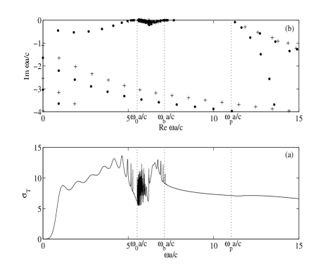
Figure 1: a) Total cross section $\sigma_{T}$. b) Scattering resonances in the complex $\omega a/c$ plane. Dots $(\cdot)$ correspond to poles of $S^{E}(\omega)$ while plus ($+$) correspond to poles of $S^{M}(\omega)$.

II.2 Numerical results and physical interpretation

In Fig. 1a, we display the total cross section plotted as a function of the reduced frequency $\omega a/c$. Rapid variations of sharp characteristic shapes can be observed. Such a strongly fluctuating behavior is due to the scattering resonances associated with the long-lived resonant modes of the sphere, i.e., the long-lived resonant states of the photon-sphere system: when a pole of the $S$ matrix is sufficiently close to the real axis in the complex $\omega$ plane, it has a strong influence on the total cross section. In Fig. 1b, resonances are exhibited for the two polarizations. For certain frequencies, we can clearly observe a one-to-one correspondence between the peaks of $\sigma_{T}(\omega)$ and the resonances near the real $\omega a/c$ axis but, in general, the situation seems very confused. This is due to the profusion of long-lived resonant modes in and around the frequency range where the sphere presents a left-handed behavior. In spite of that, it should be nevertheless noted that (i) the strongly fluctuating behavior generated by electric resonances (TM polarization) is localized within and slightly around the frequency range where the sphere presents a left-handed behavior and (ii) the strongly fluctuating behavior generated by magnetic resonances (TE polarization) is totally localized within that frequency range. Furthermore, by zooming in on the distribution of resonances in regions close to the real axis of the complex $\omega$ plane, we have also observed accumulations of resonances for large values of $\ell$:

(i) For the TM polarization, there exists an accumulation of resonances which converges to the limiting frequency $\omega_{s}$ satisfying

$$\epsilon(\omega_{s})+1=0$$ (15)

and given by

$$\omega_{s}=\frac{\omega_{p}}{\sqrt{2}}.$$ (16)

We have for the corresponding numerical reduced frequency $\omega_{s}a/c\approx 7.806$.

(ii) For the TE polarization, there exists an accumulation of resonances at the limiting frequency $\omega_{f}$ satisfying

$$\mu(\omega_{f})+1=0$$ (17)

and given by

$$\omega_{f}=\omega_{0}\sqrt{\frac{2}{2-F}}.$$ (18)

We have for the corresponding numerical reduced frequency $\omega_{f}a/c\approx 6.172$.

(iii) For both polarizations, there exists an accumulation of resonances at the pole $\omega_{0}$ of $\mu(\omega)$ which corresponds more precisely to

$$\mu(\omega_{0})=-\infty.$$ (19)

From now on, we shall more particularly focus our attention on the physical interpretation of the long-lived resonant modes whose excitation frequencies belong to frequency ranges in which $n(\omega)<0$. We shall prove that the corresponding resonances are generated by exponentially small attenuated SP’s propagating close to the sphere surface and we shall provide a numerical and a theoretical description of these surface waves. The corresponding resonant modes are the so-called RSPM’s. For the other resonant modes associated with bulk polaritons (the resonant modes whose excitation frequencies belong to the frequency range in which $n(\omega)>0$ and those with shorter lifetime), we do not provide a similar analysis. This is not very serious as they do not have, in physics, the importance of RSPM’s. Indeed, in the new field of plasmonics, those are the SP’s with long propagation lengths and therefore very small attenuations that are especially interesting from the point of view of the practical applications. Furthermore, if we consider the photon-sphere system as an artificial atom for which the photon plays the usual role of the electron, we must then keep in mind that, in the scattering of a photon with frequency $\omega^{(o)}_{\ell p}$, a decaying state (i.e., a quasibound state) of the photon-sphere system is formed. It has a finite lifetime proportional to $1/\Gamma_{\ell p}$. The resonant states whose complex frequencies belong to the family generated by SP’s are therefore the most interesting because they are very long-lived states.

We shall finally conclude this section by making a brief comparison with the results obtained in our previous studies concerning the left-handed cylinderAncey et al. (2005) and the metallic and semiconducting spheresAncey et al. (cond-mat/0705.4212):

(i) The total cross sections for the left-handed cylinder and the left-handed sphere as well as their spectra of resonances are rather similar. However, it should be noted that in the scattering by a sphere both the TM and TE polarizations contribute to the total cross section (we recall that for the cylinder, the two polarizations can be studied separately). But, it is also important to note that, for both scatterers, SP’s and their associated RSPM’s correspond to only one polarization (the TE polarization for the cylinder and the TM polarization for the sphere).

(ii) As far as the spectrum of resonances is concerned, the left-handed sphere is a physical system much richer than the metallic or the semiconducting sphere (see Figs. 1 and 2 of Ref. Ancey et al., cond-mat/0705.4212 and the discussion at the end of Sec. II of that reference) and this is certainly very interesting for practical applications of left-handed electromagnetism and more particularly in plasmonics and in cavity quantum electrodynamics.

III Semiclassical analysis: Regge poles, surface polaritons, and resonances

III.1 Complex angular momentum approach: Results

In the CAM approachNewton (1982); Nussenzveig (1992); W. T. Grandy (2000), Regge poles determined by solving Eq. (14) are crucial to describe diffraction as well as resonance phenomena in terms of surface waves. From the Regge trajectories associated with the SP’s supported by the left-handed sphere, i.e., from the curves $\lambda_{\mathrm{SP}}=\lambda_{\mathrm{SP}}(\omega)$ traced out in the CAM plane by the corresponding Regge poles as a function of the frequency, we can more particularly deduce the following:

(i) the dispersion relations of SP’s which connect their wave numbers $k_{\mathrm{SP}}$ with the frequency $\omega$:

$$k_{\mathrm{SP}}(\omega)=\frac{\mathrm{Re}\,\lambda_{\mathrm{SP}}(\omega)}{a},$$ (20)

(ii) the dampings $\mathrm{Im}\,\lambda_{\mathrm{SP}}(\omega)$ of SP’s,

(iii) the phase velocities $v_{p}$ as well as the group velocities $v_{g}$ of SP’s:

$$v_{p}=\frac{a\omega}{\mathrm{Re}\,\lambda_{\mathrm{SP}}(\omega)}\quad\mathrm{and}\quad v_{g}=\frac{d~{}a\omega}{d~{}\mathrm{Re}\,\lambda_{\mathrm{SP}}(\omega)},$$ (21)

(iv) the semiclassical formula (a Bohr-Sommerfeld-type quantization condition) which provides the location of the excitation frequencies $\omega^{(0)}_{\ell\mathrm{SP}}$ of the resonances generated by SP’s:

$$\mathrm{Re}\,\lambda_{\mathrm{SP}}\left(\omega^{(0)}_{\ell\mathrm{SP}}\right)=\ell+1/2,\qquad\ell=1,2,\dots,$$ (22)

(v) the semiclassical formula which provides the widths of these resonances

$$\frac{\Gamma_{\ell\mathrm{SP}}}{2}=\left.\frac{\mathrm{Im}\,\lambda_{\mathrm{SP}}(\omega)[d/d\omega\,\mathrm{Re}\,\lambda_{\mathrm{SP}}(\omega)]}{[d/d\omega\,\mathrm{Re}\,\lambda_{\mathrm{SP}}(\omega)]^{2}+[d/d\omega\,\mathrm{Im}\,\lambda_{\mathrm{SP}}(\omega)]^{2}}\right|_{\omega=\omega^{(0)}_{\ell\mathrm{SP}}}$$ (23)

and which reduces, in the frequency range where the condition $|d/d\omega\,\mathrm{Re}\,\lambda_{\mathrm{SP}}(\omega)|\gg|d/d\omega\,\mathrm{Im}\,\lambda_{\mathrm{SP}}(\omega)|$ is satisfied, to

$$\frac{\Gamma_{\ell\mathrm{SP}}}{2}=\left.\frac{\mathrm{Im}\,\lambda_{\mathrm{SP}}(\omega)}{d/d\omega\,\ \mathrm{Re}\,\lambda_{\mathrm{SP}}(\omega)}\right|_{\omega=\omega^{(0)}_{\ell\mathrm{SP}}}.$$ (24)

All these results can be established by generalizing, mutatis mutandis, our approach and our calculations developed in Refs. Ancey et al., 2004, 2005 for dispersive cylinders. The transition from two dimensions to three dimensions induces some additional technical difficulties (vectorial treatment, existence of a caustic, asymptotics for spherical harmonics, etc.) which can be overcome following and extending the works of Newton in quantum mechanics (see Chap. 13 of Ref. Newton, 1982) and the works of NussenzveigNussenzveig (1992) and GrandyW. T. Grandy (2000) in electromagnetism of ordinary dielectric media.

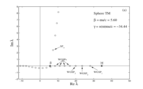
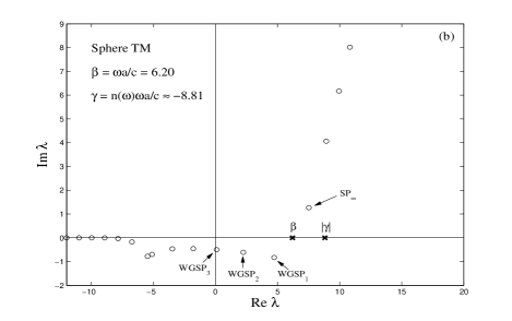
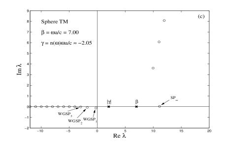
Figure 2: Regge poles in the CAM plane for the TM polarization. a) The distribution corresponds to $\omega a/c=5.6$. b) The distribution corresponds to $\omega a/c=6.2$. c) The distribution corresponds to $\omega a/c=7.0$.

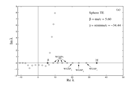
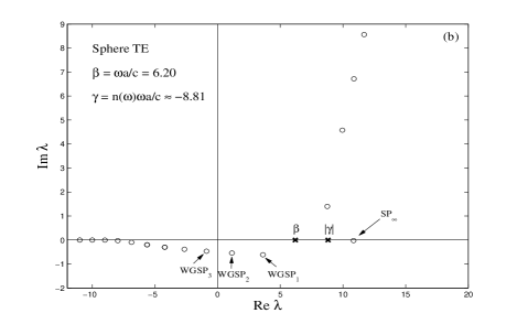
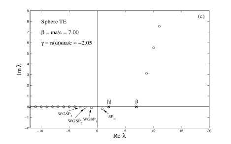
Figure 3: Regge poles in the CAM plane for the TE polarization. a) The distribution corresponds to $\omega a/c=5.6$. b) The distribution corresponds to $\omega a/c=6.2$. c) The distribution corresponds to $\omega a/c=7.0$.

III.2 Regge poles and Regge trajectories

Figures 2 and 3 exhibit the distribution of Regge poles for both polarizations for three different reduced frequencies lying in the frequency region where $n(\omega)<0$. We have identified and indicated some particular Regge poles which are associated with surface waves orbiting around the left-handed sphere and which explain its resonant behavior. These figures are at first sight qualitatively similar to Figs. (4) and (5) of Ref. Ancey et al., 2005 where we displayed the corresponding Regge pole structures for the left-handed cylinder. It should be however noted that, in the transition from the cylinder to the sphere, the TM and TE polarizations are exchanged and curvature corrections induce modifications in the quantitative behavior (as we shall show in Sec. IV). More precisely, for both polarizations, we can observe in Figs. 2 and 3 the following.

– One of these Regge poles is associated with the SP noted ${\mathrm{SP}_{\infty}}$ which, as we shall show in Sec. IV, corresponds in the large radius limit (i.e., for $a\to\infty$) to a SP supported by the plane interface and theoretically described in Refs. Ruppin, 2000b; Darmanyan et al., 2003; Shadrivov et al., 2004.

– The other Regge poles are associated with an infinite family of SP’s of whispering gallery type denoted by ${\mathrm{WGSP}_{n}}$ with $n\in\mathbb{N}^{*}$ which have no analogs for the plane interface (see Sec. IV) as well as for curved metallic or semiconducting interfaces (see Refs. Ancey et al., 2004, cond-mat/0705.4212).

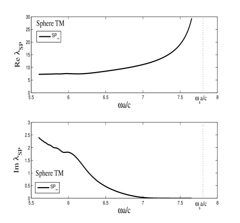
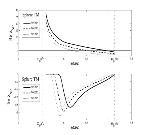
Figure 4: Regge trajectory for the Regge pole associated with ${\mathrm{SP}_{\infty}}$ (TM polarization).

Figure 5: Regge trajectories for the Regge poles associated with the first three whispering-gallery SP’s (TM polarization).

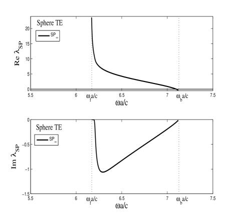
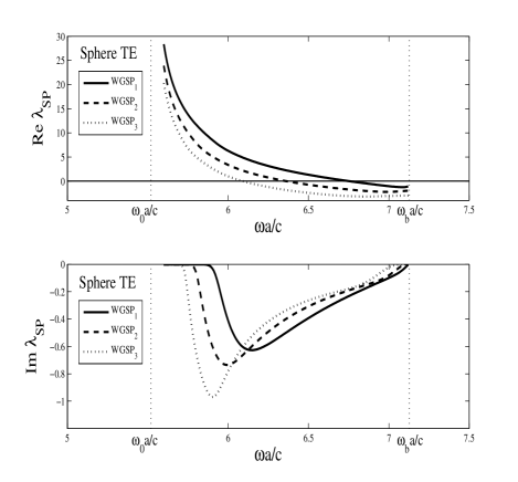
Figure 6: Regge trajectory for the Regge pole associated with ${\mathrm{SP}_{\infty}}$ (TE polarization).

Figure 7: Regge trajectories for the Regge poles associated with the first three whispering-gallery SP’s (TE polarization).

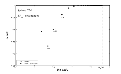
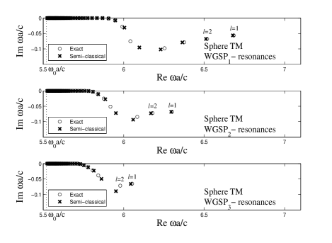
Figure 8: Resonances generated by ${\mathrm{SP}_{\infty}}$ (TM polarization).

Figure 9: Resonances generated by the first three whispering-gallery SP’s (TM polarization).

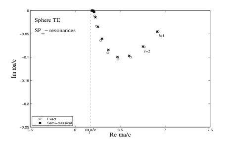
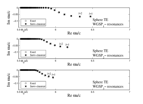
Figure 10: Resonances generated by ${\mathrm{SP}_{\infty}}$ (TE polarization).

Figure 11: Resonances generated by the first three whispering-gallery SP’s (TE polarization).

Figure 12: Zoom-in on the total cross section $\sigma_{T}$.

In Figs. 5-7, we have displayed the Regge trajectories of the first SP’s for the TM and TE polarizations. They have been obtained by solving numerically Eq. (14). We can observe some interesting features:

– The dispersion curve for the surface wave ${\mathrm{SP}_{\infty}}$ of the TM polarization is a positive and monotonically increasing function of $\omega$. As a consequence, the associated group and phase velocities given by Eq. (21) are both positive and ${\mathrm{SP}_{\infty}}$ has an ordinary behavior. It should be also noted that this SP exists in the frequency range $\omega\in]0,\omega_{s}[$ and therefore in the range $]\omega_{0},\omega_{b}[$ where the refraction index is negative but also outside this range. For low values of $\omega$, its damping becomes very large and thus this surface wave has a negligible role for these frequencies in the scattering process and in the resonance mechanism. Furthermore, as $\omega\to\omega_{s}$ the dispersion curve increases indefinitely. This result will permit us to explain the accumulation of resonances which converge to the limiting frequency $\omega_{s}$ for the TM polarization.

– The dispersion curve for the surface wave ${\mathrm{SP}_{\infty}}$ of the TE polarization is a positive and monotonically decreasing function of $\omega$. As a consequence, the associated phase velocity is positive while the group velocity is negative [see Eq. (21)]. ${\mathrm{SP}_{\infty}}$ has a “left-handed behavior”. It should be also noted that this SP only exists in the frequency range $]\omega_{f},\omega_{b}[$ which is included in the frequency range $]\omega_{0},\omega_{b}[$ where the refraction index is negative. Its damping is always weak and thus this surface wave always plays a significant role in the scattering process and in the resonance mechanism. Finally, as $\omega\to\omega_{f}$ the dispersion curve increases indefinitely. This result will permit us to explain the accumulation of resonances which converge to the limiting frequency $\omega_{f}$ for the TE polarization.

– As far as the surface waves ${\mathrm{WGSP}_{n}}$ ($n\in\mathbb{N}^{*}$) of the TM and TE polarizations are concerned, they present, at first sight, a behavior which is rather independent of the polarization. The real part of a given Regge pole $\lambda_{\mathrm{WGSP}_{n}}$ vanishes for a frequency in the range $]\omega_{0},\omega_{b}[$ and becomes negative. This Regge pole then migrates to the third quadrant of the CAM plane and becomes unphysical. So we can consider that the surface waves ${\mathrm{WGSP}_{n}}$ with $n\in\mathbb{N}^{*}$ only exist in a subdomain of the frequency range $]\omega_{0},\omega_{b}[$ where the refraction index is negative. The dispersion relations of all these surface waves are positive but monotonically decreasing functions. Their group velocities are always negative while their phase velocities are positive [see Eq. (21)]. All these SP’s thus have a left-handed behavior. Furthermore, because the dampings of these surface waves are always weak, they all play a significant role in the scattering process and in the resonance mechanism. Finally, it should be noted that as $\omega\to\omega_{0}$, the dispersion curves increase indefinitely. This result will permit us to explain the accumulation of resonances which converges to the limiting frequency $\omega_{0}$ for the TM and TE polarizations.

III.3 Resonances

In Figs. 9-11 we present samples of complex frequencies for the RSPM’s associated with the surface waves ${\mathrm{SP}_{\infty}}$ and ${\mathrm{WGSP}_{n}}$ with $n=1$, $2$ and $3$. They have been calculated from the semiclassical formulas (22) and (23) by using the Regge trajectories determined numerically by solving Eq. (14) (see Figs. 5-7). A comparison between the semiclassical spectra and the “exact ones” (calculated by solving numerically Eq. 12) shows a very good agreement. Moreover, we can also observe some interesting features (mutatis mutandis they were already present for the left-handed cylinder):

– The resonance spectrum associated with the surface wave ${\mathrm{SP}_{\infty}}$ of the TM polarization (see Fig. 9) extends beyond the frequency range $]\omega_{0},\omega_{b}[$ where the sphere presents a left-handed behavior because ${\mathrm{SP}_{\infty}}$ exists for $\omega\in]0,\omega_{s}[$. Furthermore, inserted into the semiclassical formulas (22) and (23), the behavior of the Regge trajectory of $\lambda_{\mathrm{SP}_{\infty}}$ near $\omega_{s}$ easily explains the existence of the family of resonances close to the real axis of the complex $\omega$ plane which converges for large $\ell$ to the limiting frequency $\omega_{s}$.

– The resonance spectrum associated with the surface wave ${\mathrm{SP}_{\infty}}$ of the TE polarization (see Fig. 11) fully lies inside the frequency range $]\omega_{0},\omega_{b}[$ where the sphere presents a left-handed behavior because ${\mathrm{SP}_{\infty}}$ exists only in that range. Furthermore, inserted into the semiclassical formulas (22) and (23), the behavior of the Regge trajectory of $\lambda_{\mathrm{SP}_{\infty}}$ near $\omega_{f}$ explains the existence of the family of resonances close to the real axis of the complex $\omega$ plane which converges for large $\ell$ to the limiting frequency $\omega_{f}$.

– The resonance spectra associated with the surface waves ${\mathrm{WGSP}_{n}}$ ($n\in\mathbb{N}^{*}$) of the TM and TE polarizations (see Figs. 9 and 11) fully lie inside the frequency range $]\omega_{0},\omega_{b}[$ where the sphere presents a left-handed behavior because all these surface waves exist only in that range. Furthermore, inserted into the semiclassical formulas (22) and (23), the behavior of the Regge trajectory of a given Regge pole $\lambda_{\mathrm{WGSP}_{n}}$ near $\omega_{0}$ explains the existence of a corresponding family of resonances close to the real axis of the complex $\omega$ plane which converges for large $\ell$ to the limiting frequency $\omega_{0}$.

In conclusion, we have established a connection between the complex frequencies of the long-lived resonant modes (or RSPM’s) of the left-handed sphere and the SP’s noted ${\mathrm{SP}_{\infty}}$ and ${\mathrm{WGSP}_{n}}$ with $n\in\mathbb{N}^{*}$ which are supported by its surface. In other words, in spite of the great confusion which seems to prevail in the resonance spectrum of the left-handed sphere (see Sec. II), we have been able to fully classify and physically interpret the resonances thanks to CAM techniques. We now invite the reader to look at Fig. 12 where we have zoomed in on Fig. 1. On the total cross sections $\sigma_{T}(\omega)$ we have identified the peaks corresponding to resonances and, for each one, we have specified the SP which has generated it as well as its polarization and the associated “quantum number” $\ell$. This has been achieved by using the results displayed on Figs. 9-11. It is also possible to identify the “quantum numbers” of the different resonant modes by plotting the associated distribution of electromagnetic energy density. Indeed, the number of local maxima is twice the quantum number $\ell$. These distributions can been obtained from the theory developed in Refs. Ruppin, 1998, 2002. For example, in Figs. 13-16 we have displayed, for the TE polarization, the energy distributions for the resonant modes $\ell=9$ and $\ell=10$ generated by ${\mathrm{SP}_{\infty}}$ and for the resonant modes $\ell=8$ and $\ell=9$ generated by ${\mathrm{WGSP}_{1}}$. For obvious symmetry reasons, we have only considered one quarter of the equatorial section of the sphere.

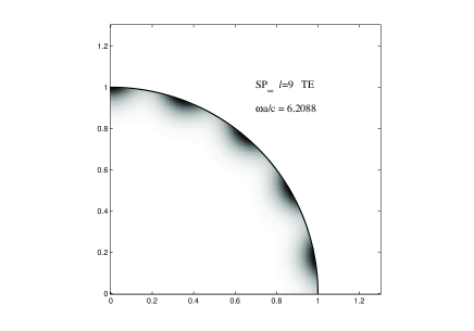
Figure 13: Electromagnetic energy density for the resonant mode $\ell=9$ generated by ${\mathrm{SP}_{\infty}}$ (TE polarization).

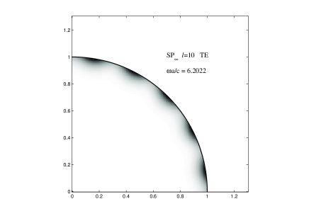
Figure 14: Electromagnetic energy density for the resonant mode $\ell=10$ generated by ${\mathrm{SP}_{\infty}}$ (TE polarization).

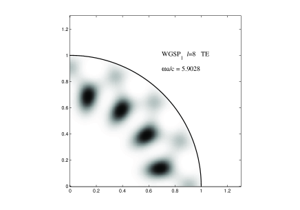
Figure 15: Electromagnetic energy density for the resonant mode $\ell=8$ generated by ${\mathrm{WGSP}_{1}}$ (TE polarization).

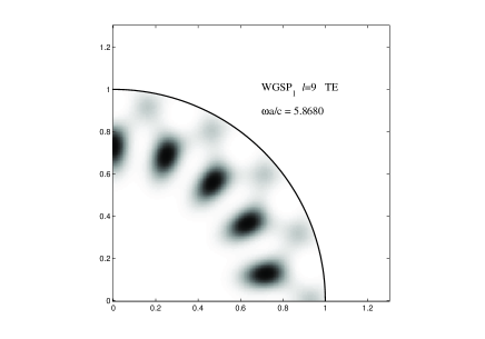
Figure 16: Electromagnetic energy density for the resonant mode $\ell=9$ generated by ${\mathrm{WGSP}_{1}}$ (TE polarization).

IV Asymptotics for surface polaritons and physical description

In order to obtain a deeper physical understanding of the SP’s orbiting around the left-handed sphere and to justify the terminology previously used (i.e., the notations ${\mathrm{SP}_{\infty}}$ and ${\mathrm{WGSP}_{n}}$ for the SP’s), we must “analytically” solve Eq. (14) for $\lambda=\lambda_{\mathrm{SP}}$ or equivalently

$$\sqrt{\frac{\epsilon(\omega)}{\mu(\omega)}}\frac{\zeta_{\lambda_{\mathrm{SP}}-1/2}^{(1)^{\prime}}\left(a\omega/c\right)}{\zeta_{\lambda_{\mathrm{SP}}-1/2}^{(1)}\left(a\omega/c\right)}=\frac{\psi_{\lambda_{\mathrm{SP}}-1/2}^{\prime}\left[n(\omega)a\omega/c\right]}{\psi_{\lambda_{\mathrm{SP}}-1/2}\left[n(\omega)a\omega/c\right]}$$ (25)

for the TM polarization and

$$\sqrt{\frac{\mu(\omega)}{\epsilon(\omega)}}\frac{\zeta_{\lambda_{\mathrm{SP}}-1/2}^{(1)^{\prime}}\left(a\omega/c\right)}{\zeta_{\lambda_{\mathrm{SP}}-1/2}^{(1)}\left(a\omega/c\right)}=\frac{\psi_{\lambda_{\mathrm{SP}}-1/2}^{\prime}\left[n(\omega)a\omega/c\right]}{\psi_{\lambda_{\mathrm{SP}}-1/2}\left[n(\omega)a\omega/c\right]}$$ (26)

for the TE polarization. In other words, we seek to obtain explicit formulas for the Regge poles of the problem. We have previously done it for metallic and semiconducting objectsAncey et al. (2004, cond-mat/0705.4212) as well as for left-handed cylindersAncey et al. (2005) and we shall here extend such an analysis to left-handed spheres. We were recently aware of a beautiful article by BerryBerry (1975) where this problem has also been considered for a curved dielectric interface with an electric permittivity negative and independent of $\omega$.

By replacing Ricatti-Bessel functions by spherical Bessel functions and then using their relations with the ordinary Bessel functions (see Ref. Abramowitz and Stegun, 1965)

$$j_{\lambda}(z)=\sqrt{\frac{\pi}{2z}}J_{\lambda+1/2}(z)\quad\mathrm{and}\quad h^{(1)}_{\lambda}(z)=\sqrt{\frac{\pi}{2z}}H^{(1)}_{\lambda+1/2}(z),$$ (27)

as well as $J_{\lambda}(-z)=e^{i\pi\lambda}J_{\lambda}(z)$ and $J^{\prime}_{\lambda}(-z)=-e^{i\pi\lambda}J^{\prime}_{\lambda}(z)$ (see Ref. Abramowitz and Stegun, 1965) in order to take into account that $n(\omega)<0$ in the most interesting frequency range, it is easy to prove that Eqs. (25) and (26) respectively reduce to

$$-\frac{J^{\prime}_{\lambda_{\mathrm{SP}}}[|n(\omega)|\,\omega a/c]}{J_{\lambda_{\mathrm{SP}}}[|n(\omega)|\,\omega a/c]}+\frac{1}{2n(\omega)}\left(\frac{c}{\omega a}\right)$$

$$\qquad=\sqrt{\frac{\epsilon(\omega)}{\mu(\omega)}}\frac{H_{\lambda_{\mathrm{SP}}}^{(1)^{\prime}}(\omega a/c)}{H_{\lambda_{\mathrm{SP}}}^{(1)}(\omega a/c)}+\frac{1}{2}\sqrt{\frac{\epsilon(\omega)}{\mu(\omega)}}\left(\frac{c}{\omega a}\right)$$ (28)

for the TM polarization and

$$-\frac{J^{\prime}_{\lambda_{\mathrm{SP}}}[|n(\omega)|\,\omega a/c]}{J_{\lambda_{\mathrm{SP}}}[|n(\omega)|\,\omega a/c]}+\frac{1}{2n(\omega)}\left(\frac{c}{\omega a}\right)$$

$$\qquad=\sqrt{\frac{\mu(\omega)}{\epsilon(\omega)}}\frac{H_{\lambda_{\mathrm{SP}}}^{(1)^{\prime}}(\omega a/c)}{H_{\lambda_{\mathrm{SP}}}^{(1)}(\omega a/c)}+\frac{1}{2}\sqrt{\frac{\mu(\omega)}{\epsilon(\omega)}}\left(\frac{c}{\omega a}\right)$$ (29)

for the TE polarization. These two last equations must be compared respectively with Eqs. (37) and (38) of Ref. Ancey et al., 2005 which provide SP Regge poles for the left-handed cylinder. The first term on the left-hand side and on the right-hand side of Eqs. (IV) and (IV) are exactly those appearing in Eqs. (37) and (38) of Ref. Ancey et al., 2005. The remaining terms are curvature corrections due to the change of dimension. Equations (IV) and (IV) can be solved following the method used in order to solve Eqs. (37) and (38) of Ref. Ancey et al., 2005, i.e., by using asymptotic analysis. As we have previously noted in Ref. Ancey et al., 2005, the choice of the asymptotic expansions for the Bessel functions strongly depends on the relative positions of the arguments $|n(\omega)|\omega a/c$ and $\omega a/c$ with respect to the complex order $\lambda_{\mathrm{SP}}$. In order to simplify the discussion, we choose to describe theoretically SP’s in the frequency ranges where they generate the RSPM’s with the longest lifetime (such modes are the most important from the physical point of view). In other words, we shall seek $\lambda_{\mathrm{SP}_{\infty}}(\omega)$ for the TM polarization with $\omega$ in the neighborhood of $\omega_{s}$, $\lambda_{\mathrm{SP}_{\infty}}(\omega)$ for the TE polarization with $\omega$ in the neighborhood of $\omega_{f}$ and $\lambda_{\mathrm{WGSP}_{n}}(\omega)$ for both polarizations with $\omega$ in the neighborhood of $\omega_{0}$ . In fact, in spite of these restrictions, we shall obtain asymptotic results valid in large frequency ranges.

IV.1 Asymptotics for surface polaritons of ${\mathrm{SP}_{\infty}}$-type and physical description

Let us first consider the Regge pole associated with ${\mathrm{SP}_{\infty}}$ for the TM polarization. We assume $\omega$ in the neighborhood of $\omega_{s}$ [but also that $\omega<\omega_{b}$ so that $n(\omega)<0$] and then we can also assume that $\mathrm{Re}\,\lambda_{\mathrm{SP}_{\infty}}(\omega)>\omega a/c>|n(\omega)|\omega a/c$ and formally that $\mathrm{Re}\,\lambda_{\mathrm{SP}_{\infty}}(\omega)\gg 1$ and $\mathrm{Re}\,\lambda_{\mathrm{SP}_{\infty}}(\omega)\gg\mathrm{Im}\,\lambda_{\mathrm{SP}_{\infty}}(\omega)$. As a consequence, we can use the Debye asymptotic expansions for $J_{\lambda}(z)$ and $H_{\lambda}^{(1)}(z)$ valid for large orders (see our previous paperAncey et al. (2005) for details as well as Appendix A of Ref. Nussenzveig, 1965 or Ref. Watson, 1995). We can then write

$$\frac{J^{\prime}_{\lambda_{\mathrm{SP}_{\infty}}}[|n(\omega)|\omega a/c]}{J_{\lambda_{\mathrm{SP}_{\infty}}}[|n(\omega)|\omega a/c]}\sim\frac{\left[\lambda_{\mathrm{SP}_{\infty}}^{2}-(|n(\omega)|\omega a/c)^{2}\right]^{1/2}}{|n(\omega)|(\omega a/c)}$$ (30)

and

$$\frac{H_{\lambda_{\mathrm{SP}_{\infty}}}^{(1)^{\prime}}(\omega a/c)}{H_{\lambda_{\mathrm{SP}_{\infty}}}^{(1)}(\omega a/c)}\sim-\frac{\left[\lambda_{\mathrm{SP}_{\infty}}^{2}-(\omega a/c)^{2}\right]^{1/2}}{(\omega a/c)}$$

$$\qquad\times\left(1-ie^{2\alpha(\lambda_{\mathrm{SP}_{\infty}},\omega a/c)}\right)$$ (31)

where

$$\alpha(\lambda,z)=(\lambda^{2}-z^{2})^{1/2}-\lambda\,\ln\left(\frac{\lambda+(\lambda^{2}-z^{2})^{1/2}}{z}\right).$$ (32)

In Eq. (IV.1), we have taken into account an exponentially small contribution (the term $\exp[2\alpha(\lambda_{\mathrm{SP}_{\infty}},\omega a/c)]$) which lies beyond all orders in perturbation theory. This term can be captured by carefully taking into account Stokes phenomenon and is necessary to extract the asymptotic expression of the imaginary part of $\lambda_{\mathrm{SP}}$. [In Eq. (IV.1) we have given to the Stokes multiplier function the value $1/2$.] For more precision, we refer to our previous paperAncey et al. (2005) as well as to Refs. Berry, 1989; Dingle, 1973; Segur et al., 1991; Berry and Howls, 1990. Now, by inserting (30) and (IV.1) into Eq. (IV), we obtain an equation which can be “easily” solved. We first neglect the exponentially small term and this equation reduces to a fourth-order polynomial equation. We only retain the physical solution which correctly modifies the formula (47a) obtained in Ref. Ancey et al., 2005 for the corresponding SP of the left-handed cylinder. It provides the real part of $\lambda_{\mathrm{SP}_{\infty}}(\omega)$. We then take into account the exponentially small term and we obtain perturbatively the imaginary part of $\lambda_{\mathrm{SP}_{\infty}}(\omega)$. We finally have

$$\mathrm{Re}\,\lambda_{\mathrm{SP}_{\infty}}(\omega)\sim\left(\frac{\omega a}{c}\right)\times$$

$$\sqrt{\frac{|\epsilon(\omega)|[|\epsilon(\omega)|+\mu(\omega)]}{\epsilon^{2}(\omega)-1}+\frac{\epsilon^{2}(\omega)+1}{4[1-|\epsilon(\omega)|]^{2}}\left(\frac{c}{\omega a}\right)^{2}+\sqrt{\frac{\epsilon^{2}(\omega)[|\epsilon(\omega)|\mu(\omega)+1]}{[\epsilon^{2}(\omega)-1][1-|\epsilon(\omega)|]^{2}}\left(\frac{c}{\omega a}\right)^{2}+\frac{\epsilon^{2}(\omega)}{4[1-|\epsilon(\omega)|]^{4}}\left(\frac{c}{\omega a}\right)^{4}}}$$

(33a)

$$\mathrm{Im}\,\lambda_{\mathrm{SP}_{\infty}}(\omega)\sim\left(\frac{\epsilon^{2}(\omega)}{\epsilon^{2}(\omega)-1}\right)\times\frac{\left(\mathrm{Re}\,\lambda_{\mathrm{SP}_{\infty}}(\omega)\right)^{2}-\left({\omega a/c}\right)^{2}}{\mathrm{Re}\,\lambda_{\mathrm{SP}_{\infty}}(\omega)}\times\exp[2\alpha(\mathrm{Re}\,\lambda_{\mathrm{SP}_{\infty}}(\omega),\omega a/c)].$$ (33b)

Let us now consider the Regge pole associated with ${\mathrm{SP}_{\infty}}$ of the TE polarization. In order to describe it, we must solve Eq. (IV) which only differs from Eq. (IV) by the exchange of $\epsilon(\omega)$ and $\mu(\omega)$. Here, we assume $\omega$ in the neighborhood of $\omega_{f}$ and then we can also assume that $\mathrm{Re}\,\lambda_{\mathrm{SP}_{\infty}}(\omega)>|n(\omega)|\omega a/c>\omega a/c$ and formally that $\mathrm{Re}\,\lambda_{\mathrm{SP}_{\infty}}(\omega)\gg 1$ and $\mathrm{Re}\,\lambda_{\mathrm{SP}_{\infty}}(\omega)\gg\mathrm{Im}\,\lambda_{\mathrm{SP}_{\infty}}(\omega)$. As a consequence, we can use again the Debye asymptotic expansions for $J_{\lambda}(z)$ and $H_{\lambda}^{(1)}(z)$ valid for large orders and the resolution of Eq. (IV) can be modeled on that of Eq. (IV). Formulas (30) and (IV.1) remain valid and by inserting them into Eq. (IV), we obtain

$$\mathrm{Re}\,\lambda_{\mathrm{SP}_{\infty}}(\omega)\sim\left(\frac{\omega a}{c}\right)\times$$

$$\sqrt{\frac{|\mu(\omega)|[|\mu(\omega)|+\epsilon(\omega)]}{\mu^{2}(\omega)-1}+\frac{\mu^{2}(\omega)+1}{4[1-|\mu(\omega)|]^{2}}\left(\frac{c}{\omega a}\right)^{2}-\sqrt{\frac{\mu^{2}(\omega)[|\mu(\omega)|\epsilon(\omega)+1]}{[\mu^{2}(\omega)-1][1-|\mu(\omega)|]^{2}}\left(\frac{c}{\omega a}\right)^{2}+\frac{\mu^{2}(\omega)}{4[1-|\mu(\omega)|]^{4}}\left(\frac{c}{\omega a}\right)^{4}}}$$

(34a)

$$\mathrm{Im}\,\lambda_{\mathrm{SP}_{\infty}}(\omega)\sim\left(\frac{\mu^{2}(\omega)}{\mu^{2}(\omega)-1}\right)\times\frac{\left(\mathrm{Re}\,\lambda_{\mathrm{SP}_{\infty}}(\omega)\right)^{2}-\left({\omega a/c}\right)^{2}}{\mathrm{Re}\,\lambda_{\mathrm{SP}_{\infty}}(\omega)}\times\exp[2\alpha(\mathrm{Re}\,\lambda_{\mathrm{SP}_{\infty}}(\omega),\omega a/c)].$$ (34b)

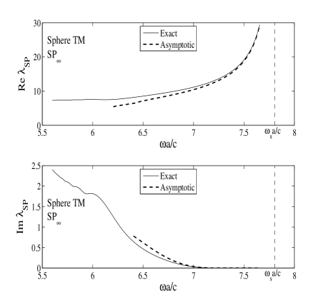
Figure 17: Regge trajectory for the Regge pole associated with ${\mathrm{SP}_{\infty}}$ (TM polarization). Comparison between exact and asymptotic theories.

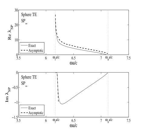
Figure 18: Regge trajectory for the Regge pole associated with ${\mathrm{SP}_{\infty}}$ (TE polarization). Comparison between exact and asymptotic theories.

Equations (33a)-(33b) and (34a)-(34b) provide respectively analytic expressions for the dispersion relation and the damping of the surface polaritons ${\mathrm{SP}_{\infty}}$ of the TM and TE polarizations. The following important physical features must be noted:

– These two SP’s present exponentially small attenuations.

– Their wave numbers $k_{\mathrm{SP}_{\infty}}(\omega)$ can be obtained from (33a) and (20) for the TM polarization and from (34a) and (20) for the TE polarization and they could permit us to derive analytically their phase velocity $v_{p}=\omega/k_{\mathrm{SP}_{\infty}}(\omega)$ as well as their group velocity $v_{g}=d\omega/dk_{\mathrm{SP}_{\infty}}(\omega)$.

– For $a\to\infty$ – i.e., in the flat interface limit – the wave number $k_{\mathrm{SP}_{\infty}}(\omega)$ for the TM polarization reduces to

$$k_{\mathrm{SP}_{\infty}}(\omega)\sim\left(\frac{\omega}{c}\right)\sqrt{\frac{|\epsilon(\omega)|[|\epsilon(\omega)|+\mu(\omega)]}{\epsilon^{2}(\omega)-1}}.$$ (35)

This expression is the usual dispersion relation found in Refs. Ruppin, 2000b; Darmanyan et al., 2003; Shadrivov et al., 2004 for the $p$-polarized SP - i.e., the SP for which the magnetic field $\mathbf{H}$ is normal to the incidence plane - supported by the flat interface. For the TM polarization, ${\mathrm{SP}_{\infty}}$ is therefore the counterpart of the $p$-polarized SP supported by the flat interface.

– For $a\to\infty$ – i.e., in the flat interface limit – the wave number $k_{\mathrm{SP}_{\infty}}(\omega)$ for the TE polarization reduces to

$$k_{\mathrm{SP}_{\infty}}(\omega)\sim\left(\frac{\omega}{c}\right)\sqrt{\frac{|\mu(\omega)|[|\mu(\omega)|+\epsilon(\omega)]}{\mu^{2}(\omega)-1}}.$$ (36)

This expression is the usual dispersion relation found in Refs. Ruppin, 2000b; Darmanyan et al., 2003; Shadrivov et al., 2004 for the $s$-polarized SP - i.e., the SP for which the electric field $\mathbf{E}$ is normal to the incidence plane - supported by the flat interface. For the TE polarization, ${\mathrm{SP}_{\infty}}$ is therefore the counterpart of the $s$-polarized SP supported by the flat interface.

– Furthermore, for $a\to\infty$, the imaginary parts (33b) and (34b) of $\lambda_{\mathrm{SP}_{\infty}}$ vanish. In the flat interface limit, $\mathrm{SP}_{\infty}$ for both polarizations have no damping like the SP’s supported by the flat interfaceRuppin (2000b); Darmanyan et al. (2003); Shadrivov et al. (2004).

– A connection with the results obtained in our previous study concerning the left-handed cylinderAncey et al. (2005) can be established. By comparing (33a) with (47a) of Ref. Ancey et al., 2005 and (34a) with (49a) of Ref. Ancey et al., 2005 we can notice that ${\mathrm{SP}_{\infty}}$ of the sphere for the TM (TE) polarization is the counterpart of ${\mathrm{SP}_{\infty}}$ of the cylinder for the TE (TM) polarization. In Eqs. (33a) and (34a), the supplementary terms are associated with the curvature corrections appearing in Eqs. (IV) and (IV). In certain frequency ranges, these corrections are of the same magnitude than the remaining terms. As a consequence, it is not possible to obtain dispersion relations on the sphere perturbatively from those on the cylinder.

– The function $\mathrm{Re}\,\lambda_{\mathrm{SP}_{\infty}}(\omega)$ given by (33a) has a pole when $\epsilon(\omega)+1=0$ – i.e., for $\omega=\omega_{s}$. Furthermore, the imaginary part (33b) of $\lambda_{\mathrm{SP}_{\infty}}$ vanishes for $\omega=\omega_{s}$. These two results explain semiclassically, for the TM polarization, the accumulation of resonances which converge to the limiting frequency $\omega_{s}$.

– The function $\mathrm{Re}\,\lambda_{\mathrm{SP}_{\infty}}(\omega)$ given by (34a) has a pole when $\mu(\omega)+1=0$ – i.e., for $\omega=\omega_{f}$. Furthermore, the imaginary part (34b) of $\lambda_{\mathrm{SP}_{\infty}}$ vanishes for $\omega=\omega_{f}$. These two results explain semiclassically, for the TE polarization, the accumulation of resonances which converge to the limiting frequency $\omega_{f}$.

– We have numerically tested formulas (33a) and (33b) (see Fig. 17) as well as formulas (34a) and (34b) (see Fig. 18). They provide rather good approximations i) for $\mathrm{Re}\,\lambda_{\mathrm{SP}_{\infty}}(\omega)$ in large frequency ranges for both polarizations, ii) for $\mathrm{Im}\,\lambda_{\mathrm{SP}_{\infty}}(\omega)$ in the neighborhood of $\omega_{s}$ for the TM polarization and iii) for $\mathrm{Im}\,\lambda_{\mathrm{SP}_{\infty}}(\omega)$ in the neighborhood of $\omega_{f}$ for the TE polarization.

IV.2 Asymptotics for surface polaritons of ${\mathrm{WGSP}_{n}}$ type and physical description

Let us finally consider the Regge poles associated with the surface waves ${\mathrm{WGSP}_{n}}$ for the TM and TE polarizations. We must now solve Eqs. (IV) and (IV) for $\lambda_{\mathrm{SP}}=\lambda_{\mathrm{WGSP}_{n}}$ by assuming $\omega$ in the neighborhood of $\omega_{0}$. The configuration is identical to that of Ref. Ancey et al., 2005 for the left-handed cylinder. We can consider that $\mathrm{Re}\,\lambda_{\mathrm{WGSP}_{n}}(\omega)>\omega a/c$ and formally that $\mathrm{Re}\,\lambda_{\mathrm{WGSP}_{n}}(\omega)\gg 1$ and $\mathrm{Re}\,\lambda_{\mathrm{WGSP}_{n}}(\omega)\gg\mathrm{Im}\,\lambda_{\mathrm{WGSP}_{n}}(\omega)$. Furthermore, $\lambda_{\mathrm{WGSP}_{n}}$ is in the immediate neighborhood of $|n(\omega)|\omega a/c$ i.e., lies in the Airy circle centered on $|n(\omega)|\omega a/c$. As a consequence, we can still replace $H^{(1)}_{\lambda}(z)$ by its Debye asymptotic expansion valid for large orders and therefore insert (IV.1) into (IV) and (IV). As far as $J_{\lambda}(z)$ is concerned, we must now use its uniform asymptotic expansion (see Appendix A of Ref. Nussenzveig, 1965 or Ref. Watson, 1995)

$$J_{\lambda}(z){\sim}\left(2/z\right)^{1/3}Ai\left[\left(2/z\right)^{1/3}(\lambda-z)\right]$$ (37)

where $Ai(z)$ denotes the Airy functionAbramowitz and Stegun (1965). Thus, we must insert

$$\frac{J_{\lambda_{\mathrm{WGSP}_{n}}}^{{}^{\prime}}[|n(\omega)|\omega a/c]}{J_{\lambda_{\mathrm{WGSP}_{n}}}[|n(\omega)|\omega a/c]}\sim\{{2/[|n(\omega)|\omega a/c]\}}^{1/3}$$

$$\times\frac{{Ai}^{{}^{\prime}}\left[\{{2/[|n(\omega)|\omega a/c]\}}^{1/3}[\lambda_{\mathrm{WGSP}_{n}}-|n(\omega)|\omega a/c]\right]}{Ai\left[\{{2/[|n(\omega)|\omega a/c]\}}^{1/3}[\lambda_{\mathrm{WGSP}_{n}}-|n(\omega)|\omega a/c]\right]}.$$

into (IV) and (IV). We obtain two equations which can be solved by using the method already considered in our previous workAncey et al. (2005) and which is an adaptation of the method invented by Rayleigh a long time ago in order to describe mathematically the whispering-gallery phenomenon in acoustics Rayleigh (1976, 1910) (see also Ref. Streifer and Kodis, 1964). After having noticed that the curvature corrections can be neglected in that configuration, we recover the formulas obtained for the left-handed cylinder. We have

$$\mathrm{Re}\,\lambda_{\mathrm{WGSP}_{n}}(\omega)\sim|n(\omega)|\omega a/c+\left(\frac{|n(\omega)|\omega a/c}{2}\right)^{1/3}x_{n}$$

(39a)

$$\mathrm{Im}\,\lambda_{\mathrm{WGSP}_{n}}(\omega)\sim\sqrt{\frac{\epsilon(\omega)}{\mu(\omega)}}\left(\frac{|n(\omega)|~{}\omega a/c}{2}\right)^{2/3}$$

$$\qquad\qquad\times\frac{\left[\left[\mathrm{Re}\,\lambda_{\mathrm{WGSP}_{n}}(\omega)\right]^{2}-\left({\omega a/c}\right)^{2}\right]^{1/2}}{\left({\omega a/c}\right)x_{n}}$$

$$\qquad\qquad\times\exp\left[2\alpha(\mathrm{Re}\,\lambda_{\mathrm{WGSP}_{n}}(\omega),\omega a/c)\right]$$ (39b)

for the TM polarization and

$$\mathrm{Re}\,\lambda_{\mathrm{WGSP}_{n}}(\omega)\sim|n(\omega)|\omega a/c+\left(\frac{|n(\omega)|\omega a/c}{2}\right)^{1/3}x_{n}$$

(40a)

$$\mathrm{Im}\,\lambda_{\mathrm{WGSP}_{n}}(\omega)\sim\sqrt{\frac{\mu(\omega)}{\epsilon(\omega)}}\left(\frac{|n(\omega)|~{}\omega a/c}{2}\right)^{2/3}$$

$$\qquad\qquad\times\frac{\left[\left[\mathrm{Re}\,\lambda_{\mathrm{WGSP}_{n}}(\omega)\right]^{2}-\left({\omega a/c}\right)^{2}\right]^{1/2}}{\left({\omega a/c}\right)x_{n}}$$

$$\qquad\qquad\times\exp\left[2\alpha(\mathrm{Re}\,\lambda_{\mathrm{WGSP}_{n}}(\omega),\omega a/c)\right]$$ (40b)

for the TE polarization. In Eqs. (39a)-(40b), we have introduced the zeros $x_{n}$ of the Airy function (the first three ones are $x_{1}\approx-2.3381...$, $x_{2}\approx-4.0879...$ and $x_{3}\approx-5.5205...$).

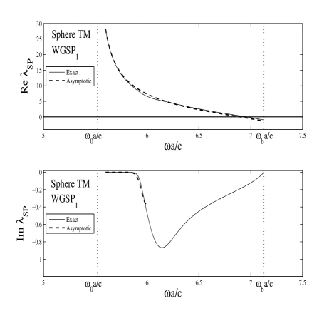
Figure 19: Regge trajectory for the Regge pole associated with ${\mathrm{WGSP}_{1}}$ (TM polarization). Comparison between exact and asymptotic theories.

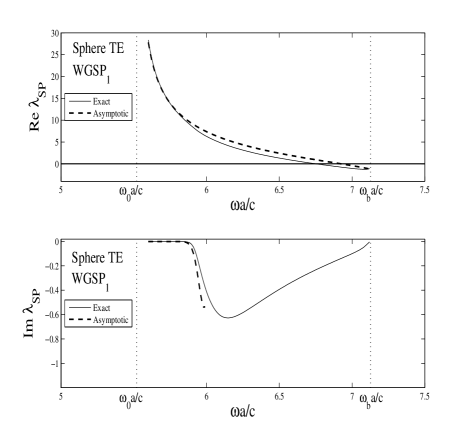
Figure 20: Regge trajectory for the Regge pole associated with ${\mathrm{WGSP}_{1}}$ (TE polarization). Comparison between exact and asymptotic theories.

Equations (39a)-(40b) provide analytic expressions for the dispersion relation and the damping of the surface polaritons ${\mathrm{WGSP}_{n}}$ for both polarizations. These expressions are those already obtained for the left-handed cylinder with the polarizations exchanged: (39a) and (39b) must be compared with (55a) and (55b) of Ref. Ancey et al., 2005 while (40a) and (40b) must be compared with (55a) and (55c) of Ref. Ancey et al., 2005. Therefore, mutatis mutandis, the physical remarks and analysis of Ref. Ancey et al., 2005 concerning the whispering-gallery surface waves propagating on the cylinder can be taken again. We just note that:

– These SP’s have no counterparts in the plane interface case.

– They do not exist for curved metallic or semiconducting interfaces (see Refs. Ancey et al., 2004, cond-mat/0705.4212).

– The function $\mathrm{Re}\,\lambda_{\mathrm{WGSP}_{n}}(\omega)$ given by (39a) or (40a) has a pole which is that of $n(\omega)$ and therefore which corresponds to $\omega=\omega_{0}$. Furthermore, the imaginary parts (39b) and (40b) of $\lambda_{\mathrm{WGSP}_{n}}$ vanish for $\omega=\omega_{0}$. These results justify all our previous remarks concerning the accumulations of resonances which converge to the limiting frequency $\omega_{0}$.

– We have numerically tested formulas (39a)-(40b) (see Figs. 19 and 20 for $\mathrm{WGSP}_{1}$). They provide very good approximations for $\mathrm{Re}\,\lambda_{\mathrm{WGSP}_{1}}(\omega)$ in the full frequency range $]\omega_{0},\omega_{b}[$ where the sphere presents a left-handed behavior. They also provide very good approximations for $\mathrm{Im}\,\lambda_{\mathrm{WGSP}_{1}}(\omega)$ in a rather large frequency range above the limiting frequency $\omega_{0}$.

V Conclusion and perspectives

In the present paper, we have considered the interaction of electromagnetic waves with a sphere fabricated from a left-handed material. We have mainly emphasized the resonant aspects of the problem. We have shown that the long-lived resonant modes can be classified into distinct families, each family being generated by one SP and we have physically described all the SP’s orbiting around the sphere by providing, for each one, a numerical and a semiclassical description of its dispersion relation and its damping.

We have more particularly shown that the left-handed spherical interface can support both TE and TM polarized SP’s. For each polarization, there exists a particular SP which corresponds, in the large radius limit, to the SP which is supported by the plane interface and which has been theoretically described in Refs. Ruppin, 2000b; Darmanyan et al., 2003; Shadrivov et al., 2004. However, there also exists, for each polarization, an infinite family of SP’s of whispering gallery type and these have no analogues in the plane interface case. They are only supported by the curved left-handed interface (they do not exist for curved metallic or semiconducting interfacesAncey et al. (2004, cond-mat/0705.4212)) and they are analogs to those described for the cylindrical interface in Ref. Ancey et al., 2005.

One could believe at first sight that the existence of surface waves of whispering gallery type (and of the associated resonant modes) in the frequency region where both permittivity and permeability of the sphere are negative is rather trivial because they are also present for an ordinary dielectric sphere. So, one could also believe that it is inappropriate to consider such surface waves as SP’s. In fact, that is not at all the case. Indeed, it is well known that the excitation frequencies $\omega^{(0)}_{\ell n}$ of the whispering-gallery resonant modes of an ordinary dielectric sphere having a positive and frequency-independent refractive index $n$ are obtained from the relation (see e.g. Refs. Lam et al., 1992; Schiller, 1993)

$$n~{}\omega a/c=\ell+1/2-\left(\frac{\ell+1/2}{2}\right)^{1/3}x_{n}$$

$$\quad+\hbox{corrections depending on the polarization}.$$ (41)

By replacing $n$ by $n(\omega)$, this relation permits us to describe the scattering resonances of the left-handed sphere when both permittivity and permeability are positive and therefore the scattering resonances appearing on Fig. 1 for $\omega>\omega_{p}$. This result can be obtained by extending the approach developed in Refs. Lam et al., 1992; Schiller, 1993. On the other hand, one can easily verify that this relation does not provide the excitation frequencies of the whispering-gallery resonant modes when the sphere presents the left-handed behavior (for $\omega_{0}<\omega<\omega_{b}$ on Fig. 1). In this case, it is necessary to use the theory which we developed in Sec. IV. From (39a) or (40a) which have been obtained by assuming $\epsilon(\omega)<0$ and $\mu(\omega)<0$ and from (22) we then obtain

$$-n(\omega)\omega a/c=\ell+1/2-\left(\frac{\ell+1/2}{2}\right)^{1/3}x_{n}+\dots$$ (42)

Equations (V) and (42) seem similar in form because they both describe whispering-gallery resonant modes but, in fact, they are very different. They have distinct ranges of validity and thus describe physical phenomena of different nature (right-handed behavior in the first case and left-handed behavior as well as accumulation of resonances in the second one). The existence of the left-handed whispering-gallery resonant modes is related to the conditions $\epsilon(\omega)<0$ and $\mu(\omega)<0$ and therefore, more particularly (but not only), to the existence of free electrons. As a consequence, we think that these modes can be called resonant surface polariton modes and that the associated surface waves described by (39) and (40) are of SP type.

Because of the proliferation of SP’s, left-handed spheres are systems much richer than metallic or semiconducting spheresAncey et al. (cond-mat/0705.4212). They are therefore much more interesting as artificial atoms (“plasmonic atoms”) Sakoda (2001); Ancey et al. (2004, cond-mat/0705.4212); Guzatov and Klimov (arXiv:physics/0703251) and this could have important consequences in terms of practical applications in the fields of plasmonics and nanotechnologies. Here, we shall briefly more particularly focus our discussion to the possible applications to cavity quantum electrodynamics. It is well known that high quality factor whispering-gallery modes in microdisks and microspheres, because they are associated with a strong localization of the electromagnetic field and a very long lifetime for the photons, make these resonators interesting for practical applications (see, for example, Ref. von Klitzing et al., 2001 and references therein). They have been used, in particular, to produce lasers and to enhance the spontaneous emission of quantum dots. Up to now, these resonators have been fabricated from ordinary solid dielectric materials. We think that the use of left-handed material could constitute an interesting appealing alternative: indeed, whispering-gallery modes supported by left-handed disks or spheres seem to present the interesting usual properties (strong localization and very long lifetime) but also very unusual ones linked with the left-handed behavior (negative group velocities and positive phase velocities). However, at this stage of the reflection, it is not possible for us to say if quantum electrodynamics in “left-handed resonators” could generate new interesting physical phenomena and lead to advances in physics.

Finally, it should be noted that our approach as well as our main results are not limited to the left-handed materials described by the effective electric permittivity and the effective magnetic permeability (3) and (4) but still remain valid for more general left-handed materials (see the conclusion of Ref. Ancey et al., 2005).

References

- Veselago (1968) V. G. Veselago, Sov. Phys. Usp. 10, 509 (1968).
- Smith and Kroll (2000) D. R. Smith and N. Kroll, Phys. Rev. Lett. 85, 2933 (2000).
- Smith et al. (2000) D. R. Smith, W. J. Padilla, D. C. Vier, S. C. Nemat-Nasser, and S. Schultz, Phys. Rev. Lett. 84, 4184 (2000).
- Shelby et al. (2001a) R. A. Shelby, D. R. Smith, S. C. Nemat-Nasser, and S. Schultz, Appl. Phys. Lett. 78, 4 (2001a).
- Shelby et al. (2001b) R. A. Shelby, D. R. Smith, and S. Schultz, Science 292, 77 (2001b).
- Pendry and Smith (2004) J. B. Pendry and D. R. Smith, Phys. Today 57, 37 (2004).
- Ancey et al. (2005) S. Ancey, Y. Décanini, A. Folacci, and P. Gabrielli, Phys. Rev. B 72, 085458 (2005).
- Ruppin (2000a) R. Ruppin, Solid State Commun. 116, 411 (2000a).
- Klimov (2002) V. V. Klimov, Opt. Commun. 211, 183 (2002).
- Shen (arXiv:cond-mat/0305082) J.-Q. Shen (arXiv:cond-mat/0305082).
- Shen et al. (arXiv:cond-mat/0305457) J.-Q. Shen, Y. Jin, and L. Chen (arXiv:cond-mat/0305457).
- Raabe et al. (arXiv:quant-ph/0309179) C. Raabe, L. Knöll, and D.-G. Welsch (arXiv:quant-ph/0309179).
- Ramakrishna and Pendry (2004) S. A. Ramakrishna and J. B. Pendry, Phys. Rev. B 69, 115115 (2004).
- Gao and Huang (2004) L. Gao and Y. Huang, Opt. Commun. 239, 25 (2004).
- Monzon et al. (2004) C. Monzon, D. W. Forester, and L. N. Medgyesi-Mitschang, J. Opt. Soc. Am. A 21, 2311 (2004).
- Liu et al. (2004) Z. Liu, Z. Lin, and S. T. Chui, Phys. Rev. E 69, 016619 (2004).
- Vial (2006) A. Vial, Plasmonics 1, 129 (2006).
- Dingle (1973) R. D. Dingle, Asymptotic Expansions: Their Derivation and Interpretation (Academic Press, London, 1973).
- Berry (1989) M. V. Berry, Proc. R. Soc. London A 422, 7 (1989).
- Berry and Howls (1990) M. V. Berry and C. J. Howls, Proc. R. Soc. London A 430, 653 (1990).
- Segur et al. (1991) H. Segur, S. Tanveer, and H. Levine, Asymptotics Beyond all Orders (Plenum, New York, 1991).
- Ancey et al. (2004) S. Ancey, Y. Décanini, A. Folacci, and P. Gabrielli, Phys. Rev. B 70, 245406 (2004).
- Newton (1982) R. G. Newton, Scattering Theory of Waves and Particles (Springer-Verlag, New-York, 1982), 2nd ed.
- Nussenzveig (1992) H. M. Nussenzveig, Diffraction Effects in Semiclassical Scattering (Cambridge University Press, Cambridge, 1992).
- W. T. Grandy (2000) J. W. T. Grandy, Scattering of Waves from Large Spheres (Cambridge University Press, Cambridge, 2000).
- Ancey et al. (cond-mat/0705.4212) S. Ancey, Y. Décanini, A. Folacci, and P. Gabrielli (cond-mat/0705.4212).
- Stratton (1941) J. A. Stratton, Electromagnetic Theory (McGraw-Hill, New-York, 1941).
- Abramowitz and Stegun (1965) M. Abramowitz and I. A. Stegun, Handbook of Mathematical Functions (Dover, New-York, 1965).
- Ruppin (2000b) R. Ruppin, Phys. Lett. A 277, 61 (2000b).
- Darmanyan et al. (2003) S. A. Darmanyan, M. Nevière, and A. A. Zakhidov, Opt. Commun. 225, 233 (2003).
- Shadrivov et al. (2004) I. V. Shadrivov, A. A. Sukhorukov, Y. S. Kivshar, A. A. Zharov, A. D. Boardman, and P. Egan, Phys. Rev. E 69, 016617 (2004).
- Ruppin (1998) R. Ruppin, J. Opt. Soc. Am. A 15, 1891 (1998).
- Ruppin (2002) R. Ruppin, Phys. Lett. A 299, 309 (2002).
- Berry (1975) M. V. Berry, J. Phys. A 8, 1952 (1975).
- Nussenzveig (1965) H. M. Nussenzveig, Ann. Phys. (N.Y.) 34, 23 (1965).
- Watson (1995) G. N. Watson, Theory of Bessel Functions (Cambridge University Press, Cambridge, 1995), 2nd ed.
- Rayleigh (1976) J. W. S. Rayleigh, The Theory of Sound reprinted by Dover (Dover, New-York, 1976).
- Rayleigh (1910) J. W. S. Rayleigh, Philos. Mag. 20, 1001 (1910).
- Streifer and Kodis (1964) W. Streifer and R. D. Kodis, Q. Appl. Math. 21, 285 (1964).
- Lam et al. (1992) C. C. Lam, P. T. Leung, and K. Young, J. Opt. Soc. Am. B 9, 1585 (1992).
- Schiller (1993) S. Schiller, Appl. Opt. 32, 2181 (1993).
- Sakoda (2001) K. Sakoda, Optical Properties of Photonic Crystals (Springer-Verlag, Berlin, 2001).
- Guzatov and Klimov (arXiv:physics/0703251) D. V. Guzatov and V. V. Klimov (arXiv:physics/0703251).
- von Klitzing et al. (2001) W. von Klitzing, R. Long, V. S. Ilchenko, J. Hare, and V. Lefèvre-Seguin, New J. Phys. 3, 14 (2001).