Memory efficient scheduling of Strassen-Winograd’s matrix multiplication algorithm

Abstract

We propose several new schedules for Strassen-Winograd’s matrix multiplication algorithm, they reduce the extra memory allocation requirements by three different means: by introducing a few pre-additions, by overwriting the input matrices, or by using a first recursive level of classical multiplication. In particular, we show two fully in-place schedules: one having the same number of operations, if the input matrices can be overwritten; the other one, slightly increasing the constant of the leading term of the complexity, if the input matrices are read-only. Many of these schedules have been found by an implementation of an exhaustive search algorithm based on a pebble game.

Keywords: Matrix multiplication, Strassen-Winograd’s algorithm, Memory placement.

1 Introduction

Strassen’s algorithm [16] was the first sub-cubic algorithm for matrix multiplication. Its improvement by Winograd [17] led to a highly practical algorithm. The best asymptotic complexity for this computation has been successively improved since then, down to $\mathcal{O}\left(n^{2.376}\right)$ in [5] (see [3, 4] for a review), but Strassen-Winograd’s still remains one of the most practicable. Former studies on how to turn this algorithm into practice can be found in [2, 9, 10, 6] and references therein for numerical computation and in [15, 7] for computations over a finite field.
In this paper, we propose new schedules of the algorithm, that reduce the extra memory allocation, by three different means: by introducing a few pre-additions, by overwriting the input matrices, or by using a first recursive level of classical multiplication. These schedules can prove useful for instance for memory efficient computations of the rank, determinant, nullspace basis, system resolution, matrix inversion… Indeed, the matrix multiplication based LQUP factorization of [11] can be computed with no other temporary allocations than the ones involved in its block matrix multiplications [12]. Therefore the improvements on the memory requirements of the matrix multiplication, used together for instance with cache optimization strategies [1], will directly improve these higher level computations.

We only consider here the computational complexity and space complexity, counting the number of arithmetic operations and memory allocations. The focus here is neither on stability issues, nor really on speed improvements. We rather study potential memory space savings. Further studies have thus to be made to assess for some gains for in-core computations or to use these schedules for numerical computations. They are nonetheless already useful for exact computations, for instance on integer/rational or finite field applications [8, 14].

The remainder of this paper is organized as follows: we review Strassen-Winograd’s algorithm and existing memory schedules in sections 2 and 3. We then present in section 4 the dynamic program we used to search for schedules. This allows us to give several schedules overwriting their inputs in section 5, and then a new schedule for $C\leftarrow AB+C$ using only two extra temporaries in section 6, all of them preserving the leading term of the arithmetic complexity. Finally, in section 7, we present a generic way of transforming non in-place matrix multiplication algorithms into in-place ones (i.e. without any extra temporary space), with a small constant factor overhead. Then we recapitulate in table 10 the different available schedules and give their respective features.

2 Strassen-Winograd Algorithm

We first review Strassen-Winograd’s algorithm, and setup the notations that will be used throughout the paper.
Let $m,n$ and $k$ be powers of $2$. Let $A$ and $B$ be two matrices of dimension $m\times k$ and $k\times n$ and let $C=A\times B$. Consider the natural block decomposition:

$$\begin{bmatrix}C_{11}&C_{12}\\ C_{21}&C_{22}\\ \end{bmatrix}=\begin{bmatrix}A_{11}&A_{12}\\ A_{21}&A_{22}\\ \end{bmatrix}\begin{bmatrix}B_{11}&B_{12}\\ B_{21}&B_{22}\\ \end{bmatrix},$$

where $A_{11}$ and $B_{11}$ respectively have dimensions $m/2\times k/2$ and $k/2\times n/2$. Winograd’s algorithm computes the $m\times n$ matrix $C=A\times B$ with the following 22 block operations:
$\bullet$ 8 additions: $$\begin{array}[]{lll}S_{1}\leftarrow A_{21}+A_{22}&S_{2}\leftarrow S_{1}-A_{11}&S_{3}\leftarrow A_{11}-A_{21}\\ T_{1}\leftarrow B_{12}-B_{11}&T_{2}\leftarrow B_{22}-T_{1}&T_{3}\leftarrow B_{22}-B_{12}\\ S_{4}\leftarrow A_{12}-S_{2}&&T_{4}\leftarrow T_{2}-B_{21}\\ \end{array}$$ $\bullet$ 7 recursive multiplications: $$\begin{array}[]{lll}P_{1}\leftarrow A_{11}\times B_{11}&P_{2}\leftarrow A_{12}\times B_{21}\\ P_{3}\leftarrow S_{4}\times B_{22}&P_{4}\leftarrow A_{22}\times T_{4}\\ P_{5}\leftarrow S_{1}\times T_{1}&P_{6}\leftarrow S_{2}\times T_{2}&P_{7}\leftarrow S_{3}\times T_{3}\\ \end{array}$$ $\bullet$ 7 final additions: $$\begin{array}[]{lll}U_{1}\leftarrow P_{1}+P_{2}&U_{2}\leftarrow P_{1}+P_{6}\\ U_{3}\leftarrow U_{2}+P_{7}&U_{4}\leftarrow U_{2}+P_{5}\\ U_{5}\leftarrow U_{4}+P_{3}&U_{6}\leftarrow U_{3}-P_{4}&U_{7}\leftarrow U_{3}+P_{5}\\ \end{array}$$ $\bullet$ The result is the matrix: $C=\left[\begin{array}[]{ll}U_{1}&U_{5}\\ U_{6}&U_{7}\end{array}\right]$.

Figure 1 illustrates the dependencies between these tasks.

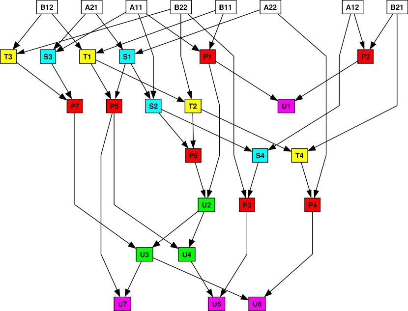
Figure 1: Winograd’s task dependency graph

3 Existing memory placements

Unlike the classic multiplication algorithm, Winograd’s algorithm requires some extra temporary memory allocations to perform its 22 block operations.

3.1 Standard product

We first consider the basic operation $C\leftarrow A\times B$. The best known schedule for this case was given by [6]. We reproduce a similar schedule in table 1.

#​​​​	operation	​​​​loc.	#​​​​	operation	​​​​loc.
1​​​​	$S_{3}=A_{11}-A_{21}$	​​​​$X$	12​​​​	$P_{1}=A_{11}B_{11}$	​​​​$X$
2​​​​	$T_{3}=B_{22}-B_{12}$	​​​​$Y$	13​​​​	$U_{2}=P_{1}+P_{6}$	​​​​$C_{12}$
3​​​​	$P_{7}=S_{3}T_{3}$	​​​​$C_{21}$	14​​​​	$U_{3}=U_{2}+P_{7}$	​​​​$C_{21}$
4​​​​	$S_{1}=A_{21}+A_{22}$	​​​​$X$	15​​​​	$U_{4}=U_{2}+P_{5}$	​​​​$C_{12}$
5​​​​	$T_{1}=B_{12}-B_{11}$	​​​​$Y$	16​​​​	${\bf{U_{7}}}=U_{3}+P_{5}$	​​​​$C_{22}$
6​​​​	$P_{5}=S_{1}T_{1}$	​​​​$C_{22}$	17​​​​	${\bf{U_{5}}}=U_{4}+P_{3}$	​​​​$C_{12}$
7​​​​	$S_{2}=S_{1}-A_{11}$	​​​​$X$	18​​​​	$T_{4}=T_{2}-B_{21}$	​​​​$Y$
8​​​​	$T_{2}=B_{22}-T_{1}$	​​​​$Y$	19​​​​	$P_{4}=A_{22}T_{4}$	​​​​$C_{11}$
9​​​​	$P_{6}=S_{2}T_{2}$	​​​​$C_{12}$	20​​​​	${\bf{U_{6}}}=U_{3}-P_{4}$	​​​​$C_{21}$
10​​​​	$S_{4}=A_{12}-S_{2}$	​​​​$X$	21​​​​	$P_{2}=A_{12}B_{21}$	​​​​$C_{11}$
11​​​​	$P_{3}=S_{4}B_{22}$	​​​​$C_{11}$	22​​​​	${\bf{U_{1}}}=P_{1}+P_{2}$	​​​​$C_{11}$

Table 1: Winograd’s algorithm for operation $C\leftarrow A\times B$, with two temporaries

It requires two temporary blocks $X$ and $Y$ whose dimensions are respectively equal to $m/2\times\max(k/2,n/2)$ and $k/2\times n/2$. Thus the extra memory used is:

$$E_{\ref{tab:schedule:AB}}(m,k,n)=\frac{m}{2}\max{\left(\frac{k}{2},\frac{n}{2}\right)}+\frac{k}{2}\frac{n}{2}+E_{\ref{tab:schedule:AB}}\left(\frac{m}{2},\frac{k}{2},\frac{n}{2}\right).$$

Summing these temporary allocations over every recursive levels leads to a total amount of memory, where for brevity $M=\min{\{m,k,n\}}$:

$$E_{\ref{tab:schedule:AB}}(m,k,n) =\sum_{i=1}^{\log_{2}(M)}\frac{1}{4^{i}}\left(m\max{(k,n)}+kn\right)$$ (1)

$$=\frac{1}{3}\left(1-\frac{1}{M^{2}}\right)\left(m\max{(k,n)}+kn\right)$$

$$<\frac{1}{3}\left(m\max{(k,n)}+kn\right).$$

We can prove in the same manner the following lemma:

Lemma 1.

Let $m$, $k$ and $n$ be powers of two, $g(x,y,z)$ be homogeneous, $M=\min{\{m,k,n\}}$ and $f(m,k,n)$ be a function such that

$$f(m,k,n)=\begin{cases}g\left(\frac{m}{2},\frac{k}{2},\frac{n}{2}\right)+f\left(\frac{m}{2},\frac{k}{2},\frac{n}{2}\right)&\text{if\ }m\text{,\,}n\text{\,and\,}k>1\\ 0&\text{{otherwise.}}\end{cases}$$

Then $f\left(m,k,n\right)=\frac{1}{3}\left(1-\frac{1}{M^{2}}\right)g(m,k,n)<\frac{1}{3}g(m,k,n)$.

In the remainder of the paper, we use $E_{i}$ to denote the amount of extra memory used in table number $i$. The amount of extra memory we consider is always the sum up to the last recursion level.

Finally, assuming $m=n=k$ gives a total extra memory requirement of $E_{\ref{tab:schedule:AB}}(n,n,n)<2/3n^{2}.$

3.2 Product with accumulation

For the more general operation $C\leftarrow\alpha A\times B+\beta C$, a first naïve method would compute the product $\alpha A\times B$ using the scheduling of table 1, into a temporary matrix $C^{\prime}$ and finally compute $C\leftarrow C^{\prime}+\beta C$. It would require $(1+2/3)n^{2}$ extra memory allocations in the square case.
Now the schedule of table 2 due to  [10, fig. 6] only requires 3 temporary blocks for the same number of operations ($7$ multiplications and $4+15$ additions).

#​​​​	operation	​​​​loc.	#​​​​	operation	​​​​loc.
1​​​​	$S_{1}=A_{21}+A_{22}$	​​​​$X$	12​​​​	$S_{4}=A_{12}-S_{2}$	​​​​$X$
2​​​​	$T_{1}=B_{12}-B_{11}$	​​​​$Y$	13​​​​	$T_{4}=T_{2}-B_{21}$	​​​​$Y$
3​​​​	$P_{5}=\alpha S_{1}T_{1}$	​​​​$Z$	14​​​​	$C_{12}=\alpha S_{4}B_{22}+C_{12}$	​​​​$C_{12}$
4​​​​	$C_{22}=P_{5}+\beta C_{22}$	​​​​$C_{22}$	15​​​​	${\bf{U_{5}}}=U_{2}+C_{12}$	​​​​$C_{12}$
5​​​​	$C_{12}=P_{5}+\beta C_{12}$	​​​​$C_{12}$	16​​​​	$P_{4}=\alpha A_{22}T_{4}-\beta C_{21}$	​​​​$C_{21}$
6​​​​	$S_{2}=S_{1}-A_{11}$	​​​​$X$	17​​​​	$S_{3}=A_{11}-A_{21}$	​​​​$X$
7​​​​	$T_{2}=B_{22}-T_{1}$	​​​​$Y$	18​​​​	$T_{3}=B_{22}-B_{12}$	​​​​$Y$
8​​​​	$P_{1}=\alpha A_{11}B_{11}$	​​​​$Z$	19​​​​	$U_{3}=\alpha S_{3}T_{3}+U_{2}$	​​​​$Z$
9​​​​	$C_{11}=P_{1}+\beta C_{11}$	​​​​$C_{11}$	20​​​​	${\bf{U_{7}}}=U_{3}+C_{22}$	​​​​$C_{22}$
10​​​​	$U_{2}=\alpha S_{2}T_{2}+P_{1}$	​​​​$Z$	21​​​​	${\bf{U_{6}}}=U_{3}-C_{21}$	​​​​$C_{21}$
11​​​​	${\bf{U_{1}}}=\alpha A_{12}B_{21}+C_{11}$	​​​​$C_{11}$	22​​​​

Table 2: Schedule for operation $C\leftarrow\alpha A\times B+\beta C$ with 3 temporaries

The required three temporary blocks $X,Y,Z$ have dimensions $m/2\times k/2$, $k/2\times n/2$ and $m/2\times n/2$. Since the two temporary blocks in schedule 1 are smaller than the three ones here, we have $E_{2}\geqslant E_{1}$. Hence, using lemma 1, we get

$$E_{\ref{tab:schedule:ABC}}\left(m,k,n\right)=\frac{1}{3}\left(1-\frac{1}{M^{2}}\right)\left(mk+kn+mn\right).$$ (2)

With $m=n=k$, this gives $E_{\ref{tab:schedule:ABC}}(n,n,n)<n^{2}.$
We propose in table 9 a new schedule for the same operation $\alpha A\times B+\beta C$ only requiring two temporary blocks.
Our new schedule is more efficient if some inner calls overwrite their temporary input matrices. We now present some overwriting schedules and the dynamic program we used to find them.

4 Exhaustive search algorithm

We used a brute force search algorithm to get some of the new schedules that will be presented in the following sections. It is very similar to the pebble game of Huss-Lederman et al. [10].
A sequence of computations is represented as a directed graph, just like figure 1 is built from Winograd’s algorithm.
A node represents a program variable. The nodes can be classified as initials (when they correspond to inputs), temporaries (for intermediate computations) or finals (results or nodes that we want to keep, such as ready-only inputs).
The edges represent the operations; they point from the operands to the result.
A pebble represents an allocated memory. We can put pebbles on any nodes, move or remove them according to a set of simple rules shown below.
When a pebble arrives to a node, the computation at the associated variable starts, and can be “partially” or “fully” executed. If not specified, it is assumed that the computation is fully executed.
Edges can be removed, when the corresponding operation has been computed.
The last two points are especially useful for accumulation operations: for example, it is possible to try schedule the multiplication separately from the addition in an otherwise recursive $AB+C$ call; the edges involved in the multiplication operation would then be removed first and the accumulated part later. They are also useful if we do not want to fix the way some additions are performed: if $U_{3}=P_{1}+P_{6}+P_{7}$ the associativity allows different ways of computing the sum and we let the program explore these possibilities. At the beginning of the exploration, each initial node has a pebble and we may have a few extra available pebbles. The program then tries to apply the following rules, in order, on each node. The program stops when every final node has a pebble or when no further moves of pebbles are possible:

 $\bullet$ Rule 0. Computing a result/removing edges.If a node has a pebble and parents with pebbles, then the operation can be performed and the corresponding edges removed. The node is then at least partially computed.  $\bullet$ Rule 1. Freeing some memory/removing a pebble.If a node is isolated and not final, its pebble is freed. This means that we can reclaim the memory here because this node has been fully computed (no edge pointing to it) and is no longer in use as an operand (no edge initiating from it).  $\bullet$ Rule 2. Computing in place/moving a pebble.If a node $P$ has a full pebble and a single empty child node $S$ and if other parents of $S$ have pebbles on them, then the pebble on $P$ may be transferred to $S$ (corresponding edges are removed). This means an operation has been made in place in the parent $P$’s pebble.  $\bullet$ Rule 3. Using more memory/adding a pebble.If parents of an empty node $N$ have pebbles and a free pebble is available, then this pebble can be assigned to $N$ and the corresponding edges are removed. This means that the operation is computed in a new memory location.  $\bullet$ Rule 4. Copying some memory/duplicating a pebble.A computed node having a pebble can be duplicated. The edges pointed to or from the original node are then rearranged between them. This means that a temporary result has been copied into some free place to allow more flexibility.

5 Overwriting input matrices

We now relax some constraints on the previous problem: the input matrices $A$ and $B$ can be overwritten, as proposed by [13]. For the sake of simplicity, we first give schedules only working for square matrices (i.e. $m=n=k$ and any memory location is supposed to be able to receive any result of any size). We nevertheless give the memory requirements of each schedule as a function of $m$; $k$ and $n$. Therefore it is easier in the last part of this section to adapt the proposed schedules partially for the general case. In the tables, the notation $A_{ij}B_{ij}$ (resp. $A_{ij}B_{ij}+C_{ij})$ denotes the use of the algorithm from table 1 (resp. table 2) as a subroutine. Otherwise we use the notation $Alg(A_{ij}B_{ij})$ to denote a recursive call or the use of one of our new schedules as a subroutine.

5.1 Standard product

We propose in table 3 a new schedule that computes the product $C\leftarrow A\times B$ without any temporary memory allocation. The idea here is to find an ordering where the recursive calls can be made also in place such that the operands of a multiplication are no longer in use after the multiplication has completed because they are overwritten. An exhaustive search showed that no schedule exists overwriting less than four sub-blocks.

#​​​​	operation	​​​​loc.	#​​​​	operation	​​​​loc.
1​​​​	$S_{3}=A_{11}-A_{21}$	​​​​$C_{11}$	12​​​​	$S_{4}=A_{12}-S_{2}$	​​​​$A_{22}$
2​​​​	$S_{1}=A_{21}+A_{22}$	​​​​$A_{21}$	13​​​​	$P_{6}=\texttt{IP}(S_{2}T_{2})$	​​​​$C_{22}$
3​​​​	$T_{1}=B_{12}-B_{11}$	​​​​$C_{22}$	14​​​​	$U_{2}=P_{1}+P_{6}$	​​​​$C_{22}$
4​​​​	$T_{3}=B_{22}-B_{12}$	​​​​$B_{12}$	15​​​​	$P_{2}=\texttt{IP}(A_{12}B_{21})$	​​​​$C_{12}$
5​​​​	$P_{7}=\texttt{IP}(S_{3}T_{3}$)	​​​​$C_{21}$	16​​​​	${\bf{U_{1}}}=P_{1}+P_{2}$	​​​​$C_{11}$
6​​​​	$S_{2}=S_{1}-A_{11}$	​​​​$C_{12}$	17​​​​	$U_{4}=U_{2}+P_{5}$	​​​​$C_{12}$
7​​​​	$P_{1}=\texttt{IP}(A_{11}B_{11})$	​​​​$C_{11}$	18​​​​	$U_{3}=U_{2}+P_{7}$	​​​​$C_{22}$
8​​​​	$T_{2}=B_{22}-T_{1}$	​​​​$B_{11}$	19​​​​	${\bf{U_{6}}}=U_{3}-P_{4}$	​​​​$C_{21}$
9​​​​	$P_{5}=\texttt{IP}(S_{1}T_{1})$	​​​​$A_{11}$	20​​​​	${\bf{U_{7}}}=U_{3}+P_{5}$	​​​​$C_{22}$
10​​​​	$T_{4}=T_{2}-B_{21}$	​​​​$C_{22}$	21​​​​	$P_{3}=\texttt{IP}(S_{4}B_{22})$	​​​​$A_{12}$
11​​​​	$P_{4}=\texttt{IP}(A_{22}T_{4})$	​​​​$A_{21}$	22​​​​	${\bf{U_{5}}}=U_{4}+P_{3}$	​​​​$C_{12}$

Table 3: IP schedule for operation $C\leftarrow A\times B$ in place

Note that this schedule uses only two blocks of $B$ and the whole of $A$ but overwrites all of $A$ and $B$. For instance the recursive computation of $P_{2}$ requires overwriting parts of $A_{12}$ and $B_{21}$ too. Using another schedule as well as back-ups of overwritten parts into some available memory In the following, we will denote by IP for InPlace, either one of these two schedules.
We present in tables 4 and 5 two new schedules overwriting only one of the two input matrices, but requiring an extra temporary space. These two schedules are denoted OvL and OvR. The exhaustive search also showed that no schedule exists overwriting only one of $A$ and $B$ and using no extra temporary.

#​​​​	operation	​​​​loc.	#​​​​	operation	​​​​loc.
1​​​​	$S_{3}=A_{11}-A_{21}$	​​​​$C_{22}$	12​​​​	$P_{6}=\texttt{OvL}(S_{2}T_{2})$	​​​​$C_{21}$
2​​​​	$S_{1}=A_{21}+A_{22}$	​​​​$A_{21}$	13​​​​	$T_{4}=T_{2}-B_{21}$	​​​​$A_{11}$
3​​​​	$S_{2}=S_{1}-A_{11}$	​​​​$C_{12}$	14​​​​	$U_{2}=P_{1}+P_{6}$	​​​​$C_{21}$
4​​​​	$T_{1}=B_{12}-B_{11}$	​​​​$C_{21}$	15​​​​	$U_{4}=U_{2}+P_{5}$	​​​​$C_{12}$
5​​​​	$P_{1}=\texttt{OvL}(A_{11}B_{11})$	​​​​$C_{11}$	16​​​​	$U_{3}=U_{2}+P_{7}$	​​​​$C_{21}$
6​​​​	$T_{3}=B_{22}-B_{12}$	​​​​$A_{11}$	17​​​​	${\bf{U_{7}}}=U_{3}+P_{5}$	​​​​$C_{22}$
7​​​​	$P_{7}=\texttt{IP}(S_{3}T_{3})$	​​​​$X$	18​​​​	${\bf{U_{5}}}=U_{4}+P_{3}$	​​​​$C_{12}$
8​​​​	$T_{2}=B_{22}-T_{1}$	​​​​$A_{11}$	19​​​​	$P_{2}=\texttt{OvL}(A_{12}B_{21})$	​​​​$X$
9​​​​	$P_{5}=\texttt{IP}(S_{1}T_{1})$	​​​​$C_{22}$	20​​​​	${\bf{U_{1}}}=P_{1}+P_{2}$	​​​​$C_{11}$
10​​​​	$S_{4}=A_{12}-S_{2}$	​​​​$C_{21}$	21​​​​	$P_{4}=\texttt{IP}(A_{22}T_{4})$	​​​​$A_{21}$
11​​​​	$P_{3}=\texttt{OvL}(S_{4}B_{22})$	​​​​$A_{21}$	22​​​​	${\bf{U_{6}}}=U_{3}-P_{4}$	​​​​$C_{21}$

Table 4: OvL schedule for operation $C\leftarrow A\times B$ using strictly two blocks of $A$ and one temporary

#​​​​	operation	​​​​loc.	#​​​​	operation	​​​​loc.
1​​​​	$S_{3}=A_{11}-A_{21}$	​​​​$C_{22}$	12​​​​	$P_{4}=\texttt{OvR}(A_{22}T_{4})$	​​​​$B_{12}$
2​​​​	$S_{1}=A_{21}+A_{22}$	​​​​$C_{21}$	13​​​​	$S_{4}=A_{12}-S_{2}$	​​​​$B_{11}$
3​​​​	$T_{1}=B_{12}-B_{11}$	​​​​$C_{12}$	14​​​​	$U_{2}=P_{1}+P_{6}$	​​​​$C_{21}$
4​​​​	$P_{1}=\texttt{OvR}(A_{11}B_{11})$	​​​​$C_{11}$	15​​​​	$U_{4}=U_{2}+P_{5}$	​​​​$C_{12}$
5​​​​	$S_{2}=S_{1}-A_{11}$	​​​​$B_{11}$	16​​​​	$U_{3}=U_{2}+P_{7}$	​​​​$C_{21}$
6​​​​	$T_{3}=B_{22}-B_{12}$	​​​​$B_{12}$	17​​​​	${\bf{U_{7}}}=U_{3}+P_{5}$	​​​​$C_{22}$
7​​​​	$P_{7}=\texttt{IP}(S_{3}T_{3})$	​​​​$X$	18​​​​	${\bf{U_{6}}}=U_{3}-P_{4}$	​​​​$C_{21}$
8​​​​	$T_{2}=B_{22}-T_{1}$	​​​​$B_{12}$	19​​​​	$P_{3}=\texttt{IP}(S_{4}B_{22})$	​​​​$B_{12}$
9​​​​	$P_{5}=\texttt{IP}(S_{1}T_{1})$	​​​​$C_{22}$	20​​​​	${\bf{U_{5}}}=U_{4}+P_{3}$	​​​​$C_{12}$
10​​​​	$T_{4}=T_{2}-B_{21}$	​​​​$C_{12}$	21​​​​	$P_{2}=\texttt{OvR}(A_{12}B_{21})$	​​​​$B_{12}$
11​​​​	$P_{6}=\texttt{OvR}(S_{2}T_{2})$	​​​​$C_{21}$	22​​​​	${\bf{U_{1}}}=P_{1}+P_{2}$	​​​​$C_{11}$

Table 5: OvR schedule for operation $C\leftarrow A\times B$ using strictly two blocks of $B$ and one temporary

We note that we can overwrite only two blocks of $A$ in OvL when the schedule is modified as follows:

#​​​​	operation	​​​​loc.
18bis​​​​	$A_{21}=\texttt{Copy}(A_{12})$	​​​​$A_{21}$
19bis​​​​	$A_{12}=\texttt{Copy}(A_{21})$	​​​​$A_{12}$
21​​​​	$P_{4}=\texttt{OvR}(A_{22}T_{4})$	​​​​$A_{21}$

Similarly, for OvR, we can overwrite only two blocks of $B$ using copies on lines 20 and 21 and OvL on line 19.
We now compute the extra memory needed for the schedule of table 5. The size of the temporary block $X$ is $\left(\frac{n}{2}\right)^{2}$, the extra memory required for table 5 hence satisfies: $E_{\ref{tab:AB:ipright}}(n,n,n)<\frac{1}{3}n^{2}$.

5.2 Product with accumulation

We now consider the operation $C\leftarrow\alpha A\times B+\beta C$, where the input matrices $A$ and $B$ can be overwritten. We propose in table 6 a schedule that only requires $2$ temporary block matrices, instead of the $3$ in table 2. This is achieved by overwriting the inputs and by using two additional pre-additions ($Z_{1}$ and $Z_{2}$) on the matrix $C$.

#​​​​​​	operation	​​​​​​loc.	#​​​​​​	operation	​​​​​​loc.
1​​​​​​	$Z_{1}=C_{22}-C_{12}$	​​​​​​$C_{22}$	13​​​​​​	$P_{4}=\texttt{AcLR}(\alpha A_{22}T_{4}{-\beta Z_{2}})$	​​​​​​$C_{21}$
2​​​​​​	$S_{1}=A_{21}+A_{22}$	​​​​​​$X$	14​​​​​​	$S_{4}=A_{12}-S_{2}$	​​​​​​$A_{22}$
3​​​​​​	$T_{1}=B_{12}-B_{11}$	​​​​​​$Y$	15​​​​​​	$P_{6}=\alpha\texttt{IP}(S_{2}T_{2})$	​​​​​​$X$
4​​​​​​	$Z_{2}=C_{21}-Z_{1}$	​​​​​​$C_{21}$	16​​​​​​	$P_{2}=\texttt{AcLR}(\alpha A_{12}B_{21}{+\beta C_{11}})$	​​​​​​$C_{11}$
5​​​​​​	$T_{3}=B_{22}-B_{12}$	​​​​​​$B_{12}$	17​​​​​​	${\bf{U_{1}}}=P_{1}+P_{2}$	​​​​​​$C_{11}$
6​​​​​​	$S_{3}=A_{11}-A_{21}$	​​​​​​$A_{21}$	18​​​​​​	$U_{2}=P_{1}+P_{6}$	​​​​​​$X$
5​​​​​​	$P_{7}=\texttt{AcLR}(\alpha S_{3}T_{3}{+\beta Z_{1}})$	​​​​​​$C_{22}$	17​​​​​​	$U_{3}=U_{2}+P_{7}$	​​​​​​$C_{22}$
8​​​​​​	$S_{2}=S_{1}-A_{11}$	​​​​​​$A_{21}$	20​​​​​​	$U_{4}=U_{2}+P_{5}$	​​​​​​$X$
9​​​​​​	$T_{2}=B_{22}-T_{1}$	​​​​​​$B_{12}$	21​​​​​​	${\bf{U_{6}}}=U_{3}-P_{4}$	​​​​​​$C_{21}$
10​​​​​​	$P_{5}=\texttt{AcLR}(\alpha S_{1}T_{1}{+\beta C_{12}})$	​​​​​​$C_{12}$	22​​​​​​	${\bf{U_{7}}}=U_{3}+P_{5}$	​​​​​​$C_{22}$
11​​​​​​	$P_{1}=\alpha\texttt{IP}(A_{11}B_{11})$	​​​​​​$Y$	23​​​​​​	$P_{3}=\alpha\texttt{IP}(S_{4}B_{22})$	​​​​​​$C_{12}$
12​​​​​​	$T_{4}=T_{2}-B_{21}$	​​​​​​$X$	24​​​​​​	${\bf{U_{5}}}=U_{4}+P_{3}$	​​​​​​$C_{12}$

Table 6: AcLR schedule for $C\leftarrow\alpha A\times B+\beta C$ overwriting $A$ and $B$ with 2 temporaries, 4 recursive calls

We also propose in table 7 a schedule similar to table 6 overwriting only for instance the right input matrix. It also uses only two temporaries, but has to call the OvR schedule. The extra memory required by $X$ and $Y$ in table 6 is $2\left(\frac{n}{2}\right)^{2}$. Hence, using lemma 1:

$$E_{\ref{tab:ABC:overwrite}}(n,n,n)<\frac{2}{3}n^{2}.$$ (3)

#​​​​​​	operation	​​​​​​loc.	#​​​​​​	operation	​​​​​​loc.
1​​​​​​	$Z_{1}=C_{22}-C_{12}$	​​​​​​$C_{22}$	13​​​​​​	$P_{2}=\texttt{AccR}(\alpha A_{12}B_{21}{+\beta C_{11}})$	​​​​​​$C_{11}$
2​​​​​​	$T_{1}=B_{12}-B_{11}$	​​​​​​$X$	14​​​​​​	$S_{2}=S_{1}-A_{11}$	​​​​​​$Y$
3​​​​​​	$Z_{2}=C_{21}-Z_{1}$	​​​​​​$C_{21}$	15​​​​​​	$P_{6}=\alpha\texttt{OvR}(S_{2}T_{2})$	​​​​​​$B_{21}$
4​​​​​​	$T_{3}=B_{22}-B_{12}$	​​​​​​$B_{12}$	16​​​​​​	$S_{4}=A_{12}-S_{2}$	​​​​​​$Y$
5​​​​​​	$S_{3}=A_{11}-A_{21}$	​​​​​​$Y$	17​​​​​​	$U_{2}=P_{1}+P_{6}$	​​​​​​$B_{21}$
6​​​​​​	$P_{7}=\texttt{AccR}(\alpha S_{3}T_{3}{+\beta Z_{1}})$	​​​​​​$C_{22}$	18​​​​​​	$U_{3}=U_{2}+P_{7}$	​​​​​​$C_{22}$
7​​​​​​	$S_{1}=A_{21}+A_{22}$	​​​​​​$Y$	19​​​​​​	$U_{4}=U_{2}+P_{5}$	​​​​​​$B_{21}$
8​​​​​​	$T_{2}=B_{22}-T_{1}$	​​​​​​$B_{12}$	20​​​​​​	${\bf{U_{6}}}=U_{3}-P_{4}$	​​​​​​$C_{21}$
9​​​​​​	$P_{5}=\texttt{AccR}(\alpha S_{1}T_{1}{+\beta C_{12}})$	​​​​​​$C_{12}$	21​​​​​​	${\bf{U_{1}}}=P_{1}+P_{2}$	​​​​​​$C_{11}$
10​​​​​​	$T_{4}=T_{2}-B_{21}$	​​​​​​$X$	22​​​​​​	${\bf{U_{7}}}=U_{3}+P_{5}$	​​​​​​$C_{22}$
11​​​​​​	$P_{4}=\texttt{AccR}(\alpha A_{22}T_{4}{-\beta Z_{2}})$	​​​​​​$C_{21}$	23​​​​​​	$P_{3}=\alpha\texttt{IP}(S_{4}B_{22})$	​​​​​​$C_{12}$
12​​​​​​	$P_{1}=\alpha\texttt{OvR}(A_{11}B_{11})$	​​​​​​$X$	24​​​​​​	${\bf{U_{5}}}=U_{4}+P_{3}$	​​​​​​$C_{12}$

Table 7: AccR schedule for $C\leftarrow\alpha A\times B+\beta C$ overwriting $B$ with 2 temporaries, 4 recursive calls

The extra memory $E_{\ref{tab:ABC:overright}}(n,n,n)$ required for table 7 in the top level of recursion is:

$$\left(\frac{n}{2}\right)^{2}+\left(\frac{n}{2}\right)^{2}+\max{\left(E_{\ref{tab:ABC:overright}},E_{\ref{tab:AB:ipright}}\right)}\left(\frac{n}{2},\frac{n}{2},\frac{n}{2}\right).$$

We clearly have $E_{\ref{tab:ABC:overright}}>E_{\ref{tab:AB:ipright}}$ and:

$$E_{\ref{tab:ABC:overright}}(n,n,n)<\frac{2}{3}n^{2}.$$

Compared with the schedule of table 2, the possibility to overwrite the input matrices makes it possible to have further in place calls and replace recursive calls with accumulation by calls without accumulation. We show in theorem 3 that this enables us to almost compensate for the extra additions performed.

5.3 The rectangular case

We now examine the sizes of the temporary locations used, when the matrices involved do not have identical sizes. We want to make use of table 3 for the general case.
Firstly, the sizes of $A$ and $B$ must not be bigger than that of $C$ (i.e. we need $k\leqslant\min{(m,n)}$). Indeed, let’s play a pebble game that we start with pebbles on the inputs and $4$ extra pebbles that are the size of a $C_{ij}$. No initial pebble can be moved since at least two edges initiate from the initial nodes. If the size of $A_{ij}$ is larger that the size of the free pebbles, then we cannot put a free pebble on the $S_{i}$ nodes (they are too large). We cannot put either a pebble on $P_{1}$ or $P_{2}$ since their operands would be overwritten. So the size of $A_{ij}$ is smaller or equal than that of $C_{ij}$. The same reasoning applies for $B_{ij}$.
Then, if we consider a pebble game that was successful, we can prove in the same fashion that either the size of $A$ or the size of $B$ can not be smaller that of $C$ (so one of them has the same size as $C$).
Finally, table 3 shows that this is indeed possible, with $k=n\leqslant m$. It is also possible to switch the roles of $m$ and $n$.
Now in tables 4 to 7, we need that $A$, $B$ and $C$ have the same size. Generalizing table 3 whenever we do not have a dedicated in-place schedule can then done by cutting the larger matrices in squares of dimension $\min{(m,k,n)}$ and doing the multiplications / product with accumulations on these smaller matrices using algorithm 1 to 7 and free space from $A$, $B$ or $C$.Since algorithms 1 to 7 require less than $n^{2}$ extra memory, we can use them as soon as one small matrix is free.
We now propose an example in algorithm 1 for the case $n<\min{(m,k)}$:

1:$A$ and $B$ of resp. sizes $m\times k$ and $k\times n$

2:$n<\min{(m,k)}$ and $m$, $k$, $n$ powers of $2$.

3:$C=A\times B$

4:Let $k_{0}=k/n$ and $m_{0}=m/n$.

5:Split $A=\left[\small\begin{array}[]{c|c|c}A_{1,1}&\dots&A_{1,k_{0}}\\ \hline\cr\vdots&&\vdots\\ \hline\cr A_{m_{0},1}&\dots&A_{m_{0},k_{0}}\\ \end{array}\right]$, $B=\left[\small\begin{array}[]{c}B_{1}\\ \hline\cr\vdots\\ \hline\cr B_{k_{0}}\end{array}\right]$ and $C=\left[\small\begin{array}[]{c}C_{1}\\ \hline\cr\vdots\\ \hline\cr C_{k_{0}}\end{array}\right]$ $\triangleright$ where $A_{i,j}$ and $B_{j}$ have dimension $n\times n$

6:$C_{1}\leftarrow A_{1,1}B_{1}$ $\triangleright$ with alg. of table 1 and memory $C_{2}$.

7:Now we use $A_{1,1}$ as temporary space.

8:for $i=2\dots k_{0}$ do

9:     $C_{i}\leftarrow A_{i,1}B_{1}$ $\triangleright$ with alg. of table 4.

10:end for

11:for $j=2\dots k_{0}$ do

12:     for $i=1\dots m_{0}$ do

13:         $C_{j}\leftarrow A_{i,j}B_{j}+C_{j}$ $\triangleright$ with alg. of table 2.

14:     end for

15:end for

Algorithm 1 IP0vMM: In-Place Overwrite Matrix Multiply

Proposition 1.

Algorithm 1 computes the product $C=AB$ in place, overwriting $A$ and $B$.

Finally, we generalize the accumulation operation from table 7 to the rectangular case. We can no longer use dedicated square algorithms. This is done in table 8, overwriting only one of the inputs and using only two temporaries, but with 5 recursive accumulation calls:

#​​​​​​	operation	​​​​​​loc.	#​​​​​​	operation	​​​​​​loc.
1​​​​​​	$Z_{1}=C_{22}-C_{12}$	​​​​​​$C_{22}$	13​​​​​​	$P_{2}=\texttt{AcR}(\alpha A_{12}B_{21}{+\beta C_{11}})$	​​​​​​$C_{11}$
2​​​​​​	$T_{1}=B_{12}-B_{11}$	​​​​​​$X$	14​​​​​​	${\bf{U_{1}}}=P_{1}+P_{2}$	​​​​​​$C_{11}$
3​​​​​​	$Z_{2}=C_{21}-Z_{1}$	​​​​​​$C_{21}$	15​​​​​​	$S_{2}=S_{1}-A_{11}$	​​​​​​$Y$
4​​​​​​	$T_{3}=B_{22}-B_{12}$	​​​​​​$B_{12}$	16​​​​​​	$U_{2}=\texttt{AcR}(\alpha S_{2}T_{2}{+P_{1}})$	​​​​​​$X$
5​​​​​​	$S_{3}=A_{11}-A_{21}$	​​​​​​$Y$	17​​​​​​	$U_{3}=U_{2}+P_{7}$	​​​​​​$C_{22}$
6​​​​​​	$P_{7}=\texttt{AcR}(\alpha S_{3}T_{3}{+\beta Z_{1}})$	​​​​​​$C_{22}$	18​​​​​​	${\bf{U_{6}}}=U_{3}-P_{4}$	​​​​​​$C_{21}$
7​​​​​​	$S_{1}=A_{21}+A_{22}$	​​​​​​$Y$	19​​​​​​	${\bf{U_{7}}}=U_{3}+P_{5}$	​​​​​​$C_{22}$
8​​​​​​	$T_{2}=B_{22}-T_{1}$	​​​​​​$B_{12}$	20​​​​​​	$U_{4}=U_{2}+P_{5}$	​​​​​​$X$
9​​​​​​	$P_{5}=\texttt{AcR}(\alpha S_{1}T_{1}{+\beta C_{12}})$	​​​​​​$C_{12}$	21​​​​​​	$S_{4}=A_{12}-S_{2}$	​​​​​​$Y$
10​​​​​​	$T_{4}=T_{2}-B_{21}$	​​​​​​$X$	22​​​​​​	$P_{3}=\alpha S_{4}B_{22}$	​​​​​​$C_{12}$
11​​​​​​	$P_{4}=\texttt{AcR}(\alpha A_{22}T_{4}{-\beta Z_{2}})$	​​​​​​$C_{21}$	23​​​​​​	${\bf{U_{5}}}=U_{4}+P_{3}$	​​​​​​$C_{12}$
12​​​​​​	$P_{1}=\alpha A_{11}B_{11}$	​​​​​​$X$	24​​​​​​

Table 8: AcR schedule for $C\leftarrow\alpha A\times B+\beta C$ with 5 recursive calls, 2 temporaries and overwriting $B$

For instance, in table 8, the last multiplication (line 22, $P_{3}=\alpha S_{4}B_{22}$) could have been made by a call to the in place algorithm, would $C_{12}$ be large enough. This is not always the case in a rectangular setting.

Now, the size of the extra temporaries required in table 8 is $\max{\left(\frac{m}{2},\frac{k}{2}\right)}\frac{n}{2}+\frac{m}{2}\frac{k}{2}$ and $E_{\ref{tab:ABC:overright:gen}}(m,k,n)$ is equal to:

$$\max{\left(\frac{m}{2},\frac{k}{2}\right)}\frac{n}{2}+\frac{m}{2}\frac{k}{2}+\max{\left(E_{\ref{tab:ABC:overright:gen}},E_{\ref{tab:schedule:AB}}\right)}\left(\frac{m}{2},\frac{k}{2},\frac{n}{2}\right).$$

If $m<k<n$ or $k<m<n$, then $E_{\ref{tab:ABC:overright:gen}}(m,k,n)<E_{\ref{tab:schedule:AB}}(m,k,n)$:

$$E_{\ref{tab:ABC:overright:gen}}(m,k,n) =\max{\left(\frac{m}{2},\frac{k}{2}\right)}\frac{n}{2}+\frac{m}{2}\frac{k}{2}+E_{\ref{tab:schedule:AB}}\left(\frac{m}{2},\frac{k}{2},\frac{n}{2}\right)$$

$$<\max{\left(\frac{m}{2},\frac{k}{2}\right)}\frac{n}{2}+\frac{m}{2}\frac{k}{2}+\frac{1}{3}\left(\frac{m}{2}\frac{n}{2}+\frac{k}{2}\frac{n}{2}\right).$$

Otherwise $E_{\ref{tab:ABC:overright:gen}}(m,k,n)\geqslant E_{\ref{tab:schedule:AB}}(m,k,n)$ and:

$$E_{\ref{tab:ABC:overright:gen}}(m,k,n)<\frac{1}{3}\left(\max{\left(m,k\right)}n+mk\right).$$

In the square case, this simplifies into $E_{\ref{tab:ABC:overright:gen}}(n,n,n)\leqslant\frac{2}{3}n^{2}.$

In addition, if the size of $B$ is bigger than that of $A$, then one can store $S_{2}$, for instance within $B_{12}$, and separate the recursive call $16$ into a multiplication and an addition, which reduces the arithmetic complexity. Otherwise, a scheduling with only 4 recursive calls exists too, but we need for instance to recompute $S_{4}$ at step $21$.

6 Hybrid scheduling

By combining techniques from sections 3 and 5, we now propose in table 9 a hybrid algorithm that performs the computation $C\leftarrow\alpha A\times B+\beta C$ with constant input matrices $A$ and $B$, with a lower extra memory requirement than the scheduling of  [10] (table 2). We have to pay a price of order $n^{2}\log(n)$ extra operations, as we need to compute the temporary variable $T_{2}$ twice.

#​​​​​​	operation	​​​​​​loc.	#​​​​​​	operation	​​​​​​loc.
1​​​​​​	$Z_{1}=C_{22}-C_{12}$	​​​​​​$C_{22}$	14​​​​​​	$P_{2}=\texttt{Acc}(\alpha A_{12}B_{21}{+\beta C_{11}})$	​​​​​​$C_{11}$
2​​​​​​	$Z_{3}=C_{12}-C_{21}$	​​​​​​$C_{12}$	15​​​​​​	${\bf{U_{1}}}=P_{1}+P_{2}$	​​​​​​$C_{11}$
3​​​​​​	$S_{1}=A_{21}+A_{22}$	​​​​​​$X$	16​​​​​​	${\bf{U_{5}}}=U_{2}+P_{3}$	​​​​​​$C_{12}$
4​​​​​​	$T_{1}=B_{12}-B_{11}$	​​​​​​$Y$	17​​​​​​	$S_{3}=A_{11}-A_{21}$	​​​​​​$X$
5​​​​​​	$P_{5}=\texttt{Acc}(\alpha S_{1}T_{1}{+\beta Z_{3}})$	​​​​​​$C_{12}$	18​​​​​​	$T_{3}=B_{22}-B_{12}$	​​​​​​$Y$
6​​​​​​	$S_{2}=S_{1}-A_{11}$	​​​​​​$X$	19​​​​​​	$U_{3}=P_{7}+U_{2}$	​​​​​​$C_{21}$
7​​​​​​	$T_{2}=B_{22}-T_{1}$	​​​​​​$Y$		$\phantom{U_{3}}=\alpha\texttt{AcLR}(S_{3}T_{3}{+U_{2}})$
8​​​​​​	$P_{6}=\texttt{Acc}(\alpha S_{2}T_{2}{+\beta C_{21}})$	​​​​​​$C_{21}$	20​​​​​​	${\bf{U_{7}}}=U_{3}+W_{1}$	​​​​​​$C_{22}$
9​​​​​​	$S_{4}=A_{12}-S_{2}$	​​​​​​$X$	21​​​​​​	$T_{1}^{\prime}=B_{12}-B_{11}$	​​​​​​$Y$
10​​​​​​	$W_{1}=P_{5}+\beta Z_{1}$	​​​​​​$C_{22}$	22​​​​​​	$T_{2}^{\prime}=B_{22}-T_{1}^{\prime}$	​​​​​​$Y$
11​​​​​​	$P_{3}=\texttt{Acc}(\alpha S_{4}B_{22}{+P_{5}})$	​​​​​​$C_{12}$	23​​​​​​	$T_{4}=T_{2}^{\prime}-B_{21}$	​​​​​​$Y$
12​​​​​​	$P_{1}=\alpha A_{11}B_{11}$	​​​​​​$X$	24​​​​​​	${\bf{U_{6}}}=U_{3}-P_{4}$	​​​​​​$C_{21}$
13​​​​​​	$U_{2}=P_{6}+P_{1}$	​​​​​​$C_{21}$		$\phantom{{\bf{U_{6}}}}=-\alpha\texttt{AccR}(A_{22}T_{4}{-U_{3}})$

Table 9: Acc schedule for operation $C\leftarrow\alpha A\times B+\beta C$ with 2 temporaries

Again, the two temporary blocks $X$ and $Y$ have dimensions $X_{s}=Y_{s}=(n/2)^{2}$ so that:

$$E_{\ref{tab:ABC:2tmp}}=Y_{s}+\max{\left\{X_{s}+E_{\ref{tab:ABC:2tmp}},X_{s}+E_{\ref{tab:ABC:overwrite}},E_{\ref{tab:ABC:overright:gen}}\right\}}\left(\frac{m}{2},\frac{k}{2},\frac{n}{2}\right).$$

In all cases, $E_{\ref{tab:ABC:overwrite}}+X_{s}\geqslant E_{\ref{tab:ABC:overright:gen}}.$ But $X_{s}+Y_{s}$ is not as large as the size of the two temporaries in table 6. We therefore get:

$$E_{\ref{tab:ABC:2tmp}}(m,k,n)={} Y_{s}+X_{s}+E_{\ref{tab:ABC:overwrite}}\left(\frac{m}{2},\frac{k}{2},\frac{n}{2}\right)$$

$$<{} 2\left(\frac{n}{2}\right)^{2}+\frac{1}{3}\left(\left(\frac{n}{2}\right)^{2}+\left(\frac{n}{2}\right)^{2}\right).$$

Assuming $m=n=k$, one gets $E_{\ref{tab:ABC:2tmp}}(n,n,n)<\frac{2}{3}n^{2},$ which is smaller than the extra memory requirement of table 2.

7 A sub-cubic in-place algorithm

Following the improvements of the previous section, the question was raised whether extra memory allocation was intrinsic to sub-cubic matrix multiplication algorithms. More precisely, is there a matrix multiplication algorithm computing $C\leftarrow A\times B$ in $\mathcal{O}\left(n^{\log_{2}7}\right)$ arithmetic operations without extra memory allocation and without overwriting its input arguments? We show in this section that a combination of Winograd’s algorithm and a classic block algorithm provides a positive answer. Furthermore this algorithm also improves the extra memory requirement for the product with accumulation $C\leftarrow\alpha A\times B+\beta C$.

7.1 The algorithm

The key idea is to split the result matrix $C$ into four quadrants of dimension $n/2\times n/2$. The first three quadrants $C_{11},C_{12}$ and $C_{21}$ are computed using fast rectangular matrix multiplication, which accounts for $2k/n$ standard Winograd multiplications on blocks of dimension $n/2\times n/2$. The temporary memory for these computations is stored in $C_{22}$. Lastly, the block $C_{22}$ is computed recursively up to a base case, as shown on algorithm 2. This base case, when the matrix is too small to benefit from the fast routine, is then computed with the classical matrix multiplication.

1:$A$ and $B$, of dimensions resp. $n\times k$ and $k\times n$ with $k$, $n$ powers of 2 and $k\geqslant n$.

2:$C=A\times B$

3:Split $C=\begin{bmatrix}C_{11}&C_{12}\\ C_{21}&C_{22}\end{bmatrix}$, $A=\left[\small\begin{array}[]{c|c|c}A_{1,1}&\dots&A_{1,2k/n}\\ \hline\cr A_{2,1}&\dots&A_{2,2k/n}\end{array}\right]$ and $B=\left[\small\begin{array}[]{c|c}B_{1,1}&B_{1,2}\\ \hline\cr\vdots&\vdots\\ \hline\cr B_{2k/n,1}&B_{2k/n,2}\end{array}\right]$ $\triangleright$ where each $A_{i,j},B_{i,j}$ and $C_{i,j}$ have dimension $n/2\times n/2$.

4:do$\triangleright$ with alg. of table 1 using $C_{22}$ as temp. space

5:     $C_{11}=A_{1,1}B_{1,1}$

6:     $C_{12}=A_{1,1}B_{1,2}$

7:     $C_{21}=A_{2,1}B_{1,1}$

8:end do

9:for $i=2\dots\frac{2k}{n}$ do $\triangleright$ with alg. of table 2 using $C_{22}$ as temporary space:

10:     $C_{11}=A_{1,i}B_{i,1}+C_{11}$

11:     $C_{12}=A_{1,i}B_{i,2}+C_{12}$

12:     $C_{21}=A_{2,i}B_{i,1}+C_{21}$

13:end for

14:$C_{22}=A_{2,*}\times B_{*,2}$ $\triangleright$ recursively using IPMM.

Algorithm 2 IPMM: In-Place Matrix Multiply

Theorem 1.

The complexity of algorithm 2 is:

$$G(n,n)=7.2n^{\log_{2}(7)}-13n^{2}+6.8n$$

when $k=n$.

Proof.

Recall that the cost of Winograd’s algorithm for square matrices is $W(n)=6n^{\log_{2}7}-5n^{2}$ for the operation $C\leftarrow A\times B$ and $W_{\text{acc}}(n)=6n^{\log_{2}7}-4n^{2}$ for the operation $C\leftarrow A\times B+C$. The cost $G(n,k)$ of algorithm 2 is given by the relation

$$G(n,k)=3W(n/2)+3(2k/n-1)W_{\text{acc}}(n/2)+G(n/2,k),$$

the base case being a classical dot product: $G(1,k)=2k-1$. Thus, $G(n,k)=7.2kn^{\log_{2}(7)-1}-12kn-n^{2}+34k/5$. ∎

Theorem 2.

For any $m$, $n$ and $k$, algorithm 2 is in place.

Proof.

W.l.o.g, we assume that $m\geqslant n>1$ (otherwise we could use the transpose). The exact amount of extra memory from algorithms in table 1 and 2 is respectively given by eq. (1) and (2).
If we cut $B$ into $p_{i}$ stripes at recursion level $i$, then the sizes for the involved submatrices of $A$ (resp. $B$) are $m/2^{i}\times k/p_{i}$ (reps. $k/p_{i}\times n/2^{i}$). The lower right corner submatrix of $C$ that we would like to use as temporary space has a size $m/2^{i}\times n/2^{i}$. Thus we need to ensure that the following inequality holds:

$$\max{(E_{\ref{tab:schedule:AB}},E_{\ref{tab:schedule:ABC}})}\left(\frac{m}{2^{i}},\frac{k}{p_{i}},\frac{n}{2^{i}}\right)\leqslant\frac{m}{2^{i}}\frac{n}{2^{i}}.$$ (4)

It is clear that $E_{\ref{tab:schedule:AB}}<E_{\ref{tab:schedule:ABC}},$ which simplifies the previous inequality. Let us now write $K=k/p_{i}$, $M=m/2^{i}$ and $N=n/2^{i}$. We need to find, for every $i$ an integer $p_{i}>1$ so that eq. (4) holds. In other words, let us show that there exists some $K<k$ such that, for any $(M,N)$, the inequality $E_{\ref{tab:schedule:ABC}}(M,K,N)\leqslant MN$ holds. Then the fact that $E(M,2,N)<\frac{1}{3}(2M+2N+MN)\leqslant\frac{1}{3}(4M+MN)\leqslant MN$ provides at least one such $K$.
As the requirements in algorithm 2 ensure that $k>N$ and $M=N$, there just remains to prove that $E(M,N,N)\leqslant MN$. Since $E(M,N,N)<\frac{1}{3}(2MN+N^{2})$ and again $M\geqslant N$, algorithm 2 is indeed in place. ∎

Hence a fully in-place $\mathcal{O}\left(n^{\log_{2}7}\right)$ algorithm is obtained for matrix multiplication. The overhead of this approach appears in the multiplicative constant of the leading term of the complexity, growing from $6$ to $7.2$.
This approach extends to the case of matrices with general dimensions, using for instance peeling or padding techniques.
It is also useful if any sub-cubic algorithm is used instead of Winograd’s. For instance, in the square case, one can use the product with accumulation in table 9 instead of table 2.

7.2 Reduced memory usage for the product with accumulation

In the case of computing the product with accumulation, the matrix $C$ can no longer be used as temporary storage, and extra memory allocation cannot be avoided. Again we can use the idea of the classical block matrix multiplication at the higher level and call Winograd algorithm for the block multiplications. As in the previous subsection, $C$ can be divided into four blocks and then the product can be made with 8 calls to Winograd algorithm for the smaller blocks, with only one extra temporary block of dimension $n/2\times n/2$.
More generally, for square $n\times n$ matrices, $C$ can be divided in $t^{2}$ blocks of dimension $\frac{n}{t}\times\frac{n}{t}$. Then one can compute each block with Winograd algorithm using only one extra memory chunk of size $(n/t)^{2}$. The complexity is changed to $R_{t}(n)=t^{2}tW_{\text{acc}}(n/t),$ which is $R_{t}(n)=6t^{3-\log_{2}(7)}n^{\log_{2}(7)}-4tn^{2}$ for an accumulation product with Winograd’s algorithm. Using the parameter $t$, one can then balance the memory usage and the extra arithmetic operations. For example, with $t=2$,

$$R_{2}=6.857n^{\log_{2}7}-8n^{2}~{}~{}\text{and}~{}~{}\text{ExtraMem}=\frac{n^{2}}{4}$$

and with $t=3$,

$$R_{3}=7.414n^{\log_{2}7}-12n^{2}~{}~{}\text{and}~{}~{}\text{ExtraMem}=\frac{n^{2}}{9}.$$

Note that one can use the algorithm of table 9 instead of the classical Winograd accumulation as the base case algorithm. Then the memory overhead drops down to $\frac{2n^{2}}{3t^{2}}$ and the arithmetic complexity increases to $R_{t}(n)+t^{2-\log_{2}(3)}n^{\log_{2}(6)}-tn^{2}$.

8 Conclusion

With constant input matrices, we reduced the number of extra memory allocations for the operation $C\leftarrow\alpha A\times B+\beta C$ from $n^{2}$ to $\frac{2}{3}n^{2}$, by introducing two extra pre-additions. As shown below, the overhead induced by these supplementary additions is amortized by the gains in number of memory allocations.

If the input matrices can be overwritten, we proposed a fully in-place schedule for the operation $C\leftarrow A\times B$ without any extra operations. We also proposed variants for the operation $C\leftarrow A\times B$, where only one of the input matrices is being overwritten and one temporary is required. These subroutines allow us to reduce the extra memory allocations required for the $C\leftarrow\alpha A\times B+\beta C$ operation without overwrite: the extra required temporary space drops from $n^{2}$ to only $\frac{2}{3}n^{2}$, at a negligible cost.

Some algorithms with an even more reduced memory usage, but with some increase in arithmetic complexity, are also shown. Table 10 gives a summary of the features of each schedule that has been presented. The complexities are given only for $m=k=n$ being a power of $2$.

	Algorithm	Input matrices	# of extra temporaries	total extra memory	total # of extra allocations	arithmetic complexity
$A\times B$	Table 1 [6]	Constant	$2$	$\frac{2}{3}n^{2}$	$\frac{2}{3}(n^{2.807}-n^{2})$	$6n^{2.807}-5n^{2}$
	Table 3	Both Overwritten	$0$	$0$	$0$	$6n^{2.807}-5n^{2}$
	Table 4 or 5	$A$ or $B$ Overwritten	$1$	$\frac{1}{3}n^{2}$	$\frac{1}{4}n^{2}\log_{2}(n)$	$6n^{2.807}-5n^{2}$
	7.1	Constant	$0$	$0$	$0$	$7.2n^{2.807}-13n^{2}$
$\alpha A\times B+\beta C$	Table 2 [10]	Constant	$3$	$n^{2}$	$\frac{2}{3}n^{\log_{2}(7)}+n^{\log_{2}(5)}-\frac{5}{3}n^{2}$	$6n^{2.807}-4n^{2}$
	Table 6	Both Overwritten	$2$	$\frac{2}{3}n^{2}$	$\frac{1}{2}n^{2}\log_{2}(n)$	$6n^{2.807}-4n^{2}+\frac{1}{2}n^{2}\log_{2}(n)$
	Table 7	$B$ Overwritten	$2$	$\frac{2}{3}n^{2}$	$2n^{2.322}-2n^{2}$	$6n^{2.807}-4n^{2}+\frac{1}{2}n^{2}\log_{2}(n)$
	Table 9	Constant	$2$	$\frac{2}{3}n^{2}$	$\frac{2}{9}n^{2.807}+2n^{2.322}-\frac{22}{9}n^{2}$	$6n^{2.807}-4n^{2}+\frac{4}{3}n^{2}\log_{2}(n)$
	7.2	Constant	N/A	$\frac{1}{4}n^{2}$	$\frac{1}{4}n^{2}$	$6.857n^{2.807}-8n^{2}$
	7.2	Constant	N/A	$\frac{1}{9}n^{2}$	$\frac{1}{9}n^{2}$	$7.414n^{2.807}-12n^{2}$

Table 10: Complexities of the schedules presented for square matrix multiplication

Theorem 3.

The arithmetic and memory complexities of table 10 are correct.

Proof.

For the operation $A\times B$, the arithmetic complexity of the schedule of table 1 classically satisfies

$$\left\{\begin{array}[]{rcl}W_{\ref{tab:schedule:AB}}(n)&=&7W_{\ref{tab:schedule:AB}}(\frac{n}{2})+15\left(\frac{n}{2}\right)^{2}\\ W_{\ref{tab:schedule:AB}}(1)&=&1\end{array}\right.,$$

so that $W_{\ref{tab:schedule:AB}}(n)=6n^{\log_{2}(7)}-5n^{2}$.

The schedule of table 1 requires

$$\left\{\begin{array}[]{rcl}M_{\ref{tab:schedule:AB}}(n)&=&2\left(\frac{n}{2}\right)^{2}+M_{\ref{tab:schedule:AB}}\left(\frac{n}{2}\right)\\ M_{\ref{tab:schedule:AB}}(1)&=&0\end{array}\right.$$

extra memory space, which is $M_{\ref{tab:schedule:AB}}(n)=\frac{2}{3}n^{2}$. Its total number of allocations satisfies $A_{\ref{tab:schedule:AB}}(n)=2\left(\frac{n}{2}\right)^{2}+7A_{\ref{tab:schedule:AB}}\left(\frac{n}{2}\right)$ which is $A_{\ref{tab:schedule:AB}}(n)=\frac{2}{3}(n^{\log_{2}(7)}-n^{2})$.

The schedule of table 4 requires $M_{\ref{tab:AB:ipleft}}(n)=\left(\frac{n}{2}\right)^{2}+M_{\ref{tab:AB:ipleft}}\left(\frac{n}{2}\right)$ extra memory space, which is $M_{\ref{tab:AB:ipleft}}(n)=\frac{1}{3}n^{2}$. Its total number of allocations satisfies $A_{\ref{tab:AB:ipleft}}(n)=\left(\frac{n}{2}\right)^{2}+4A_{\ref{tab:AB:ipleft}}\left(\frac{n}{2}\right)$ which is $A_{\ref{tab:AB:ipleft}}(n)=\frac{1}{4}n^{2}\log_{2}(n)$.

The schedule of table 5 requires the same amount of arithmetic operations or memory.

For $A\times B+\beta C$, the arithmetic complexity of [10] satisfies

$$W_{\ref{tab:schedule:ABC}}(n)=5W_{\ref{tab:schedule:ABC}}\left(\frac{n}{2}\right)+2W_{\ref{tab:schedule:AB}}\left(\frac{n}{2}\right)+14\left(\frac{n}{2}\right)^{2},$$

hence $W_{\ref{tab:schedule:ABC}}(n)=6n^{\log_{2}(7)}-4n^{2}$; its memory overhead satisfies $M_{\ref{tab:schedule:ABC}}(n)=3\left(\frac{n}{2}\right)^{2}+M_{\ref{tab:schedule:ABC}}\left(\frac{n}{2}\right),$ which is $M_{\ref{tab:schedule:ABC}}(n)=n^{2}$; its total number of allocations satisfies $A_{\ref{tab:schedule:ABC}}(n)=3\left(\frac{n}{2}\right)^{2}+5A_{\ref{tab:schedule:ABC}}\left(\frac{n}{2}\right)+2A_{\ref{tab:schedule:AB}}\left(\frac{n}{2}\right),$ which is

$$A_{\ref{tab:schedule:ABC}}(n)=\frac{2}{3}n^{\log_{2}(7)}+n^{\log_{2}(5)}-\frac{5}{3}n^{2}.$$

The arithmetic complexity of the schedule of table 6 satisfies

$$W_{\ref{tab:ABC:overwrite}}(n)=4W_{\ref{tab:ABC:overwrite}}\left(\frac{n}{2}\right)+3W_{\ref{tab:schedule:AB}}\left(\frac{n}{2}\right)+17\left(\frac{n}{2}\right)^{2},$$

so that $W_{\ref{tab:ABC:overwrite}}(n)=6n^{\log_{2}(7)}-4n^{2}+\frac{1}{2}n^{2}\log_{2}(n)$; its number of extra memory satisfies $M_{\ref{tab:ABC:overwrite}}(n)=2\left(\frac{n}{2}\right)^{2}+M_{\ref{tab:ABC:overwrite}}\left(\frac{n}{2}\right),$ which is $M_{\ref{tab:ABC:overwrite}}(n)=\frac{2}{3}n^{2}$; its total number of allocations satisfies $A_{\ref{tab:ABC:overwrite}}(n)=2\left(\frac{n}{2}\right)^{2}+4A_{\ref{tab:ABC:overwrite}}\left(\frac{n}{2}\right),$ which is $A_{\ref{tab:ABC:overwrite}}(n)=n^{2}+\frac{1}{2}n^{2}\log_{2}(n)$.

The arithmetic complexity of table 7 schedule satisfies

$$W_{\ref{tab:ABC:overright}}(n)=4W_{\ref{tab:ABC:overright}}\left(\frac{n}{2}\right)+W_{\ref{tab:schedule:AB}}\left(\frac{n}{2}\right)+2W_{\ref{tab:AB:ipright}}\left(\frac{n}{2}\right)+16\left(\frac{n}{2}\right)^{2},$$

so that $W_{\ref{tab:ABC:overright}}(n)=6n^{\log_{2}(7)}-4n^{2}+\frac{1}{2}n^{2}\log_{2}(n)$; its number of extra memory satisfies $M_{\ref{tab:ABC:overright}}(n)=2\left(\frac{n}{2}\right)^{2}+M_{\ref{tab:ABC:overright}}\left(\frac{n}{2}\right),$ which is $M_{\ref{tab:ABC:overright}}(n)=\frac{2}{3}n^{2}$; its total number of allocations satisfies $A_{\ref{tab:ABC:overright}}(n)=2\left(\frac{n}{2}\right)^{2}+4A_{\ref{tab:ABC:overright}}\left(\frac{n}{2}\right)+2A_{\ref{tab:AB:ipright}}\left(\frac{n}{2}\right),$ which is $A_{\ref{tab:ABC:overright}}(n)=2n^{\log_{2}(5)}-2n^{2}$.

The arithmetic complexity of the schedule of table  9 satisfies

$$W_{\ref{tab:ABC:2tmp}}(n)=4W_{\ref{tab:ABC:2tmp}}\left(\frac{n}{2}\right)+W_{\ref{tab:schedule:AB}}\left(\frac{n}{2}\right)+2W_{\ref{tab:ABC:overwrite}}\left(\frac{n}{2}\right)+17\left(\frac{n}{2}\right)^{2},$$

so that $W_{\ref{tab:ABC:2tmp}}(n)=6n^{\log_{2}(7)}-4n^{2}+\frac{4}{3}n^{2}\left(\log_{2}(n)-\frac{10}{3}\right)+\frac{4}{9}$; its number of extra memory satisfies $M_{\ref{tab:ABC:2tmp}}(n)=2\left(\frac{n}{2}\right)^{2}+M_{\ref{tab:ABC:2tmp}}\left(\frac{n}{2}\right),$ which is $M_{\ref{tab:ABC:2tmp}}(n)=\frac{2}{3}n^{2}$; its total number of allocations satisfies $A_{\ref{tab:ABC:2tmp}}(n)=2\left(\frac{n}{2}\right)^{2}+4A_{\ref{tab:ABC:2tmp}}\left(\frac{n}{2}\right)+A_{\ref{tab:schedule:AB}}\left(\frac{n}{2}\right)+2A_{\ref{tab:ABC:overwrite}}\left(\frac{n}{2}\right),$ which is $A_{\ref{tab:ABC:2tmp}}(n)=\frac{2}{9}n^{\log_{2}(7)}+2n^{\log_{2}(5)}-\frac{22}{9}n^{2}+\frac{2}{9}$. ∎

For instance, by adding up allocations and arithmetic operations in table 10, one sees that the overhead in arithmetic operations of the schedule of table 9 is somehow amortized by the decrease of memory allocations. Thus it makes it theoretically competitive with the algorithm of [10] as soon as $n>44$.

Also, problems with dimensions that are not powers of two can be handled by combining the cuttings of algorithms 1 and 2 with peeling or padding techniques. Moreover, some cut-off can be set in order to stop the recursion and switch to the classical algorithm. The use of these cut-offs will in general decrease both the extra memory requirements and the arithmetic complexity overhead.

For instance we show on table 11 the relative speed of different multiplication procedures for some double floating point rectangular matrices. We use atlas-3.9.4 for the BLAS and a cut-off of 1024. We see that pour new schedules perform quite competitively with the previous ones and that the savings in memory enable larger computations (MT for memory thrashing).

Dims. $(m,k,n)$	Classic	[6]	IPMM	IP0vMM
(4096,4096,4096)	14.03	11.93	13.59	11.98
(4096,8192,4096)	28.29	23.39	27.16	23.88
(8192,8192,8192)	113.07	85.97	98.75	85.02
(8192,16384,8192)	231.86	MT	197.24	170.72

Table 11: Rectangular matrix multiplication: computation time in seconds on a core2 duo, 3.00GHz, $2\times$2Gb RAM

References

- [1] M. Bader and C. Zenger. Cache oblivious matrix multiplication using an element ordering based on a Peano curve. Linear Algebra and its Applications, 417(2–3):301–313, Sept. 2006.
- [2] D. H. Bailey. Extra high speed matrix multiplication on the Cray-. SIAM Journal on Scientific and Statistical Computing, 9(3):603–607, 1988.
- [3] D. Bini and V. Pan. Polynomial and Matrix Computations, Volume 1: Fundamental Algorithms. Birkhauser, Boston, 1994.
- [4] M. Clausen, P. Bürgisser, and M. A. Shokrollahi. Algebraic Complexity Theory. Springer, 1997.
- [5] D. Coppersmith and S. Winograd. Matrix multiplication via arithmetic progressions. Journal of Symbolic Computation, 9(3):251–280, 1990.
- [6] C. C. Douglas, M. Heroux, G. Slishman, and R. M. Smith. GEMMW: A portable level 3 BLAS Winograd variant of Strassen’s matrix-matrix multiply algorithm. Journal of Computational Physics, 110:1–10, 1994.
- [7] J.-G. Dumas, T. Gautier, and C. Pernet. Finite field linear algebra subroutines. In T. Mora, editor, ISSAC’2002, pages 63–74. ACM Press, New York, July 2002.
- [8] J.-G. Dumas, P. Giorgi, and C. Pernet. FFPACK: Finite field linear algebra package. In J. Gutierrez, editor, ISSAC’2004, pages 119–126. ACM Press, New York, July 2004.
- [9] S. Huss-Lederman, E. M. Jacobson, J. R. Johnson, A. Tsao, and T. Turnbull. Implementation of Strassen’s algorithm for matrix multiplication. In ACM, editor, Supercomputing ’96 Conference Proceedings: November 17–22, Pittsburgh, PA. ACM Press and IEEE Computer Society Press, 1996. www.supercomp.org/sc96/proceedings/SC96PROC/JACOBSON/.
- [10] S. Huss-Lederman, E. M. Jacobson, J. R. Johnson, A. Tsao, and T. Turnbull. Strassen’s algorithm for matrix multiplication : Modeling analysis, and implementation. Technical report, Center for Computing Sciences, Nov. 1996. CCS-TR-96-17.
- [11] O. H. Ibarra, S. Moran, and R. Hui. A generalization of the fast LUP matrix decomposition algorithm and applications. Journal of Algorithms, 3(1):45–56, Mar. 1982.
- [12] C.-P. Jeannerod, C. Pernet, and A. Storjohann. Fast Gaussian elimination and the PLUQ decomposition. Technical report, 2007.
- [13] A. Kreczmar. On memory requirements of Strassen’s algorithms. In A. Mazurkiewicz, editor, Proceedings of the 5th Symposium on Mathematical Foundations of Computer Science, volume 45 of LNCS, pages 404–407, Gdańsk, Poland, Sept. 1976. Springer.
- [14] J. Laderman, V. Pan, and X.-H. Sha. On practical algorithms for accelerated matrix multiplication. Linear Algebra and its Applications, 162–164:557–588, 1992.
- [15] C. Pernet. Implementation of Winograd’s fast matrix multiplication over finite fields using ATLAS level 3 BLAS. Technical report, Laboratoire Informatique et Distribution, July 2001. ljk.imag.fr/membres/Jean-Guillaume.Dumas/FFLAS
- [16] V. Strassen. Gaussian elimination is not optimal. Numerische Mathematik, 13:354–356, 1969.
- [17] S. Winograd. On multiplication of 2x2 matrices. Linear Algebra and Application, 4:381–388, 1971.