Quasielastic He atom scattering from surfaces:
A stochastic description of the dynamics of interacting adsorbates

Abstract

The study of diffusion and low frequency vibrational motions of particles on metal surfaces is of paramount importance; it provides valuable information on the nature of the adsorbate-substrate and the substrate-substrate interactions. In particular, the experimental broadening observed in the diffusive peak with increasing coverage is usually interpreted in terms of a dipole-dipole like interaction among adsorbates via extensive molecular dynamics calculations within the Langevin framework. Here we present an alternative way to interpret this broadening by means of a purely stochastic description, namely the interacting single adsorbate approximation, where two noise sources are considered: (1) a Gaussian white noise accounting for the surface friction and temperature, and (2) a white shot noise replacing the interaction potential between adsorbates. Standard Langevin numerical simulations for flat and corrugated surfaces (with a separable potential) illustrate the dynamics of Na atoms on a Cu(100) surface which fit fairly well to the analytical expressions issued from simple models (free particle and anharmonic oscillator) when the Gaussian approximation is assumed. A similar broadening is also expected for the frustrated translational mode peaks.

1 Introduction

Diffusion and low-frequency vibrational motion of atomic and molecular adsorbates on surfaces are two very important and elementary dynamical processes. They provide valuable information on the nature of the adsorbate-substrate and adsorbate-adsorbate interactions. Moreover, a good understanding of these processes also constitutes a preliminary step in the study of more complicated phenomena in surface science, such as heterogeneous catalysis, crystal growth, lubrication, chemical vapor deposition, associative desorption, etc. Among the different experimental techniques used to study these processes and extract interaction potentials, [1, 2, 3, 4, 5], the quasielastic He atom scattering (QHAS) [3, 6, 7, 8] is considered as the surface science analogue of quasielastic neutron scattering, which has been widely and successfully applied to analyze diffusion in the bulk [9, 10].

Diffusion times and thus diffusion coefficients may vary by orders of magnitude, depending on the temperature of the surface and the nature of the adsorbate-surface interaction (for a recent review, see for example, reference [4]). Scanning tunnelling microscopy (STM) and field ion microscopy (FIM) are especially useful for slow diffusion, where the time between jumps of the adatom is of the order of seconds. These measurements provide a direct observation of the diffusion process. QHAS is being used to determine diffusion processes in which the time between jumps is of the order of microseconds. In contrast with STM and FIM, QHAS provides information on the diffusion dynamics only indirectly, but it is one of the techniques where reliable adsorbate-adsorbate and adsorbate-substrate interactions can be obtained since the underlying theory is much more intrincate. Most of theoretical treatments applied to interpret QHAS results assume that the interaction of He atoms with the adsorbates and the surface is negligible. As far as we know, a general study on how the probe particles can distort the diffusion process is not available yet.

In the QHAS technique, time-of-flight measurements are converted to energy transfer spectra from which a wide energy range can be spanned and several peaks are observed. The prominent peak around the zero energy transfer, namely the quasielastic peak (Q peak), gives information about the adsorbate diffusion process. Additional weaker peaks at low energy transfers around the Q peak are also observed. These peaks are attributed to the parallel (to the surface) frustrated translational motion of the adsorbates (T modes) and also to the excitations of surface phonons (at positive energy transfers we have creation processes and annihilation ones at negative energy transfers). The measurable quantity experimentally is the so-called dynamic structure factor or scattering law, which gives the line shapes of all those elementary processes, in particular those corresponding to the Q and T peaks. The dynamic structure factor provides information about the dynamics and structure of the adsorbates through particle distribution functions, the latter being related to the nature of the adsorbate-substrate and the adsorbate-adsorbate interactions.

At low coverages the interactions among adsorbates can be ignored, this allowing to work within the so-called single adsorbate approximation. In this case, diffusion (or self-diffusion) is characterized by only taking into account the adsorbate-substrate interaction which is usually described by a stochastic model (Brownian-like motion) with two contributions: (1) the deterministic, phenomenological adiabatic potential, $V$, which models the interaction at $T=0$; and (2) a stochastic force, $R_{G}(t)$, (Gaussian white noise) accounting for the vibrational effects induced by the temperature on the surface lattice atoms (and therefore on the adsorbates). In this framework, the dynamics is then carried out by solving the standard Langevin equation [4, 11, 12, 13, 14]. In this type of dynamical calculation the parameters defining the interaction potential are chosen very often to obtain good agreement with the experimental data. This way of proceeding has the disadvantage that such potential functions are not unique, since there can be a multiplicity of forms leading to the same results; only ab initio calculations could provide, in principle, unique potential functions.

When dealing with higher coverages, adsorbate-adsorbate interactions can no longer be neglected. In this case, the adsorbate-surface interaction can still be described as before, but pairwise potential functions accounting for the adsorbate-adsorbate interactions are usually introduced into Langevin molecular dynamics (LMD) simulations [8]. An alternative approach is to consider a purely stochastic description for these interactions, as we have shown elsewhere [15, 16]. This description, which we have denominated the interacting single adsorbate approximation, is a (fully) Langevin approach based on the theory of spectral-line collisional broadening developed by Van Vleck and Weisskopf [17] and the elementary kinetic theory of gases [18]. This new approach explains fairly well experimental results where broadening is observed with increasing coverage in both the Q and the T-mode peaks [8]. The motion of a single adsorbate is modelled by a series of random pulses within a Markovian regime (i.e., pulses of relatively short duration in comparison with the system relaxation); the pulses simulate the collisions with other adsorbates. In particular, we describe the adsorbate-adsorbate collisions by means of a white shot noise as a limiting case of a colored shot noise [19]. The concept of shot noise has been applied to study thermal ratchets [20], mean first passage times [21], or jump probabilities [22]; an interesting, recent account on general colored noise in dynamical systems can be found in [23].

In this work we present a detailed analytical and numerical description of the effects arising from both Gaussian white noise and shot noise when applied to surface diffusion problems. In particular, we show how the kinds of process taking place on a surface can be properly described analytically by means of a very simple theoretical framework, where the interplay between diffusion and low vibrational motions results very apparent. Accordingly, we have organized this work as follows. The description of the elements involved in the theoretical analysis of line shapes as well as the mathematics related to the analytical results are given in section 2. In section 3 we provide a numerical illustration of the surface dynamics for different types of models to give a broad perspective of our approach. Finally, the main conclusions arising from this work as well as some future trends are given in section 4.

2 Stochastic approaches to surface diffusion

2.1 Dynamic structure factor and intermediate scattering function

In QHAS experiments one is usually interested in the differential reflection coefficient, which can be expressed as

$$\frac{d^{2}\mathcal{R}(\Delta{\bf K},\omega)}{d\Omega d\omega}=n_{d}\mathcal{F}S(\Delta{\bf K},\omega)$$ (1)

in analogy to scattering of slow neutrons by crystals and liquids [9, 10]. This magnitude gives the probability that the probe He atoms scattered from the diffusing collective reach a certain solid angle $\Omega$ with an energy exchange $\hbar\omega=E_{f}-E_{i}$ and a parallel (to the surface) momentum transfer $\Delta{\bf K}={\bf K}_{f}-{\bf K}_{i}$. In equation (1), $n_{d}$ is the (diffusing) surface concentration of adparticles; $\mathcal{F}$ is the atomic form factor, which depends on the interaction potential between the probe atoms in the beam and the adparticles on the surface; and $S(\Delta{\bf K},\omega)$ is the dynamic structure factor or scattering law, which gives the line shapes of the Q and the T-mode peaks —other peaks can also be present, such as the inelastic ones related to surface phonon excitations— and provides a complete information about the dynamics and structure of the adsorbates through particle distribution functions [9, 10]. Experimental information about long distance correlations is obtained from the scattering law when considering small values of $\Delta{\bf K}$, while information on long time correlations is available at small energy transfers $\hbar\omega$.

Surface diffusion is a dynamical problem that can be tackled by means of classical mechanics for heavy adparticles. Thus, let us consider an ensemble of classical interacting particles on a surface. Their distribution functions are described by means of the so-called van Hove or time-dependent pair correlation function $G({\bf R},t)$ [9]. This function is related to the dynamic structure factor as

$$S(\Delta{\bf K},\omega)=\int\!\!\!\int G({\bf R},t)e^{i(\Delta{\bf K}\cdot{\bf R}-\omega t)}\ \!d{\bf R}\ \!dt.$$ (2)

Given an adparticle at the origin at some arbitrary initial time, $G({\bf R},t)$ represents the average probability for finding a particle (the same or another one) at the surface position ${\bf R}=(x,y)$ at a time $t$. Note that this function is a generalization of the well known pair distribution function $g({\bf R})$ from statistical mechanics [18, 24], since it provides information about the interacting particle dynamics.

Depending on whether correlations of an adparticle with itself or with another one are considered, a distinction can be made between the self correlation function, $G_{s}({\bf R},t)$, and the distinct correlation function, $G_{d}({\bf R},t)$. The full pair correlation function can then be expressed as

$$G({\bf R},t)=G_{s}({\bf R},t)+G_{d}({\bf R},t).$$ (3)

According to its definition, $G_{s}({\bf R},t)$ is peaked at $t=0$ and approaches zero as time increases because the adparticle loses correlation with itself. On the other hand, $G_{d}({\bf R},t)\equiv g({\bf R})$ gives the static pair correlation function —the standard pair distribution function— at $t=0$, and approaches the mean surface number density $\sigma$ of diffusing particles as $t\to\infty$. Accordingly, equation (3) can be split up as

$$G({\bf R},0)=\delta({\bf R})+g({\bf R})$$ (4)

at $t=0$, and expressed as

$$G({\bf R},t)\approx\sigma$$ (5)

for a homogeneous system with $\|{\bf R}\|\to\infty$ and/or $t\to\infty$. At low adparticle concentrations ($\theta\ll 1$), i.e., when interactions among adsorbates can be neglected because they are far apart from each other, the main contribution to equation (3) is $G_{s}$ (particle-particle correlations are negligible and $G_{d}\approx 0$). On the contrary, for high coverages it is expected that $G_{d}$ presents a significant contribution to equation (3).

Within this theoretical framework, the dynamic structure factor is better written as [9]

$$S(\Delta{\bf K},\omega)=\int e^{-i\omega t}\ \!I(\Delta{\bf K},t)\ \!dt,$$ (6)

where

$$I(\Delta{\bf K},t)\equiv\frac{1}{N}\langle\sum_{j,j^{\prime}}^{N}e^{-i\Delta{\bf K}\cdot{\bf R}_{j}(0)}e^{i\Delta{\bf K}\cdot{\bf R}_{j^{\prime}}(t)}\rangle$$ (7)

is the intermediate scattering function —note that this function is the space Fourier transform of $G({\bf R},t)$. In equation (7) the brackets denote an ensemble average and ${\bf R}_{j}(t)$ the trajectory of the $j$th adparticle on the surface. This function can again be split up into two sums, distinct ($I_{d}$) and self ($I_{s}$), depending on whether the crossing terms are taken into account or not, respectively. Following the language used in neutron scattering theory, the corresponding Fourier transforms of $I$ and $I_{s}$ give what is called the coherent scattering law $S(\Delta{\bf K},\omega)$ and incoherent scattering law $S_{s}(\Delta{\bf K},\omega)$, respectively. In QHAS experiments, and with interacting adsorbates, coherent scattering is always obtained. The corresponding theoretical interpretation of that scattering is usually carried out in terms of the Vineyard convolution approximation [10], where the distinct correlation function $G_{d}$ is expressed as a convolution of the self correlation function $G_{s}$. This approximation is known to fail at small distances where the surface lattice becomes important. Whereas in neutron scattering many attempts to improve the convolution approximation have been developed, within the QHAS context very little effort has been devoted to this goal.

At finite coverages, one usually distinguishes between two diffusion coefficients: the tracer diffusion constant ($D_{t}$) and the collective diffusion constant ($D_{c}$) [1]. The first one refers to the self-diffusion process and focuses on the motion of a single adsorbate. On the contrary, $D_{c}$ is related to the collective motion of all adsorbates which is governed by Fick’s law. In any case, a Kubo-Green formula relates $D_{t}$ or $D_{c}$ with the velocity autocorrelation function of a single adsorbate or with the corresponding for the velocity of the center of mass, respectively.

2.1.1 The dipole-dipole interaction

For interacting adsorbates, LMD simulations are widely carried out. Typically, one solves numerically a system of $N$ coupled Langevin equations where $N$ denotes the number of adsorbates. In most of systems, the Markovian-Langevin approximation is assumed because the Debye energy of the substrate excitations is greater than the adsorbate T-mode energy and therefore the damping can be considered as instantaneous (memory effects are negligible). The adsorbate-adsorbate interaction is also assumed pairwise and is given by a repulsive dipole-dipole potential. The so-called Topping’s depolarization formula relates the dipole strength with the coverage [25]. This type of interaction is attributed to the electrostatic repulsion between the dipoles due to the charge transfer from the adatoms to the substrate. Numerical discrepancies between the experimental and molecular dynamics results are found for the broadening of the Q and the T-mode peaks as a function of the parallel wave vector momentum transfer. The discussion about the origin of such discrepancies is still an open problem [8].

2.2 The interacting single adsorbate approximation

When the coverage increases, the introduction of pairwise potential functions results in a realistic description of the adsorbate dynamics. However, there is no a simple manner to handle the resulting calculations by means of a simple theoretical model, and one can only proceed by using some suggested fitting functions. Moreover, carrying out LMD simulations always result in a relatively high computational cost due to the time spent by the codes in the evaluation of the forces among particles. This problem gets worse when working with long-range interactions, since a priori they imply that one should consider a relatively large number of particles in order to get a good numerical simulation. One way to avoid such inconveniences (interpretative and computational) could consist in using a simple, realistic stochastic model. For a good simulation of a diffusion process, one has to consider very long times in comparison to the timescales associated with the friction caused by the surface or to the typical vibrational frequencies observed when the adsorbates keep moving inside a surface well. This means that there will be a considerably large number of collisions during the time elapsed in the propagation, and therefore that, at some point, the past history of the adsorbate could be irrelevant regarding the properties we are interested in. This memory loss is a signature of a Markovian dynamical regime, where adsorbates have reached what we call the statistical limit. Otherwise, for timescales relatively short, the interaction is not Markovian and it is very important to take into account the effects of the interactions on the particle and its dynamics (memory effects). The diffusion of a single adsorbate is thus modeled by a series of random pulses within a Markovian regime (i.e., pulses of relatively short duration in comparison with the system relaxation) simulating collisions between adsorbates. In particular, we describe these adsorbate-adsorbate collisions by means of a white shot noise [19] as a limiting case of colored shot noise. In this way, a typical LMD problem involving $N$ adsorbates is substituted by the dynamics of a single adsorbate, where the action of the remaining $N-1$ adparticles is replaced by a random force described by the white shot noise. In this approximation, the distinction between self and distinct time-dependent pair correlation function does not exist and equations (2) and (6) still hold. The intermediate scattering function reads now as

$$I(\Delta{\bf K},t)\equiv\langle e^{-i\Delta{\bf K}\cdot[{\bf R}(t)-{\bf R}(0)]}\rangle=\langle e^{-i\Delta{\bf K}\cdot\int_{0}^{t}{\bf v}(t^{\prime})\ \!dt^{\prime}}\rangle$$ (8)

In order to get some analytical results and therefore a guide for the interpretation of the numerical Langevin simulations, the intermediate scattering function can be expressed as a second order cumulant expansion in $\Delta{\bf K}$,

$$I(\Delta{\bf K},t)\approx e^{-\Delta K^{2}\int_{0}^{t}(t-t^{\prime})\mathcal{C}_{\Delta{\bf K}}(t^{\prime})dt^{\prime}},$$ (9)

where

$$\mathcal{C}_{\Delta{\bf K}}(\tau)\equiv\langle v_{\Delta{\bf K}}(0)\ \!v_{\Delta{\bf K}}(\tau)\rangle\equiv\lim_{\mathcal{T}\to\infty}\frac{1}{\mathcal{T}}\int_{0}^{\mathcal{T}}v_{\Delta{\bf K}}(t)\ \!v_{\Delta{\bf K}}(t+\tau)\ \!dt$$ (10)

is the autocorrelation function of the velocity projected onto the direction of the parallel momentum transfer (whose length is $\Delta K\equiv\|\Delta{\bf K}\|$). Only differences between two times, $\tau$, are considered because this function is stationary. This is the so-called Gaussian approximation [18], which is exact when the velocity correlations at more than two different times are negligible, thus allowing to replace the average acting over the exponential function by an average acting over its argument. This approximation results of much help in the interpretation of numerical simulations as well as in getting an insight into the underlying dynamics.

The decay of $\mathcal{C}_{\Delta{\bf K}}(\tau)$ allows to define a characteristic time, the correlation time,

$$\tilde{\tau}\equiv\frac{1}{\langle v_{0}^{2}\rangle}\int_{0}^{\infty}\mathcal{C}_{\Delta{\bf K}}(\tau)\ \!d\tau,$$ (11)

where $\sqrt{\langle v_{0}^{2}\rangle}=\sqrt{k_{B}T/m}$ is the average thermal velocity in one dimension —though the dimensionality is two, note that $\mathcal{C}_{\Delta{\bf K}}$ is defined along a particular direction (that given by $\Delta{\bf K}$) and therefore $\mathcal{C}_{\Delta{\bf K}}(0)\equiv k_{B}T/m$, i.e., the square of the thermal velocity in one direction. The correlation time is related to the line shape broadening in the sense that it provides a timescale for the decay of the intermediate scattering function and therefore information about the width of the Q peak in the dynamic structure factor.

2.2.1 Some elementary notions on Gaussian white noise

Alternatively to the Einstein-Wiener stochastic model for Brownian motion, in 1930 Orstein and Uhlenbeck formulated another one taking the particle velocity as the stochastic variable of interest (rather than its position, which is found integrating the velocity). The starting point for this model is the equation proposed by Langevin in 1908,

$$m\dot{v}=-m\gamma v+mR_{G}(t).$$ (12)

This the simplest expression for an equation describing the Brownian motion of a particle of mass $m$ in one dimension. The right hand side (r.h.s.) of this equation can be split up into two contributions: (1) a deterministic part characterized by the friction force $-m\gamma v$ ($\gamma$ being the friction coefficient depending on the fluid viscosity) and (2) a random part governed by the random force $mR_{G}(t)$, where $R_{G}$ is a Gaussian white noise. The random force (or, equivalently, the Gaussian white noise) satisfies two conditions:

• The process $R_{G}(t)$ is Gaussian with zero mean, i.e., $\langle R_{G}(t)\rangle=0$.

• The force-force correlation time is infinitely short, i.e., $m^{2}\langle R_{G}(0)R_{G}(\tau)\rangle=A\delta(\tau)$, $A$ being a constant that gives the strength of the coupling between the adparticle and the environment.

The validity of this model relies on the fact that the Brownian particle is much heavier than the particles constituting the environment. This implies that the kicks received by the particle of interest, though relatively weak, are very effective when considered in a very large number (the central limit theorem holds and therefore the noise is Gaussian). When applied to the motion of single adsorbates, the kicks come from the surface fluctuations at a given temperature. Note that the time evolution of the environmental degrees of freedom is not taken into account because their correlations decay faster than those of the particle (Markovian approximation), as expressed by the condition (ii).

The relationship between the friction in the Langevin equation and the fluctuations of the random force is given by the fluctuation-dissipation theorem [26], which reads as

$$\gamma(\omega)=\frac{m}{k_{B}T}\int_{0}^{\infty}\langle\delta R_{G}(0)\ \!\delta R_{G}(\tau)\rangle\ \!e^{-i\omega\tau}\ \!d\tau$$ (13)

where

$$\delta R_{G}(t)\equiv R_{G}(t)-\langle R_{G}(t)\rangle$$ (14)

is the fluctuation due to the random noise function $R_{G}(t)$. Making use of the properties (i) and (ii) for the Gaussian white noise, the r.h.s. of equation (13) becomes

$$\gamma(\omega)=\frac{A}{2mk_{B}T}.$$ (15)

That is, the frequency spectrum of the friction force is flat, or white in the sense that all frequencies contribute equally to this spectrum, in analogy to white light. This allows to establish

$$\gamma(\omega)\equiv\gamma,$$ (16)

with the strength of the coupling between the Brownian particle and the environment thus being

$$A=2m\gamma k_{B}T,$$ (17)

The Gaussian white noise correlation function can now be defined as

$$\mathcal{G}_{G}(\tau)\equiv\langle\delta R_{G}(0)\ \!\delta R_{G}(\tau)\rangle=\frac{2\gamma k_{B}T}{m}\ \!\delta(\tau).$$ (18)

This dynamics implies that at thermal equilibrium the equipartition theorem holds.

2.2.2 Some elementary notions on shot noise

The concept of noise arises from the early days of radio, the so-called shot noise [27] being one of the main sources of noise, which was first considered by Schottky [28] in 1918. Studies on this type of noise were developed during the 1920’s and 1930’s, and were summarized and largely completed by Rice [29] in the mid 1940’s. The paradigm of shot noise is the non steady electrical current generated by independent (i.e., non correlated) electrons arriving at the anode of a vacuum tube. This (time-dependent) electric current can be expressed as

$$I(t)=\sum_{i}b_{i}(t-t_{i}),$$ (19)

where the pulse function $b_{i}(t-t_{i})$ represents the contribution to the current due to the $i$th individual electron, which is assumed to be identical for each electron. Moreover, it is also assumed that each electron arrives independently of the previous ones. The arrival times $t_{i}$ are thus randomly distributed with a certain average number per unit time according to a Poisson distribution.

In our case, the current of electrons is replaced by the impacts received by an adsorbate from other surrounding adsorbates. We express this random force as $m\delta R_{S}(t)$, where

$$\delta R_{S}(t)\equiv R_{S}(t)-\langle\langle R_{S}\rangle\rangle$$ (20)

after making use of equation (14), and where

$$\langle\langle R_{S}\rangle\rangle\equiv\sum_{K}P_{K}(\mathcal{T})\langle R_{S}(t^{\prime})\rangle_{\mathcal{T}}.$$ (21)

As seen, the double average bracket in the last expression indicates averaging over the number of collisions ($K$) according to a certain distribution ($P_{K}$) and the total time considered ($\mathcal{T}$). In analogy to equation (19) we have

$$R_{S}(t)=\sum_{k=1}^{K}b_{k}(t-t_{k}).$$ (22)

Here, $b_{k}(t-t_{k})$ provides information about the shape and effective duration of the $k$th adsorbate-adsorbate collision at $t_{k}$. Then the probability to observe $K$ collisions after a time $\mathcal{T}$ follows a Poisson distribution [19],

$$P_{K}(\mathcal{T})=\frac{\ (\lambda\mathcal{T})^{K}}{K!}\ \!e^{-\lambda\mathcal{T}},$$ (23)

where $\lambda$ is the average number of collisions per unit time. That is, now the friction coefficient has to be interpreted in terms of the collision frequency between adsorbates.

Assuming sudden adsorbate-adsorbate collisions (i.e., strong but elastic collisions) and that after-collision effects relax exponentially at a constant rate $\lambda^{\prime}$, the pulses in equation (22) can be modeled as

$$b_{k}(t-t_{k})=c_{k}\lambda^{\prime}{\rm e}^{-\lambda^{\prime}(t-t_{k})},$$ (24)

with $t-t_{k}>0$ and $c_{k}$ giving the intensity of the collision impact. Within a realistic model, collisions take place randomly at different orientations and energies. Hence it is reasonable to assume that the $c_{k}$ coefficients are distributed according to an exponential law,

$$g(c_{k})=\frac{1}{\alpha}\ \!e^{-c_{k}/\alpha},\qquad c_{k}\geq 0,$$ (25)

where the value of $\alpha$ will be determined later on. Independently of their intensity, within this model any pulse decays at the same rate $\lambda^{\prime}$, as seen in equation (24). This rate defines a decay timescale for collision events, $\tau_{c}=1/\lambda^{\prime}$. On the other hand, the (collision) friction coefficient introduces a new timescale $\tau_{r}=1/\lambda$, which can be interpreted as the (average) time between two successive collisions. The diffusion motion of the interacting adsorbates will take a time of the order of $\tau_{r}$ in getting damped.

As previously done with the Gaussian white noise, we can now compute the time correlation function of the shot noise

$$\mathcal{G}_{S}(\tau)=\langle\langle\delta R_{S}(0)\ \!\delta R_{S}(\tau)\rangle\rangle,$$ (26)

where the double bracket is defined as in equation (21). A general expression for $\mathcal{G}_{S}(\tau)$ can be readily obtained after straightforward algebraic manipulations, which yield

$$\mathcal{G}_{S}(\tau)=\frac{1}{\mathcal{T}}\sum_{K}P_{K}(\mathcal{T})K\int_{0}^{\mathcal{T}}\langle b(t-t^{\prime})\ \!b(t+\tau-t^{\prime})\rangle_{c}\ \!dt^{\prime},$$ (27)

where

$$\langle\ \cdot\ \rangle_{c}\equiv\int_{0}^{\infty}\cdot\ g(c)\ \!dc$$ (28)

is the average over the pulse intensity, with $g(c)$ given by equation (25). Taking into account that $\sum_{K}P_{K}(\mathcal{T})K=\lambda\mathcal{T}$ and introducing the change of variable $\zeta=t-t^{\prime}$, equation (27) can be written in an approximated way as

$$\mathcal{G}_{S}(\tau)=\lambda\int_{-\infty}^{\infty}\langle b(\zeta)\ \!b(\zeta+\tau)\rangle_{c}\ \!d\zeta.$$ (29)

This approximation relies on the hypothesis that $b(\zeta)\approx 0$ outside a narrow time interval, $0<\zeta<\Delta$, with $\Delta$ a few times larger than $\tau_{c}$, but of the same order of magnitude. Thus, equation (29) is a general expression independent of the shape considered to simulate the pulses. Substituting equation (24) into (29) one then obtains

$$\mathcal{G}_{S}(\tau)=\frac{\lambda\lambda^{\prime}}{\alpha^{2}}\ \!{\rm e}^{-\lambda^{\prime}|\tau|}.$$ (30)

The validity of the standard Langevin approach to study a dynamics governed by a shot noise is determined by the fluctuation-dissipation theorem [26]. As will be seen, in the generalized Langevin formulation we have a memory function in terms of the time-correlation function instead of a (time-independent) friction coefficient. According to the fluctuation-dissipation theorem, the formal relationship between the frequency spectrum of the memory function and the random force correlation function is given by

$$\tilde{\xi}(\omega)=\frac{m}{k_{B}T}\int_{0}^{\infty}\mathcal{G}_{S}(\tau)\ \!e^{-i\omega\tau}\ \!d\tau.$$ (31)

Introducing equation (30) into this integral yields

$$\tilde{\xi}(\omega)=\lambda\ \!\frac{\lambda^{\prime}}{\lambda^{\prime}+i\omega},$$ (32)

whose real part is

$${\rm Re}[\tilde{\xi}(\omega)]=\frac{1}{2}\ \![\tilde{\xi}(\omega)+\tilde{\xi}^{*}(\omega)]=\lambda\ \!\frac{\lambda^{\prime 2}}{\lambda^{\prime 2}+\omega^{2}}.$$ (33)

Two limits are interesting in this expression: $\lambda^{\prime}\ll\omega$ and $\lambda^{\prime}\gg\omega$. The first limit involves very short timescales (smaller than $\tau_{c}$). Memory effects are important and the generalized Langevin equation should be applied. Note that in this case, equation (32) can be written as

$$\tilde{\xi}(\omega)\approx\lambda\ \!\frac{\lambda^{\prime 2}}{\omega^{2}},$$ (34)

and this frequency-dependent friction does not allow to define an appropriate relaxation timescale $\tau_{r}$ (colored shot noise). Conversely, in the second case, the collision timescale rules the system dynamics; it establishes a cutoff frequency, which leads to

$$\tilde{\xi}(\omega)\approx\lambda\left(1-\frac{\omega^{2}}{\lambda^{\prime 2}}\right).$$ (35)

This expression can be approximate as $\tilde{\xi}(\omega)\approx\lambda$ whenever $\lambda\ll\omega\ll\omega_{c}=\tau_{c}^{-1}$ (i.e., $\tau_{r}\ll\tau_{c}$). This limit holds for strong but localized (or instantaneous) collisions (as assumed here) as well as for weak but continuous kicks (Brownian motion). Since it is similar to the condition leading to equation (16), we can speak about a Poissonian white noise and make use of the standard Langevin equation.

Due to their influence in the diffusion process, it is worth comparing the time series corresponding to $\delta R_{G}(t)$ and $\delta R_{S}(t)$. For the sake of simplicity, we consider that all pulses in the shot noise have the same intensity —it can be easily shown that this is equivalent to assume the pulse intensities distributed according to equation (25), though substituting $\langle c_{k}\rangle$ and $\langle c_{k}^{2}\rangle$ by $C$ and $C^{2}$ ($C=2k_{B}T/m$ being the impact strength), respectively, wherever such averages appear. In figure 1(a) we observe the time series corresponding to a Gaussian white noise, $\delta R_{G}(t)$. This series presents a fractal-like profile, i.e., enlargements of any subinterval will look like the whole interval considered. This is because within any relatively short period of time the particle feels many (uncorrelated) kicks from the surface in both directions, positive and negative. This is not the case, however, for a shot noise with $\lambda=\gamma$. As seen in figure 1(b), the particle receives 2 kicks in average from another adsorbates in a much larger period of time (about 50 times the one considered for $\delta R_{G}(t)$). This means that in principle the mean free path for a single adparticle is relatively large. However, though a single adparticle receives very few hits, the collective effect is similar to that of having a Gaussian white noise because of the random distributions of the kicks. The effect is more apparent when larger values of $\lambda$ are considered, because the mean time between consecutive collisions decreases dramatically, as can be seen in figure 1(c). In any case, both noises are completely uncorrelated, that is,

$$\langle\delta R_{G}(t)\delta R_{S}(t^{\prime})\rangle=0.$$ (36)

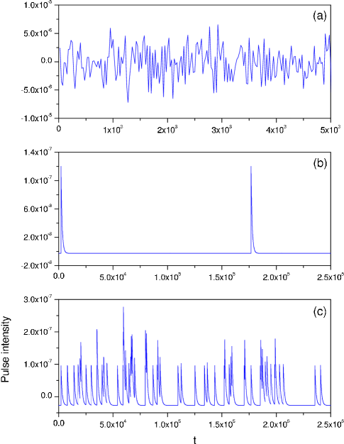
Figure 1: (a) Random noise function, $\delta R_{G}(t)$, corresponding to a Gaussian white noise with $\gamma=0.1\ \!\omega_{0}$ ($\omega_{0}=2.2049\times 10^{-4}$ a.u. is the harmonic frequency associated with the nonseparable adsorbate-substrate interaction potential (see section 3.1)). (b) Random noise function, $\delta R_{S}(t)$, corresponding to a shot noise with $\lambda=\gamma$. (c) Random noise function, $\delta R_{S}(t)$, corresponding to a shot noise with $\lambda=10\ \!\gamma$. The calculations refer to Na atoms at $T=200$ K and assuming $\lambda^{\prime}=10^{-3}$ a.u. (41.3 ps ^-1).

2.2.3 Relationship between coverage and the collision frequency

Here we would like to show how the coverage $\theta$ and $\lambda$ can be related in a simple manner. In the elementary kinetic theory of transport in gases [18] diffusion is proportional to the mean free path $\bar{l}$, which is proportionally inverse to both the density of gas particles and the effective area of collision when a hard-sphere model is assumed. For two-dimensional collisions the effective area is replaced by an effective length (twice the radius $\rho$ of the adparticle) and the gas density by the surface density $\sigma$. Accordingly, the mean free path is given by

$$\bar{l}=\frac{1}{2\sqrt{2}\rho\sigma}.$$ (37)

Taking into account the Chapman-Enskog theory for hard spheres, the self-diffusion coefficient can be written as

$$D=\frac{1}{6\rho\sigma}\ \!\sqrt{\frac{k_{B}T}{m}}.$$ (38)

Now, from Einstein’s relation (see section 2.2.4), and taking into account that $\theta=a^{2}\sigma$ for a square surface lattice of unit cell length $a$, we finally obtain

$$\lambda=\frac{6\rho}{a^{2}}\ \!\sqrt{\frac{k_{B}T}{m}}\ \!\theta.$$ (39)

Therefore, given a certain surface coverage and temperature, $\lambda$ can be readily estimated from equation (39). Notice that when the coverage is increased by one order of magnitude, the same holds for $\lambda$ at a given temperature.

2.2.4 Interacting adsorbate dynamics within the Langevin equation

Except for the case of a free-potential regime, the analytical study of particle motion in two dimensions results intractable in general due to the correlations between the two degrees of freedom. However, since we are interested in offering an analytical formulation that allows to better understand the process ruling surface diffusion and low vibrational motions, it is sufficient to proceed in one dimension and then try to adapt the resulting formulation to two dimensions. Thus, the motion of an adsorbate subjected to the action of a bath consisting of another adsorbates on a static one-dimensional surface potential can be well described by a generalized Langevin equation,

$$\ddot{x}(t)=-\int_{0}^{t}\eta(t-t^{\prime})\ \!\dot{x}(t^{\prime})\ \!dt^{\prime}+F(x(t))+\delta R(t),$$ (40)

where $x$ represents the adsorbate coordinate, and its first and second time derivatives are expressed by one and two dots on the $x$ variable, respectively. In this equation, $\eta(t)$ is the bath memory function, which includes the effects arising from both the Gaussian white noise and the shot noise. Thus, the noise source is expressed as the sum of both contributions,

$$\delta R_{GS}(t)=\delta R_{G}(t)+\delta R_{S}(t).$$ (41)

Regarding the deterministic term, $F=-\nabla V$ is the deterministic force per mass unit derived from the periodic surface interaction potential ($V(x)=V(x+a)$, $a$ being the period along the $x$ direction). If $\tau_{c}$ is relatively small (i.e., collision effects relax relatively fast), the memory function in equation (40) will be local in time. This allows to express the memory function as $\eta(t-t^{\prime})\simeq(\gamma+\lambda)\delta(t-t^{\prime})$ and expand the upper time limit in the integral to infinity. Taking into account this approximation and from the fluctuation-dissipation theorem, which leads to $\eta=\gamma+\lambda$, equation (40) becomes

$$\ddot{x}(t)=-\eta\dot{x}(t)+F(x(t))+\delta R_{G}(t)+\delta R_{S}(t).$$ (42)

The solutions of this equation can be straightforwardly obtained by formal integration, this rendering

$$v(t) = v_{0}e^{-\eta t}+\int_{0}^{t}e^{-\eta(t-t^{\prime})}F(x(t^{\prime}))\ \!dt^{\prime}+\int_{0}^{t}e^{-\eta(t-t^{\prime})}\delta R_{GS}(t^{\prime})\ \!dt^{\prime},$$ (43)

$$x(t) = x_{0}+\frac{v_{0}}{\eta}\ \!(1-e^{-\eta t})+\frac{1}{\eta}\int_{0}^{t}\Big{[}1-e^{-\eta(t-t^{\prime})}\Big{]}F(x(t^{\prime}))\ \!dt^{\prime}$$ (44)

$$+ \frac{1}{\eta}\int_{0}^{t}\Big{[}1-e^{-\eta(t-t^{\prime})}\Big{]}\delta R_{GS}(t^{\prime})\ \!dt^{\prime},$$

where $v_{0}=v(0)$ and $x_{0}=x(0)$. As can be seen, for $\delta R_{GS}=0$, equations (43) and (44) become the formal solutions of purely deterministic equations of motion. Therefore, without loss of generality, these solutions can be more conveniently expressed as

$$v(t) = v_{d}(t)+v_{s,G}(t)+v_{s,S}(t),$$ (45)

$$x(t) = x_{d}(t)+x_{s,G}(t)+x_{s,S}(t),$$ (46)

where $d$ refers to the deterministic terms and $s$ to those depending on the stochastic forces. Nonetheless, note that when $\delta R_{GS}(t)\neq 0$ the deterministic part will also present some stochastic features due to the evaluation of $F(x)$ along the trajectory $x(t)$, which is stochastic.

Taking advantage of equation (36), we can write

$$\langle v(t)\rangle = \bar{v}_{d}(t),$$ (47)

$$\langle v^{2}(t)\rangle = \bar{v}^{2}_{d}(t)+\langle v_{s,G}^{2}(t)\rangle+\langle v_{s,S}^{2}(t)\rangle,$$ (48)

$$\langle x(t)\rangle = \bar{x}_{d}(t),$$ (49)

$$\langle x^{2}(t)\rangle = \bar{x}^{2}_{d}(t)+\langle x_{s,G}^{2}(t)\rangle+\langle x_{s,S}^{2}(t)\rangle,$$ (50)

where the barred magnitudes indicate the respective averages of the deterministic part of the solutions, and

$$\langle v_{s,X}^{2}(t)\rangle = e^{-2\eta t}\int_{0}^{t}dt^{\prime}\ \!e^{2\eta t^{\prime}}\int_{-t^{\prime}}^{t-t^{\prime}}e^{\eta\tau}\mathcal{G}_{X}(\tau)\ \!d\tau,$$ (51)

$$\langle x_{s,X}^{2}(t)\rangle = \frac{1}{\eta^{2}}\int_{0}^{t}dt^{\prime}\ \!\Big{[}1-e^{-\eta(t-t^{\prime})}\Big{]}\int_{-t^{\prime}}^{t-t^{\prime}}\Big{[}1-e^{-\eta(t-t^{\prime}-\tau)}\Big{]}\ \!\mathcal{G}_{X}(\tau)\ \!d\tau,$$ (52)

with $X=G$ or $S$. For $X=G$, the final form of these expressions reads as

$$\langle v_{s,G}^{2}(t)\rangle = \frac{\gamma}{\eta}\frac{1}{\alpha^{2}}\ \!\Big{(}1-e^{-2\eta t}\Big{)}$$ (53)

$$\langle x_{s,G}^{2}(t)\rangle = \frac{\gamma}{\eta^{3}}\frac{1}{\alpha^{2}}\ \!\Big{[}2\eta t+1-\Big{(}2-e^{-\eta t}\Big{)}^{2}\Big{]},$$ (54)

and for $X=S$ as

$$\langle v_{s,S}^{2}(t)\rangle = \frac{1}{\alpha^{2}}\ \!\bigg{\{}\frac{\lambda}{\eta}\frac{\lambda^{\prime}}{(\lambda^{\prime}-\eta)}\ \!\Big{(}1-e^{-2\eta t}\Big{)}-\frac{2\lambda^{\prime}\lambda}{\lambda^{\prime 2}-\eta^{2}}\ \!\Big{[}1-e^{-(\lambda^{\prime}+\eta)t}\Big{]}\bigg{\}},$$ (55)

$$\langle x_{s,S}^{2}(t)\rangle = \frac{\lambda}{\eta^{3}}\frac{1}{\alpha^{2}}\ \!\bigg{\{}2\eta t-\frac{4\lambda^{\prime}-2\eta}{\lambda^{\prime}-\eta}\ \!\Big{(}1-e^{-\eta t}\Big{)}+\frac{2\lambda^{\prime}}{2(\lambda^{\prime}-\eta)}\ \!\Big{(}1-e^{-2\eta t}\Big{)}$$ (56)

$$+ \frac{2\eta^{2}}{\lambda^{\prime}(\lambda^{\prime}-\eta)}\ \!\Big{(}1-e^{-\lambda^{\prime}t}\Big{)}-\frac{2\eta^{2}}{\lambda^{\prime 2}-\eta^{2}}\ \!\Big{[}1-e^{-(\lambda^{\prime}+\eta)t}\Big{]}\bigg{\}}.$$

Introducing now the assumption $\lambda^{\prime}\gg\lambda$, we obtain

$$\langle v_{s,S}^{2}(t)\rangle \approx \frac{\lambda}{\eta}\frac{1}{\alpha^{2}}\ \!\Big{(}1-e^{-2\eta t}\Big{)},$$ (57)

$$\langle x_{s,S}^{2}(t)\rangle \approx \frac{\lambda}{\eta^{3}}\frac{1}{\alpha^{2}}\Big{[}2\eta t+1-\Big{(}2-e^{-\eta t}\Big{)}^{2}\Big{]}.$$ (58)

These equations are identical to equations (53) and (54), except for a weighting factor $\lambda/\eta$. The weighting factors $\gamma/\eta$ and $\lambda/\eta$ indicate the contribution arising from each noise. Adding equations (53) and (57), on the one hand, and equation (54) and (58), on the other hand, we reach

$$\langle v_{s}^{2}(t)\rangle \approx \frac{1}{\alpha^{2}}\ \!\Big{(}1-e^{-2\eta t}\Big{)},$$ (59)

$$\langle x_{s}^{2}(t)\rangle \approx \frac{1}{\eta^{2}}\frac{1}{\alpha^{2}}\Big{[}2\eta t+1-\Big{(}2-e^{-\eta t}\Big{)}^{2}\Big{]},$$ (60)

where no clue about the type of noise is left. Equation (59) can now be used to determine the value of $\alpha$; assuming that the equipartition theorem satisfies for $t\to\infty$,

$$\frac{1}{2}\ \!m\langle v^{2}(\infty)\rangle=\frac{1}{2}\ \!k_{B}T.$$ (61)

Therefore, since $\bar{v}^{2}_{d}(t)=\bar{v}^{2}_{0}e^{-2\eta t}$ and the time-dependent term in equation (59) vanishes asymptotically,

$$\alpha=\sqrt{\frac{m}{k_{B}T}}.$$ (62)

If the system is initially thermalized (i.e., it follows a Maxwell-Boltzmann distribution in velocities) and has a uniform probability distribution in positions around $x=0$, then $\bar{v}_{0}=0$, $\bar{v}^{2}_{0}=k_{B}T/m$ and $\bar{x}_{0}=0$. Thus, for $\lambda^{\prime}\gg\lambda$ (i.e., in the limit of a Poissonian white noise), we finally obtain

$$\langle v(t)\rangle = 0,$$ (63)

$$\langle v^{2}(t)\rangle = \frac{k_{B}T}{m},$$ (64)

$$\langle x(t)\rangle = 0,$$ (65)

$$\langle x^{2}(t)\rangle = \bar{x}_{0}^{2}+\frac{k_{B}T}{m\eta^{2}}\ \!\Big{[}2\eta t+1-\Big{(}2-e^{-\eta t}\Big{)}^{2}\Big{]}.$$ (66)

Obviously, these equations constitute a limit and therefore for values of the parameters out of the range of the approximation deviations will be apparent.

As happens with Brownian motion, two regimes are clearly distinguishable from equation (66). For $\eta t\ll 1$ collision events are rare and the adparticle shows an almost free motion with relatively long mean free paths. This is the ballistic or free-diffusion regime, characterized by

$$\langle x^{2}(t)\rangle\sim\frac{k_{B}T}{m}\ \!t^{2}.$$ (67)

On the other hand, for $\eta t\gg 1$ there is no free diffusion since the effects of the stochastic force (collisions) are dominant. This is the diffusive regime, where mean square displacements are linear with time:

$$\langle x^{2}(t)\rangle\sim\frac{2k_{B}T}{m\eta}\ \!t=2Dt\ \!.$$ (68)

This is the so-called Einstein’s law. Note from equation (68) that: (1) lowering the friction $\eta$ acting on the adparticle leads to a faster diffusion (the diffusion coefficient $D$ increases) and (2) diffusion becomes more active when the surface temperature increases.

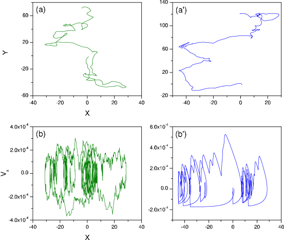
Figure 2: Upper panels: Trajectory dynamics for $V(x,y)=0$ and: (a) a Gaussian white noise with $\gamma=0.1\ \!\omega_{0}$ ($\omega_{0}=2.2049\times 10^{-4}$ a.u.) and (a’) a shot noise with $\lambda=\gamma$. Lower panels: Phase diagram corresponding to the trajectories represented above. The trajectories have been propagated for 2.5$\times$10⁶ a.u. and $\lambda^{\prime}=10^{-3}$ a.u.

To conclude this section, it is worth comparing the type of dynamics ruled by each noise, Gaussian or shot. In figures 2 and 3 we present some trajectories together with their phase diagram (for the $x$-coordinate) for $V(x,y)=0$ and $V(x,y)$ as given by equation (98) (see section 3), respectively. The noise functions are such that $\lambda=\gamma$ (figures 1(a) and 1(b)) and the numerical details are the same as in figure 1 (the total propagation time is $t=2.5\times 10^{6}$ a.u.). The first striking difference that we can appreciate is that, because of the continuous kicking in the case of a Gaussian white noise, the trajectory looks much smoother in the case of a shot noise. This can be better seen in the upper panels of figure 3 —the effect is not so pronounced in figure 2 because we have only represented one out of 50 time steps— and also in the lower panels of both figures. The lack of smoothness in the trajectories affected by the Gaussian white noise is a manifestation of this type of kicking (see figure 1(a)). On the other hand, it is also interesting to observe the difference in the dynamics induced in both cases when a potential is introduced. The presence of potential wells, where a particle can remain trapped, will make the particle to undergo a vibrational motion inside such wells. The low frequency vibrational motion observed gives rise to the so-called frustrated translational mode or T mode.

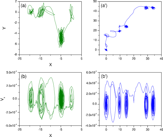
Figure 3: Upper panels: Trajectory dynamics for $V(x,y)$ as given by model 3 (see section 3.1) and: (a) a Gaussian white noise with $\gamma=0.1\ \!\omega_{0}$ and (a’) a shot noise with $\lambda=\gamma$. Lower panels: Phase diagram corresponding to the trajectories represented above. The trajectories have been propagated for 2.5$\times$10⁶ a.u. and $\lambda^{\prime}=10^{-3}$ a.u.

2.2.5 The velocity autocorrelation function

The average magnitudes given in section 2.2.4 are only relevant to understand the ensemble behaviour of the trajectories along time, and therefore to have some idea on the dynamics induced by the corresponding interaction potential. In order to get a deeper insight into the diffusion process —and therefore also into the line shapes associated with the dynamic structure factor— it is important first to compute the velocity autocorrelation function given by equation (10). This function can be expressed as

$$\mathcal{C}(\tau)=\langle v_{\Delta{\bf K}}(t)\ \!v_{\Delta{\bf K}}(t+\tau)\rangle=e^{-2\eta t-\eta\tau}\int_{0}^{t}dt^{\prime}\ \!e^{2\eta t^{\prime}}\int_{-t^{\prime}}^{t+\tau-t^{\prime}}e^{\eta s}\mathcal{G}_{GS}(s)\ \!ds.$$ (69)

As seen, this expression only depends on the stochastic part of the solution for the velocity; the deterministic one cancels out in the averaging procedure. Moreover, it also takes into account that there are no correlations among the two space coordinates ($x$ and $y$). This is true in any case for the Gaussian white noise; for the shot noise it only holds in the white noise limit, otherwise some correlations among the two degrees of freedom could still be present when $V\neq 0$ due to the finite duration of the pulses. To avoid this inconvenience, which deviates the treatment from analyticity, here we assume conditions for which the white noise limit is satisfied (see section 2.2.4). Finally, note that in equation (69) it is also considered that the motion along both coordinates contribute equally (i.e., $\langle v_{x}(0)\ \!v_{x}(t)\rangle\approx\langle v_{y}(0)\ \!v_{y}(t)\rangle$). This finds its justification in the fact that the potential models that will be used display the same symmetry along each direction and therefore the corresponding dynamics is expected to be the same (this would not be the case, for example, when the activation barrier is much higher in one direction). In this sense, the calculation of the velocity autocorrelation function can be regarded as one-dimensional.

The analytical results derived following the assumptions described above will be compared with the numerical simulations, which have been obtained using the corresponding exact expressions (e.g., the r.h.s. of the first equality in equation (8)). In order to better interpret our exact numerical results two limiting cases will be studied below. It is precisely the discussion in terms of both cases what will allow us to better understand the physical processes taking place on the surface.

2.2.6 The low corrugation regime. Quasi-free adparticles.

In the case of diffusion on low corrugated surfaces, where the role of the adiabatic adsorbate-substrate interaction potential is negligible and only the action of the thermal phonons is relevant, one can assume $V\approx 0$. The adparticle motion can then be regarded as quasi-free since it is not ruled by a potential, but only influenced by the stochastic forces. Within this regime, equation (69) becomes

$$\mathcal{C}(\tau)=\frac{\gamma}{\eta}\frac{k_{B}T}{m}\ \!e^{-\eta\tau}+\frac{\lambda}{\eta}\frac{k_{B}T}{m}\frac{\lambda^{\prime 2}}{\lambda^{\prime 2}-\eta^{2}}\left(e^{-\eta\tau}-\frac{\eta}{\lambda^{\prime}}\ \!e^{-\lambda^{\prime}\tau}\right).$$ (70)

In this expression the contributions arising from each noise source are apparent. However, in the limit of Poissonian white noise ($\lambda^{\prime}\gg\lambda$) such a distinction disappears; under such a condition equation (70) becomes

$$\mathcal{C}(\tau)=\frac{k_{B}T}{m}\ \!e^{-\eta\tau}.$$ (71)

Unless the relaxation of the collisional effects is relevant, these effects and those caused by the surface should be indistinguishable and equation (71) would describe accurately the loss of correlation, with $\tilde{\tau}$ given in terms of $\eta$ rather than $\gamma$ and/or $\lambda$ separately.

The expression for the intermediate scattering function resulting from equation (71) is

$$I(\Delta K,t)=\exp\left[-\chi^{2}\left(e^{-\eta t}+\eta t-1\right)\right],$$ (72)

where the so-called shape parameter $\chi$ [30, 31] is defined as

$$\chi^{2}\equiv\langle v_{0}^{2}\rangle\Delta K^{2}/\eta^{2}.$$ (73)

From this relation we can obtain both the mean free path $\bar{l}\equiv\tilde{\tau}\sqrt{\langle v_{0}^{2}\rangle}$ and the self-diffusion coefficient $D\equiv\tilde{\tau}\langle v_{0}^{2}\rangle$ (Einstein’s relation). When the coverage increases, the collisions among adsorbates also increase, and so $\lambda$ (see section 2.2.4) and therefore $\eta$. As can be easily shown, equation (72) displays a Gaussian decay at short times that does not depend on the particular value of $\eta$, while at longer times it decays exponentially with a rate given by $\eta^{-1}$. Thus, with $\eta$, the decay of the intermediate scattering function becomes slower. The type of decay is important concerning the width and the shape of the dynamic structure factor [12, 30].

The above described effects can be quantitatively understood by means of the expression of the dynamic structure factor obtained analytically from equation (72),

$$S(\Delta K,\omega) = \frac{e^{\chi^{2}}}{\pi\eta}\ \!\chi^{-2\chi^{2}}\ \!{\rm Re}\left\{\chi^{-2i\omega/\eta}[\tilde{\Gamma}(\chi^{2}+i\omega/\eta)-\tilde{\Gamma}(\chi^{2}+i\omega/\eta,\chi^{2})]\right\}$$ (74)

$$= \frac{e^{\chi^{2}}}{\pi}\sum_{n=0}^{\infty}\frac{(-1)^{n}\chi^{2n}}{n!}\frac{(\chi^{2}+n)\eta}{\omega^{2}+[(\chi^{2}+n)\eta]^{2}}\ \!.$$

Here, the $\tilde{\Gamma}$ symbol in the first line denotes both the Gamma and incomplete Gamma functions (depending on the corresponding argument), respectively. As can be noted in the high friction limit, equation (74) becomes a Lorentzian function, its full width at half maximum (FWHM) being $\Gamma=2\eta\chi^{2}$, which approaches zero as $\eta$ increases (narrowing effect). This in sharp contrast to what one could expect — as the frequency between successive collisions increases one would expect that the line shape gets broader (effect of the pressure in the spectral lines of gases). The physical reason for this effect could be explained as follows. As $\eta$ increases the particle’s mean free path decrease and therefore correlations are lost more slowly. In the limit case where friction is such that the particle remains in the same place, the van Hove function becomes a $\delta$-function, the intermediate scattering function remains equal to 1 and the dynamic structure factor consists of a $\delta$-function at $\omega=0$. Conversely, in the low friction limit the line shape is given by a Gaussian function, whose width is $\Gamma=2\sqrt{2\ln 2}\sqrt{k_{B}T/m}\ \!\Delta K$, which does not depend on $\eta$. This is the case for a two–dimensional free gas [30, 32]. This gradual change of the line shapes as a function of the friction and/or the parallel momentum transfer leading to a change of the shape parameter $\chi$ is known as the motional narrowing effect [11, 12, 30]. Note that in our approach the friction is related to the coverage. Thus, at higher coverages a narrowing effect is predicted for a flat surface [15].

2.2.7 The harmonic oscillator. Bound adparticles.

In contrast with the case of a dynamics where $V$ does not play a relevant role, we can devise a particle fully trapped within a potential well. The harmonic oscillator is an appropriate working model to understand the physics associated with this problem. This model also allows us to understand the behaviour associated with the T mode, which comes precisely from the oscillating behaviour undergone by the particle when the diffusional motion is temporarily frustrated.

For a harmonic oscillator, the behaviour of the adparticle becomes very apparent when looking at the corresponding velocity autocorrelation function, which reads [12, 34] as

$$\mathcal{C}(\tau)=\frac{k_{B}T}{m}\ \!e^{-\eta\tau/2}\left(\cos\bar{\omega}\tau-\frac{\eta}{2\bar{\omega}}\sin\bar{\omega}\tau\right).$$ (75)

Here,

$$\bar{\omega}\equiv\sqrt{\omega_{0}^{2}-\frac{\eta^{2}}{4}},$$ (76)

$\omega_{0}$ being the harmonic frequency. Alternatively, equation (75) can also be recast as

$$\mathcal{C}(\tau)=\frac{k_{B}T}{m}\ \!\frac{\omega_{0}}{\bar{\omega}}\ \!e^{-\eta\tau/2}\cos(\bar{\omega}\tau+\delta),$$ (77)

with

$$\delta\equiv(\tan)^{-1}\left(\frac{\eta/2}{\bar{\omega}}\right).$$ (78)

Note that equation (71) can be easily recovered after some algebra in the limit $\omega_{0}\to 0$ from either equation (75) or (77). In the case of anharmonic potentials, provided that we work within an approximate harmonic regime, $\omega_{0}$ would represent the corresponding approximate harmonic frequency.

The only information about the structure of the lattice is found in the shape parameter through $\Delta K$ [see equation (73)]. When large parallel momentum transfers are considered, both the periodicity and the structure of the surface have to be taken into account. Consequently, the shape parameter should be changed for different lattices. The simplest model including the periodicity of the surface is that developed by Chudley and Elliott [33], who proposed a master equation for the pair-distribution function in space and time assuming instantaneous discrete jumps on a two-dimensional Bravais lattice. Very recently, a generalized shape parameter based on that model has been proposed to be [31]

$$\chi_{l}(\Delta{\bf K})\equiv\sqrt{\frac{\Gamma_{\nu}(\Delta{\bf K})}{2\eta}},$$ (79)

where, for our approach, it has been written $\eta$ instead of $\gamma$. Here, $\Gamma_{\nu}(\Delta{\bf K})$ represents the inverse of the correlation time and is expressed as

$$\Gamma_{\nu}(\Delta{\bf K})=\nu\sum_{\bf j}P_{\bf j}\ \![1-\cos({\bf j}\cdot\Delta{\bf K})],$$ (80)

$\nu$ being the total jump rate out of an adsorption site and $P_{\bf j}$ the relative probability that a jump with a displacement vector ${\bf j}$ occurs.

Introducing now equation (77) into (9) leads to the following expression for the intermediate scattering function

$$I(\Delta K,t)=\exp\left\{-\frac{\chi_{l}^{2}\eta^{2}}{\bar{\omega}\omega_{0}}\left[\cos\delta-e^{-\eta t/2}\cos(\bar{\omega}t-\delta)\right]\right\}.$$ (81)

The argument of this function displays an oscillatory behaviour around a certain value with the amplitude of the oscillations being exponentially damped. This translates into an also decreasing behaviour of the intermediate scattering function, which also displays oscillations around the asymptotic value. This means that after relaxation the intermediate scattering function has not fully decayed to zero unlike the free-potential case. Again, in the limit $\omega_{0}\to 0$, equation (81) approaches equation (72).

In order to obtain an analytical expression for the dynamic structure factor, it is convenient to express equation (81) as

$$I(\Delta K,t) = e^{-\chi_{l}^{2}f(\bar{\omega},t)}$$ (82)

$$= e^{-\chi_{l}^{2}A_{1}}\sum_{m,n=0}^{\infty}\frac{(-1)^{m+n}}{m!\ \!n!}\ \!\chi_{l}^{2(m+n)}A_{3}^{m}A_{4}^{n}$$

$$\qquad\qquad\qquad\times e^{i(m-n)\delta}e^{-(m+n)\eta t/2}e^{i(m-n)\bar{\omega}t},$$

where

$$f(\bar{\omega},t)\equiv A_{1}+A_{3}e^{i\delta}e^{-(\eta/2-i\bar{\omega})t}+A_{4}e^{-i\delta}e^{-(\eta/2+i\bar{\omega})t},$$ (83)

with

$$A_{1} = \frac{\omega_{0}}{\bar{\omega}}\frac{\eta^{2}\{2(\eta/2)\bar{\omega}\sin\delta+[\bar{\omega}^{2}-(\eta/2)^{2}]\cos\delta\}}{[(\eta/2)^{2}+\bar{\omega}^{2}]^{2}},$$ (84)

$$A_{3} = \frac{\omega_{0}}{\bar{\omega}}\frac{\eta^{2}}{2(\eta/2-i\bar{\omega})^{2}},$$ (85)

$$A_{4} = \frac{\omega_{0}}{\bar{\omega}}\frac{\eta^{2}}{2(\eta/2+i\bar{\omega})^{2}},$$ (86)

where the coefficients $A_{i}$ has been put in terms of $\eta$, $\bar{\omega}$ and $\delta$. From equation (82), it is now straightforward to derive an expression for the dynamic scattering factor, which results

$$S(\Delta K,\omega) = \frac{e^{-\chi_{l}^{2}A_{1}}}{\pi}\sum_{m,n=0}^{\infty}\frac{(-1)^{m+n}}{m!\ \!n!}\ \!\chi_{l}^{2(m+n)}A_{3}^{m}A_{4}^{n}e^{i(m-n)\delta}$$ (87)

$$\qquad\qquad\times\frac{(m+n)\eta/2}{[\omega-(m-n)\bar{\omega}]^{2}+[(m+n)\eta/2]^{2}}.$$

For a harmonic oscillator, there is no diffusion and, therefore, equation (87) is only valid when $m\neq n$. All the Lorentzian functions contributing to equation (87) are due to the creation and annihilation events of the T mode. These Lorentzians are characterized by a width given by $\Gamma=(m+n)\eta/2$, which increases with $\eta$. This broadening (proportional to $\eta$) undergone by the dynamic structure factor is thus contrary to the narrowing effect observed in the case of a flat surface. It can be assigned to the confined or bound motion displayed by the particle ensemble when trapped inside the potential wells. Hence, in order to detect broadening of the line shapes in surface diffusion experiments, adparticles must spend some time confined inside potential wells, since the broadening will be induced by the presence of temporary vibrational motions.

2.2.8 General periodic surface potentials. Temporary trapped adparticles.

As seen above, the broadening of the diffusion line shapes is provoked by the temporary trapping. To demonstrate this assertion here we are going to consider a general velocity autocorrelation function which keeps the functional form of equation (77), but whose parameters do not hold the same relations as those characterizing a harmonic oscillator [12]. That is,

$$\mathcal{C}(t)=\frac{k_{B}T}{m}\ \!e^{-\tilde{\eta}\tau}\cos(\tilde{\omega}t+\tilde{\delta}),$$ (88)

where the values of the parameters $\tilde{\eta}$, $\tilde{\omega}$ and $\tilde{\delta}$ are obtained from a fitting to the numerical results —there is no any relation among them as in the case of the harmonic oscillator model. From equation (88) one easily reaches the corresponding expression for the intermediate scattering function,

$$I(\Delta K,t) = e^{-\chi_{l}^{2}\tilde{f}(\tilde{\omega},t)}$$ (89)

$$= e^{-\chi_{l}^{2}\tilde{A}_{1}-\chi_{l}^{2}\tilde{A}_{2}t}\sum_{m,n=0}^{\infty}\frac{(-1)^{m+n}}{m!\ \!n!}\ \!\chi_{l}^{2(m+n)}\tilde{A}_{3}^{m}\tilde{A}_{4}^{n}$$

$$\qquad\qquad\qquad\times e^{i(m-n)\tilde{\delta}}e^{-(m+n)\tilde{\eta}t}e^{i(m-n)\tilde{\omega}t},$$

which is analogous to equation (82). In equation (89),

$$\tilde{f}(\tilde{\omega},t)\equiv\tilde{A}_{1}+\tilde{A}_{2}t+\tilde{A}_{3}e^{i\tilde{\delta}}e^{-(\tilde{\eta}-i\tilde{\omega})t}+\tilde{A}_{4}e^{-i\tilde{\delta}}e^{-(\tilde{\eta}+i\tilde{\omega})t},$$ (90)

and

$$\tilde{A}_{1} = \frac{\tilde{\eta}^{2}[2\tilde{\eta}\tilde{\omega}\sin\tilde{\delta}+(\tilde{\omega}^{2}-\tilde{\eta}^{2})\cos\tilde{\delta})}{(\tilde{\eta}^{2}+\tilde{\omega}^{2})^{2}},$$ (91)

$$\tilde{A}_{2} = \frac{\tilde{\eta}^{2}(\tilde{\eta}\cos\tilde{\delta}-\tilde{\omega}\sin\tilde{\delta})}{\tilde{\eta}^{2}+\tilde{\omega}^{2}},$$ (92)

$$\tilde{A}_{3} = \frac{\tilde{\eta}^{2}}{2(\tilde{\eta}-i\tilde{\omega})^{2}},$$ (93)

$$\tilde{A}_{4} = \frac{\tilde{\eta}^{2}}{2(\tilde{\eta}+i\tilde{\omega})^{2}}.$$ (94)

Unlike the case of the harmonic oscillator, notice now that there is a linear dependence on time in $\tilde{f}$ because of the independence of $\tilde{\eta}$, $\tilde{\omega}$ and $\tilde{\delta}$. This leads to an exponentially decaying factor in equation (89), which accounts for the diffusion and that makes the intermediate scattering function to vanish at asymptotic times. In this sense, the intermediate scattering function can be considered as containing both phenomena, diffusion and low vibrational motions. This effect is better appreciated in the dynamic structure factor,

$$S(\Delta K,\omega) = \frac{e^{-\chi_{l}^{2}\tilde{A}_{1}}}{\pi}\sum_{m,n=0}^{\infty}\frac{(-1)^{m+n}}{m!\ \!n!}\ \!\chi_{l}^{2(m+n)}\tilde{A}_{3}^{m}\tilde{A}_{4}^{n}e^{i(m-n)\delta}$$ (95)

$$\qquad\times\frac{\chi_{l}^{2}\tilde{A}_{2}+(m+n)\tilde{\eta}}{[\omega-(m-n)\tilde{\omega}]^{2}+[\chi^{2}\tilde{A}_{2}+(m+n)\tilde{\eta}]^{2}}.$$

This general expression clearly shows that both motions (diffusion and oscillatory) cannot be separated at all. The Q–peak is formed by contributions where $m=n$, for which each partial FWHM is given by

$$\Gamma_{Q}=\chi_{l}^{2}\tilde{A}_{2}+2\,m\,\tilde{\eta}.$$ (96)

Analogously, the T–peaks come from the sums with $n\neq m$ and each partial FWHM is given by

$$\Gamma_{T}=\chi_{l}^{2}\tilde{A}_{2}+(m+n)\,\tilde{\eta}.$$ (97)

If the Gaussian approximation is good enough, the value of $\tilde{\eta}$ will not be too different from the nominal value of $\eta$ and, therefore, both peaks will display broadening as $\eta$ increases. This is a very remarkable result since a relatively simple model, as the one described here, can explain the corresponding experimental broadenings observed with coverage. Thus, broadening arises from the temporary confinement of the adparticles inside potential wells along their motion on the surface [15]. The problem of the experimental deconvolution has been already discussed elsewhere [31]. Here we would like only to mention that using this simple model, such deconvolutions would be more appropriate in order to extract useful information about diffusion constants and jump mechanisms. Finally, as mentioned before, the motional narrowing effect will govern the gradual change of the whole line shape as a function of the friction or, equivalently, the coverage, the parallel momentum transfer and the jump mechanism.

3 Results

For a better understanding of the concepts introduced in section 2, here we present results for two different types of two-dimensional surfaces: flat and corrugated. Since much research has been developed for Na atoms adsorbed on a Cu(001) surface, we will carry out our numerical simulations taking into account the periodic, separable corrugated potential found in the literature for this system (see, for example, reference [7]).

3.1 Computational details

As in reference [7], we have considered two values of the coverage in our calculations, $\theta=0.028$ and 0.18, where $\theta_{Na}=1$ corresponds to one Na atom per Cu(001) surface atom —or, equivalently, $\sigma=1.53\times 10^{19}$ atom/cm² [8]. All the friction coefficients are given in atomic units. Taking into account the values $a=2.557$ Å and $\rho=2$ Å for the unit cell length and the Na atomic radius, and using equation (39), the values of $\lambda$ associated with the coverages used here are $\lambda=3.34\times 10^{-6}$ a.u. for $\theta=0.028$ and $\lambda=2.15\times 10^{-5}$ a.u. for $\theta=0.18$ at $T=200$ K. For the surface friction we have considered the value also given in the literature [7], $\gamma=0.1\ \!\omega_{0}=2.2049\times 10^{-5}$ a.u., where $\omega_{0}$ is the harmonic frequency associated with the periodic surface potential (see section 3.3). With these two frictions ($\lambda$ and $\gamma$) the resulting total friction is $\eta\approx 2.53\times 10^{-5}$ a.u. for $\theta=0.028$ and $\eta\approx 4.35\times 10^{-5}$ a.u. for $\theta=0.18$. Regarding the collision relaxation rate, we have assumed $\lambda^{\prime}=10^{-3}$ a.u., which allows us to use the standard Langevin equation with a white shot noise. As far as we know, no information about that parameter is found in the literature and therefore the interacting single adsorbate approximation could also give us an estimation of the duration of the adsorbate-adsorbate collision. Finally, the Verlet algorithm [35] is used to solve the corresponding Langevin equation.

3.2 Flat surface model. The low corrugation regime

First we analyze the case of adsorbate diffusion on a flat surface, i.e., the case of a two-dimensional gas [30, 32]. This example is representative of low corrugated surfaces, where the role of the activation barrier is negligible.

As seen in section 2.2.4, when $V=0$, the dynamical magnitude $\langle x^{2}(t)\rangle$ displays two different dynamical regimes: ballistic ($t\ll 1/\eta$) and diffusive ($t\gg 1/\eta$). This can be seen in figure 4(a), where $\langle x^{2}(t)\rangle$ is effectively proportional to $t$ in the long time regime and depends on $t^{2}$ at short times (of the order of $1/\eta$). In the linear regime, the slope of $\langle x^{2}(t)\rangle$ increases as $\eta$ decreases, i.e., in accordance with Einstein’s law (see equation (68)), the diffusion decreases with the friction. By fitting the linear part of the graphs (dotted lines) to equation (68), we get $D=6.045\times 10^{-4}$ a.u. for $\theta=0.028$ and $D=3.510\times 10^{-4}$ a.u. for $\theta=0.18$. Note that these diffusion coefficients are not only related to the friction due to the surface (i.e., the adsorbate-substrate coupling), but also to the collisions among adsorbates. Indeed, we can see that for a given surface friction, the diffusion is inhibited by such collisions —it decreases with the coverage. This is a very remarkable result since in real experiments the surface friction is fixed and diffusion can then be studied taking only into account the coverage of the surface. On the other hand, from these values for $D$ we obtain, respectively, $\eta=2.50\times 10^{-5}$ a.u. and $\eta=4.35\times 10^{-5}$ a.u., which are in a good agreement with those used in our calculations (see section 3.1). This agreement between the simulation and the analytical model is particularly important because it validates our standard Langevin description.

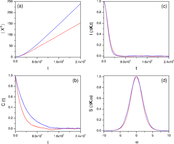
Figure 4: Dynamical magnitudes for two different values of the coverage, $\theta=0.028$ (blue) and $\theta=0.18$ (red): (a) $\langle x^{2}(t)\rangle$, (b) $\mathcal{C}(t)$, (c) $I(\Delta{\bf K},t)$ and (d) $S(\omega)$, with $\Delta K=1.23$ Å^-1. Dotted lines are the numerical fittings to the corresponding analytical formulas given in section 2.

The effect of the collisions also produces an important effect on the velocity autocorrelation function, $\mathcal{C}(t)$, plotted in Fig. 4(b). As seen, as $\theta$ increases this function decays faster. In particular, from the fitting of these results to equation (71) (normalized to unity) we have obtained $\eta\approx 2.52\times 10^{-5}$ a.u. for $\theta=0.028$ and $\eta\approx 4.32\times 10^{-5}$ a.u. for $\theta=0.18$, which again show a good agreement with the actual values employed in our simulations. This fast decay also indicates that higher order correlations (e.g., correlations at three or four times) will decay much faster. Their effect will be then negligible on the intermediate scattering function, thus validating the use of the Gaussian approximation, since such higher order correlations will not be relevant when passing from equation (8) to (9). The validity of the Gaussian approximation can be seen more explicitly when comparing the intermediate scattering functions obtained from the calculations with that fitted using equation (72). These results are plotted in figure 4(c) for $\Delta K=1.23$ Å^-1, where the fitting has been carried out with the values of $\eta$ used in the simulation and considering $\chi$ as the fitting parameter. We observe that not only the correspondence between the simulations and the analytical formulas are excellent from the figure, but also from the fitted values of $\chi$: $\chi_{fit}=3.16$ vs $\chi_{sim}=3.16$ for $\theta=0.028$, and $\chi_{fit}=1.81$ vs $\chi_{sim}=1.83$ for $\theta=0.18$. Notice that in agreement with equation (72), $I(t)$ displays an initial Gaussian falloff at short times, while for longer times its decay is exponential. Moreover, as also expected from equation (72), and equation (73), as the coverage increases a slower decay is observed.

Finally, in figure 4(d) we have plotted the dynamic structure factor after time Fourier transforming the intermediate scattering function obtained from both the numerical calculations and their corresponding analytical fittings. Note that, a narrowing of the Q peak is predicted with the coverage [15]. Regarding the shape of this peak, it can be shown that it is a mixture of Gaussian and Lorentzian functions. The Gaussian behaviour is ruled by the short time limit of the intermediate scattering function, while the Lorentzian behaviour arises from the long time exponential decay. The shape of the Q peak will depend on which of the two extreme regimes is dominant (motional narrowing effect) [12]. This analysis should be carried out when experimental results are deconvoluted [30] since it is very common to see fittings of the Q peak to a pure Lorentzian function.

3.3 Periodic, corrugated surface model

Now we are going to study the case of a periodic surface model described by the potential

$$V(x,y)=V_{0}\left[2-\cos(2\pi x/a)-\cos(2\pi y/a)\right],$$ (98)

with $a=2.557$ Å and $V_{0}=37.32$ meV. In this case, the surface corrugation is relatively strong and cannot be neglected, thus inducing important effects in the adsorbate dynamics. These effects can be well understood by using the third model described in section 2.2.8.

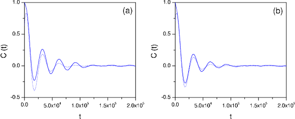
Figure 5: Velocity autocorrelation function, $\mathcal{C}(t)$, for two different values of the coverage: (a) $\theta=0.028$ and (b) $\theta=0.18$. Solid lines denote the numerical results obtained from the simulations and dotted lines the fittings to equation (88).

After figures 5, the diffusive and trapped regimes that appear under the presence of the surface corrugation give rise to the oscillating behaviour of the velocity autocorrelation function. The adparticles trapped inside the potential wells give rise to the oscillations, while the exponential damping arises as a consequence of the loss of correlation with time of both the particles moving outside the wells and those trapped inside. This behaviour thus approaches that described by equation (88), as seen from the fittings (dotted line) with parameters $\tilde{\eta}=5.13\times 10^{-5}$ a.u., $\tilde{\omega}=2.14\times 10^{-4}$ a.u. and $\tilde{\delta}=-0.874$ for $\theta=0.028$ (see figure 5(a)), and $\tilde{\eta}=5.96\times 10^{-5}$ a.u., $\tilde{\omega}=2.05\times 10^{-4}$ a.u. and $\tilde{\delta}=-0.776$ for $\theta=0.18$ (see figure 5(b)). Note that, since we have contributions from running and trapped or bound trajectories, here the fitting is not so good as that seen in section 3.2 for $V=0$. Recently, it has been shown [15] that if the velocity autocorrelation function is expressed as a linear combination of the corresponding functions for free particle and anharmonic oscillator, the fitting is highly improved. Obviously, the Gaussian approximation is no longer valid due to the presence of the corrugated potential. Nonetheless, it is important to stress that the model given by equation (88) is still valid to interpret the results obtained; not only the fitted parameters are of the order of those employed in the calculations, but they also follow the trend that one might expect from the exact ones. That is, as $\tilde{\eta}$ increases the exponential damping in $\mathcal{C}(t)$ is stronger and a slight shift of the oscillations is observed.

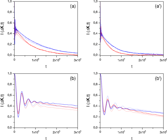
Figure 6: Intermediate scattering function for $\Delta K=1.23$ Å^-1 and two different values of the coverage: $\theta=0.028$ in panels (a) and (a’) along two directions, [110] and [100] and $\theta=0.18$ in panels (b) and (b’) along the same two directions. In the bottom panels observe details of the short time regime. Solid lines denote the numerical results obtained from the simulations and dotted lines the fittings to equation (89).

As seen in figure 6, the effects of the trapping or bound motion are also apparent in the intermediate scattering function, which is plotted for $\Delta K=1.23$ Å^-1, along two different directions and two coverages: panels (a) and (a’) for $\theta=0.028$ along the [110] and [100] directions, respectively; and panels (b) and (b’) for $\theta=0.18$ and along the same two directions. Note first that again here we can distinguish two decay regimes (which are present along both directions). The long time regime in the upper panels is characterized by an exponential damping, as in the case for $V=0$, which is typical of diffusion and will give rise to a predominance of the Lorentzian-like behaviour in the dynamic structure factor (see below). On the other hand, the short time regime in the bottom panels clearly shows the damped oscillating behaviour of $\mathcal{C}(t)$. These oscillations at short times will give rise to the T-mode peaks associated with the low frequency vibrational motions induced by the potential wells in the trapped trajectories. Moreover, the oscillating behaviour is more patent with the coverage giving rise to an inversion in the behaviour of the long time tail of $I(t)$. Unlike the intermediate scattering function associated with a flat surface dynamics, this faster decay with coverage will lead to a broadening of the Q peak in the dynamic structure factor. Moreover, also notice that the timescales ruling the decay are about two orders of magnitude larger than in the case with $V=0$. This is due to the presence of the potential, which allows to keep the phase correlation in equation (8) for longer times due to the trapping inside the potential wells [15].

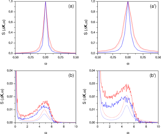
Figure 7: Dynamic structure factor for $\Delta K=1.23$ Å^-1 and two different values of the coverage: $\theta=0.028$ in panels (a) and (a’) along two directions, [110] and [100] and $\theta=0.18$ in panels (b) and (b’) along the same two directions. In the bottom panels observe details of the peaks corresponding to the T mode. Solid lines denote the numerical results obtained from the simulations and dotted lines the time Fourier transform of the fittings to equation (89).

Regarding the dynamic structure factor, displayed in figure 7 (as before, the four panels correspond to the same coverages and directions as in figure 6), the presence of the potential has three important differences with respect to the flat surface case. First, the trapping trajectories due to the surface corrugation give rise to the appearance of two symmetric peaks around the Q peak, the T-mode peaks which are located at $-5$ meV and 5 meV, approximately (in the lower panels of figure 7 only the right peak is showed); these peaks broadens with coverage. Second, the faster decay of $I(t)$ as the coverage increases translates into a broadening of the Q peak, which is in accordance to what one can observe experimentally [7]. Third, the Q peak is narrower than the corresponding in the flat surface case, around two orders of magnitude. This narrowing is due to the inhibition of the diffusive motion induced by the corrugation of the potential (a large number of particles get trapped inside the wells). In any case, the diffusion coefficient is governed by the Einstein relation and therefore decreases with the coverage.

Finally, it is worth stressing that there is a strong correlation between diffusion and low frequency vibrational motions [12]. This fact is easily appreciated in the two bottom panels of figure 7, where a strong overlapping of the two peaks is noticeable. In the Gaussian approximation, this overlapping can be understood from equation (95). In general, in order to extract the width of the Q and T peaks, experimentalists usually follows a deconvolution procedure where an effective Lorentzian function is assumed for each peak independently. After the study presented here (as well as in references [12, 31] within the single adsorbate approximation), this deconvolution procedure could lead to inconsistencies when extracting information because both peaks are strongly overlapped. Indeed, it can be shown [36] that depending on the parallel momentum transfer $\Delta{\bf K}$ considered, the overlapping of both peaks may become so strong that the Lorentzian fitting procedure would not be valid anymore. In the light of this study we propose a more general fitting procedure based on equation (95).

4 Conclusions

In this work, we have presented a full stochastic description of surface diffusion and low frequency vibrational motion for adsorbate/substrate systems with increasing coverages. A Langevin equation is used to describe the adparticle dynamics, where a Gaussian white noise simulates the effects of adsorbate-substrate friction and a white shot noise is used for the adsorbate-adsorbate interactions within what we call the interacting single adsorbate approximation. As shown, this theoretical stochastic framework not only provides a simple and complementary view of the processes taking place on a surface, but also explains the experimental observations, i.e., the line shape broadening of the Q peak ruling the diffusion process as a function of the coverage. The idea of replacing the dipole-dipole interaction by a white shot noise turns out to be crucial because for long time processes, as the diffusion one, a high number of collisions occurs and the statistical limit seems to wipe out any trace of the true interaction potential.

The main points of this work can be emphasized as follows. First, the simplicity of the stochastic approach developed here is in sharp contrast to the Langevin molecular dynamics simulations commonly used to study adsorbate diffusion. This treatment allows to derive analytical formulas that render some light into the physics involved in surface diffusion, something that is not possible by means of massive molecular dynamics calculations which provide numbers that cannot be easily handled by using an analytical data processing methodology. Second, by using this numerical and analytical treatment, we have been able to show that the main reason for the broadening of the Q peak is the trapping induced by the surface corrugation. Third, this analysis constitutes a robust and simple methodology that can be of great help for the experimentalists in the interpretation of their results. And fourth, the results obtained here can be of relevance in problems where friction has to be varied gradually. Note that the surface friction is a fixed parameter, since it depends only on the type of surface. However, relating the coverage with a friction ($\lambda$) seems to be an appropriate manner of studying such variations.

Finally, this class of studies can obviously not replace further investigation at microscopic level and calculations from first principles of adsorbate dynamics. For example, the Lau-Kohn long range interaction via intrinsic surface states [37] has been proposed to use a coverage dependent surface electronic density modifying the corrugated potential. It has also been used to explain the remarkable increasing of the T-mode frequency with coverage and where the dipole-dipole interaction is not able to reproduce this behaviour. Our simple stochastic model provides a complementary view of the diffusion and low-frequency vibrational motion features observed as peaks around or near zero energy transfers (or long time regime) in the scattering law.

References

References

- [1] Gomer R 1990 Rep. Prog. Phys. 53 917
- [2] Ehrlich G 1994 Surf. Sci. 300 628
- [3] Hofmann F and Toennies J P 1996 Chem. Rev. 78 3900
- [4] Miret-Artés S and Pollak E 2005 J. Phys.: Condens. Matter 17 S4133
-
[5]
Jardine A P, Dworski S, Fouquet P, Alexandrowicz G, Riley D J,
Lee G Y H, Ellis J and Allison W 2004 Science 104 1790;
Fouquet P, Jardine A P, Dworski S, Alexandrowicz G, Allison W and Ellis J 2005 Rev. Sci. Inst. 76 053109 - [6] Graham A P, Hofmann F and Toennies J P 1996 J. Chem. Phys. 104 5311
-
[7]
Graham A P, Hofmann F, Toennies J P, Chen L Y and Ying S C 1997
Phys. Rev. Lett. 78 3900;
Graham A P, Hofmann F, Toennies J P, Chen L Y and Ying S C 1997 Phys. Rev. B 56 10567 - [8] Ellis J, Graham A P, Hofmann F and Toennies J P 2001 Phys. Rev. B 63 195408
- [9] Van Hove L, 1954 Phys. Rev. 95 249
- [10] Vineyard G H, 1958 Phys. Rev. 110 999
- [11] Vega J L, Guantes R and Miret-Artés S 2002 J. Phys.: Condens. Matter 14 6193
- [12] Vega J L, Guantes R and Miret-Artés S 2004 J. Phys.: Condens. Matter 16 S2879
-
[13]
Guantes R, Vega J L, Miret-Artés S and Pollak E 2003
J. Chem. Phys. 119 2780;
Guantes R, Vega J L, Miret-Artés S and Pollak E 2004 J. Chem. Phys. 120 10768 - [14] Sancho J M, Lacasta A M, Lindenberg K, Sokolov I M and Romero A H 2004 Phys. Rev. Lett. 92 250601
- [15] Martínez-Casado R, Vega J L, Sanz A S and Miret-Artés S 2007 Phys. Rev. Lett. 98 216102 (Preprint cond-mat/0702219)
- [16] Martínez-Casado R, Vega J L, Sanz A S and Miret-Artés S 2007 Phys. Rev. E 75 051128 (Preprint cond-mat/0608723)
- [17] van Vleck J H and Weisskopf V F 1945 Rev. Mod. Phys. 17 227
- [18] McQuarrie D A 1976 Statistical Mechanics (New York: Harper and Row)
- [19] Gardiner C W 1983 Handbook of Stochastic Methods (Berlin: Springer-Verlag)
-
[20]
Czernik T, Kula J, Luczka J and Hänggi P 1997
Phys. Rev. E 55 4057;
Luczka J, Czernik T and Hänggi P 1997 Phys. Rev. E 56 3968 - [21] Laio F, Porporato A, Ridolfi L and Rodriguez-Iturbe I 2001 Phys. Rev. E 63 036105
- [22] Ferrando R, Mazroui M, Spadacini R and Tommei G E 2005 New J. Phys. 7 19
- [23] Hänggi P and Jung P 1995 Adv. Chem. Phys. 89 239
- [24] Hansen J P and McDonald I R 1986 Theory of simple liquids (London: Academic Press)
- [25] Topping J 1927 Proc. R. Soc. London, Ser. A A114 67
- [26] Kubo R 1966 Rep. Prog. Phys. 29 255
- [27] Heer C V 1972 Statistical Mechanics, Kinetic Theory, and Stochastic Processes (New York: Academic Press)
- [28] Schottky W 1918 Ann. Phys. (Leipzig) 57 541
-
[29]
Rice S O 1944 Bell Syst. Tech. J. 23 282;
Rice S O 1945 Bell Syst. Tech. J. 24 46 - [30] Martínez-Casado R, Vega J L, Sanz A S and Miret-Artés S 2007 J. Phys.: Cond. Matter 19 176006 (Preprint cond-mat/0608724)
- [31] Martínez-Casado R, Vega J L, Sanz A S and Miret-Artés S 2007 J. Chem. Phys. 126 194711 (Preprint cond-mat/0609249)
- [32] Ellis J, Graham A P and Toennies J P 1999 Phys. Rev. Lett. 82 5072
- [33] Chudley C T and Elliott R J 1961 Proc. Phys. Soc. 57 353
- [34] Risken H 1984 The Fokker-Planck Equation (Berlin: Springer-Verlag)
- [35] Allen M P and Tildesley D J 1990 Computer Simulation of Liquids (Oxford: Clarendon Press)
- [36] Martínez-Casado R, Vega J L, Sanz A S and Miret-Artés S (to be submitted)
- [37] Graham A P, Toennies J P and Benedel G 2004 Surf. Sci. L143