The correlation between soft and hard X-rays component in flares: from the Sun to the stars

Abstract

Aims. In this work we study the correlation between the soft (1.6–12.4 keV, mostly thermal) and the hard (20–40 and 60–80 keV, mostly non-thermal) X-ray emission in solar flares up to the most energetic events, spanning about 4 orders of magnitude in peak flux, establishing a general scaling law and extending it to the most intense stellar flaring events observed to date.

Methods. We used the data from the Reuven Ramaty High-Energy Solar Spectroscopic Imager (RHESSI) spacecraft, a NASA Small Explorer launched in February 2002. RHESSI has good spectral resolution ($\simeq 1$ keV in the X-ray range) and broad energy coverage (3 keV–20 MeV), which makes it well suited to distinguish the thermal from non-thermal emission in solar flares. Our study is based on the detailed analysis of 45 flares ranging from the GOES C-class, to the strongest X-class events, using the peak photon fluxes in the GOES 1.6–12.4 keV and in two bands selected from RHESSI data, i.e. 20–40 keV and 60–80 keV.

Results. We find a significant correlation between the soft and hard peak X-ray fluxes spanning the complete sample studied. The resulting scaling law has been extrapolated to the case of the most intense stellar flares observed, comparing it with the stellar observations.

Conclusions. Our results show that an extrapolation of the scaling law derived for solar flares to the most active stellar events is compatible with the available observations of intense stellar flares in hard X-rays.

1 Introduction

Solar flares are violent explosions taking place in the solar corona and chromosphere, generally attributed to magnetic reconnection events. They result in the rapid release of a large amount of energy, up to $10^{32}$ ergs, in $10^{2}$–$10^{3}$ s.

A variety of phenomena is associated with the sudden energy release in a flare, including the acceleration of particles (electrons up to tens of MeV and ions up to tens of GeV) and the heating of coronal plasma to 10–30 MK. The radiation emitted by a solar flare covers the entire electromagnetic spectrum, from radio waves to X-rays and $\gamma$-rays, but the different wavelengths are associated with different regions of the solar atmosphere and with different mechanisms, making it necessary to take a “multi-wavelength” approach to the study of flare physics.

In spite of the large number of solar flare observations performed with many instruments, the detailed physical model associated with a flare remains elusive. The “non-thermal thick-target model” (Brown 1971; Hudson 1972; Lin $\&$ Hudson 1976), in which a beam of electrons accelerated at the site of magnetic reconnection (in the corona), are braked by the the cooler chromospheric plasma (the “target”), producing the observed hard X-rays emission, has most commonly been used to explain many of the observed properties in solar flares.

In this framework the flare has an impulsive phase and a gradual phase. In the impulsive phase the electrons are accelerated to weakly relativistic energies and impact on the chromosphere, causing the heating and the evaporation of plasma into a coronal loop. The impulsive phase (lasting at most a few minutes in the Sun) is therefore characterized by hard X-rays of non-thermal origins. The gradual phase (which in the Sun can last from a few minutes to several hours) is characterized by the soft X-ray emission which is (together with conduction to the chromosphere) the main cooling mechanism of the evaporated plasma filling a coronal loop.

In this model only a small fraction of the energy of the accelerated electrons is lost through radiation: most of the loss is due to Coulomb collisions heating the chromospheric plasma, provoking its rapid heating at the loop foot point and leading to its evaporation (Antonucci et al. 1982, 1984; Fisher et al. 1985).

The thick-target model implies a causal connection between non-thermal (microwave and hard X-ray) and thermal (soft X-ray and other) emissions, known as “Neupert effect.” This is the correlation between the time-integrated non-thermal emission and the instantaneous thermal emission (Neupert 1968; Dennis $\&$ Zarro 1993; Veronig et al. 2002): as the instantaneous non-thermal radiation is a proxy for the amount of evaporating plasma, its time-integral should correlate with the total amount of thermal plasma, and thus radiation being observed in soft X-rays, assuming that the time scale for cooling of the coronal plasma is much longer than the impulsive phase.

While the thick target paradigm has known difficulties by some authors, it has succeeded in explaining the emission observed in a number of very energetic stellar flares. In particular, the observed soft X-ray light curves of very large stellar events, lasting up to several days have been reproduced very well by numerical simulation of confined events in large coronal loops (Favata at al., 2005). The solar flaring mechanism seems then to be at work also in the most energetic stellar events, which can have peak energies of 4 to 5 orders of magnitude larger than solar events.

In the present paper we address two questions: first, how does the hard X-ray component in solar flares (dominated by non-thermal radiation) correlate with the soft X-ray flux (dominated by thermal radiation), Dennis $\&$ Zarro 1993; Veronig et al. 2002; Matsumoto et al. 2005. Second, if a correlation exists for solar flares could we also extend it to the case of the most intensive stellar flares? And by extension, can non-thermal emission be observed in stellar flares, with present, past or planned hard X-ray detectors?

In contrast to a previous similar analysis by Battaglia et al. (2005), here we include the strongest X-class flares. A comparison between the their and our results will be given in Sect. 5.

The present paper is organized as follows: in Sect. 2 we give a brief description of the instrumentation used and the data analysis; in Sect. 3 we present the results obtained for the case of solar flares; in Sect. 4 we extend these results to the case of stellar flares. Finally in Sect. 5 we discuss our results and in Sect. 6 we summarize the main conclusions of the paper.

2 Observations and data analysis

RHESSI (Reuven Ramaty High-Energy Solar Spectroscopic Imager) is a NASA Small Explorer, launched on February 5, 2002, which combines for the first time high-resolution imaging in hard X-rays and $\gamma$-rays with high-resolution spectroscopy, in a way that a detailed energy spectrum can be obtained for the resolved solar disk (see Lin et al. (2002) and references therein for full details of RHESSI).

The spectroscopy is achieved with nine cooled high-purity germanium crystals positioned behind the nine grid pairs of the telescope. These convert incoming X-rays and $\gamma$-rays to charge pulses. The detectors have two electrically-independent segments: a front one to measure hard X-rays up to 200 keV and a rear one for energies up to 17 MeV, with spectral resolution of about 1 keV up to 100 keV and 3 keV up to 1 MeV.

The RHESSI design features movable aluminum shutters to attenuate the fluxes of soft X-rays, preventing saturation and pulse pile-up that would occur at high count rates. The two shutter states used (A1, thin, and A3, both thick and thin in), are characterized by their half-response energies around 17 and 27 keV respectively. All of the analyses reported here are based on the simple diagonal elements of the spectral response matrix. While non-diagonal elements of the response matrix become important at the lower energies (i.e. bbelow 10 keV), we have only used, from RHESSI, data at $E\geq 20$ keV, which justifies the approach chosen.

2.1 Data selection

Solar flares are classified on the basis of the GOES (Geostationary Operational Environmental Satellite) observations (e.g., Garcia 1994), which monitor solar X-ray emission without spatial resolution (together with solar particle fluxes, etc.). The flare classification is based on the logarithm of the flux in the 1.6–12.4 keV band, so that each flare is identified by a letter (as per Table 1) plus a numeric code indicating the subclass.

Table 1: The correspondence between the GOES class of a solar flare and the flux at Earth in the 1.6–12.4 keV band.

GOES Class	Flux 1.6–12.4 keV, ${\rm W}\cdot{\rm m}^{-2}$
A	$1.0\times 10^{-8}$
B	$1.0\times 10^{-7}$
C	$1.0\times 10^{-6}$
M	$1.0\times 10^{-5}$
X	$1.0\times 10^{-4}$

Our aim was to study whether a general correlation exists between the peak soft and hard X-ray fluxes in solar flares, and to verify whether such correlation can also be extended to the case of intense stellar flares. We have therefore studied solar events spanning as broad a range of intensities as possible, from the weakest flares in the C1 class up to the strongest available X class flares.

We fixed a total number of around 50 events to study, and we tried to sample each class (C, M and X) evenly, with 15 events per class. The criteria used to select the flares in our sample were:

• The flare must have good GOES data

• The peak hard X-ray emission must be well observed (no RHESSI night or South Atlantic Anomaly passage near peak time)

• The flare must be well defined and not occur during the decay phase of a larger one

The list of flares which compose our sample is found in Table 2. Note that the quiescent emission has been subtracted from the values of the peak photon fluxes for all three bands of interest. The value of the quiescent emission has been determined by selecting an interval in the pre-flare phase, possibly nigh time, for the RHESSI data and interpolated between the pre-flare and post-flare values for the GOES data.

Many good candidates were available for class C or M is events, as thousands of flares have been observed in these two classes. The class C ad M events listed in Table 2 are therefore a representative sample, albeit by necessity somewhat arbitrary. On the other hand for the class X events the choice is limited, as the total number of class X events observed by RHESSI through 2005 is only 62. Once our criteria are applied, 25 class X events are left, from which we selected our sample of 15 events. The clear correlation between the peak soft and hard X-ray emission found (e.g. Fig. 3) confirms a posteriori that our events are representative and selected from a homogeneous parent sample.

Table 2: The list of flares used for our analysis. The time is the peak time in the 12–35 keV band as provided by the RHESSI Experimental Data Center (HEDC; Saint-Hilaire et al. 2002). The asterisks denote flares for which we were able to determine the peak emission in both the 20–40 keV and in the 60–80 keV bands. The classification under “GOES orig.” is the original GOES class before subtraction of the quiescent emission, while the one under GOES is the one with the quiescent emission subtracted, which we used in our work.

	Flare	Date	Time	GOES	GOES orig.
1	3040507	05/04/03	00:35:34	C1.3	C2.1
2	2022420	24/02/02	23:16:14	C2.7	C4.0
3	3040905	09/04/03	03:48:58	C3.2	C3.7
4	2040808	08/04/02	03:03:22	C4.0	C5.0
5	2021213	12/02/02	21:33:06	C5.0	C6.0
6	3011601	16/01/03	01:06:50	C5.2	C5.7
7	2110510	05/11/02	16:09:06	C6.3	C7.1
8	5082925	29/08/05	21:53:14	C6.4	C6.5
9	2043001	30/04/02	00:33:18	C7.1	C8.0
10	2071810	18/07/02	23:15:46	C7.9	C8.6
11	2080601	06/08/02	01:43:46	C8.1	C9.0
12	5073009	30/07/05	05:16:46	C9.4	C9.5
13	2071106	11/07/02	14:18:10	C9.9	M1.0
14	2022128	21/02/02	18:16:30	C9.9	M1.2
15*	5051603	16/05/05	02:41:26	M1.4	M1.5
16	2042408	24/04/02	21:55:30	M2.0	M2.0
17	2093005	30/09/02	01:49:38	M2.3	M2.4
18*	2071814	18/07/02	03:34:54	M2.4	M2.5
19*	2092926	29/09/02	06:38:30	M3.0	M3.1
20	5091103	11/09/05	02:34:30	M3.3	M3.5
21*	2022001	20/02/02	09:58:02	M4.7	M4.9
22*	2072905	29/07/02	02:37:06	M5.0	M5.3
23*	2082267	22/08/02	01:52:38	M5.6	M5.9
24*	2040413	04/04/02	15:29:58	M6.2	M6.4
25*	2052010	20/05/02	10:52:50	M6.2	M6.5
26*	4071427	14/07/04	05:22:06	M6.3	M6.4
27*	4071301	13/07/04	00:15:38	M6.7	M6.8
28*	5082502	25/08/05	04:39:06	M7.0	M7.0
29*	2111802	18/11/02	02:07:30	M7.9	M8.0
30*	2041014	10/04/02	12:28:30	M8.6	M8.8
31*	4081334	13/08/04	18:11:42	X1.02	X1.1
32*	2080327	03/08/02	19:06:54	X1.18	X1.2
33	4022604	26/02/04	02:01:02	X1.18	X1.2
34*	3052920	29/05/03	01:03:34	X1.17	X1.2
35*	4071606	16/07/04	02:05:30	X1.32	X1.4
36*	5011911	19/01/05	08:16:06	X1.1	X1.4
37*	2083048	30/08/02	13:29:50	X1.57	X1.6
38*	4071514	15/07/04	18:23:18	X1.65	X1.7
39*	5011710	17/01/05	09:47:06	X1.4	X1.7
40*	2070352	03/07/02	02:12:34	X1.8	X1.8
41*	4071503	15/07/04	01:39:46	X1.76	X1.8
42*	4111002	10/11/04	02:10:22	X2.6	X2.6
43*	3110301	03/11/03	01:38:12	X2.7	X2.7
44*	2072013	20/07/02	21:14:46	X3.4	X3.4
45*	5012005	20/01/05	06:49:54	X7.1	X7.1
46*	3102929	29/10/03	20:46:24	X10	X10

2.2 Data analysis

For each flare in the list we produced light curves in a number of energy bands from the RHESSI data, using the RHESSI software (Schwartz et al., 2002) with a time bin of one rotation period of the RHESSI instrument collimator ($\simeq$ 4 seconds). From the light curves in the relevant energy bands we determined the photon fluxes at the peak of the flare in the 20–40 keV and 60–80 keV bands. We performed a similar operation for the peak energy flux in the 1.6–12.4 keV band from GOES data.

While the RHESSI passband in principle extends down to 3 keV, we prefer to use the GOES data for the soft (mostly thermal) emission as the analysis of the RHESSI data in these bands is complicated by the presence of the moving attenuators for the more energetic events, as well as by the more complicated response of the detectors.

We have chosen to compare the fluxes at the peak of the events, rather than e.g. total energy released in each band, as this is a quantity which can be determined more reliably in stellar flares, also for events with a modest signal-to-noise, for which one cannot reliably follow the flare decay (during which significant amounts of energy are still released).

To make our analysis as non-parametric as possible, we have decided not to rely on spectral fits to the RHESSI data. To determine photon fluxes from the raw counts measured by the RHESSI detectors we have used the “semi-calibrated” data produced by the RHESSI data pipeline. As described above this implies using of the diagonal elements from the response matrices of the detector. For this analysis to be reliable, the following conditions have to be satisfied:

1. The flare counting rate over the background should be at least ten times the background rate for the energies considered.

2. Only energies substantially below 100 keV can be dealt with properly in the semi-calibrated analysis. This is due of the increasing importance of Compton scattering at higher energies. This has driven the choice of adopting 80 keV as the upper limit on our high-energy band.

3. The fluxes below 10 keV are reliable only if no attenuators were in place. In the presence of attenuators the 3–10 keV band can be dominated by germanium K-shell escape events. This limitation in the RHESSI data has driven our choice to use data from GOES for the 1.5–12.4 keV band.

We used only data from the front segments of the RHESSI detectors, as we focused on energies below 100 keV. We also discarded data from detectors 2 and 7 because of their bad resolution.

The RHESSI pipeline software automatically corrects for front-segment “decimation” (a RHESSI telemetry-saving feature) which produced loss of counts below the decimation upper threshold energies. It also corrects for the presence of the attenuators. The pile-up correction is disabled by default but we enable this for all strong flares.

Figs. 1 and 2 show the light curves of 2 flares in class C and M respectively. In addition to the light curves in the 20–40 and 60–80 keV bands we also plot the emission in 3.–12.4 keV band from RHESSI, which for the weaker flares is not affected by the presence of attenuators and thus it is close to the GOES band 1.6-12.4. We have however not used this in our analysis (relying on the GOES data). Note how the emission in the 60–80 keV band is barely visible (if at all) for the C class flare, while it becomes clearly present in the M class event. In both events the peak emission in the 20–40 keV band precedes the one in the soft component as expected if the hard emission is associated with the impulsive, non-thermal phase. The M-class event, by comparison of the 60-80 and 20-40 keV RHESSI bands, shows the so-called “soft-hard-soft” spectral evolution as expected (Parks $\&$ Winckler, 1969; Hudson $\&$ Fárník, 2002; Fletcher $\&$ Hudson, 2002; Grigis $\&$ Benz, 2005).

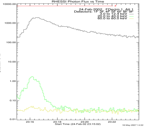
Figure 1: The light curves for flare 2 from Table 2, which has GOES class C2.7. Fluxes are in units of ph/$({\rm cm^{2}}\,{\rm s}\,\,{\rm keV}$).

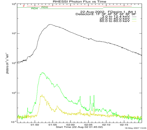
Figure 2: The light curves for flare 23 from Table 2, which has GOES class M5.6. Fluxes are in units of ph/$({\rm cm^{2}}\,{\rm s}\,\,{\rm keV}$).

3 Scaling laws for solar flares

Fig. 3 shows the correlation between the peak emission in the 1.6-12.4 keV band, as observed by GOES, and the RHESSI 20-40 keV band peak emission, for all flares in our sample (Table 2). The representative error bar on the RHESSI data has been estimated from the data itself combining the error on the peak flux and on the background. For the peak we considered the fluctuations around the peak in a short binning of 4 seconds. Typical values were 15$\%$ for the 20-40 keV band and 10$\%$ for the 60-80 keV band. For the background we took the peak to peak excursion and for the GOES band we estimated an error of 20$\%$.

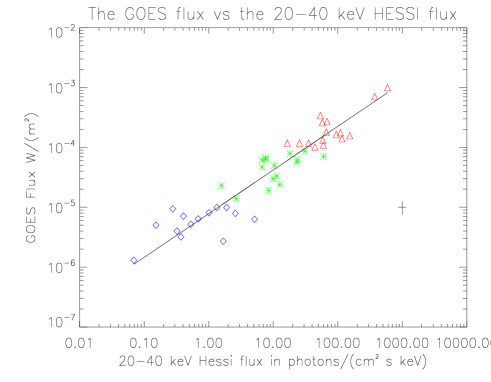
Figure 3: The peak emission in the 1.6-12.4 keV band from GOES data as a function of the peak emission in the 20-40 keV band, from RHESSI data, for all flaring events in our sample. Blue diamonds, green stars and red triangles correspond to C, M and X class respectively. A representative error bar is shown in the lower right part of the plot.

The two quantities are well correlated, and a scaling law in the form of a power law can be derived, applying the bisector regression method as described in Isobe et al. (1990):

$$F_{\rm G}\sim 7.83\times 10^{-6}\leavevmode\nobreak\ F_{(20-40)}^{0.73}$$ (1)

where $F_{\rm G}$ is the GOES peak flux 1.6-12.4 keV band in units of ${\rm Watt}/{\rm m}^{2}$ and $F_{20-40}$ is the peak flux in the 20-40 keV band, in ${\rm ph}/({\rm cm}^{2}\,{\rm s}\,\,{\rm keV})$. The slope for the power law is $0.73\pm 0.04$ and the intercept is $(7.83\pm 0.98)\times 10^{-6}$. This correlation holds over more than 3 orders of magnitude in GOES peak flux. An analysis on the comparison between this scaling law and the one found in Battaglia et al. (2005) is included in the Section 5.

In Fig. 4 we present the same type of analysis as in Fig. 3 but considering peak emission in the 60-80 keV band. Note that the number of events here is less than for the 20-40 keV band, as for the weaker flares no emission is detected in the 60-80 keV band. The flares for which a 60-80 keV peak flux has been determined are indicated with an asterisk in Table 2.

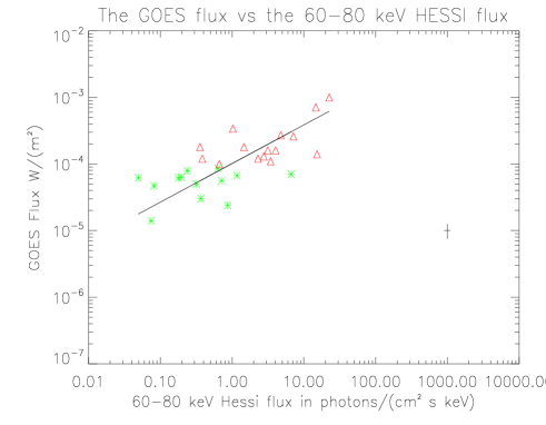
Figure 4: The peak emission in the 1.6-12.4 keV band from GOES data as a function of the peak emission in the 60-80 keV band, from RHESSI data, for all flare events with detectable 60-80 keV fluxes. Green stars and red triangles correspond to M and X class events respectively. A representative error bar is shown in the lower right part of the plot.

Although the spread is more significant than in the case of the 20-40 keV flux, a correlation between soft and hard peak fluxes is still well visible. We derived, using the same approach as for Eq. 1, a power law

$$F_{\rm G}\sim 1.02\times 10^{-4}\,\,F_{(60-80)}^{0.58}$$ (2)

where the units are the same in Eq. 1 and the slope is $0.58\pm 0.07$ and the intercept $(1.01\pm 0.13)\times 10^{-4}$.

3.1 Thermal contribution to the hard band flux

We have considered the total peak flux in each band, regardless of its origin. To determine which fraction of the observed flux is of thermal origin, we have developed a procedure to subtract from the total peak flux observed in the 20-40 and in the 60-80 bands the thermal component, as a function of the peak flare temperature, using a set of model spectra. This is necessary to compare the predictions of our scaling laws with the observations of intense stellar flares, where the observed plasma temperatures are much higher than for solar flares and thermal emission can be significant also in these bands.

To do this, we have simulated a set of thermal spectra and determined the relationship between the flux in the GOES 1.6-12.4 keV band and the flux in the 20-40 and 60-80 keV bands as a function of the peak temperature of the flare. We used the XSPEC package (Schwartz 1996; Smith et al. 2002) with a MEKAL thermal model, a plasma emission code which implements the optically-thin collisional ionization equilibrium emissivity model described in Mewe et al. (1995). For different temperatures we determined the value of the fluxes in the different bands of interest, 1.6-12.4, 20-40 keV and 60-80 keV. In Fig. 5 we plot the flux (as given by the model) in the 1.6-12.4 keV versus the flux in the 20-40 keV band for different temperatures ranging from 1 keV to 20 keV.

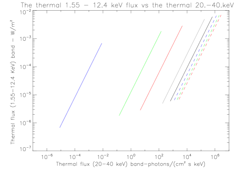
Figure 5: The flux in the 1.6-12.4 keV band as a function of the flux in the 20-40 keV band for a MEKAL thermal models, for temperatures of 1, 2, 3, 6, 9, 12, 16, and 20 keV from left to right, which correspond respectively to $\sim$12, 23, 35, 70, 104, 139, 186 and 232 $\times$ 10⁶K.

The relationship between the flux in the two bands is obviously linear, with a proportionality constant which depends on the temperature. Writing the relation as

$$F_{(20-40)}=m\cdot F_{\rm G}$$ (3)

and using the same units as before, i.e. $F_{\rm G}$ in ${\rm W}/{\rm m}^{2}$ and $F_{(20-40)}$ in ${\rm ph}/({\rm cm}^{2}\,{\rm s}\,\,{\rm keV})$, the values of $m$ for different temperatures are given in Table 3, for both the 20-40 and the 60-80 keV band.

Table 3: The values of $m$ in giving the proportionality between the thermal flux in the 20-40 and 60-80 keV bands ($F_{(20-40)}$ and $F_{(60-80)}$ and the thermal flux in the GOES 1.6-12.4 keV band ($F_{\rm G}$), with $F_{\rm G}$ in ${\rm W}/{\rm m}^{2}$ and $F_{(20-40)}$ and $F_{(60-80)}$ in ${\rm ph}/({\rm cm}^{2}\,{\rm s}\,\,{\rm keV})$.

Temp. (keV)	$m$, 20-40 keV	$m$, 60-80 keV
2	$7.93\times 10^{4}$	$4.10\times 10^{-5}$
3	$1.62\times 10^{6}$	0.69
6	$3.62\times 10^{7}$	$1.27\times 10^{4}$
9	$1.08\times 10^{8}$	$3.63\times 10^{5}$
12	$1.92\times 10^{8}$	$1.98\times 10^{6}$

While we cannot attribute a peak temperature individually to each flare in our sample, Feldman et al. (1995) found a tight correlation between peak flare intensity (up to GOES class X1) and peak temperature, allowing us to attribute an average temperature for some reference classes of flares. For each of these temperatures we calculate the thermal contribution with XSPEC and the corresponding total predicted flux obtained reversing the scaling law in Eq.1 which gives the following expression:

$$F_{(20-40)}\sim 9.908\times 10^{6}F_{\rm G}^{1.37}$$ (4)

in the same units used above.

We computed the ratio between the peak total flux (obtained from Eq. 4) and the average peak thermal flux in the 20-40 keV band. The results are shown in Table 4.

Table 4: The ratio between the peak thermal and non-thermal flux in the 20-40 keV band as a function of the flare GOES class. The first column reports the class of flares, the second column the average peak temperature as derived from Feldman et al. (1995), the third column the peak thermal flux (in units ${\rm ph}/{\rm cm}^{2}\,{\rm s}\,\,{\rm keV}$) from the MEKAL models, and the last column the ratio between the total peak flux derived by the scaling law in Eq. 4 and the average peak thermal flux.

Class	Average $T$ (keV)	$F_{\rm th(20-40)}$	$F_{(20-40)}/F_{\rm th(20-40)}$
C1	1.30	0.00058	$\sim$ 100
C4	1.47	0.02	$\sim$ 24
M1	1.64	0.10	$\sim$ 14
M4	1.70	0.54	$\sim$ 17
X1	2.00	7.92	$\sim$ 4

We can see that the thermal contribution to the peak flux in the 20-40 keV band is negligible in the less intense flares, and can be relevant in the 20-40 keV band only for the more intense events and and for temperatures close to the maximum that is observed on the Sun.

Using the data in Table 3 and Eq. 1 for a temperature of around 2 keV, for instance, we find that a value above $F_{G}\sim 3\times 10^{-6}\,\,{\rm W}/{\rm m}^{2}$ is required in order to have a total predicted $F_{(20-40)}$ emission higher or equal to the thermal component. This means that temperatures of the order of 20 $\times$ 10⁶K could be reached most likely for flares in M and X class, which is consistent with the result found by Feldman et al. (1995).

In Fig. 6 we show the same data as in Fig. 3 for the peak emission during our sample of solar flares, with superimposed the relation between the thermal flux in the GOES band versus the thermal flux in the 20-40 keV band for a peak temperature of 1.5, 2.0 and 3.0 keV, spanning the range of temperatures observed in solar flares from the C1 to the X10 classes. The class X flares are all located between the loci for the thermal fluxes for plasma at 2.0 and 3.0 keV (peak temperatures which are not exceptional for class X events). If the temperatures associated to our observed flares were lower than 2 keV, the fluxes would be totally dominated by non-thermal effects. For temperatures around 2.5 keV a part of the emission in this band, for the intense solar flares, should be given by the tail of the thermal spectrum.

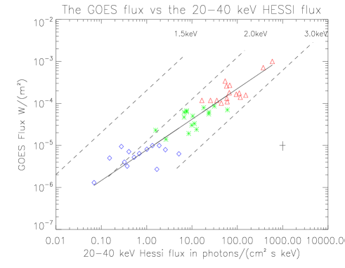
Figure 6: The same data as in Fig.3 with three additional dashed lines showing the thermal flux in the GOES band as a function of the thermal flux in the 20-40 keV band for peak flare temperatures of 1.5, 2.0 and 3.0 keV (spanning the range observed for solar flares from the C1 to the X10 class).

In Fig. 7 we show the same data as in Fig. 6 for the 60-80 keV band. In this band the observed emission is entirely non-thermal: to contribute to the observed flux the thermal plasma would need to have temperatures $\ga 6$ keV, that is much higher than what is observed in solar events.

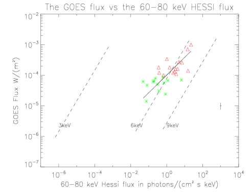
Figure 7: The same as Fig.4 with three additional dashed lines showing the thermal flux in the GOES band as a function of the thermal flux in the 60-80 keV band for plasma at 3.0, 6.0, 9.0 keV.

4 Stellar flares

In the previous section we have established a scaling law between the peak flare emission in the GOES, 20-40 keV and 40-60 keV bands in solar flares, including the strongest X-class. In this section we go further and determine whether the same law extends to the emission from intense stellar flares. This is a step beyond all previous studies which provides interesting new results.

For this purpose we have compared the extrapolation of the solar scaling law to the fluxes observed in stellar events with the few available broad-band data from intense stellar flares. The only observatory which has to date performed broad-band observations of stellar flares, from 0.1 up to $\simeq 100$ keV has been BeppoSAX (Boella et al. 1997a). We have analyzed the data from the MECS (1.6-10 keV) (Boella et al. 1997b) and PDS (15-300 keV) (Frontera et al. 1997) instruments for the flares observed on UX Ari, (Franciosini et al. 2001), Algol, (Favata et al. 2001) and AB Dor (2 events, Maggio et al. 2000). For the purpose of the present paper we needed to derive the peak fluxes in the 3 bands of interest, distinguishing the total, thermal and non-thermal fluxes.

We extrapolated the solar scaling laws, and used the peak flux in the GOES band (determined from our analysis of the BeppoSAX data) for each stellar flare to determine the predicted flux in the 20-40 and 60-80 keV band, using Eq. 4 and the following one:

$$F_{(60-80)}\sim 7.680\times 10^{6}\,F_{G}^{1.72}.$$ (5)

The results are shown in Fig. 8 for the 20-40 keV band and in Fig. 9 for the 60-80 keV band (where the stellar fluxes have been rescaled to a 1 AU distance, for ease of comparison). The horizontal error bars for the stellar events represent the uncertainties in the 20-40 keV flux resulting from the uncertainty in the slope of the best-fit correlation for the solar flares.

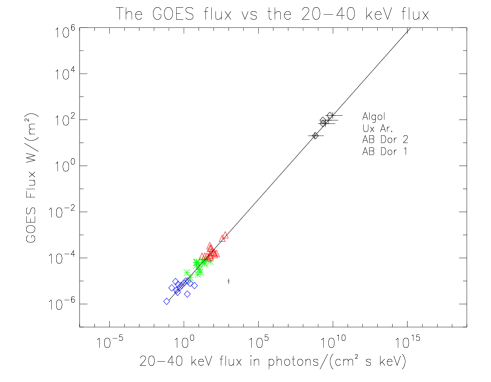
Figure 8: The scaling law for the peak emission during solar flares, extrapolated to the regime of intense stellar flares, showing the relation between the peak flux in the GOES band versus the peak flux in the 20-40 keV band. The solar correlation (Eq. 4) is shown, extrapolated to the peak GOES flux of stellar flares. The diamonds, stars and triangles represent the data from C, M and X class solar flares on the bottom left side. The black crosses show the corresponding location for the flares observed in the named stars in the top right side, using their peak flux in the GOES band, with the horizontal error bar representing the uncertainty induced by the uncertainty in the slope of the best fit correlation. The diamonds on the left side of the data point for each star show the relation between the non-thermal peak flux as derived from the BeppoSAX data.

Table 5 reports the results of this analysis for the 20-40 keV and 60-80 keV bands, respectively, giving, for each flare, the best-fit peak flux as deduced by the scaling law (Eq. 4 and Eq. 5, scaled to the respective distance of each star), with the uncertainty induced by the uncertainty in the best-fit scaling law. The best-fit for the total peak flux as measured on the BeppoSAX spectra is also reported.

We have performed a new analysis of the data, and we tried different possible models to fit the spectra. In particular we investigated if the presence of a non-thermal power law component could have produced a better fit, especially for the PDS instrument. The results obtained showed that the precision of the data at hand is not sufficient to draw any conclusion. A multi-temperature fit or a one-temperature plus a power-law fit are equally statistically acceptable. This means that we cannot exclude for sure the fact that this component has already been observed with BeppoSAX but not even demonstrate its presence. A recent study by Osten et. al. 2007 also investigates possible non-thermal emission in a stellar flare.

Table 5: For each of the 4 intense stellar flares observed by BeppoSAX, the peak flux in the 20-40 keV band and 60-80 keV as predicted by the extrapolation of the solar scaling law (column 2, Eq. 4 and Eq. 5) is given, together with its uncertainty (column 3). In column 4 the peak flux determined from the observations (using a fit including a power-law component) is given. Units are ${\rm ph}/{\rm cm}^{2}\,{\rm s}\,\,{\rm keV}$.

Event	$F_{(20-40)}$	Range	$F_{(20-40)}$
	scaling law		observed
Ux Ari	$0.47\times 10^{-4}$	$[0.15,2.12]\times 10^{-4}$	$0.20\times 10^{-4}$
Algol	$2.86\times 10^{-4}$	$[0.89,13.3]\times 10^{-4}$	$1.86\times 10^{-4}$
AB Dor, 1	$0.64\times 10^{-4}$	$[0.23,2.5]\times 10^{-4}$	$0.92\times 10^{-4}$
AB Dor, 2	$3.35\times 10^{-4}$	$[0.11,14.6]\times 10^{-4}$	$2.28\times 10^{-4}$
	$F_{(60-80)}$	Range	$F_{(60-80)}$
	scaling law		observed
UX Ari	$1.81\times 10^{-4}$	$[1.60\times 10^{-5},0.0053]$	$0.16\times 10^{-5}$
Algol	$1.29\times 10^{-3}$	$[1.06\times 10^{-4},0.043]$	$1.34\times 10^{-5}$
AB Dor, 1	$1.42\times 10^{-4}$	$[1.61\times 10^{-5},0.0039]$	$0.23\times 10^{-5}$
AB Dor, 2	$1.14\times 10^{-3}$	$[1.07\times 10^{-4},0.031]$	$2.42\times 10^{-5}$

From the upper part of Table 5 it is evident that the extension of the correlation observed for solar flares between the peak emission in the GOES band and the emission in the 20-40 keV band fits rather well the data for the intense stellar flares observed with BeppoSAX. In all cases, the observed peak flux in the 20-40 keV band is within the range of values predicted from the extension of the solar relationship. Given that this entails an extrapolation over the solar GOES band peak flux by four orders of magnitude, it is remarkable that the simple solar scaling law succeeds in predicting the 20-40 keV band flux also for stellar flares, also given that their peak plasma temperatures are much higher.

The lower part of Table 5 shows on the other hand that the extension of the solar correlation for the peak flux in the 60-80 keV band does not do a good job at predicting the peak flux in stellar events. In all cases, the predicted 60-80 keV peak flux is much higher than the observed value, by one to two orders of magnitude.

The correlation derived for the peak 60-80 keV flux in the solar case has a much steeper slope than the one derived for the peak 20-40 keV flux. In particular, when extrapolating toward very intense flares, the use of the solar correlations would predict that around class X100 000 (the most intense stellar flares are of class $\simeq$X1 000 000) the flux in the 60-80 keV band would exceed the one in the 20-40 keV band, leading to an “inverted spectrum” type of situation, contrarily to all available observational constraints.

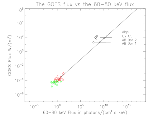
Figure 9: The same as Fig. 8 but for the 60-80 keV band.

The results in Table 5 are obtained considering a model with an additional power law, whereas in Table. 6 we give the values of the peak fluxes considering just the contribution from the thermal component.

From this table we can immediately deduce that in the 20-40 keV band almost all emission is of thermal origin while in the 60-80 keV, as for the Sun, it is the non thermal contribution which dominates.

Table 6: For each of the 4 intense stellar flares observed by BeppoSAX, the thermal contribution to the peak flux in the 20-40 keV band and 60-80 keV.Units are ${\rm ph}/{\rm cm}^{2}\,{\rm s}\,\,{\rm keV}$.

Event	$F_{(20-40)}^{th}$	$F_{(60-80)}^{th}$
Ux Ari	$0.24\times 10^{-4}$	$0.64\times 10^{-7}$
Algol	$1.2\times 10^{-4}$	$9.6\times 10^{-7}$
AB Dor, 1	$0.35\times 10^{-4}$	$0.43\times 10^{-7}$
AB Dor, 2	$1.4\times 10^{-4}$	$4.60\times 10^{-7}$

As the extrapolation to the intense stellar flares in this band of energy seems to not be in agreement with the data at hand, probably different mechanisms play a dominant role that becomes more evident for the very intense flares at the highest energies and that can justify the discrepancy in the extrapolation of the solar scaling law to stellar flares in the 60-80 keV band.

Beyond the “standard paradigm” for solar flares, which we have identified with the thick-target model of Brown (1971), other possibilities exist. In particular coronal hard X-ray sources of the type observed by Frost and Dennis (1971) and Hudson (1978) now seem to be almost routinely observed in major events by RHESSI (Krucker et al., 2007).

5 Discussion

The correlation law in solar flares represented by our Eq. 1 can be compared to the result found in Battaglia et al. 2005. They studied a sample of RHESSI flares, by performing spectral fits to separate the thermal emission from the non-thermal one (modeled as a power law), and restricting themselves to flares up to GOES class M5.9 (no X-class events were considered). They correlate the flux in the GOES band with the non-thermal monochromatic flux at 35 keV, find the scaling law

$$F_{\rm G}=1.8\times 10^{-5}F_{35}^{0.83}$$ (6)

where $F_{\rm G}$ is the flux in the GOES band and $F_{35}$ is the non-thermal flux at 35 keV as obtained through individual spectral fits, in the same units as in Eq. 1.

Considering the different approach adopted here, the two scaling laws are quite consistent, especially regarding the slope, in agreement with the expectation that the emission in the GOES band will be dominated by thermal emission for the complete range of temperatures spanned by solar flares, while at 35 keV the emission observed will be mostly of non-thermal origin.

On the other hand caution should be used in comparing directly Eq. 1 and Eq. 6 where different physical quantities appear. We used integrated fluxes in the 20-40 keV and 60-80 keV bands over all the energy, whereas Battaglia et al. used a monochromatic spectrum at 35 keV. This may justify a steeper slope in Eq. 6 than the one derived by us in Eq. 1.

We would like to stress the fact that we do not make spectral fits, which is also a major difference with the work by Battaglia. We decided to proceed in a non-parametric way because of the difficulty to estimate the low-energy cut-off of the power law from the data. This can produce a significant uncertainty in the determination of the thermal component. Data itself cannot constraint well the two components and then the derived parameters could be very uncertain.

In Fig. 10 we represent the same as in Fig. 9 with an additional fit obtained combining the solar data and the stellar observations.

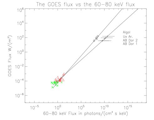
Figure 10: The same as in Fig. 9 with an additional fit obtained combining the solar RHESSI data and stellar flares observations.

This produces a scaling law

$$F_{(60-80)}\sim 6.20\times 10^{5}F_{\rm G}^{1.37}$$ (7)

which coincidentally has the same slope as in Eq. 4 for the 20-40 band. We remind that the scaling law for the 60-80 keV band has been deduced from a limited number of flares in Table 2 as the less intense events have a negligible emission at these high energies.

If future additional points would confirm the relation in Eq. 7, this would imply an universal slope across more than six orders of magnitude in flare strength, which will be a quite remarkable result.

6 Conclusions

We have studied the correlation between the peak flux emitted in three different energy bands (1.6-12.4 keV, or “GOES” band, 20-40 keV and 60-80 keV) for a number of solar flares spanning a broad range of peak flux in the GOES band (or “GOES class”). In the solar case, the GOES-band flux is almost completely dominated by the thermal emission of the flaring plasma, while the 60-80 keV flux is entirely due to non-thermal emission. This is likely due to the accelerated electrons which in the thick-target model of flares cause the evaporation of the plasma which is responsible for the thermal emission. The 20-40 keV emission contains contributions from both the tail of the thermal spectrum and the non-thermal, power law spectrum, with the former increasing with the GOES class, which in solar flares is well correlated with the peak temperature of the flare.

The analyzed sample of solar flares spans 3 orders of magnitude in GOES class (from C1 to X10), and both the 20-40 keV and the 60-80 keV peak flux are well correlated with the GOES band peak flux. The good correlation for the 60-80 keV band (which in the solar case is purely non-thermal in origin) may be construed to imply support for a “thick-target” type of framework, in which the thermal emission is linked to the non-thermal one by a causal relationship.

We have then studied the applicability of these scaling laws to the case of intense stellar flares. Our sample is small, limited by the availability of the data: BeppoSAX has been the only X-ray observatory with the broad-band response needed for these observations, and only 4 events have been detected in the hard bands. In the future, additional stellar flares may be observed with Suzaku, and, later with the proposed Simbol-X hard X-ray telescope.

The extrapolation of the scaling laws derived for solar flares to the case of intense stellar flares (an extrapolation of 5 orders of magnitude in GOES peak flux) results in a quite remarkable good agreement between the predicted and observed 20-40 keV flux, while it over-predicts by some two orders of magnitude the 60-80 keV flux.

Future observations, increasing the statistic of intense flares, should allow to clarify the origin of this discrepancy. If a power law like the one in Eq. 7 is found, the extrapolation would be possible for both bands and the two scaling laws would be defined by the same slope, which would be an even more remarkable result.

- (1) Antonucci E., et al. 1982, Solar Phys., 78, 107.
- (2) Antonucci E., Gabriel A. H., Dennis B. R., 1984, ApJ 287, 917
- (3) Battaglia, M., Grigis, P. C. Benz, A. O. 2005, AA, 439, 737
- (4) Boella G., Butler R.C., Perola G.C. et al., 1997a, AA 122, 299
- (5) Boella G., Chiappetti L., Conti G. et al., 1997b, AA 122, 341
- (6) Brown, J. C. 1971, Sol. Phys., 18, 489
- (7) Brown, J. C. 1973, Sol. Phys., 31, 143
- (8) Favata, F. and Schmitt, J. H. M. M., AA, 350, 900-916
- (9) Favata, F. et al., arXiv:astro-ph/0506134, Accepted to ApJS.
- (10) Feldman, U., Laming, J. M and Doscher, G. A., 1995, ApJ, 451, L79-l81
- (11) Fisher, G. H., Canfield, R. C., McClymont, A. N. 1985a,Apj, 289, 414;mFisher, G. H., Canfield, R. C., McClymont, A. N. 1985b,Apj, 289, 425;
- (12) Fletcher, L. Hudson, H. S. 2002, Sol. Phys., 210, 307
- (13) Franciosini, E. , Pallavicini, R. and Tagliaferri, G., AA. 375, 196-204
- (14) Frontera F., Costa E., Dal Fiume D. et al., 1997, AA 122, 371
- (15) Frost, K. J., and Dennis, B. R. 1971, ApJ, 165, 655
- (16) Garcia, H. A. 1994, Sol. Phys., 154, 275
- (17) Grigis, P and Benz, A, AA 434, 1173-1181,2005.
- (18) Güdel, M., Benz, A. O., Schmitt, J. H. M. M., Skinner, S. L. 1996, ApJ, 471, 1002
- (19) Hawley, S. L., Fisher, G. H., Simon, T., et al. 1995, ApJ, 453, 464
- (20) Hudson, H. S. 1972, Sol. Phys., 24, 414
- (21) Hudson, H. S. 1978, ApJ, 224, 235
- (22) Hudson, H. S. Fárník, F. 2002, in ESA SP-506: Solar Variability : From Core to Outer Frontiers, 261-264
- (23) Krucker, S. et al. 2007, in preparation
- (24) Isobe, T., Feigelson, E. D., Akritas, M. G., Babu, G. J. 1990, Apj, 364, 104
- (25) Lin, R. P., Hudson, H. S. 1971, Sol. Phys., 17, 412
- (26) Lin, R. P., Hudson, H. S. 1976, Sol. Phys., 50, 153
- (27) Lin, R. P. et al. 2002, Sol. Phys., 210, 3
- (28) Maggio, A. , Pallavicini, R. , Reale, F. and Tagliaferri, G. , 2000, AA, 356, 627
- (29) Matsumoto, Y. et al,Vol.57, No.1, pp. 211-220
- (30) Mewe R., Kaastra J.S., Liedahl D.A., 1995, Legacy 6, 16
- (31) Neupert, W. M. 1968, Apj, 153, L59
- (32) R. A. Osten, S. Drake, J. Tueller, J. Cummings, M. Perri, A. Moretti, S. Covino, 2006, astro-ph/0609205, accepted for publication in Astrophysical Journal.
- (33) Parks, G. K. and Winckler, J. R., 1969, ApJ, 155, L117
- (34) Petrosian, V. 1973, ApJ, 186, L59
- (35) Schwartz, R. A. 1996, Compton Gamma Ray Observatory Phase 4 Guest Investigator Program: Solar Flare Hard X-ray Spectroscopy, Technical Report, NASA Goddard Space Flight Center
- (36) Schwartz, R. A., Csillaghy, A., Tolbert, A. K., Hurford, G. J., Mc Tiernan, J. and Zarro, D. 2002, Sol. Phys., 210, 165
- (37) Saint-Hilaire, P., Von Praun, C., Stolte, E., et al. 2002, Sol. Phys., 210, 143
- (38) Schnopper, H. W., Thompson, R. J., and Watt, S. 2002, Space Sci. Rev., 8, 534
- (39) Smith, D. M. et al. 2002, Sol. Phys., 210, 33
- (40) Veronig, A., Vrsnak, B., Dennis,B.R., Temmer, M., Hanslmeier, A., Magdalenic, J., astro-ph/0208089, “Magnetic Coupling of the Solar Atmosphere”, Proceedings of the Euroconference and IAU Colloquium 188, Santorini, Greece, June 2002, ed. H. Sawaya-Lacoste, ESA SP-505.