Causality and Micro-Causality in Curved Spacetime

Abstract:

We consider how causality and micro-causality are realised in QED in curved spacetime. The photon propagator is found to exhibit novel non-analytic behaviour due to vacuum polarization, which invalidates the Kramers-Kronig dispersion relation and calls into question the validity of micro-causality in curved spacetime. This non-analyticity is ultimately related to the generic focusing nature of congruences of geodesics in curved spacetime, as implied by the null energy condition, and the existence of conjugate points. These results arise from a calculation of the complete non-perturbative frequency dependence of the vacuum polarization tensor in QED, using novel world-line path integral methods together with the Penrose plane-wave limit of spacetime in the neighbourhood of a null geodesic. The refractive index of curved spacetime is shown to exhibit superluminal phase velocities, dispersion, absorption (due to $\gamma\to e^{+}e^{-}$) and bi-refringence, but we demonstrate that the wavefront velocity (the high-frequency limit of the phase velocity) is indeed $c$, thereby guaranteeing that causality itself is respected.

1 Introduction

The purpose of this letter is to consider how causality and micro-causality are realised in quantum field theory in curved spacetime in the light of the discovery of novel non-analytic behaviour in the photon propagator due to vacuum polarization in QED [2].

These questions have arisen through the resolution of a long-standing puzzle in “quantum gravitational optics” [3, 4], viz. how to reconcile the fact that the low-frequency phase velocity $v_{\rm ph}(0)$ for photons propagating in curved spacetime may be superluminal [5] with the requirement of causality that the wavefront velocity $v_{\rm wf}=v_{\rm ph}(\infty)$ should not exceed $c$.

The reason why this is a problem is related to the Kramers-Kronig dispersion relation [9, 10]. In terms of the refractive index $n(\omega)$, where $v_{\rm ph}(\omega)=1/\text{Re}~{}n(\omega)$ (setting $c=1$), this is

$$\text{Re}\,n(\infty)-\text{Re}\,n(0)=-\frac{2}{\pi}\int_{0}^{\infty}\frac{d\omega}{\omega}\,\text{Im}\,n(\omega)\ .$$ (1)

Provided $\text{Im}~{}n(\omega)>0$, as required by unitarity in the form of the optical theorem, this implies $\text{Re}\,n(\infty)<\text{Re}\,n(0)$ and hence $v_{\rm ph}(\infty)>v_{\rm ph}(0)$. The fundamental assumption in the derivation of eq. (1) is that $n(\omega)$ is analytic in the upper-half complex $\omega$ plane, which is generally presented (see, e.g. ref. [11]) in flat spacetime as a direct consequence of micro-causality.

The resolution of this apparent paradox is that the Kramers-Kronig dispersion relation does not hold in the form (1). We find that $n(\omega)$ develops branch-point singularities on the imaginary axis in the upper-half plane. The consequent modification of eq. (1) then allows $\text{Re}\,n(\infty)>\text{Re}\,n(0)$ and we find by explicit calculation of the full non-perturbative frequency dependence of the refractive index that $n(\infty)$ is indeed equal to 1 and the wavefront velocity itself is $v_{\rm wf}=c$. Remarkably, we find that these unusual analyticity properties can be traced very directly to the focusing property of null congruences and the existence of conjugate points, which are, in turn, a consequence of the null energy condition. Conjugate points are points in spacetime that are joined by a family of geodesics: at least in an infinitesimal sense, see fig. (1). Such infinitesimal deformations are associated to zero modes that lead directly to the branch points on the imaginary axis.

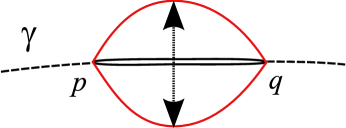
Figure 1: Points $p$ and $q$ on a geodesic $\gamma$ are conjugate if they can be joined—at least in an infinitesimal sense—by a family of geodesics close to $\gamma$. The existence of conjugate points means that the classical saddle-point solution with the photon connected at $p$ and $q$ to a degenerate $e^{+}e^{-}$ loop squashed onto the geodesic $\gamma$ is deformable into a non-degenerate loop as shown.

The refractive index in QED is determined by the vacuum polarization tensor $\Pi_{\mu\nu}(k)$. On-shell, and in a basis diagonal with respect to the polarizations $\hat{\varepsilon}_{i}$ ($i=1,2$), the relation is

$$n_{i}(\omega)=1+{1\over\omega^{2}}\Pi_{ii}(\omega)\ .$$ (2)

We have, for the first time, evaluated the complete non-perturbative frequency dependence of the vacuum polarization $\Pi_{ij}(\omega)$ in QED in curved spacetime by combining two powerful techniques:  (i) the world-line sigma model, which enables the non-perturbative frequency dependence of $\Pi_{ij}(\omega)$ to be calculated using a saddle-point expansion about a geometrically motivated classical solution and  (ii) the Penrose plane-wave limit, which encodes the relevant tidal effects of the spacetime curvature in the neighbourhood of the original null geodesic traced by the photon in the classical theory.

2 The World-Line Sigma Model, Penrose Limit and Null Congruences

In the world-line formalism for scalar QED, the one-loop vacuum polarization tensor is given by

$$\Pi^{\text{1-loop}}_{ij}=\frac{\alpha}{4\pi}\int_{0}^{\infty}\frac{dT}{T^{3}}\int_{0}^{T}d\tau_{1}\,d\tau_{2}\,{\cal Z}\,\big{\langle}V^{*}_{\omega,\varepsilon_{i}}[x(\tau_{1})]V_{\omega,\varepsilon_{j}}[x(\tau_{2})]\big{\rangle}\ .$$ (3)

Here, $V_{\omega,\varepsilon_{i}}[x(\tau)]$ are vertex operators for the photon and the expectation value is calculated in the 1-dim world-line sigma model involving periodic fields $x^{\mu}(\tau)=x^{\mu}(\tau+T)$ with an action

$$S=\int_{0}^{T}d\tau\,\Big{(}\frac{1}{4}g_{\mu\nu}(x)\dot{x}^{\mu}\dot{x}^{\nu}-m^{2}\Big{)}\ ,$$ (4)

where $g_{\mu\nu}$ is the metric of the background spacetime. The expectation value is represented to ${\cal O}(\alpha)$ by an $e^{+}e^{-}$ loop with insertions of the photon vertex operators at $\tau_{1}$ and $\tau_{2}$, as illustrated in fig. (2). The factor ${\cal Z}$ is the partition function of the world-line sigma model relative to flat space.

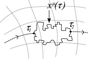
Figure 2: The $e^{+}e^{-}$ loop $x^{\mu}(\tau)$ with insertions of photon vertex operators at $\tau_{1}$ and $\tau_{2}$.

The form of the vertex operators is determined at this order by the classical equations of motion for the gauge field $A_{\mu}(x)$ in the geometric optics, or WKB, limit. That is,

$$V_{\omega,\varepsilon_{i}}[x]=\dot{x}^{\mu}A_{\mu}(x)$$ (5)

where

$$A_{\mu}(x)={\cal A}(x)\hat{\varepsilon}_{i\mu}(x)e^{i\omega\Theta(x)}+\cdots\ ,$$ (6)

where ${\cal A}$ is the scalar amplitude, $\hat{\varepsilon}_{i}$ are the polarizations and the phase $\Theta$ satisfies the eikonal equation

$$g^{\mu\nu}\partial_{\mu}\Theta\partial_{\nu}\Theta=0\ .$$ (7)

The solution determines a congruence of null geodesics where $\ell^{\mu}=\partial^{\mu}\Theta$ is the tangent vector to the null geodesic in the congruence passing through the point $x$. In the particle interpretation, $k^{\mu}=\omega\ell^{\mu}$ is momentum of a photon travelling along the geodesic. The polarization vectors $\hat{\varepsilon}_{i}^{\mu}$ are orthogonal to $\ell^{\mu}$ and are parallel transported: $\ell\cdot D\,\hat{\varepsilon}_{i}^{\mu}=0$, while the scalar amplitude satisfies

$$\ell\cdot D\,\log{\cal A}=-{1\over 2}D^{\mu}\ell_{\mu}\equiv-\hat{\theta}$$ (8)

where the expansion $\hat{\theta}$ is one of the optical scalars appearing in the Raychoudhuri equations.

In order to evaluate the world-line path integral over $x^{\mu}(\tau)$, we will need to consider fluctuations about the classical geodesic $\gamma$. The first step is to set up Fermi normal coordinates $(u,v,y^{i})$ [20] which are adapted to the null geodesic in the sense that $\gamma$ is the curve $(u,0,0,0)$ where $u$ is the affine parameter, $v$ is another null coordinate and $y^{i}$ parameterize the transverse subspace. Now, as explained in Section 3, the relevant curvature degrees of freedom needed to describe these fluctuations at leading order in an expansion in $R/m^{2}$ are captured in the Penrose limit of the spacetime around $\gamma$ [21, 22]. This follows from an overall Weyl re-scaling $ds^{2}\to\lambda^{2}ds^{2}$ of the metric obtained by an asymmetric re-scaling of the coordinates, $(u,v,y^{i})\to(u,\lambda^{2}v,\lambda y^{i})$, chosen so that the affine parameter $u$ is invariant. This leads, for an arbitrary background spacetime, to the plane wave metric

$$ds^{2}=2du\,dv+h_{ij}(u)y^{i}\,y^{j}\,du^{2}-dy^{i2}\ ,$$ (9)

where $h_{ij}(u)$ is related to the curvature of the original metric $g_{\mu\nu}$ by $h_{ij}=-R_{uiuj}$. This is the Penrose limit of the background spacetime in the neighbourhood of $\gamma$ in Brinkmann coordinates.

(a)   (b)

Figure 3: The behaviour of the congruence of null geodesics for the (a) Type I and (b) Type II plane wave metrics.

It is now convenient to divide these spacetimes into two classes, depending on the behaviour of the null congruence. Introducing a second optical scalar, the shear $\hat{\sigma}=\sqrt{\tfrac{1}{2}D_{(\mu}\ell_{\nu)}D^{\mu}\ell^{\nu}-\hat{\theta}^{2}}$, we can write the Raychoudhuri equations in the form:

$$\begin{split}\partial_{u}({\hat{\theta}}+{\hat{\sigma}})&=-(\hat{\theta}+\hat{\sigma})^{2}-\Phi_{00}-|\Psi_{0}|\ ,\\ \partial_{u}({\hat{\theta}}-{\hat{\sigma}})&=-(\hat{\theta}-\hat{\sigma})^{2}-\Phi_{00}+|\Psi_{0}|\ .\end{split}$$ (10)

Here, we have introduced the Newman-Penrose notation for the components of the Ricci and Weyl tensors: $\Phi_{00}={1\over 2}R_{uu}$ and $|\Psi_{0}|={1\over 2}(C_{u1u1}-C_{u2u2})$. The effect of expansion and shear is visualized by the effect on a circular cross-section of the null congruence as the affine parameter $u$ is varied: the expansion $\hat{\theta}$ gives a uniform expansion whereas the shear $\hat{\sigma}$ produces a squashing with expansion along one transverse axis and compression along the other. The combinations $\hat{\theta}\pm\hat{\sigma}$ therefore describe the focusing or defocusing of the null rays in the two orthogonal transverse axes. Provided the signs of $\Phi_{00}\pm|\Psi_{0}|$ remain fixed (as in the symmetric plane wave example considered in detail later) we can therefore divide the plane wave metrics into two classes (see fig. (3)). A Type I spacetime, where $\Phi_{00}\pm|\Psi_{0}|$ are both positive, has focusing in both directions, whereas Type II, where $\Phi_{00}\pm|\Psi_{0}|$ have opposite signs, has one focusing and one defocusing direction. Note, however, that there is no spacetime with both directions simultaneously defocusing, since the null-energy condition requires $\Phi_{00}\geq 0$.

It is clear that provided the geodesics are complete, those in a focusing direction will eventually cross. In fact, the existence of conjugate points, as described earlier, is generic in spacetimes satisfying the null energy condition [6, 23]. The existence of conjugate points plays a crucial rôle in the world-line path integral formalism since, as explained below, they imply the existence of zero modes in the partition function which ultimately are responsible for the Kramers-Kronig violating singularities in the vacuum polarization tensor.

First, we need the explicit solutions for the geodesic equations in the plane wave metric (9). With $u$ itself as the affine parameter, these are:

$$\partial_{u}^{2}v+2h_{ij}y^{i}\partial_{u}y^{j}+{1\over 2}\partial_{u}h_{ij}y^{i}y^{j}=0\ ,\qquad\partial_{u}^{2}y^{i}+h_{ij}y^{j}=0\ ,$$ (11)

the latter being the Jacobi equation for the geodesic deviation vector $y^{i}$. The solution for $v$ determines the eikonal phase [2]

$$\Theta(x)=v-{1\over 2}\Omega_{ij}y^{i}y^{j}\ ,$$ (12)

where $\Omega_{ij}=\partial_{u}E_{ia}E^{a}{}_{j}$ is most simply expressed in terms of a zweibein $E^{a}{}_{i}(u)$ in terms of which the curvature is $h_{ij}=-\partial_{u}^{2}E_{ia}E^{a}{}_{j}$. The polarization 1-forms and scalar amplitude are

$$\hat{\varepsilon}_{i}=dy^{i}-\Omega_{ij}y^{j}du\ ,\qquad{\cal A}=\sqrt{1\over{\rm det}E^{i}{}_{a}}\ .$$ (13)

These give all the ingredients necessary for the vertex operators, so we determine

$$V_{\omega,\varepsilon_{i}}[x^{\mu}(\tau)]=\big{(}\dot{y}^{i}-\Omega_{ij}y^{j}\dot{u}\big{)}~{}\sqrt{1\over{\rm det}E^{i}{}_{a}}~{}\exp i\omega\Big{[}v-{1\over 2}\Omega_{ij}y^{i}y^{j}\Big{]}\ .$$ (14)

3 World-line Calculation of the Vacuum Polarization

We have now assembled all the elements needed to calculate the world-line path integral (3) for the vacuum polarization. The fundamental idea is to evaluate this by considering the Gaussian fluctuations about a saddle point given by the classical solution of the equations of motion for the action

$$S=-T+\frac{m^{2}}{4T}\int_{0}^{1}d\tau\,g_{\mu\nu}(x)\dot{x}^{\mu}\dot{x}^{\nu}-\omega\Theta[x(\xi)]+\omega\Theta[x(0)]\ ,$$ (15)

including the phase $\Theta(x)$ of the vertex operators which act as sources. In (15), we have re-scaled $T\to T/m^{2}$, which makes it clear that $1/m^{2}$ plays the rôle of a conventional coupling constant. In fact, the effective dimensionless coupling is actually the dimensionless ratio $R/m^{2}$. (We have also re-scaled $\tau\to T\tau$ so that the $\tau$ integral now runs from 0 to 1.)

The sources act as impulses which insert world-line momentum at the special points $x(0)$ and $x(\xi)$. In between these points, the classical solution is simply a null geodesic path and it is straightforward to see that this is given by $v=y^{i}=0$ while $u$ satisfies

$$\ddot{u}=-\frac{2\omega T}{m^{2}}\delta(\tau-\xi)+\frac{2\omega T}{m^{2}}\delta(\tau)\ .$$ (16)

The solution is [2]

$$u=\tilde{u}(\tau)=-u_{0}+\begin{cases}2\omega T(1-\xi)\tau/m^{2}&0\leq\tau\leq\xi\ ,\\ 2\omega T\xi(1-\tau)/m^{2}&\xi\leq\tau\leq 1\ ,\end{cases}$$ (17)

where $u_{0}=\omega T\xi(1-\xi)/m^{2}$. This describes an $e^{+}e^{-}$ loop squashed down to lie along the original photon null geodesic between $u=\pm u_{0}$ as illustrated in fig. (1).

An intriguing aspect of this is that the affine parameter length of the loop actually increases as the frequency $\omega$ is increased. Technically, this is simply because for higher frequencies the sources impart larger impulses. However, it means that in the high frequency limit, the photon vacuum polarization probes the entire length of the null geodesic and becomes sensitive to global aspects of the null congruence. This is rather counter-intuitive, since we would naively expect high frequencies to probe only local regions of spacetime, and appears to be yet another example of the sort of UV-IR mixing phenomenon seen in other contexts involving quantum gravity or string theory.

Another crucial point is that while (17) is the only general solution, for specific values of $T$ (or equivalently $\omega$) there are further solutions. These are due to the existence of conjugate points on the null geodesic. For values of $T$ for which $v(\pm u_{0})=y^{i}(\pm u_{0})=0$, there exists more than one null geodesic path between the points $\tau=0,\xi$ where the impulses are applied. This gives rise to a continuous set of classical solutions, which results in zero modes in the path integral for these specific values of $T$: see fig. (1). In turn, these produce the singularities in the partition function which are responsible for the violation of the Kramers-Kronig relation. Notice, that it is not necessary that these more general geodesics lift from the Penrose limit to the full metric.

The perturbative expansion in $R/m^{2}$ about this solution can be made manifest by an appropriate re-scaling of the “fields” $x^{\mu}(\tau)$. However, this re-scaling must be done in such a way as to leave the classical solution $\tilde{u}(\tau)$ invariant. But this is precisely (see ref.[2] for details) the Penrose re-scaling described above, where $\lambda$ is identified with the effective coupling $R/m^{2}$. This is why the physics of vacuum polarization is captured perturbatively in ${\cal O}(R/m^{2})$ by the Penrose expansion in ${\cal O}(\lambda)$ [20, 2] of the background spacetime around the photon’s null geodesic $\gamma$.

Expanding around the classical solution, in the plane wave metric (9), we find the Gaussian fluctuations in the transverse directions (the $u$, $v$ fluctuations are identical to flat space) are governed by the action

$$S^{(2)}=\int_{0}^{1}d\tau\,\Big{[}-\frac{1}{4}\big{(}\dot{y}^{i2}+\dot{\tilde{u}}^{2}h_{ij}(\tilde{u})y^{i}y^{j}\big{)}+\frac{\omega T}{2m^{2}}\Omega_{ij}(\tilde{u})y^{i}y^{j}\big{(}\delta(\tau-\xi)-\delta(\tau)\big{)}\Big{]}\ .$$ (18)

At this point, in order to illustrate the general features of our analysis with a simple example, we restrict the plane wave background to the special case where the curvature tensor is covariantly constant. This defines a locally symmetric spacetime, and the corresponding “symmetric plane wave” has metric (9) with

$$h_{ij}y^{i}y^{j}=\sigma_{1}^{2}(y^{1})^{2}+\sigma_{2}^{2}(y^{2})^{2}\ .$$ (19)

The curvatures are $R_{uu}=\sigma_{1}^{2}+\sigma_{2}^{2}$ and $C_{u1u1}=-C_{u2u2}={1\over 2}(\sigma_{2}^{2}-\sigma_{1}^{2})$. The signs of the coefficients determine which class the spacetime belongs to. For Type I (focus/focus), $\sigma_{1}$ and $\sigma_{2}$ are both real, while Type II (focus/defocus) has $\sigma_{1}$ real and $\sigma_{2}$ imaginary. The case $\sigma_{1},\sigma_{2}$ both imaginary is forbidden by the null energy condition, which requires $R_{uu}>0$. With this background, the geodesic equations determine the zweibein $E^{i}{}_{a}{}=\delta_{ai}\cos(\sigma_{i}u+a_{i})$ and $\Omega_{ij}=-\delta_{ij}\sigma_{i}\tan(\sigma_{i}u+a_{i})$ (the $a_{i}$ are arbitrary integration constants).

The core of the calculation reported in ref.[2] is the evaluation of the partition function ${\cal Z}$ and the two-point function $\langle\hat{\varepsilon}_{i}\cdot\dot{x}~{}\hat{\varepsilon}_{j}\cdot\dot{x}\rangle$ for the world-line path integral (3) in the symmetric plane wave background. A lengthy calculation described in detail in [2] eventually gives the following result for the vacuum polarization:

$$\Pi^{\text{1-loop}}_{ij}=-\delta_{ij}\frac{\alpha m^{2}}{2\pi}\int_{0}^{\infty+i\epsilon}\frac{dT}{T^{2}}e^{-T}\int_{0}^{1}d\xi\,\left\{1-\frac{\beta_{i}}{\sinh\beta_{i}\cosh\beta_{i}}\prod_{l=1}^{2}\sqrt{\frac{\beta_{l}^{3}}{\sinh^{3}\beta_{l}\cosh\beta_{l}}}\right\}\ .$$ (20)

where $\beta_{i}=\omega T\xi(1-\xi)\sigma_{i}/m^{2}$. In deriving (20), we have performed a Wick rotation $T\to-iT$ to leave a convergent integral. The $i\epsilon$ prescription deals with the singularities on the real axis which arise in the Type II case.

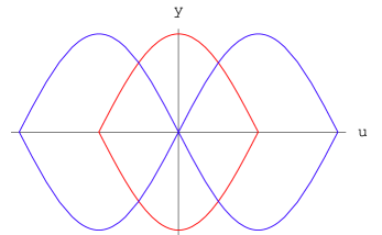
Figure 4: The $n=1$ (red) and $n=2$ (blue) zero modes for $\xi=\tfrac{1}{2}$. The points $u=\pm u_{0}$ are conjugate points for $\gamma$.

This expansion demonstrates clearly the unconventional analyticity properties of the vacuum polarization in curved spacetime. When $\sigma_{i}$ is real, there are branch point singularities on the imaginary $T$ axis at the specific values

$$T=\frac{i\pi m^{2}n}{2\xi(1-\xi)\sigma_{i}\omega}\ ,\qquad n=1,2,\ldots\ .$$ (21)

These singularities arise from zeros of the fluctuation determinant ${\cal Z}$ and have a natural interpretation in terms of zero modes, i.e. non-trivial solutions of the fluctuation equations that follow by varying (18) with respect to $y^{i}$. For the special case $\xi=\tfrac{1}{2}$, these zero modes are particularly simple to write down: $u=\tilde{u}(\tau)$ as in (17) while

$$y^{i}(\tau)=\sin(2n\pi\tau)\ .$$ (22)

The $n=1$ and $n=2$ zero modes are illustrated in fig. (4). (For generic $\xi$, the zero modes are more complicated: see ref.[2].) This confirms that the zero modes are associated to geodesics that intersect $\gamma$ at both $u=\pm u_{0}$, i.e. the conjugate points on the geodesic $\gamma$. In terms of the vacuum polarization $\Pi_{ij}^{\text{1-loop}}(\omega)$ or the refractive index $n_{i}(\omega)$, these singularities appear on the imaginary axis in the upper-half plane in $\omega$. They have profound consequences for the Kramers-Kronig dispersion relation.

In the Type II case, where one of the $\sigma_{i}$ is imaginary, there are also singularities on the real $T$ axis. These singularities can also be understood in terms of zero modes, but now with imaginary affine parameter $u\to iu$, and can be thought of as world-line instantons. These give rise to an imaginary part for $\Pi_{ij}^{\text{1-loop}}(\omega)$ and the refractive index $n(\omega)$, which corresponds to the tunnelling process $\gamma\to e^{+}e^{-}$ in the background gravitational field.

4 Refractive Index in Curved Spacetime

The refractive index follows immediately from the result (20) for the vacuum polarization. We present the results for the Type I and Type II symmetric plane wave backgrounds separately.

Type I:   This includes the special case of conformally flat spacetimes, where $\sigma_{1}=\sigma_{2}\equiv\sqrt{R}$. Evaluating (20) numerically gives the result shown in fig. (5). Here, both polarizations are superluminal at low frequencies, with the refractive index rising monotonically to the high-frequency limit $n(\omega)\to 1$. The wavefront velocity, $v_{\rm wf}=v_{\rm ph}(\infty)$ is therefore $c$, in accordance with our expectations from causality. The integrand in (20) is regular on the real axis and so $\text{Im}~{}n(\omega)$ is vanishing and there is no pair creation.

We can find explicit analytic expressions for $n(\omega)$ in these limits [2]. For low frequencies,

$$n_{i}(\omega)=1-\frac{\alpha R}{2\pi m^{2}}\Big{[}\frac{1}{18}-\frac{71}{14175}\frac{\omega^{2}R}{m^{4}}+\frac{428}{189189}\Big{(}\frac{\omega^{2}R}{m^{4}}\Big{)}^{2}-\cdots\Big{]}\ .$$ (23)

This series is divergent but alternating and this is correlated with the fact that it is Borel summable, with the sum being defined by the convergent integral in (20) which has no singularities on the real axis. In the high-frequency limit, we find that the refractive index approaches 1 from below, with a $1/\omega$ dependence:

$$n_{i}(\omega)=1-\frac{\alpha C_{i}}{12\pi\omega}+{\cal O}\Big{(}\frac{\log\omega}{\omega^{2}}\Big{)}\,$$ (24)

where $C_{i}=\big{(}\frac{1}{3}+\frac{7\pi^{2}}{36}\big{)}\sqrt{R}$ for both $i=1,2$.

(a)   (b)

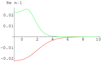
Figure 5: The behaviour of $\text{Re}\,n_{i}(\omega)-1$ in units of $\alpha R/(2\pi m^{2})$, as a function of $\tfrac{1}{2}\log\omega^{2}R/m^{4}$ for (a) Type I conformally flat case ($n_{1}=n_{2}$) and (b) Type II Ricci flat case ($i=1$ red, $i=2$ green). Note that in both cases $n_{i}(\omega)$ approaches 1 from below as $\omega\to\infty$.

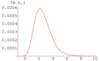
(a)   (b)

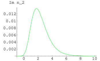
Figure 6: The behaviour of (a) $\text{Im}\,n_{1}(\omega)$ and (b) $\text{Im}\,n_{2}(\omega)$ in units of $\alpha R/(2\pi m^{2})$, as a function of $\tfrac{1}{2}\log\omega^{2}R/m^{4}$ for the Type II Ricci flat case.

Type II:   In this case, the integrand in (20) has branch point singularities on both the real and imaginary axes. The refractive indices therefore have both a real and imaginary part. These are shown figs. (5) and (6) for the special case of a Ricci flat background with $\sigma_{1}=i\sigma_{2}=\sqrt{R}$. Notice that the subluminal polarization state $n_{2}(\omega)$ has the same general form as the refractive index for a conventional absorptive optical medium [4, 2].

In this case the propagation displays gravitational bi-refringence [5, 24] since the two polarizations have different phase velocities. In general, the low-frequency limit of the refractive index is

$$n_{i}(\omega)=1-\frac{\alpha}{360\pi}{1\over m^{2}}\big{(}10\Phi_{00}\mp 4|\Psi_{0}|\big{)}+{\cal O}(\omega^{2})\ .$$ (25)

for $i=1,2$. For Type II, at low frequencies, we find has

$$n_{1,2}(\omega)=1\mp\frac{\alpha R}{2\pi m^{2}}\Big{[}\frac{1}{45}\mp\frac{37}{28350}\frac{\omega^{2}R}{m^{4}}+\frac{34}{85995}\Big{(}\frac{\omega^{2}R}{m^{4}}\Big{)}^{2}\mp\cdots\Big{]}\ .$$ (26)

for the superluminal and subluminal polarizations respectively. In both cases the Borel transforms have branch point singularities on the real axis and this is indicative of an imaginary part which vanishes to all orders in the $\omega^{2}R/m^{4}$ expansion. In fact, for low frequencies, $\text{Im}\,n(\omega)$ is dominated by the closest singularity to the origin, leading to the universal behaviour

$$\text{Im}\,n_{i}(\omega)\thicksim\exp-\frac{2\pi m^{2}}{\omega|\sigma_{2}|}\ .$$ (27)

The high-frequency limit is again given by (24), where this time the $C_{i}$ are complex but still with $\text{Re}~{}C_{i}>0$, so that all polarizations for both Type I and Type II have phase velocities that approach $c$ at high frequencies from the superluminal side.

5 Micro-Causality and the Kramers-Kronig Relation

These results on the analyticity structure of $\Pi^{\text{1-loop}}(\omega)$ and $n(\omega)$ explain why the Kramers-Kronig dispersion relation fails to hold for QED in curved spacetime. The derivation of (1) relies on the fact that $n(\omega)$ is analytic in the upper-half plane. As we have seen, however, this is not true in curved spacetime because $n(\omega)$ has singularities on the imaginary axis (see fig. (7)) and these must be included in the contour integral used to derive (1). So, for example, in the conformally flat Type I case, the singularities are poles and we have

$$\begin{split}&\int_{\text{semi-circle}}\frac{d\omega}{\omega}\,n(\omega)-\pi in(0)+{\cal P}\int_{-\infty}^{\infty}\frac{d\omega}{\omega}\,n(\omega)\\ &=\pi i\big{(}n(\infty)-n(0)\big{)}+{\cal P}\int_{-\infty}^{\infty}\frac{d\omega}{\omega}\,n(\omega)~{}=~{}\text{pole contribution}\ .\end{split}$$ (28)

Figure 7: The integration contour for $\oint d\omega\,n(\omega)/\omega$ used in the proof of the generalized KK relation for the conformally flat symmetric wave with poles on the imaginary axis.

In this case $\text{Im}\,n(\omega)=0$ and the principal value integral vanishes, and (28) becomes

$$\text{Re}\,n(0)-\text{Re}\,n(\infty)=\frac{\alpha R}{\pi m^{2}}\int_{0}^{\infty}dT\,e^{-T}\,\int_{0}^{1}d\xi\,\big{(}\xi(1-\xi)\big{)}^{2}\,\sum_{n=1}^{\infty}\text{Res}\,f(i\pi n/2)\ ,$$ (29)

where $f(x)=\big{(}1-\tfrac{x^{4}}{\sinh^{4}x\cosh^{2}x}\big{)}\tfrac{1}{x^{3}}$. Performing the residue sum we find

$$\text{Re}\,n(0)-\text{Re}\,n(\infty)=-\frac{\alpha R}{36\pi m^{2}}\ ,$$ (30)

which is in perfect agreement with (23) and (24).

The fact that $n(\omega)$ is not analytic in the upper-half plane calls into question the validity of micro-causality. Recall that in relativistic QFT, micro-causality, i.e. the vanishing of commutators of field operators for spacelike separations, implies that the retarded propagator $\Delta_{\rm ret}$ is only non-vanishing in, or, as in the present case of a massless quantum, on, the forward null cone. At tree level, this remains true for QED in curved spacetime. However, at one loop, the vacuum polarization $\Pi_{ij}^{\text{1-loop}}$ contributes to the full propagator: $\Delta=\Delta^{\text{tree}}-\Delta^{\text{tree}}\Pi^{\text{1-loop}}\Delta^{\text{tree}}+\cdots$, and we must check whether $\Pi^{\text{1-loop}}$ itself only has support in/on the forward cone.

From our calculation of the on-shell momentum-space vacuum polarization tensor $\Pi^{\text{1-loop}}(\omega)$, we can attempt to determine the dependence of the real-space $\Pi^{\text{1-loop}}$ on the null coordinate $v$ by taking a Fourier transform:

$$\Pi^{\text{1-loop}}(v)=\int_{-\infty}^{\infty}d\omega\,e^{-i\omega v}\Pi^{\text{1-loop}}(\omega)\ .$$ (31)

This is a retarded quantity if the integration contour is taken to avoid singularities by veering into the upper-half plane, when $v<0$, and the lower half plane, when $v>0$. For QFT in flat spacetime, $\Pi^{\text{1-loop}}(\omega)$ is analytic in the upper-half plane and so when $v<0$ one computes the $\omega$ integral by completing the contour with a semi-circle at infinity in the upper-half plane. Since there are no singularities in the upper-half plane, the integral vanishes and consequently $\Pi^{\text{1-loop}}_{\text{ret}}(v)=0$ for $v<0$. This is consistent with the fact that the region $v<0$ lies outside the forward light cone. Hence, in this case micro-causality is preserved as a consequence of analyticity in the upper-half plane in frequency space.

In curved spacetime, on the contrary, $\Pi^{\text{1-loop}}(\omega)$ is not analytic in the upper-half plane and consequently $\Pi^{\text{1-loop}}_{\text{ret}}(v)$ may receive contributions from the region $v<0$ which lies outside the forward light cone. See fig. (8).

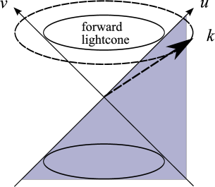
Figure 8: Including vacuum polarization effects, the photon momentum $k$ may lie outside the forward light cone ($u>0$, $v>0$) of its original null geodesic $v=0$. The potential violation of micro-causality arises if the retarded propagator is non-vanishing even for $v<0$ (the shaded area), which lies outside the forward light cone.

Indeed, for the conformally flat case where $\Pi^{\text{1-loop}}_{\text{ret}}(\omega)$ has poles on the imaginary axis, we can estimate the behaviour of $\Pi^{\text{1-loop}}_{\text{ret}}(v)$ as

$$\Pi^{\text{1-loop}}_{\text{ret}}(v)\thicksim\exp-\sqrt{\frac{8\pi m^{2}|v|}{R^{1/2}}}\ .$$ (32)

which appears to show a violation of micro-causality with an exponential dependence on a characteristic time/length scale $\sqrt{R}/m^{2}$.

However, in order to be certain that this is a genuine property of the full real-space propagator, it is necessary to calculate the vacuum polarization off-shell [26]. In our ${\cal O}(\alpha)$ on-shell calculation of $\Pi_{ij}$, the frequency $\omega$ is identified with the light-cone component $p_{+}$, while the component $p_{-}$ is taken to zero. It remains possible that when $p_{-}$ is small, but non-vanishing, the non-analyticities are shifted into the causally safe region $\text{Im}\,p_{+}/\text{Im}\,p_{-}<0$.

It will be especially interesting to explore these issues of superluminal propagation and causality in spacetimes such as Schwarzschild with both horizons and singularities. Although both $\Phi_{00}$ and $\Psi_{0}$ vanish for principal null geodesics at an event horizon, higher-order terms in the Penrose expansion do play a rôle and the non-vanishing of commutators in the neighbourhood of a horizon could have profound consequences. The UV-IR effect whereby high frequencies probe the global properties of the photon’s null geodesic could be especially important in spacetimes with singularities. We have implicitly assumed here that the null geodesics in the congruence are complete. However, this is no longer true in the presence of singularities, raising the intriguing possibility that their existence could affect the high frequency behaviour of photon propagation in a global rather than purely local way.

We would like to thank Asad Naqvi for many useful conversations and Sergei Dubovsky, Alberto Nicolis, Enrico Trincherini and Giovanni Villadoro for pointing out the necessity of working off-shell in order to completely settle the question of micro-causality. TJH would also like to thank Massimo Porrati for a helpful discussions and Fiorenzo Bastianelli for explaining some details of his work on the world-line formalism. This work was supported in part by PPARC grant PP/D507407/1.

References

- [1]
- [2] T.J. Hollowood and G.M. Shore, “The refractive index of curved spacetime: the fate of causality in QED,” arXiv:07072303 [hep-th]
- [3] G. M. Shore, Contemp. Phys. 44 (2003) 503 [arXiv:gr-qc/0304059].
- [4] G. M. Shore, Nucl. Phys. B 778 (2007) 219 [arXiv:hep-th/0701185].
- [5] I. T. Drummond and S. J. Hathrell, Phys. Rev. D 22 (1980) 343.
- [6] S. W. Hawking and G. F. R. Ellis, “The Large Scale Structure of Spacetime”, Cambridge University Press, 1973.
- [7] S. Liberati, S. Sonego and M. Visser, Annals Phys. 298 (2002) 167 [arXiv:gr-qc/0107091].
- [8] G. M. Shore, “Causality and Superluminal Light”, in ‘Time and Matter’, Proceedings of the International Colloquium on the Science of Time, Venice, ed. I. Bigi and M. Faessler, World Scientific, Singapore, 2006. [arXiv:gr-qc/0302116].
- [9] H. A. Kramers, Atti Congr. Intern. Fisici, Como, Nicolo Zanichelli, Bologna, 1927; reprinted in H. A. Kramers, Collected Scientific Papers, North-Holland, Amsterdam, 1956.
- [10] R. de Kronig, Ned. Tyd. Nat. Kunde 9 (1942) 402; Physica 12 (1946) 543.
- [11] S. Weinberg, “The Quantum Theory of Fields”, Vol I, Cambridge University Press, 1996.
- [12] R. P. Feynman, Phys. Rev. 80 (1950) 440.
- [13] J. S. Schwinger, Phys. Rev. 82 (1951) 914.
- [14] C. Schubert, Phys. Rept. 355 (2001) 73 [arXiv:hep-th/0101036].
- [15] F. Bastianelli and A. Zirotti, Nucl. Phys. B 642 (2002) 372 [arXiv:hep-th/0205182].
- [16] F. Bastianelli, O. Corradini and A. Zirotti, JHEP 0401 (2004) 023 [arXiv:hep-th/0312064].
- [17] F. Bastianelli, arXiv:hep-th/0508205.
- [18] H. Kleinert and A. Chervyakov, Phys. Lett. A 299 (2002) 319 [arXiv:quant-ph/0206022].
- [19] H. Kleinert and A. Chervyakov, Phys. Lett. A 308 (2003) 85 [arXiv:quant-ph/0204067].
- [20] M. Blau, D. Frank and S. Weiss, Class. Quant. Grav. 23 (2006) 3993 [arXiv:hep-th/0603109].
- [21] R. Penrose, “Any space-time has a plane wave as a limit,” in: Differential geometry and relativity, Reidel and Dordrecht (1976), 271-275.
- [22] M. Blau, “Plane waves and Penrose limits,” Lectures given at the 2004 Saalburg/Wolfersdorf Summer School, http://www.unine.ch/phys/string/Lecturenotes.html
- [23] R. M. Wald, “General Relativity”, Chicago University Press, 1984.
- [24] G. M. Shore, Nucl. Phys. B 460 (1996) 379 [arXiv:gr-qc/9504041].
- [25] G. M. Shore, Nucl. Phys. B 633 (2002) 271 [arXiv:gr-qc/0203034].
- [26] S. Dubovsky, A. Nicolis, E. Trincherini and G. Villadoro, “Microcausality in Curved Space-Time,” arXiv:0709.1483 [hep-th].
- [27] T.J. Hollowood and G.M. Shore, in preparation.
- [28]