Semiclassical Approach to Parametric Spectral Correlation with Spin 1/2

Abstract

The spectral correlation of a chaotic system with spin $1/2$ is universally described by the GSE (Gaussian Symplectic Ensemble) of random matrices in the semiclassical limit. In semiclassical theory, the spectral form factor is expressed in terms of the periodic orbits and the spin state is simulated by the uniform distribution on a sphere. In this paper, instead of the uniform distribution, we introduce Brownian motion on a sphere to yield the parametric motion of the energy levels. As a result, the small time expansion of the form factor is obtained and found to be in agreement with the prediction of parametric random matrices in the transition within the GSE universality class. Moreover, by starting the Brownian motion from a point distribution on the sphere, we gradually increase the effect of the spin and calculate the form factor describing the transition from the GOE (Gaussian Orthogonal Ensemble) class to the GSE class.

¹ Graduate School of Mathematics, Nagoya University, Chikusa-ku,
Nagoya 464-8602, Japan
² Department of Physics, Graduate School of Science, University of Tokyo, Hongo 7-3-1, Bunkyo-ku, Tokyo 113-0033, Japan

PACS: 05.45.Mt; 05.40.-a

KEYWORDS: quantum chaos; periodic orbit theory; random matrices

1 Introduction

The universal spectral correlation is one of the most outstanding features of quantum systems when the underlying classical dynamics is chaotic[1]. It is known that there are universality classes depending on the symmetry of the systems. For example, if time reversal invariance is broken, the corresponding spectral correlation is reproduced by the GUE (Gaussian Unitary Ensemble) of random matrices. On the other hand, the spectral correlation of the systems with time reversal invariance depends on the spin. If the system is spinless or has an integer spin, the GOE (Gaussian Orthogonal Ensemble) gives a precise prediction, while the GSE (Gaussian Symplectic Ensemble) applies to a system with a half odd spin.

In order to explain the universal behaviour from the underlying chaotic dynamics, much effort has been paid to establish a semiclassical theory of spectral correlations. The spectral form factor $K(\tau)$ (the Fourier transform of the spectral correlation function) is one of the most typical quantities of interest. Berry first succeeded in evaluating the leading term in the semiclassical $\tau$ expansion of the spectral form factor[2]. Then Sieber and Richter specified the classical orbit pairs which contribute to the second order term[3]. More recently Heusler et al. and Müller et al. extended Sieber and Richter’s work and calculate the full form of $K(\tau)$ in agreement with the prediction of random matrices[4, 5, 6, 7, 8].

In addition to each of the universality classes, the transitions within and among them are also of interest. The transitions are described by the spectral correlations depending on the transition parameters. It is conjectured that such parametric correlations are also reproduced by parametric extensions of random matrices[9, 10]. For the crossover from the GOE class to the GUE class, Saito and Nagao invented a scheme to incorporate the transition parameters into the semiclassical expansion of $K(\tau)$[11]. Similar schemes can also be applied to the transitions within the GUE and GOE classes[12, 13]. The agreements with parametric random matrices were in all cases confirmed.

In this paper, the parametric transition within the GSE symmetry class is treated. For that purpose, we shall study the spectral correlation of a chaotic system with spin $1/2$ by employing the strength of the effective field applied to the spin as the parameter. In order to simulate the spin dynamics, Brownian motion on the surface of a sphere is introduced. Using semiclassical periodic orbit theory, we evaluate the $\tau$ expansion of the spectral form factor up to the third order, so that the agreement with random matrix theory is confirmed. Moreover we study the crossover between a spinless system and a system with spin $1/2$. We suppose that the Brownian motion starts from a point distribution and that a diffusion on the sphere is caused by the increase of the coupling to the effective field. As a result, the semiclassical method yields the $\tau$ expansion of the form factor up to the second order.

The organization of this paper is as follows. In §2, semiclassical theory of a chaotic system with spin $1/2$ is developed. Assuming that the spin is coupled to a stochastic field, we explain how Brownian motion on a sphere arises. Then the leading term in the $\tau$ expansion of the form factor is evaluated by using Berry’s diagonal approximation. In §3, a diagrammatic method is introduced to calculate the higher order terms in the $\tau$ expansion. In §4, the prediction of random matrix theory is presented and compared with the semiclassical result. In §5, a similar semiclassical analysis is carried out for the crossover from a spinless system to a system with spin $1/2$. The last section is devoted to a brief summary.

2 Periodic Orbit Theory for a Chaotic System with Spin 1/2

Let us consider the energy level statistics of a bounded quantum system with $f$ degrees of freedom. Each phase space point is specified by a vector ${\bf x}=({\bf q},{\bf p})$, where $f$ dimensional vectors ${\bf q}$ and ${\bf p}$ give the position and momentum, respectively. It is assumed that the corresponding classical dynamics is chaotic ( homegeneously hyperbolic and ergodic). Moreover we suppose that the system has a spin with a fixed quantum number $S$. The strength of the interaction between the spin and effective field is characterized by a parameter $\eta$.

Let us denote by $E$ the energy of the system. Then, in the semiclassical limit $\hbar\to 0$, the energy level density $\rho(E;\eta)$ can be written in a decomposed form

$$\rho(E;\eta)\sim\rho_{\rm av}(E)+\rho_{\rm osc}(E;\eta).$$ (2.1)

Here $\rho_{\rm av}(E)$ is the local average of the level density, while $\rho_{\rm osc}(E;\eta)$ gives the fluctuation (oscillation) around the local average.

The local average of the level density is proportional to the number of Planck cells inside the energy shell:

$$\rho_{\rm av}(E)=(2S+1)\frac{\Omega(E)}{(2\pi\hbar)^{f}},$$ (2.2)

where the phase space volume with the energy between $E$ and $E+\Delta E$ is $\Omega(E)\Delta E$. The effective field is assumed to be so weak that $\rho_{\rm av}(E)$ does not depend on the parameter $\eta$.

On the other hand, in order to calculate the fluctuation part $\rho_{\rm osc}(E;\eta)$, we need to care about the time evolution of the spin. The spin state is described by a spinor with $2S+1$ elements and the spin evolution operator ${\hat{\Delta}}$ is represented by a $(2S+1)\times(2S+1)$ matrix. We denote such a representation matrix evaluated along the periodic orbit $\gamma$ by $\Delta_{\gamma}(\eta)$. Then, in the leading order of the semiclassical approximation, the fluctuation part of the level density is written as[6, 14, 15]

$$\rho_{\rm osc}(E;\eta)=\frac{1}{\pi\hbar}{\rm Re}\sum_{\gamma}({\rm tr}\Delta_{\gamma}(\eta))A_{\gamma}{\rm e}^{iS_{\gamma}(E)/\hbar}.$$ (2.3)

Here $S_{\gamma}$ is the classical action for the orbital motion, $A_{\gamma}$ is the stability amplitude (including the Maslov phase) and ${\rm tr}\Delta_{\gamma}(\eta)$ is the sum of the diagonal elements of $\Delta_{\gamma}(\eta)$.

Now we define the scaled parametric correlation function of the energy levels as

$$R(s;\eta,\eta^{\prime}) = \left\langle\frac{\rho\left(E+\frac{s}{2\rho_{\rm av}(E)};\eta\right)\rho\left(E-\frac{s}{2\rho_{\rm av}(E)};\eta^{\prime}\right)}{\rho_{\rm av}(E)^{2}}\right\rangle-1$$ (2.4)

$$\sim \left\langle\frac{\rho_{\rm osc}\left(E+\frac{s}{2\rho_{\rm av}(E)};\eta\right)\rho_{\rm osc}\left(E-\frac{s}{2\rho_{\rm av}(E)};\eta^{\prime}\right)}{\rho_{\rm av}(E)^{2}}\right\rangle.$$

Here we introduced averages depicted by the angular brackets $\langle\cdot\rangle$ over windows of the center energy $E$ and the scaled energy difference $s$. The form factor, namely the Fourier transform of $R(s;\eta,\eta^{\prime})$, is then written as

$$K(\tau;\eta,\eta^{\prime}) = \int_{-\infty}^{\infty}{\rm d}s\ {\rm e}^{i2\pi\tau s}R(s;\eta,\eta^{\prime})$$ (2.5)

$$\sim \left\langle\int{\rm d}\epsilon\ {\rm e}^{i\epsilon\tau T_{H}/\hbar}\frac{\rho_{\rm osc}\left(E+\frac{\epsilon}{2};\eta\right)\rho_{\rm osc}\left(E-\frac{\epsilon}{2};\eta^{\prime}\right)}{\rho_{\rm av}(E)}\right\rangle.$$

Here the angular brackets mean averages over windows of the center energy $E$ and the time variable $\tau$. Note that $\tau$ is measured in units of the Heisenberg time

$$T_{H}=2\pi\hbar\rho_{\rm av}(E)=(2S+1)\frac{\Omega(E)}{(2\pi\hbar)^{f-1}}.$$ (2.6)

It follows from (2.3) and (2.5) that the form factor is expressed as a double sum over periodic orbits

$$K(\tau;\eta,\eta^{\prime})\sim\frac{1}{T_{H}^{2}}\left\langle\sum_{\gamma,\gamma^{\prime}}({\rm tr}\Delta_{\gamma}(\eta))({\rm tr}\Delta_{\gamma^{\prime}}(\eta^{\prime}))^{*}A_{\gamma}A_{\gamma^{\prime}}^{*}{\rm e}^{i(S_{\gamma}-S_{\gamma^{\prime}})/\hbar}\delta\left(\tau-\frac{T_{\gamma}+T_{\gamma^{\prime}}}{2T_{H}}\right)\right\rangle,$$ (2.7)

where an asterisk stands for a complex conjugate. The periods of the periodic orbit $\gamma$ and its partner $\gamma^{\prime}$ are denoted by $T_{\gamma}$ and $T_{\gamma^{\prime}}$, respectively.

In principle, the spin evolution matrix $\Delta_{\gamma}(\eta)$ can be calculated from a deterministic equation of motion, if the Hamiltonian of the spin is explicitly known. However, here we take a simplified strategy based on an assumption that the spin evolution parameters undergo Brownian motion on the surface of a sphere[17]. The Brownian motion arises when the spin dynamics is determined by a stochastic Hamiltonian

$${\hat{\cal H}}=\eta({\bf h}\cdot{\hat{S}}),$$ (2.8)

where $\eta$ is an interaction-strength parameter and ${\hat{S}}$ is the spin operator. We assume that the components of the effective field

$${\bf h}=(h_{x}(t),h_{y}(t),h_{z}(t))$$ (2.9)

can be replaced by isotropic Gaussian white noises: denoting the average over the noises by the brackets $\langle\langle\cdot\rangle\rangle$, we find the correlation

$$\langle\langle h_{j}(t)h_{l}(t^{\prime})\rangle\rangle=0,\ \ \ j\neq l,$$

$$\langle\langle h_{j}(t)h_{j}(t^{\prime})\rangle\rangle=2D\delta(t-t^{\prime})$$ (2.10)

for $j,l=x,y,z$. Here isotropy implies that the diffusion constant $D$ does not depend on $j$.

The time evolution of the spin is described by a $(2S+1)\times(2S+1)$ matrix $\Delta(t)$ which satisfies the Schrödinger equation

$$i\hbar\frac{\partial}{\partial t}\Delta(t)={\cal H}\Delta(t),$$ (2.11)

where ${\cal H}$ is the matrix representation of the Hamiltonian ${\hat{\cal H}}$. Note that $\Delta(t)$ can be expressed as

$$\Delta(t)={\rm exp}\left(i\phi(t)S_{z}/\hbar\right){\rm exp}\left(i\theta(t)S_{x}/\hbar\right){\rm exp}\left(i\psi(t)S_{z}/\hbar\right),$$ (2.12)

where $S_{x}$ and $S_{z}$ are $(2S+1)\times(2S+1)$ matrices representing the $x$ and $z$ components of the spin operator ${\hat{S}}$. Thus three Euler angles $\psi$, $\theta$ and $\phi$ describe the spin evolution. Let us denote by $\chi({\cal T})$ a segment (with the duration ${\cal T}$) of the periodic orbit $\gamma$. When ${\cal T}$ coincides with the period, $\chi({\cal T})$ is equated with $\gamma$. Along such a segment $\chi({\cal T})$, the spin evolution matrix $\Delta_{\chi({\cal T})}$ is evaluated as

$$\Delta_{\chi({\cal T})}=\Delta({\cal T}).$$ (2.13)

Putting (2.12) into (2.11), we obtain the Langevin equation for the Euler angles

$${\dot{\phi}}/\eta = h_{x}\sin\phi\cot\theta+h_{y}\cos\phi\cot\theta-h_{z},$$

$${\dot{\theta}}/\eta = -h_{x}\cos\phi+h_{y}\sin\phi,$$

$${\dot{\psi}}/\eta = -h_{x}\sin\phi/\sin\theta-h_{y}\cos\phi/\sin\theta.$$ (2.14)

Then the Fokker-Planck equation

$$\frac{\partial P}{\partial t}=\eta^{2}D{\cal L}_{\rm SP}P$$ (2.15)

holds for the p.d.f.(probability distribution function) $P(\psi,\theta,\phi)$ with the measure $\sin\theta{\rm d}\psi{\rm d}\theta{\rm d}\phi$. Here

$${\cal L}_{\rm SP}=\frac{1}{\sin\theta}\frac{\partial}{\partial\theta}\sin\theta\frac{\partial}{\partial\theta}+\frac{1}{\sin^{2}\theta}\left(\frac{\partial^{2}}{\partial\psi^{2}}+\frac{\partial^{2}}{\partial\phi^{2}}-2\cos\theta\frac{\partial^{2}}{\partial\psi\partial\phi}\right)$$ (2.16)

is the Laplace-Beltrami operator on the sphere.

Let us suppose that the Euler angles $\psi$, $\theta$ and $\phi$ are equal to $\psi^{\prime}$,$\theta^{\prime}$ and $\phi^{\prime}$, respectively, when the interaction-strength parameter $\eta$ is zero. Then the solution of the Fokker-Planck equation gives the conditional p.d.f. of the Euler angles

$$g(\psi,\theta,\phi;t|\psi^{\prime},\theta^{\prime},\phi^{\prime})$$

$$= \sum_{j=0}^{\infty}\sum_{m=-j}^{j}\sum_{n=-j}^{j}\frac{2j+1}{32\pi^{2}}D^{j}_{m,n}(\psi,\theta,\phi)\left\{D^{j}_{m,n}(\psi^{\prime},\theta^{\prime},\phi^{\prime})\right\}^{*}{\rm e}^{-j(j+1)\eta^{2}Dt}.$$

Here $D^{j}_{m,n}$ is Wigner’s D function[18]

$$D^{j}_{m,n}(\psi,\theta,\phi)={\rm e}^{im\phi}d^{j}_{m,n}(\theta){\rm e}^{in\psi},$$ (2.18)

where

$$d^{j}_{m,n}(\theta)=\sqrt{\frac{(j+m)!(j-m)!}{(j+n)!(j-n)!}}\cos^{m+n}(\theta/2)\sin^{m-n}(\theta/2)P^{(m-n,m+n)}_{j-m}(\cos\theta)$$ (2.19)

with the Jacobi polynomials $P^{(a,b)}_{k}(x)$. Note that $j$ is an integer or a half odd integer ($j=0,1/2,1,3/2,\cdots$ and $m,n=-j,-j+1,\cdots,j$).

Under the assumption described above, the factor $({\rm tr}\Delta_{\gamma}(\eta))({\rm tr}\Delta_{\gamma^{\prime}}(0))$ in (2.7) with $\eta^{\prime}=0$ can be replaced by the average $\langle\langle\ ({\rm tr}\Delta_{\gamma}(\eta))({\rm tr}\Delta_{\gamma^{\prime}}(0))\ \rangle\rangle$ over the Brownian motion. Thus we can write the form factor as

$$K(\tau;\eta,0)$$

$$\sim \frac{1}{T_{H}^{2}}\left\langle\sum_{\gamma,\gamma^{\prime}}\langle\langle\ ({\rm tr}\Delta_{\gamma}(\eta))({\rm tr}\Delta_{\gamma^{\prime}}(0))^{*}\ \rangle\rangle A_{\gamma}A_{\gamma^{\prime}}^{*}{\rm e}^{i(S_{\gamma}-S_{\gamma^{\prime}})/\hbar}\delta\left(\tau-\frac{T_{\gamma}+T_{\gamma^{\prime}}}{2T_{H}}\right)\right\rangle.$$

We shall evaluate the $\tau$ expansion of this semiclassical form factor, focusing on the systems with spin $S=1/2$.

Let us calculate the leading term in the $\tau$ expansion by using Berry’s diagonal approximation[2]. In Berry’s approximation, one first considers the contributions from the pairs of identical periodic orbits $(\gamma,\gamma)$. The spin evolution matrix along $\gamma$ with $S=1/2$ is given by

$$\Delta_{\gamma}(\eta)={\rm exp}\left(\phi\frac{i}{2}\sigma_{z}\right){\rm exp}\left(\theta\frac{i}{2}\sigma_{x}\right){\rm exp}\left(\psi\frac{i}{2}\sigma_{z}\right),$$ (2.21)

where

$$\sigma_{x}=\left(\begin{array}[]{cc}0&1\\ 1&0\end{array}\right),\ \ \ \sigma_{z}=\left(\begin{array}[]{cc}1&0\\ 0&-1\end{array}\right)$$ (2.22)

are the Pauli matrices. It follows that

$${\rm tr}\Delta_{\gamma}(\eta)=2\cos\frac{\theta}{2}\cos\left\{\frac{1}{2}(\psi+\phi)\right\}.$$ (2.23)

The average of the factor $({\rm tr}\Delta_{\gamma}(\eta))({\rm tr}\Delta_{\gamma}(0))$ over the Brownian motion can be written as

$$\langle\langle\ ({\rm tr}\Delta_{\gamma}(\eta))({\rm tr}\Delta_{\gamma}(0))\ \rangle\rangle$$

$$= \int{\rm d}\omega{\rm d}\omega^{\prime}({\rm tr}\Delta_{\gamma}(\eta))({\rm tr}\Delta_{\gamma}(0))g(\psi,\theta,\phi;T|\psi^{\prime},\theta^{\prime},\phi^{\prime})p_{0}(\psi^{\prime},\theta^{\prime},\phi^{\prime}),$$

where $p_{0}$ is the p.d.f. of the Euler angles at $\eta=0$. The integrals are defined as

$$\int{\rm d}\omega = \int_{0}^{4\pi}{\rm d}\psi\int_{0}^{\pi}{\rm d}\theta\int_{0}^{4\pi}{\rm d}\phi\sin\theta,$$

$$\int{\rm d}\omega^{\prime} = \int_{0}^{4\pi}{\rm d}\psi^{\prime}\int_{0}^{\pi}{\rm d}\theta^{\prime}\int_{0}^{4\pi}{\rm d}\phi^{\prime}\sin\theta^{\prime}$$ (2.25)

and $T=T_{\gamma}$ is the period of $\gamma$.

For the transition within the GSE universality class (the GSE to GSE transition), we employ the uniform ”initial distribution”

$$p_{0}(\psi,\theta,\phi)=\frac{1}{32\pi^{2}},$$ (2.26)

since it yields the spectral form factor of the GSE class[6, 14, 15, 16]. The uniform distribution at $\eta=0$ implies that the spin is under the influence of additional interactions apart from the interaction described by (2.8). Putting (2.26) into (2), we obtain

$$\langle\langle\ ({\rm tr}\Delta_{\gamma}(\eta))({\rm tr}\Delta_{\gamma}(0))\ \rangle\rangle$$

$$= \frac{1}{32\pi^{2}}\int{\rm d}\omega{\rm d}\omega^{\prime}({\rm tr}\Delta_{\gamma}(\eta))({\rm tr}\Delta_{\gamma}(0))g(\psi,\theta,\phi;T|\psi^{\prime},\theta^{\prime},\phi^{\prime})$$

$$= \frac{1}{32\pi^{2}}\int{\rm d}\omega{\rm d}\omega^{\prime}\left\{D^{1/2}_{1/2,1/2}(\psi,\theta,\phi)+D^{1/2}_{-1/2,-1/2}(\psi,\theta,\phi)\right\}^{*}$$

$$\times\left\{D^{1/2}_{1/2,1/2}(\psi^{\prime},\theta^{\prime},\phi^{\prime})+D^{1/2}_{-1/2,-1/2}(\psi^{\prime},\theta^{\prime},\phi^{\prime})\right\}g(\psi,\theta,\phi;T|\psi^{\prime},\theta^{\prime},\phi^{\prime}).$$

Therefore, using the definition (2) of $g$ and the orthogonality relation

$$\int{\rm d}\omega\left\{D^{j}_{m,n}(\psi,\theta,\phi)\right\}^{*}D^{j^{\prime}}_{m^{\prime},n^{\prime}}(\psi,\theta,\phi)=\frac{32\pi^{2}}{2j+1}\delta_{j,j^{\prime}}\delta_{m,m^{\prime}}\delta_{n,n^{\prime}},$$ (2.28)

we can readily find

$$\langle\langle\ ({\rm tr}\Delta_{\gamma}(\eta))({\rm tr}\Delta_{\gamma}(0))\ \rangle\rangle={\rm e}^{-(3/4)aT}$$ (2.29)

with

$$a=\eta^{2}D.$$ (2.30)

Here the interaction-strength parameter $\eta$ is scaled so that $aT$ remains finite in the semiclassical limit $\hbar\rightarrow 0$. In order to take a step further, we need Hannay and Ozorio de Almeida (HOdA)’s sum rule[19]

$$\frac{1}{T_{H}^{2}}\left\langle\sum_{\gamma}\left|A_{\gamma}\right|^{2}\delta\left(\tau-\frac{T_{\gamma}}{T_{H}}\right)\right\rangle=\tau,$$ (2.31)

which results from the ergodicity of the system. Using this sum rule, we find the contribution to the form factor as

$$K_{(\gamma,\gamma)}(\tau;\eta,0) = \frac{1}{T_{H}^{2}}\left\langle\sum_{\gamma}\left|A_{\gamma}\right|^{2}\delta\left(\tau-\frac{T_{\gamma}}{T_{H}}\right)\right\rangle\langle\langle\ ({\rm tr}\Delta_{\gamma}(\eta))({\rm tr}\Delta_{\gamma}(0))\ \rangle\rangle$$ (2.32)

$$= \tau{\rm e}^{-(3/4)aT}.$$

The second contribution to Berry’s diagonal approximation comes from the pairs $(\gamma,{\bar{\gamma}})$, where a bar denotes time reversal. Noting

$$\Delta_{\bar{\gamma}}(\eta) = \{\Delta_{\gamma}(\eta)\}^{-1}$$ (2.37)

$$= \left(\begin{array}[]{cc}0&1\\ -1&0\end{array}\right)\left\{\Delta_{\gamma}(\eta)\right\}^{\rm T}\left(\begin{array}[]{cc}0&-1\\ 1&0\end{array}\right),$$

where $\left\{\Delta_{\gamma}(\eta)\right\}^{\rm T}$ is the transpose of $\Delta_{\gamma}(\eta)$, we find

$${\rm tr}\Delta_{\bar{\gamma}}(\eta)={\rm tr}\Delta_{\gamma}(\eta).$$ (2.38)

Therefore we can similarly obtain a contribution

$$K_{(\gamma,{\bar{\gamma}})}(\tau;\eta,0) = \frac{1}{T_{H}^{2}}\left\langle\sum_{\gamma}\left|A_{\gamma}\right|^{2}\delta\left(\tau-\frac{T_{\gamma}}{T_{H}}\right)\right\rangle\langle\langle\ ({\rm tr}\Delta_{\gamma}(\eta))({\rm tr}\Delta_{\bar{\gamma}}(0))\ \rangle\rangle$$ (2.39)

$$= \tau{\rm e}^{-(3/4)aT}.$$

Thus the total sum of the contributions to the diagonal approximation is

$$K_{\rm diag}(\tau)=K_{(\gamma,\gamma)}(\tau;\eta,0)+K_{(\gamma,{\bar{\gamma}})}(\tau;\eta,0)=2\tau{\rm e}^{-(3/4)aT}.$$ (2.40)

3 Off-diagonal Contributions

We are now in a position to calculate the off-diagonal contributions, restricting ourselves to the systems with two degrees of freedom ($f=2$). Encounters of periodic orbits play the major role in identifying the leading terms. An encounter is a set of orbit segments which come close to each other in the phase space. Long periodic orbits have encounters of the order of the Ehrenfest time $T_{E}$. In the semiclassical limit $\hbar\rightarrow 0$, $T_{E}$ logarithmically diverges. However, as the period $T$ is of the order of the Heisenberg time $T_{H}$, which more rapidly diverges, $T_{E}$ remains vanishingly small compared with the period. Therefore the periodic orbit mostly goes along loops in the phase space and occasionally visit encounters. As the leading terms are expected to result from the periodic orbit pairs $(\gamma,\gamma^{\prime})$ which are close to each other or mutually almost time reversed, we can suppose that $\gamma^{\prime}$ is almost identical to $\gamma$ or ${\bar{\gamma}}$ on the loops but differently connected in the encounters.

Let us consider such a periodic orbit pair $\alpha=(\gamma,\gamma^{\prime})$ in the phase space. Within each encounter, a Poincaré section ${\cal P}$ orthogonal to the orbit $\gamma$ can be introduced. Suppose that $\gamma$ pierces ${\cal P}$ within the $r$-th encounter. If $l_{r}$ segments of $\gamma$ are contained in the $r$-th encounter, there are $l_{r}$ piercing points on ${\cal P}$. The displacement $\delta{\bf x}$ between such points can be spanned as $\delta{\bf x}=s{\hat{e}}_{s}+u{\hat{e}}_{u}$. Here pairwise normalised vectors ${\hat{e}}_{s}$ and ${\hat{e}}_{u}$ have directions along the stable and unstable manifolds, respectively. Therefore, if one reference piercing point is chosen as the origin, each of other piercing points is identified by a coordinate pair $(s,u)$. As a result, if $\gamma$ has $L$ loops and $V$ encounters, $\sum_{r=1}^{V}(l_{r}-1)=L-V$ coordinate pairs $(s_{j},u_{j})$, $j=1,2,\cdots,L-V$ are necessary to identify the piercing points of $\gamma$.

Let us denote by $T_{j}$ the duration on the $j$-th loop and by $t_{r}$ the duration of the $r$-th encounter. Then the total duration of the encounters is

$$t_{\alpha}\equiv\sum_{r=1}^{V}l_{r}t_{r}$$ (3.1)

and the period is

$$T=\sum_{j=1}^{L}T_{j}+t_{\alpha}.$$ (3.2)

Ergodicity can be employed to estimate the number of encounters as[5, 6, 7, 11]

$$\int{\rm d}{\bf u}{\rm d}{\bf s}\int_{0}^{T-t_{\alpha}}{\rm d}T_{1}\int_{0}^{T-t_{\alpha}-T_{1}}{\rm d}T_{2}\cdots\int_{0}^{T-t_{\alpha}-T_{1}-T_{2}-\cdots-T_{L-2}}{\rm d}T_{L-1}\ Q_{\alpha},$$ (3.3)

where the integration measures are given by

$${\rm d}{\bf u}=\prod_{j=1}^{L-V}{\rm d}u_{j},\ \ \ {\rm d}{\bf s}=\prod_{j=1}^{L-V}{\rm d}s_{j}$$ (3.4)

and

$$Q_{\alpha}=\frac{T}{N_{\alpha}\ \prod_{r=1}^{V}t_{r}\ \Omega^{L-V}}.$$ (3.5)

Here $N_{\alpha}$ is a combinatorial factor chosen such that overcountings are avoided.

Now the contribution to the form factor from the orbit pair $\alpha=(\gamma,\gamma^{\prime})$ and its counterpart $(\gamma,{\bar{\gamma}^{\prime}})$ can be readily derived. Referring to (2) and (3.3) and taking account of (2.38), we find that such a contribution is

$$K_{\alpha}(\tau) = 2\tau\int{\rm d}{\bf u}{\rm d}{\bf s}\int_{0}^{T-t_{\alpha}}{\rm d}T_{1}\int_{0}^{T-t_{\alpha}-T_{1}}{\rm d}T_{2}\cdots\int_{0}^{T-t_{\alpha}-T_{1}-T_{2}-\cdots-T_{L-2}}{\rm d}T_{L-1}$$ (3.6)

$$\times Q_{\alpha}\langle\langle\ ({\rm tr}\Delta_{\gamma}(\eta))({\rm tr}\Delta_{\gamma^{\prime}}(0))\ \rangle\rangle{\rm e}^{i\Delta S/\hbar},$$

where the action difference $\Delta S\equiv S_{\gamma}-S_{\gamma^{\prime}}$ is given by $\Delta S=\sum_{j=1}^{L-V}u_{j}s_{j}$[5, 6, 7].

In order to obtain a semiclassical result, we need to expand $K_{\alpha}(\tau)$ in $t_{r}$’s and extract the terms in which all $t_{r}$’s mutually cancel. Since extra factors $\hbar$ appear or rapid oscillations take place in the limit $\hbar\to 0$, the other terms should be neglected[5, 6, 7]. The off-diagonal contribution to the semiclassical form factor is thus derived as

$$K_{\rm off}(\tau)=\sum_{\alpha}\frac{2\tau^{2}T_{H}}{N_{\alpha}}\left(\frac{2}{T_{H}}\right)^{L-V}\left.\frac{\partial^{V}}{\partial t_{1}\partial t_{2}\cdots\partial t_{V}}\Phi(t_{1},t_{2},\cdots,t_{V})\right|_{t_{1}=t_{2}=\cdots=t_{V}=0},$$ (3.7)

where

$$\Phi(t_{1},t_{2},\cdots,t_{V})$$

$$= \int_{0}^{T-t_{\alpha}}{\rm d}T_{1}\int_{0}^{T-t_{\alpha}-T_{1}}{\rm d}T_{2}\cdots\int_{0}^{T-t_{\alpha}-T_{1}-T_{2}-\cdots-T_{L-2}}{\rm d}T_{L-1}$$

$$\times \langle\langle\ ({\rm tr}\Delta_{\gamma}(\eta))({\rm tr}\Delta_{\gamma^{\prime}}(0))\ \rangle\rangle.$$

3.1 Sieber-Richter Term

In this and next subsection we consider the $\tau$ expansion of the above formula (3.7). Mathematica was used to assist the computations. Each term of (3.7) is of order $\tau^{n}$ with $n=L-V+1$. Let us first consider the second order term ($n=2$). The relevant pairs $\alpha=(\gamma,\gamma^{\prime})$ has two loops ($L=2$) and one encounter $(V=1)$. Such periodic orbit pairs were identified by Sieber and Richter and thus called SR (Sieber-Richter) pairs[3]. An SR pair is schematically depicted in Figure 1.

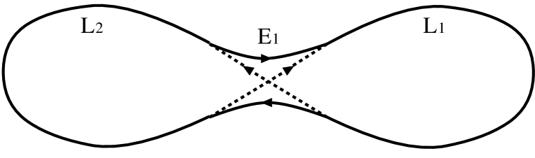
Figure 1: The periodic orbit pair contributing to the second order term

In Figure 1, $L_{1}$ and $L_{2}$ are loops and $E_{1}$ is an encounter. In the encounter, $\gamma$ and $\gamma^{\prime}$ are depicted by solid curves and dashed lines, respectively, and each arrow shows the direction of the motion. We can symbolically write the periodic orbits as

$$\gamma={\bar{E}_{1}}L_{2}E_{1}L_{1},\ \ \ \gamma^{\prime}={\bar{E}^{\prime}_{1}}{\bar{L}^{\prime}_{2}}E^{\prime}_{1}L^{\prime}_{1},$$ (3.9)

so that the spin evolution matrices are

$$\Delta_{\gamma}=(\Delta_{E_{1}})^{-1}\Delta_{L_{2}}\Delta_{E_{1}}\Delta_{L_{1}},\ \ \ \Delta_{\gamma^{\prime}}=(\Delta_{E^{\prime}_{1}})^{-1}(\Delta_{L^{\prime}_{2}})^{-1}\Delta_{E^{\prime}_{1}}\Delta_{L^{\prime}_{1}}.$$ (3.10)

A spin evolution matrix $\Delta_{\chi}$ along a segment $\chi$ of a periodic orbit is given by (2.13) and can be expressed as

$$\Delta_{\chi}={\rm exp}\left(\phi_{\chi}\frac{i}{2}\sigma_{z}\right){\rm exp}\left(\theta_{\chi}\frac{i}{2}\sigma_{x}\right){\rm exp}\left(\psi_{\chi}\frac{i}{2}\sigma_{z}\right)$$ (3.11)

in terms of a set of the Euler angles $\omega_{\chi}=(\psi_{\chi},\theta_{\chi},\phi_{\chi})$. The Pauli matrices $\sigma_{x}$ and $\sigma_{z}$ are defined in (2.22). The corresponding integral over the Euler angles is defined as

$$\int{\rm d}\omega_{\chi}=\int_{0}^{4\pi}{\rm d}\psi_{\chi}\int_{0}^{\pi}{\rm d}\theta_{\chi}\int_{0}^{4\pi}{\rm d}\phi_{\chi}\sin\theta_{\chi}.$$ (3.12)

Moreover we denote the durations of $L_{1}$, $L_{2}$ and $E_{1}$ by $T_{1}$, $T_{2}$ and $t_{1}$, respectively. Using the above notations, we evaluate the average of $({\rm tr}\Delta_{\gamma}(\eta))({\rm tr}\Delta_{\gamma^{\prime}}(0))$ as

$$\langle\langle\ ({\rm tr}\Delta_{\gamma}(\eta))({\rm tr}\Delta_{\gamma^{\prime}}(0))\ \rangle\rangle$$ (3.13)

$$= \frac{1}{(32\pi^{2})^{3}}\int{\rm d}\omega_{L_{1}}{\rm d}\omega_{L_{2}}{\rm d}\omega_{E_{1}}\int{\rm d}\omega_{L^{\prime}_{1}}{\rm d}\omega_{L^{\prime}_{2}}{\rm d}\omega_{E^{\prime}_{1}}$$

$$\times {\rm tr}((\Delta_{E_{1}})^{-1}\Delta_{L_{2}}\Delta_{E_{1}}\Delta_{L_{1}}){\rm tr}((\Delta_{E^{\prime}_{1}})^{-1}(\Delta_{L^{\prime}_{2}})^{-1}\Delta_{E^{\prime}_{1}}\Delta_{L^{\prime}_{1}})$$

$$\times g(\omega_{L_{1}};T_{1}|\omega_{L^{\prime}_{1}})g(\omega_{L_{2}};T-T_{1}-2t_{1}|\omega_{L^{\prime}_{2}})g(\omega_{E_{1}};t_{1}|\omega_{E^{\prime}_{1}})$$

$$= \frac{1}{4}{\rm e}^{-(3/4)aT}\left({\rm e}^{(3/2)at_{1}}-3{\rm e}^{-(1/2)at_{1}}\right),$$

so that

$$\Phi(t_{1})=\frac{T-2t_{1}}{4}{\rm e}^{-(3/4)aT}\left({\rm e}^{(3/2)at_{1}}-3{\rm e}^{-(1/2)at_{1}}\right).$$ (3.14)

Due to the equivalence of the segments $E_{1}$ and ${\bar{E}_{1}}$, we need to choose the combinatorial factor $N_{\alpha}$ as $N_{\rm SR}=2$[4]. Consequently we find the contribution from the SR pairs to the form factor as

$$K_{\rm SR}(\tau)=\frac{4\tau^{2}}{N_{\rm SR}}\left.\frac{\partial}{\partial t_{1}}\Phi(t_{1})\right|_{t_{1}=0}=2\tau^{2}{\rm e}^{-(3/4)aT}\left(1+\frac{3}{4}aT\right).$$ (3.15)

3.2 Third Order Term

Next we consider the third order term ($n=L-V+1=3$). It is known that the periodic orbit pairs contributing to the third order term are classified into five types: aas, api, ppi, ac and pc[4]. These five types are depicted in Figure 2.

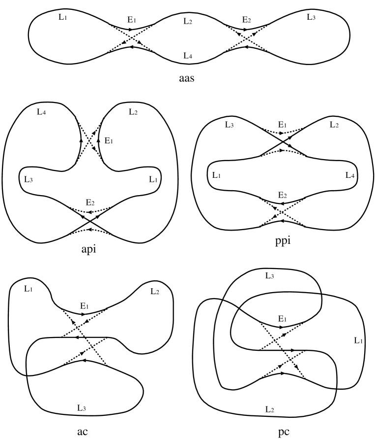
Figure 2: The periodic orbit pairs contributing to the third order term

As is seen from Figure 2, each of aas, api and ppi orbit pairs has four loops ($L=4$) and two encounters ($V=2$). The durations of the loops $L_{j}$ ($j=1,2,3,4$) and the encounters $E_{l}$ ($l=1,2$) are denoted by $T_{j}$ and $t_{l}$, respectively. The combinatorial factors $N_{\alpha}$ are known to be given by $N_{\rm aas}=2$, $N_{\rm api}=2$ and $N_{\rm ppi}=4$[4].

On the other hand, each of ac and pc orbit pairs has three loops ($L=3$) and one encounter ($V=1$). The times elapsed on the loops $L_{j}$ ($j=1,2,3$) and on the encounter $E_{1}$ are denoted by $T_{j}$ and $t_{1}$, respectively. The combinatorial factors $N_{\alpha}$ are $N_{\rm ac}=1$ and $N_{\rm pc}=3$[4].

In the following we calculate the contribution to the form factor $K_{\alpha}(\tau)$ from each of the five types: $\alpha={\rm aas},{\rm api},{\rm ppi},{\rm ac}$ and ${\rm pc}$.

(1) aas orbit pairs ($N_{\rm aas}=2$)

$$\langle\langle\ ({\rm tr}\Delta_{\gamma}(\eta))({\rm tr}\Delta_{\gamma^{\prime}}(0))\ \rangle\rangle$$ (3.16)

$$= \frac{1}{(32\pi^{2})^{6}}\int{\rm d}\omega_{L_{1}}{\rm d}\omega_{L_{2}}{\rm d}\omega_{L_{3}}{\rm d}\omega_{L_{4}}{\rm d}\omega_{E_{1}}{\rm d}\omega_{E_{2}}$$

$$\times \int{\rm d}\omega_{L^{\prime}_{1}}{\rm d}\omega_{L^{\prime}_{2}}{\rm d}\omega_{L^{\prime}_{3}}{\rm d}\omega_{L^{\prime}_{4}}{\rm d}\omega_{E^{\prime}_{1}}{\rm d}\omega_{E^{\prime}_{2}}$$

$$\times {\rm tr}(\Delta_{E_{1}}\Delta_{L_{2}}\Delta_{E_{2}}\Delta_{L_{3}}(\Delta_{E_{2}})^{-1}\Delta_{L_{4}}(\Delta_{E_{1}})^{-1}\Delta_{L_{1}})$$

$$\times {\rm tr}(\Delta_{E^{\prime}_{1}}(\Delta_{L^{\prime}_{4}})^{-1}\Delta_{E^{\prime}_{2}}\Delta_{L^{\prime}_{3}}(\Delta_{E^{\prime}_{2}})^{-1}(\Delta_{L^{\prime}_{2}})^{-1}(\Delta_{E^{\prime}_{1}})^{-1}\Delta_{L^{\prime}_{1}})$$

$$\times g(\omega_{L_{1}};T_{1}|\omega_{L^{\prime}_{1}})g(\omega_{L_{2}};T_{2}|\omega_{L^{\prime}_{2}})g(\omega_{L_{3}};T_{3}|\omega_{L^{\prime}_{3}})$$

$$\times g(\omega_{L_{4}};T-2t_{1}-2t_{2}-T_{1}-T_{2}-T_{3}|\omega_{L^{\prime}_{4}})$$

$$\times g(\omega_{E_{1}};t_{1}|\omega_{E^{\prime}_{1}})g(\omega_{E_{2}};t_{2}|\omega_{E^{\prime}_{2}})$$

$$= \frac{1}{16}{\rm e}^{-(3/4)aT}\left({\rm e}^{(3/2)at_{1}}-3{\rm e}^{-(1/2)at_{1}}\right)\left({\rm e}^{(3/2)at_{2}}-3{\rm e}^{-(1/2)at_{2}}\right).$$

Therefore

$$\Phi(t_{1},t_{2})$$

$$= \frac{(T-2t_{1}-2t_{2})^{3}}{96}{\rm e}^{-(3/4)aT}\left({\rm e}^{(3/2)at_{1}}-3{\rm e}^{-(1/2)at_{1}}\right)\left({\rm e}^{(3/2)at_{2}}-3{\rm e}^{-(1/2)at_{2}}\right),$$

so that

$$K_{\rm aas}(\tau) = \frac{8\tau^{2}}{N_{\rm aas}T_{H}}\left.\frac{\partial^{2}}{\partial t_{1}\partial t_{2}}\Phi(t_{1},t_{2})\right|_{t_{1}=t_{2}=0}$$ (3.18)

$$= 4\tau^{3}{\rm e}^{-(3/4)aT}\left\{1+\frac{3}{4}aT+\frac{3}{32}(aT)^{2}\right\}.$$

(2) api orbit pairs ($N_{\rm api}=2$)

$$\langle\langle\ ({\rm tr}\Delta_{\gamma}(\eta))({\rm tr}\Delta_{\gamma^{\prime}}(0))\ \rangle\rangle$$ (3.19)

$$= \frac{1}{(32\pi^{2})^{6}}\int{\rm d}\omega_{L_{1}}{\rm d}\omega_{L_{2}}{\rm d}\omega_{L_{3}}{\rm d}\omega_{L_{4}}{\rm d}\omega_{E_{1}}{\rm d}\omega_{E_{2}}$$

$$\times \int{\rm d}\omega_{L^{\prime}_{1}}{\rm d}\omega_{L^{\prime}_{2}}{\rm d}\omega_{L^{\prime}_{3}}{\rm d}\omega_{L^{\prime}_{4}}{\rm d}\omega_{E^{\prime}_{1}}{\rm d}\omega_{E^{\prime}_{2}}$$

$$\times {\rm tr}(\Delta_{E_{1}}\Delta_{L_{2}}\Delta_{E_{2}}\Delta_{L_{3}}\Delta_{E_{1}}\Delta_{L_{4}}(\Delta_{E_{2}})^{-1}\Delta_{L_{1}})$$

$$\times {\rm tr}(\Delta_{E^{\prime}_{1}}\Delta_{L^{\prime}_{2}}\Delta_{E^{\prime}_{2}}(\Delta_{L^{\prime}_{4}})^{-1}(\Delta_{E^{\prime}_{1}})^{-1}(\Delta_{L^{\prime}_{1}})^{-1}\Delta_{E^{\prime}_{2}}\Delta_{L^{\prime}_{3}})$$

$$\times g(\omega_{L_{1}};T_{1}|\omega_{L^{\prime}_{1}})g(\omega_{L_{2}};T_{2}|\omega_{L^{\prime}_{2}})g(\omega_{L_{3}};T_{3}|\omega_{L^{\prime}_{3}})$$

$$\times g(\omega_{L_{4}};T-2t_{1}-2t_{2}-T_{1}-T_{2}-T_{3}|\omega_{L^{\prime}_{4}})$$

$$\times g(\omega_{E_{1}};t_{1}|\omega_{E^{\prime}_{1}})g(\omega_{E_{2}};t_{2}|\omega_{E^{\prime}_{2}})$$

$$= \frac{1}{16}{\rm e}^{-(3/4)aT}\left({\rm e}^{(3/2)at_{1}}-3{\rm e}^{-(1/2)at_{1}}\right)\left({\rm e}^{(3/2)at_{2}}-3{\rm e}^{-(1/2)at_{2}}\right).$$

It follows that

$$K_{\rm api}(\tau)=4\tau^{3}{\rm e}^{-(3/4)aT}\left\{1+\frac{3}{4}aT+\frac{3}{32}(aT)^{2}\right\}.$$ (3.20)

(3) ppi orbit pairs ($N_{\rm ppi}=4$)

$$\langle\langle\ ({\rm tr}\Delta_{\gamma}(\eta))({\rm tr}\Delta_{\gamma^{\prime}}(0))\ \rangle\rangle$$ (3.21)

$$= \frac{1}{(32\pi^{2})^{6}}\int{\rm d}\omega_{L_{1}}{\rm d}\omega_{L_{2}}{\rm d}\omega_{L_{3}}{\rm d}\omega_{L_{4}}{\rm d}\omega_{E_{1}}{\rm d}\omega_{E_{2}}$$

$$\times \int{\rm d}\omega_{L^{\prime}_{1}}{\rm d}\omega_{L^{\prime}_{2}}{\rm d}\omega_{L^{\prime}_{3}}{\rm d}\omega_{L^{\prime}_{4}}{\rm d}\omega_{E^{\prime}_{1}}{\rm d}\omega_{E^{\prime}_{2}}$$

$$\times {\rm tr}(\Delta_{E_{1}}\Delta_{L_{2}}\Delta_{E_{2}}\Delta_{L_{3}}\Delta_{E_{1}}\Delta_{L_{4}}\Delta_{E_{2}}\Delta_{L_{1}})$$

$$\times {\rm tr}(\Delta_{E^{\prime}_{1}}\Delta_{L^{\prime}_{2}}\Delta_{E^{\prime}_{2}}\Delta_{L^{\prime}_{1}}\Delta_{E^{\prime}_{1}}\Delta_{L^{\prime}_{4}}\Delta_{E^{\prime}_{2}}\Delta_{L^{\prime}_{3}})$$

$$\times g(\omega_{L_{1}};T_{1}|\omega_{L^{\prime}_{1}})g(\omega_{L_{2}};T_{2}|\omega_{L^{\prime}_{2}})g(\omega_{L_{3}};T_{3}|\omega_{L^{\prime}_{3}})$$

$$\times g(\omega_{L_{4}};T-2t_{1}-2t_{2}-T_{1}-T_{2}-T_{3}|\omega_{L^{\prime}_{4}})$$

$$\times g(\omega_{E_{1}};t_{1}|\omega_{E^{\prime}_{1}})g(\omega_{E_{2}};t_{2}|\omega_{E^{\prime}_{2}})$$

$$= \frac{1}{16}{\rm e}^{-(3/4)aT}\left({\rm e}^{(3/2)at_{1}}-3{\rm e}^{-(1/2)at_{1}}\right)\left({\rm e}^{(3/2)at_{2}}-3{\rm e}^{-(1/2)at_{2}}\right).$$

It follows that

$$K_{\rm ppi}(\tau)=2\tau^{3}{\rm e}^{-(3/4)aT}\left\{1+\frac{3}{4}aT+\frac{3}{32}(aT)^{2}\right\}.$$ (3.22)

(4) ac orbit pairs ($N_{\rm ac}=1$)

$$\langle\langle\ ({\rm tr}\Delta_{\gamma}(\eta))({\rm tr}\Delta_{\gamma^{\prime}}(0))\ \rangle\rangle$$ (3.23)

$$= \frac{1}{(32\pi^{2})^{4}}\int{\rm d}\omega_{L_{1}}{\rm d}\omega_{L_{2}}{\rm d}\omega_{L_{3}}{\rm d}\omega_{E_{1}}\int{\rm d}\omega_{L^{\prime}_{1}}{\rm d}\omega_{L^{\prime}_{2}}{\rm d}\omega_{L^{\prime}_{3}}{\rm d}\omega_{E^{\prime}_{1}}$$

$$\times {\rm tr}(\Delta_{E_{1}}\Delta_{L_{1}}(\Delta_{E_{1}})^{-1}\Delta_{L_{2}}\Delta_{E_{1}}\Delta_{L_{3}}){\rm tr}(\Delta_{E^{\prime}_{1}}(\Delta_{L^{\prime}_{1}})^{-1}(\Delta_{E^{\prime}_{1}})^{-1}(\Delta_{L^{\prime}_{2}})^{-1}\Delta_{E^{\prime}_{1}}\Delta_{L^{\prime}_{3}})$$

$$\times g(\omega_{L_{1}};T_{1}|\omega_{L^{\prime}_{1}})g(\omega_{L_{2}};T_{2}|\omega_{L^{\prime}_{2}})g(\omega_{L_{3}};T-3t_{1}-T_{1}-T_{2}|\omega_{L^{\prime}_{3}})$$

$$\times g(\omega_{E_{1}};t_{1}|\omega_{E^{\prime}_{1}})$$

$$= \frac{1}{4}{\rm e}^{-(3/4)aT}\left(2{\rm e}^{-(3/2)at_{1}}-{\rm e}^{(3/2)at_{1}}\right).$$

Therefore

$$\Phi(t_{1})=\frac{(T-3t_{1})^{2}}{8}{\rm e}^{-(3/4)aT}\left(2{\rm e}^{-(3/2)at_{1}}-{\rm e}^{(3/2)at_{1}}\right),$$ (3.24)

so that

$$K_{\rm ac}(\tau)=\frac{8\tau^{2}}{N_{\rm ac}T_{H}}\left.\frac{\partial}{\partial t_{1}}\Phi(t_{1})\right|_{t_{1}=0}=-6\tau^{3}{\rm e}^{-(3/4)aT}\left(1+\frac{3}{4}aT\right).$$ (3.25)

(5) pc orbit pairs ($N_{\rm pc}=3$)

$$\langle\langle\ ({\rm tr}\Delta_{\gamma}(\eta))({\rm tr}\Delta_{\gamma^{\prime}}(0))\ \rangle\rangle$$ (3.26)

$$= \frac{1}{(32\pi^{2})^{4}}\int{\rm d}\omega_{L_{1}}{\rm d}\omega_{L_{2}}{\rm d}\omega_{L_{3}}{\rm d}\omega_{E_{1}}\int{\rm d}\omega_{L^{\prime}_{1}}{\rm d}\omega_{L^{\prime}_{2}}{\rm d}\omega_{L^{\prime}_{3}}{\rm d}\omega_{E^{\prime}_{1}}$$

$$\times {\rm tr}(\Delta_{E_{1}}\Delta_{L_{1}}\Delta_{E_{1}}\Delta_{L_{2}}\Delta_{E_{1}}\Delta_{L_{3}}){\rm tr}(\Delta_{E^{\prime}_{1}}\Delta_{L^{\prime}_{1}}\Delta_{E^{\prime}_{1}}\Delta_{L^{\prime}_{3}}\Delta_{E^{\prime}_{1}}\Delta_{L^{\prime}_{2}})$$

$$\times g(\omega_{L_{1}};T_{1}|\omega_{L^{\prime}_{1}})g(\omega_{L_{2}};T_{2}|\omega_{L^{\prime}_{2}})g(\omega_{L_{3}};T-3t_{1}-T_{1}-T_{2}|\omega_{L^{\prime}_{3}})$$

$$\times g(\omega_{E_{1}};t_{1}|\omega_{E^{\prime}_{1}})$$

$$= \frac{1}{4}{\rm e}^{-(3/4)aT}\left(2{\rm e}^{-(3/2)at_{1}}-{\rm e}^{(3/2)at_{1}}\right).$$

It follows that

$$K_{\rm pc}(\tau)=-2\tau^{3}{\rm e}^{-(3/4)aT}\left(1+\frac{3}{4}aT\right).$$ (3.27)

Putting the above results together, we obtain the third order contribution to the form factor

$$K_{\rm 3rd}(\tau) = K_{\rm aas}(\tau)+K_{\rm api}(\tau)+K_{\rm ppi}(\tau)+K_{\rm ac}(\tau)+K_{\rm pc}(\tau)$$ (3.28)

$$= 2\tau^{3}{\rm e}^{-(3/4)aT}\left\{1+\frac{3}{4}aT+\frac{15}{32}(aT)^{2}\right\}.$$

Hence the semiclassical form factor up to the third order is calculated from (2.40), (3.15) and (3.28) as

$$K_{\rm SC}(\tau) = K_{\rm diag}(\tau)+K_{\rm SR}(\tau)+K_{\rm 3rd}(\tau)$$

$$= 2\tau{\rm e}^{-(3/4)aT}\left[1+\left(1+\frac{3}{4}aT\right)\tau+\left\{1+\frac{3}{4}aT+\frac{15}{32}(aT)^{2}\right\}\tau^{2}\right].$$

4 Parametric Random Matrix Theory

Parametric random matrix theory was originally invented by Dyson[20]. The quantum Hamiltonian of a time reversal invariant system with spin $1/2$ is simulated by an $N\times N$ self-dual real quaternion random matrix $H$. It is assumed to be a sum of a self-dual real quaternion matrix $H_{0}$ and a Gaussian random perturbation: the p.d.f. of $H$ is given by

$$P(H;\sigma|H_{0})\ {\rm d}H\propto{\rm exp}\left[-2\frac{{\rm Tr}\left\{(H-{\rm e}^{-\sigma}H_{0})^{2}\right\}}{1-{\rm e}^{-2\sigma}}\right]{\rm d}H$$ (4.1)

with

$${\rm d}H=\prod_{j=1}^{N}{\rm d}H_{jj}\prod_{j<l}^{N}\prod_{k=0}^{3}{\rm d}H^{(k)}_{jl}.$$ (4.2)

Here $H^{(k)}_{jl}$ is the $k$-th component of the real quaternion $H_{jl}$. We are interested in the parametric motion of the matrix $H$ depending on the fictitious time parameter $\sigma$.

Let us write the eigenvalues of the self-dual real quaternion matrices $H$ and $H_{0}$ as $x_{1},x_{2},\cdots,x_{N}$ and $y_{1},y_{2},\cdots,y_{N}$, respectively. Dyson derived the Fokker-Planck equation

$$\frac{\partial p}{\partial\sigma}=\sum_{j=1}^{N}\frac{\partial}{\partial x_{j}}\left(\frac{\partial W}{\partial x_{j}}p+\frac{1}{4}\frac{\partial p}{\partial x_{j}}\right)$$ (4.3)

with

$$W=\frac{1}{2}\sum_{j=1}^{N}(x_{j})^{2}-\sum_{j<l}^{N}\log|x_{j}-x_{l}|$$ (4.4)

for the p.d.f. $p$ of the eigenvalues of $H$.

We denote by

$$G(x_{1},x_{2},\cdots,x_{N};\sigma|y_{1},y_{2},\cdots,y_{N})$$ (4.5)

the Green function solution of the Fokker-Planck equation (4.3). Namely, $G$ with the measure $\prod_{j=1}^{N}{\rm d}x_{j}$ gives the p.d.f. of the eigenvalues of $H$ at $\sigma$ under the condition that $x_{j}=y_{j}$ ($j=1,2,\cdots,N$) at $\sigma=0$. The limit $\sigma\to\infty$ of the Green function is given by the p.d.f. of the GSE eigenvalues

$$G(x_{1},x_{2},\cdots,x_{N};\infty|y_{1},y_{2},\cdots,y_{N})=p_{\rm GSE}(x_{1},x_{2},\cdots,x_{N}),$$ (4.6)

where

$$p_{\rm GSE}(x_{1},x_{2},\cdots,x_{N})\propto{\rm e}^{-4W}.$$ (4.7)

Let us choose the initial matrix $H_{0}$ as a GSE random matrix. Then the transition within the GSE symmetry class (the GSE to GSE transition) is realized. We define the dynamical (density-density) correlation function describing the correlation between the eigenvalues of $H$ and $H_{0}$ as

$$\kappa(x;\sigma|y)=N^{2}\frac{I(x;\sigma|y)}{I_{0}},$$ (4.8)

where

$$I(x_{1};\sigma|y_{1}) = \int_{-\infty}^{\infty}{\rm d}x_{2}\int_{-\infty}^{\infty}{\rm d}x_{3}\cdots\int_{-\infty}^{\infty}{\rm d}x_{N}\int_{-\infty}^{\infty}{\rm d}y_{2}\int_{-\infty}^{\infty}{\rm d}y_{3}\cdots\int_{-\infty}^{\infty}{\rm d}y_{N}$$

$$\times G(x_{1},x_{2},\cdots,x_{N};\sigma|y_{1},y_{2},\cdots,y_{N})p_{\rm GSE}(y_{1},y_{2},\cdots,y_{N})$$

and

$$I_{0}=\int_{-\infty}^{\infty}{\rm d}x\int_{-\infty}^{\infty}{\rm d}yI(x;\sigma|y).$$ (4.10)

The asymptotic limit $N\to\infty$ of the dynamical correlation function was evaluated by the method of supersymmetry[21]. It can also be derived by using the properties of the Jack symmetric polynomials[22]. Let us note that the asymptotic eigenvalue density at $\sqrt{2N}z$ ($-1<z<1$) is given by $\rho=\sqrt{2N(1-z^{2})}/\pi$. In terms of the new scaled variables $c,X$ and $Y$ defined as

$$\sigma=c/(\pi^{2}\rho^{2}),\ \ \ x=\sqrt{2N}z+(X/\rho),\ \ \ y=\sqrt{2N}z+(Y/\rho),$$ (4.11)

one obtains the asymptotic limit

$$\frac{\kappa(x;\sigma|y)}{\rho^{2}}-1\sim{\bar{\rho}}(\xi;c)$$ (4.12)

$$\equiv \frac{1}{2}\int_{1}^{\infty}{\rm d}u\int_{-1}^{1}{\rm d}v_{1}\int_{-1}^{1}{\rm d}v_{2}\frac{(u^{2}-1)(u-v_{1}v_{2})^{2}}{\{2uv_{1}v_{2}-u^{2}-(v_{1})^{2}-(v_{2})^{2}+1\}^{2}}$$

$$\times {\rm e}^{-c\{u^{2}+(v_{1})^{2}+(v_{2})^{2}-2(v_{1})^{2}(v_{2})^{2}-1\}}\cos\{2\pi\xi(u-v_{1}v_{2})\}$$

with $\xi=X-Y$. The Fourier transform of the asymptotic limit

$$K_{\rm RM}(\tau)=\int_{-\infty}^{\infty}{\rm d}\xi\ {\rm e}^{i2\pi\tau\xi}\ {\bar{\rho}}(\xi;c)$$ (4.13)

gives the definition of the form factor. It can be written as

$$K_{\rm RM}(\tau) = \frac{\tau^{2}}{2}\int_{1-\tau}^{1}{\rm d}v_{1}\int_{(1-\tau)/v_{1}}^{1}{\rm d}v_{2}$$ (4.14)

$$\times \frac{(v_{1}v_{2}+\tau)^{2}-1}{\{2(v_{1}v_{2}+\tau)v_{1}v_{2}-(v_{1}v_{2}+\tau)^{2}-(v_{1})^{2}-(v_{2})^{2}+1\}^{2}}$$

$$\times {\rm e}^{-c\{(v_{1}v_{2}+\tau)^{2}+(v_{1})^{2}+(v_{2})^{2}-2(v_{1})^{2}(v_{2})^{2}-1\}}$$

for $0\leq\tau\leq 1$. In order to derive the $\tau$ expansion of $K_{\rm RM}(\tau)$, we introduce new integration variables $s_{1}$ and $s_{2}$ by

$$\lambda_{1}=1-\frac{\tau}{2}s_{1},\ \ \ \lambda_{1}\lambda_{2}=1-\frac{\tau}{2}s_{2}.$$ (4.15)

Then we find

$$K_{\rm RM}(\tau)=\frac{\tau}{8}\int_{0}^{2}{\rm d}s_{1}\int_{s_{1}}^{2}{\rm d}s_{2}\ {\rm exp}\left\{-2\lambda\left(1-\frac{\tau}{2}s_{2}\right)-\lambda\tau\right\}$$

$$\times {\rm exp}\left\{\lambda\tau\frac{\displaystyle\left(s_{1}-\frac{\tau}{4}(s_{1})^{2}\right)\left(-s_{1}+s_{2}+\frac{\tau}{4}(s_{1})^{2}-\frac{\tau}{4}(s_{2})^{2}\right)}{\displaystyle\left(1-\frac{\tau}{2}s_{1}\right)^{2}}\right\}$$

$$\times \frac{\displaystyle\left(1-\frac{\tau}{2}s_{1}\right)^{3}\left(2-\frac{\tau}{2}s_{2}+\tau\right)\left(1-\frac{s_{2}}{2}\right)}{\displaystyle\left\{\left(s_{1}-\frac{\tau}{4}(s_{1})^{2}\right)\left(-s_{1}+s_{2}+\frac{\tau}{4}(s_{1})^{2}-\frac{\tau}{4}(s_{2})^{2}\right)-\left(1-\frac{\tau}{2}s_{1}\right)^{2}\right\}^{2}},$$

where $\lambda=c\tau$. Thus we can readily calculate the $\tau$ expansion (with fixed $\lambda$) from the Taylor expansion of the integrand as

$$K_{\rm RM}(\tau)=\frac{\tau}{8}{\rm e}^{-2\lambda}\left\{4+(2+4\lambda)\tau+\left(1+2\lambda+\frac{10}{3}\lambda^{2}\right)\tau^{2}+\cdots\right\}.$$ (4.17)

In order to compare this result with the semiclassical formula, we need to take account of the Kramers degeneracy, which means that all the eigenvalues have multiplicity two due to time reversal symmetry. Inclusion of the degeneracy yields a modified form factor

$${\tilde{K}}_{\rm RM}(\tau) = 2K_{\rm RM}(2\tau)$$

$$= 2\tau{\rm e}^{-2\lambda}\left\{1+(1+2\lambda)\tau+\left(1+2\lambda+\frac{10}{3}\lambda^{2}\right)\tau^{2}+\cdots\right\}.$$

This is in agreement with the semiclassical formula (3.2) up to the third order with an identification $\lambda=(3/8)aT$.

5 The GOE to GSE Transition

If the spin evolution operator is represented by an identity matrix, the system is effectively spinless and the resulting spectral correlation belongs to the GOE universality class. Therefore, the crossover from the GOE class to the GSE class can be treated by introducing

$$p_{0}(\psi,\theta,\phi)=\delta(\psi)\delta(\cos\theta-1)\delta(\phi)$$ (5.1)

as the ”initial distribution” instead of (2.26). In this section we investigate the GOE to GSE transition, focusing on the form factor $K(\tau,\eta,\eta)$, where $\eta^{\prime}$ is equated with $\eta$.

As before, due to the relation (2.38), the contributions from the pairs $(\gamma,\gamma^{\prime})$ and $(\gamma,{\bar{\gamma}}^{\prime})$ are equal. Therefore, in order to calculate the form factor in the diagonal approximation, it suffices to treat the pairs $(\gamma,\gamma)$. The average over the Brownian motion can be evaluated as

$$\langle\langle\ ({\rm tr}\Delta_{\gamma}(\eta))^{2}\ \rangle\rangle$$ (5.2)

$$= \int{\rm d}\omega{\rm d}\omega^{\prime}({\rm tr}\Delta_{\gamma}(\eta))^{2}g(\psi,\theta,\phi;T|\psi^{\prime},\theta^{\prime},\phi^{\prime})p_{0}(\psi^{\prime},\theta^{\prime},\phi^{\prime}),$$

$$= \int{\rm d}\omega({\rm tr}\Delta_{\gamma}(\eta))^{2}g(\psi,\theta,\phi;T|0,0,0).$$

Noting

$$({\rm tr}\Delta_{\gamma}(\eta))^{2}=D^{0}_{0,0}(\psi,\theta,\phi)+D^{1}_{-1,-1}(\psi,\theta,\phi)+D^{1}_{0,0}(\psi,\theta,\phi)+D^{1}_{1,1}(\psi,\theta,\phi)$$ (5.3)

and the orthogonality relation (2.28), we can readily find

$$\langle\langle\ ({\rm tr}\Delta_{\gamma}(\eta))^{2}\ \rangle\rangle=1+3{\rm e}^{-2aT}.$$ (5.4)

Then, using the HOdA sum rule (2.31), we find the contribution to the form factor

$$K_{(\gamma,\gamma)}(\tau;\eta,\eta) = \frac{1}{T_{H}^{2}}\left\langle\sum_{\gamma}\left|A_{\gamma}\right|^{2}\delta\left(\tau-\frac{T_{\gamma}}{T_{H}}\right)\right\rangle\langle\langle\ ({\rm tr}\Delta_{\gamma}(\eta))^{2}\ \rangle\rangle$$ (5.5)

$$= \tau(1+3{\rm e}^{-2aT}),$$

so that the diagonal term arising from the pairs $(\gamma,\gamma)$ and $(\gamma,{\bar{\gamma}})$ is

$$K_{\rm diag}(\tau)=K_{(\gamma,\gamma)}(\tau;\eta,\eta)+K_{(\gamma,{\bar{\gamma}})}(\tau;\eta,\eta)=2\tau(1+3{\rm e}^{-2aT}).$$ (5.6)

Let us next consider the second order term. As before, it can be evaluated from the Sieber-Richter pair $(\gamma,\gamma^{\prime})$ in Figure 1. We compute the average of $({\rm tr}\Delta_{\gamma}(\eta))({\rm tr}\Delta_{\gamma^{\prime}}(\eta))$ over the Brownian motion as

$$\langle\langle\ ({\rm tr}\Delta_{\gamma}(\eta))({\rm tr}\Delta_{\gamma^{\prime}}(\eta))\ \rangle\rangle$$ (5.7)

$$= \int{\rm d}\omega_{L_{1}}{\rm d}\omega_{L_{2}}{\rm d}\omega_{E_{1}}$$

$$\times {\rm tr}((\Delta_{E_{1}})^{-1}\Delta_{L_{2}}\Delta_{E_{1}}\Delta_{L_{1}}){\rm tr}((\Delta_{E_{1}})^{-1}(\Delta_{L_{2}})^{-1}\Delta_{E_{1}}\Delta_{L_{1}})$$

$$\times g(\omega_{L_{1}};T_{1}|0,0,0)g(\omega_{L_{2}};T-T_{1}-2t_{1}|0,0,0)g(\omega_{E_{1}};t_{1}|0,0,0)$$

$$= -\frac{1}{2}+\frac{3}{2}{\rm e}^{-2aT+4at_{1}}+\frac{3}{2}{\rm e}^{-2aT+2aT_{1}+4at_{1}}+\frac{3}{2}{\rm e}^{-2aT_{1}}.$$

Then we can evaluate the contribution to the form factor

$$K_{\rm SR}(\tau) = \frac{4\tau^{2}}{N_{\rm SR}}\left.\frac{\partial}{\partial t_{1}}\left\{\int_{0}^{T-2t_{1}}{\rm d}T_{1}\langle\langle\ ({\rm tr}\Delta_{\gamma}(\eta))({\rm tr}\Delta_{\gamma^{\prime}}(\eta))\ \rangle\rangle\right\}\right|_{t_{1}=0}$$ (5.8)

$$= 2\tau^{2}\left\{1+(6aT-9){\rm e}^{-2aT}\right\}.$$

Thus we obtain the semiclassical form factor up to the second order

$$K_{\rm SC}(\tau) = K_{\rm diag}(\tau)+K_{\rm SR}(\tau)$$ (5.9)

$$= 2\tau(1+3{\rm e}^{-2aT})+2\tau^{2}\left\{1+(6aT-9){\rm e}^{-2aT}\right\}.$$

A random matrix model of the GOE to GSE transition was already formulated in [23, 24]. However, as far as the authors know, an asymptotic formula to be compared with the above result (5.9) has not been worked out. Therefore it can be regarded as a conjecture for one of the open problems in random matrix theory.

The corresponding random matrix model can be formulated by using Dyson’s p.d.f. (4.1). Here we need to suppose that the initial matrix $H_{0}$ is a GOE random matrix. Namely, the matrix elements of $H_{0}$ only have the $0$-th components and the p.d.f. of $H_{0}$ is

$$P_{\rm GOE}(H_{0}){\rm d}H_{0}\propto{\rm e}^{-(1/2){\rm Tr}(H_{0})^{2}}{\rm d}H_{0}$$ (5.10)

with

$${\rm d}H_{0}=\prod_{j=1}^{N}{\rm d}(H_{0})_{jj}\prod_{j<l}^{N}{\rm d}(H_{0})_{jl}.$$ (5.11)

It is well known that the form factor of the GOE eigenvalues is expanded as

$$K_{\rm GOE}(\tau)=2\tau-2\tau^{2}+\cdots.$$ (5.12)

Considering the Kramers degeneracy, one modifies it into

$${\tilde{K}}_{\rm GOE}(\tau)=2K_{\rm GOE}(2\tau)=8\tau-16\tau^{2}+\cdots,$$ (5.13)

which is in agreement with the corresponding case $a=0$ of the semiclassical result (5.9).

6 Summary

In this paper, the parametric spectral correlation of a chaotic system with spin $1/2$ was studied. The parameter was chosen to be the strength of the effective field applied to the spin. Using the semiclassical periodic orbit theory for the orbital motion and simulating the spin dynamics by Brownian motion on a sphere, we evaluated the parameter-dependent spectral form factor $K_{\rm SC}(\tau)$. The $\tau$ expansion of $K_{\rm SC}(\tau)$ was found to be in agreement with the prediction of random matrix theory up to the third order. Moreover a crossover from a spinless system was investigated and the $\tau$ expansion of the corresponding form factor was calculated up to the second order.

References

• [1] O. Bohigas, M.J. Giannoni and C. Schmit, Phys. Rev. Lett. 52 (1984) 1.
• [2] M.V. Berry, Proc. R. Soc. London A400 (1985) 229.
• [3] M. Sieber and K. Richter, Physica Scripta T90 (2001) 128.
• [4] S. Heusler, S. Müller, P. Braun and F. Haake, J. Phys. A37 (2004) L31.
• [5] S. Müller, S. Heusler, P. Braun, F. Haake and A. Altland, Phys. Rev. Lett. 93 (2004) 014103-1.
• [6] S. Müller, S. Heusler, P. Braun, F. Haake and A. Altland, Phys. Rev. E72 (2005) 046207.
• [7] S. Müller, Periodic-Orbit Approach to Universality in Quantum Chaos (doctoral thesis, Universität Duisburg-Essen, 2005), nlin.CD/0512058.
• [8] S. Heusler, S. Müller, A. Altland, P. Braun and F. Haake, Phys. Rev. Lett. 98 (2007) 044103.
• [9] G. Lenz and F. Haake, Phys. Rev. Lett. 65 (1990) 2325.
• [10] F. Haake, Quantum Signatures of Chaos (2nd edition, Springer, 2000).
• [11] K. Saito and T. Nagao, Phys. Lett. A352 (2006) 380.
• [12] T. Nagao, P. Braun, S. Müller, K. Saito, S. Heusler and F. Haake, J. Phys. A40 (2007) 47.
• [13] J. Kuipers and M. Sieber, J. Phys. A40 (2007) 935.
• [14] J. Bolte and S. Keppeler, J. Phys. A32 (1999) 8863.
• [15] S. Keppeler, Spinning Particles - Semiclassics and Spectral Statistics (Springer, 2003).
• [16] J. Bolte and J. Harrison, J. Phys. A36 (2003) L433.
• [17] P.M. Hogan and J.T. Chalker, J. Phys. A37 (2004) 11751.
• [18] L.D. Landau and E.M. Lifshitz, Quantum Mechanics (Non-relativistic Theory) (Course of Theoretical Physics, Volume 3, 3rd edition, Elsevier, 1977).
• [19] J.H. Hannay and A.M. Ozorio de Almeida, J. Phys. A17 (1984) 3429.
• [20] F.J. Dyson, J. Math. Phys. 3 (1962) 1191.
• [21] B.D. Simons, P.A. Lee and B.L. Altshuler, Phys. Rev. B48 (1993) 11450.
• [22] Z.N.C. Ha, Phys. Rev. Lett. 73 (1994) 1574.
• [23] P.W. Brouwer, X. Waintal and B.I. Halperin, Phys. Rev. Lett. 85 (2000) 369.
• [24] S. Adam, M.L. Polianski, X. Waintal and P.W. Brouwer, Phys. Rev. B66 (2002) 195412.