Entanglement magnification induced by local manipulations

Abstract

We study the entanglement capability of the evolution of a pair of qubits evolving under unitary dynamics, when the local dynamical parameters cannot be modified during the time-evolution. Unlike the fast local control regime, we find that local and non-local contributions to the dynamics are strictly interconnected. Moreover, it is possible to strongly increase the entanglement capability by suitably initializing the characteristic energies of the two parties.

Introduction.— A basic ingredient for the implementation of quantum technologies is the ability to control some fundamental processes involving a pair of qubits, that is, the capacity of influencing the dynamics of this system through external actions. When the interaction with the environment is negligible, the system dynamics is given by the family of unitary transformations $U_{t}$ generated by the total Hamiltonian $H_{T}=H_{1}+H_{2}+H_{I}$, where $H_{1}$, $H_{2}$ are one-qubit contributions, and $H_{I}$ represents the interaction. This term is responsible for the generation of the peculiar quantum correlations called entanglement. The growing interest in the quantum theories of information and computation is largely due to these correlations, and to their potential applications. Therefore, it is of fundamental relevance to characterize the entanglement, to understand its properties and to study the processes leading to its creation. The relevant quantities involved are determined by the specific physical realization of the qubits pair.

The standard control setting is the so-called Local Unitary control (LU), where the control operations act locally (they influence $H_{1}$ and $H_{2}$, not $H_{I}$). Moreover, motivated by the available technologies, it is usually assumed that these operations are performed instantaneously khan ; benn (e.g., by means of short laser pulses). An arbitrary unitary transformation $U_{t}$ can be written as

$$U_{t}=A_{n}\otimes B_{n}e^{-iHt_{n}}\cdots e^{-iHt_{2}}A_{1}\otimes B_{1}e^{-iHt_{1}}A_{0}\otimes B_{0},$$ (1)

representing a succession of entangling evolutions, acting for time intervals $t_{1}\ldots t_{n}$, interspersed by instantaneous local evolutions, represented by the $A_{i}$ and $B_{i}$ operators, that can be arbitrarily manipulated. In general $H\neq H_{I}$, since the physical interaction can be used to simulate the dynamics generated by a different non-local contribution benn . In (1), the non-local and local parts are mutually independent.

Other control schemes have been developed for unitary dynamics, inspired by different experimental scenarios. In particular, the results presented in this work are relevant for the indirect control methods, in which an auxiliary system (ancilla) is used to manipulate the target system through their mutual interaction roma2 ; fu .

In the framework of LU control, the processes involving the qubits pair have been widely investigated in the past years. For fast local controls, the time-optimal generation of entanglement has been considered in dur , using the idea of entanglement capability of the interaction. For an arbitrary unitary operator, the maximal achievable entanglement, and the corresponding uncorrelated initial state, have been characterized in krau . A geometrical characterization of the entangling gates has been given in zhan , in terms of the coefficients describing the entanglement production. Other relevant topics, not directly connected to the entanglement generation, have been discussed in the literature, as the simulation of non-local gates benn ; khan ; vida ; hamm ; hase , and the ability of transmitting classical as well as quantum information hamm .

Even if usually well justified, the expression (1) is only an approximation, since it involves instantaneous actions. In this work, we relax this assumption by considering the opposite regime, in which the controls cannot be modified during the time evolution. In this case, it is not possible to distinguish between independent local and non-local contributions, as in (1). It turns out that the entangling part of the dynamics inherits an explicit dependence on $H_{1}$ and $H_{2}$ as long as $[H_{1}+H_{2},H_{I}]\neq 0$. Local control and entangling dynamics become deeply interconnected, and this dependence can be used to manipulate the non-local part by means of local control. In this letter we derive the entanglement capability in this regime, and show that particular choices of the local parameters can highly increase it.

Our analysis complements previous results obtained under the fast LU control assumption. Moreover, it is of interest in the context of indirect control methods, where the entanglement between target and auxiliary systems is fundamental to perform manipulations, and the parameters of the ancilla have to be fixed accordingly.

Cartan decomposition of unitary operators.— We assume that the time-evolution of the pair of qubits is given by a family of unitary maps generated by the total Hamiltonian. A fundamental property, known as Cartan decomposition (or canonical decomposition), factorizes an arbitrary unitary operator $U\in U(4)$ as

$$U=LAK,$$ (2)

where $L,K\in SU(2)\otimes SU(2)$ are local operators, and $A=e^{a}$, with $a$ an element of the Cartan subalgebra of the Lie algebra $\mathfrak{u}(4)=span(i\sigma_{j}\otimes\sigma_{j},j=x,y,z)$, $\sigma_{j}$ the Pauli operators for the two subsystems. The only operator that can correlate the two systems is $A$, that is called the entangling part. $L$ is irrelevant when dealing with entanglement generation.

This decomposition clarifies the role of the 16 parameters entering an arbitrary unitary transformation $U(4)$: the local contributions are characterized by twelve of them, the composite evolution by three of them, and finally there is a not-relevant overall phase. In particular,

$$a=-i\sum_{j}\theta_{j}\sigma_{j}\otimes\sigma_{j}=-i\sum_{j}\lambda_{j}|j\rangle\langle j|,$$ (3)

where $\theta_{j}$ ($j=x,y,z$) and $\lambda_{j}$ ($j=1,\ldots 4$) are real constants embodying the entanglement capability of the channel. In (3), we have introduced the eigenvalues $\lambda_{j}$ and eigenvectors $|j\rangle$ of $a$ (the so-called magic basis hill , given by the Bell states up to total phases). We notice that the $\lambda_{j}$ are constrained by ${\rm Tr}\,a=0$, then they sum up to zero. It is always possible to rearrange the coefficients as $\frac{\pi}{4}\geqslant\theta_{x}\geqslant\theta_{y}\geqslant\theta_{z}\geqslant 0$, using their properties of symmetry ($\theta_{j}\rightarrow\frac{\pi}{2}-\theta_{j}$) and periodicity ($\theta_{j}\rightarrow\theta_{j}+k_{j}\frac{\pi}{2},k_{j}\in\mathbb{Z}$). The relation between the two families of parameters is given by

$$\lambda_{1}=\theta_{x}-\theta_{y}+\theta_{z},\qquad \lambda_{2}=-\theta_{x}+\theta_{y}+\theta_{z},$$ (4)

$$\lambda_{3}=-\theta_{x}-\theta_{y}-\theta_{z},\quad\, \lambda_{4}=\theta_{x}+\theta_{y}-\theta_{z}.$$

The aforementioned entanglement capability of the interaction is defined as $h=\theta_{x}+\theta_{y}$ (e.g. see dur ).

Notice that the decomposition (2) justifies the expression (1); the non-local part is fully parameterized by three real constants, independent of the local actions.

Dynamical evolution.— The most general Hamiltonian terms are given by

$$H_{1}=\omega_{1}\vec{n}\cdot\vec{\sigma}\otimes{\mathbb{I}},\qquad H_{2}=\omega_{2}{\mathbb{I}}\otimes\vec{m}\cdot\vec{\sigma},$$ (5)

$$H_{I}=\sum_{ij}c_{ij}\sigma_{i}\otimes\sigma_{j},\qquad\qquad$$

where $i$ and $j$ range over $\{x,y,z\}$, $\omega_{1}$ and $\omega_{2}$ are the characteristic energies of the two subsystems, $\vec{n}$ and $\vec{m}$ are real unit vectors, $\vec{\sigma}$ is the vector of Pauli matrices and the coefficients $c_{ij}$ form a real matrix. Without loss of generality, we will consider representations of the Pauli matrices, for the two subsystems, such that this matrix is diagonal, $c_{ij}=c_{i}\delta_{ij}$.

The local actions consist of arbitrary preparations of $\vec{n}$, $\vec{m}$, $\omega_{1}$, and $\omega_{2}$. In order to have manageable expressions, we assume that only the characteristic energies can be modified, and we fix $\vec{n}=\vec{m}=(0,0,1)$. We further consider $\omega_{i}\geqslant 0$, $i=1,2$. The Cartan decomposition of the unitary transformation $U_{t}$ acting on the system is written as

$$U_{t}=e^{-iH_{T}t}=L_{t}A_{t}K_{t},$$ (6)

and the dependence on time is made apparent. We are interested in the relevant contributions for the entanglement generation, that is $A_{t}$ and $K_{t}$. It is possible to compute

$$U_{t}=\left[\begin{array}[]{cccc}e^{-ic_{z}t}\varphi_{1}(t)&0&0&e^{-ic_{z}t}\varphi_{4}(t)\\ 0&e^{ic_{z}t}\varphi_{2}(t)&e^{ic_{z}t}\varphi_{3}(t)&0\\ 0&e^{ic_{z}t}\varphi_{3}(t)&e^{ic_{z}t}\varphi_{2}^{*}(t)&0\\ e^{-ic_{z}t}\varphi_{4}(t)&0&0&e^{-ic_{z}t}\varphi_{1}^{*}(t)\\ \end{array}\right]$$ (7)

where

$$\varphi_{1}(t) = \cos{\Omega_{1}t}-i\,\Bigl{(}\frac{\omega_{1}+\omega_{2}}{\Omega_{1}}\Bigr{)}\sin{\Omega_{1}t},$$

$$\varphi_{2}(t) = \cos{\Omega_{2}t}-i\,\Bigl{(}\frac{\omega_{1}-\omega_{2}}{\Omega_{2}}\Bigr{)}\sin{\Omega_{2}t},$$

$$\varphi_{3}(t) = -i\,\Bigl{(}\frac{c_{x}+c_{y}}{\Omega_{2}}\Bigr{)}\sin{\Omega_{2}t},$$

$$\varphi_{4}(t) = -i\,\Bigl{(}\frac{c_{x}-c_{y}}{\Omega_{1}}\Bigr{)}\sin{\Omega_{1}t},$$ (8)

with frequencies

$$\Omega_{1} = \sqrt{(c_{x}-c_{y})^{2}+(\omega_{1}+\omega_{2})^{2}},$$

$$\Omega_{2} = \sqrt{(c_{x}+c_{y})^{2}+(\omega_{1}-\omega_{2})^{2}}.$$ (9)

In order to find the terms of the decomposition (6), it is convenient to represent all the operators in the magic basis, in which the local contributions become orthogonal matrices $\tilde{L}_{t}$ and $\tilde{K}_{t}$, and the non-local part $\tilde{A}_{t}$ is diagonal,

$$\tilde{U}_{t}=\tilde{L}_{t}\tilde{A}_{t}\tilde{K}_{t}.$$ (10)

Since $\tilde{U}_{t}^{T}\tilde{U}_{t}=\tilde{K}_{t}^{T}\tilde{A}_{t}^{2}\tilde{K}_{t}$, it is possible to determine $\tilde{A}_{t}$ and $\tilde{K}_{t}$ by considering the eigenvalues and eigenvectors of this operator. Applying the same procedure to $\tilde{U}_{t}\tilde{U}_{t}^{T}$ it is possible to find also $\tilde{L}_{t}$, however this contribution is not relevant for the purposes of this paper. Denoting the eigensystem as

$$\tilde{U}_{t}^{T}\tilde{U}_{t}\vec{v}_{i}(t)=\varepsilon^{2}_{i}(t)\vec{v}_{i}(t),\quad i=1,\ldots,4,$$ (11)

we obtain

$$\varepsilon^{2}_{1,2}(t) = e^{2ic_{z}t}\Bigl{(}\chi_{1}(t)\pm i\,\sqrt{1-\chi_{1}^{2}(t)}\Bigr{)},$$

$$\varepsilon^{2}_{3,4}(t) = e^{-2ic_{z}t}\Bigl{(}\chi_{2}(t)\pm i\,\sqrt{1-\chi_{2}^{2}(t)}\Bigr{)},$$ (12)

where we have defined two real-valued functions,

$$\chi_{1}(t) = 1-2\,\Bigl{(}\frac{c_{x}+c_{y}}{\Omega_{2}}\Bigr{)}^{2}\sin^{2}{\Omega_{2}t},$$

$$\chi_{2}(t) = 1-2\,\Bigl{(}\frac{c_{x}-c_{y}}{\Omega_{1}}\Bigr{)}^{2}\sin^{2}{\Omega_{1}t}.$$ (13)

Since $-1\leqslant\chi_{i}(t)\leqslant 1$ ($i=1,2$), it is possible to check that $|\varepsilon_{i}(t)|=1$, $i=1,\ldots 4$. The corresponding (non-normalized) eigenvectors are given by

$$\vec{v}_{1,2}(t) = (\mu_{1}(t)\mp\nu_{1}(t),0,0,1)^{T},$$

$$\vec{v}_{3,4}(t) = (\mu_{2}(t)\mp\nu_{2}(t),0,0,1)^{T},$$ (14)

where

$$\mu_{1}(t)=\frac{\Omega_{2}}{\omega_{1}-\omega_{2}}\cot{\Omega_{2}t},\quad\mu_{2}(t)=\frac{\Omega_{1}}{\omega_{1}+\omega_{2}}\cot{\Omega_{1}t},$$ (15)

and $\nu_{i}(t)=\sqrt{1+\mu_{i}^{2}(t)}$, for $i=1,2$. The normalized eigenvectors form the rows of the matrix $\tilde{K}_{t}$.

The non-local part in the magic basis is given by

$$\tilde{A}_{t}=diag\bigl{(}\varepsilon_{i}(t),i=1,\ldots 4\bigr{)},$$ (16)

and, following equation (3), it is possible to write

$$\varepsilon_{j}(t)=e^{-i\lambda_{j}(t)},\quad j=1,\ldots 4.$$ (17)

Therefore the Cartan coefficients are given by

$$\lambda_{1,2}(t) = c_{z}t\pm\frac{1}{2}\arccos{\chi_{2}(t)},$$

$$\lambda_{3,4}(t) = -c_{z}t\mp\frac{1}{2}\arccos{\chi_{1}(t)},$$ (18)

and the expressions for the $\theta_{i}(t)$, $i=x,y,z$, can be obtained inverting (4). These parameters characterize at every time the non-local contribution to the dynamics. Unlike the arbitrarily fast LU control case, they are time-dependent real functions that contain an explicit dependence on the local controls through the parameters $\Omega_{1}$ and $\Omega_{2}$, unless $[H_{1}+H_{2},H_{I}]=0$. This condition is satisfied only in two cases: either $\omega_{1}=\omega_{2}=0$, or $c_{x}=c_{y}=0$. In both cases $\lambda_{j}(t)$ are linear in $t$ and independent of the local controls, since the local dynamics and the interaction become independent processes.

Finally, the relevant contributions can be rewritten in the original basis. The local term can be cast in the form

$$K_{t}=\left[\begin{array}[]{cccc}0&0&0&e^{-i\eta_{2}(t)}\\ 0&0&e^{i\eta_{1}(t)}&0\\ 0&e^{-i\eta_{1}(t)}&0&0\\ e^{i\eta_{2}(t)}&0&0&0\\ \end{array}\right]$$ (19)

where

$$\eta_{i}(t)=\sqrt{\frac{\nu_{i}(t)+\mu_{i}(t)}{\nu_{i}(t)-\mu_{i}(t)}},\qquad i=1,2.$$ (20)

The non-local contribution has the form

$$A_{t}=\frac{1}{2}\left[\begin{array}[]{cccc}\varepsilon_{2}(t)+\varepsilon_{3}(t)&0&0&\varepsilon_{2}(t)-\varepsilon_{3}(t)\\ 0&\varepsilon_{1}(t)+\varepsilon_{4}(t)&\varepsilon_{1}(t)-\varepsilon_{4}(t)&0\\ 0&\varepsilon_{1}(t)-\varepsilon_{4}(t)&\varepsilon_{1}(t)+\varepsilon_{4}(t)&0\\ \varepsilon_{2}(t)-\varepsilon_{3}(t)&0&0&\varepsilon_{2}(t)+\varepsilon_{3}(t)\\ \end{array}\right].$$ (21)

Entanglement capability and optimal input states.— We are now able to derive the entanglement capability $h(t)$ of $U_{t}$ and study its properties. Considering (Entanglement magnification induced by local manipulations), it is possible to obtain

$$h(t)=\frac{\pi}{2}\,k(t)+\frac{1}{2}\,s(t)\arccos{\chi_{i(t)}(t)},$$ (22)

where $k(t)$, $s(t)$ and $i(t)$ are piecewise continuous functions with values in $\mathbb{Z}$, $\{-1,1\}$, and $\{1,2\}$ respectively, such that the hierarchy relations among the $\theta_{j}(t)$ are fulfilled at every time $t$. The specific form of these functions is not relevant for the purposes of this work. The entanglement capability is a continuous function in $t$, with $0\leqslant h(t)\leqslant\frac{\pi}{2}$, and it depends on the local parameters $\omega_{1}$ and $\omega_{2}$ through the functions $\chi_{i}(t)$, $i=1,2$. The extremal points for $\chi_{i}(t)$ can be found from $\partial_{t}\chi_{i}(t)=\partial_{\omega_{1}}\chi_{i}(t)=\partial_{\omega_{2}}\chi_{i}(t)=0$, whose relevant solutions are

$$\omega_{1}\mp\omega_{2}=0,\qquad t=k\,\frac{\pi}{2\,(c_{x}\pm c_{y})},$$ (23)

where the upper sign holds for $i=1$, the lower for $i=2$, and $k\in\mathbb{Z}$. A typical dependence of $h(t)$ on $\omega_{1}$ and $\omega_{2}$ for a critical value of $t$ is represented in Fig. 1. The complicate peak-valley pattern is determined by the extremal points of the functions $\chi_{i}(t)$, according to (22). From (23), it can be seen that the initial preparation of the local parameters has a strong impact on the evolution of the entanglement capability. In general, a sudden change is observed when $\omega_{1}$ and $\omega_{2}$ match. This is consistent with the behavior of the purification process discussed in roma . In fact, the entangling capability of the evolution is fundamental in indirect control schemes.

Figure 1: Dependence on $\omega_{1}$ and $\omega_{2}$ of the entanglement capability $h(t)$, for the Ising interaction $c_{x}=1$, $c_{y}=c_{z}=0$, and $t=\frac{3}{2}\pi$. The main peaks of $h(t)$ correspond to $\omega_{1}=\omega_{2}$. The other peaks are related to the extremal points of $\chi_{i}(t)$ with respect to $\omega_{1}$ and $\omega_{2}$, and $t$ fixed.

An initial state $|\psi\rangle_{0}$ is transformed by the evolution in the usually entangled state $|\psi\rangle_{t}=U_{t}|\psi\rangle_{0}$. The maximal attainable entanglement depends on the entanglement capability as well as on the initial state. It is possible to characterize the set of the optimal input states by solving the equation

$$|\psi\rangle_{0}=K_{t}A_{t}^{\dagger}|\Psi\rangle,$$ (24)

where $|\Psi\rangle$ is an arbitrary maximally entangled state, $K_{t}$ and $A_{t}$ are expressed in (19) and (21) respectively, and $K_{t}^{\dagger}=K_{t}$.

Conclusions.— When a two-qubits system is manipulated via local controls, it is usually assumed that these actions can be performed in an arbitrarily small time. Under this hypothesis, there is a clear separation between local and non-local contributions in the dynamics. The entangling capability of the evolution is a constant embodying the interaction content of the dynamics, and every initial factor state can produce the maximal amount of entanglement, since it can be instantaneously transformed, by fast local actions, in the optimal input state for the entanglement generation.

In this paper we have explored the entanglement generation in the opposite situation, where the local actions are fixed during the evolution. We have found that, in this regime, the local and non-local parts of the dynamics are strictly interconnected. Considering a particular control model, we have found the expression of the entanglement capability on the evolution time $t$, and on the local parameters $\omega_{1}$, $\omega_{2}$. In particular, $h(t)$ reaches its global maxima periodically in $t$, under the condition $\omega_{1}=\omega_{2}$. Only some selected input states maximize the entanglement production.

If less restrictive control models are adopted, in general it is not possible to obtain simple analytical expressions for the entanglement capability. However, there is strong evidence that the main features of the behavior of $h(t)$, described in this work, do not depend on the particular choice of $\vec{n}$ and $\vec{m}$. In fact, we have numerically computed $h(t)$ for a large sample of Hamiltonian operators, with randomly distributed values of $c_{x}$, $c_{y}$, $c_{z}$, $\vec{n}$ and $\vec{m}$. We have always found results that are consistent with the analysis presented in this work, in particular the insurgence of the peak of $h(t)$ when the two characteristic energies match. An prototypical example of these simulations is presented in Fig. 2, that exhibits the behavior of $h(t)$ for a particular evolution with $\vec{n}\neq\vec{m}$. The increase of $h(t)$ in correspondence of $\omega_{1}=\omega_{2}$ is not an artifact of the choice of the Hamiltonian terms assumed in this work, it is rather a general phenomenon in the two-qubits system.

The author acknowledges support from the European grant ERG:044941-STOCH-EQ. Work in part supported by Istituto Nazionale di Fisica Nucleare, Sezione di Trieste, Italy.

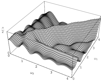
Figure 2: Dependence on $\omega_{1}$ and $\omega_{2}$ of the entanglement capability $h(t)$, with $c_{x}=-0.2$, $c_{y}=0.5$, $c_{z}=-0.8$, $t=3.7$, and $\vec{n}$ and $\vec{m}$ are the unit vectors corresponding to $(1,-3,2)$ and $(-2,1,4)$ respectively. The condition $\omega_{1}=\omega_{2}$ still plays a special role.

References

- (1) N. Khaneja, R. Brockett, and S.J. Glaser, Phys. Rev. A 63, 032308 (2001)
- (2) C.H. Bennett, J.I. Cirac, M.S. Leifer, D.W. Leung, N. Linden, S. Popescu and G. Vidal, Phys. Rev. A 66, 012305 (2002)
- (3) R. Romano and D. D’Alessandro, Phys. Rev. A 73, 022323 (2006), Phys. Rev. Lett. 97, 080402 (2006)
- (4) H.C. Fu, H. Dong, X.F. Liu and C.P. Sun, Phys. Rev. A 75, 052317 (2007)
- (5) W. Dür, G. Vidal, J.I. Cirac, N. Linden and S. Popescu, Phys. Rev. Lett. 87, 137901 (2001)
- (6) B. Kraus and J.I. Cirac, Phys. Rev. A 63, 062309 (2001)
- (7) J. Zhang, J. Vala, S. Sastry and K. B. Whaley, Phys. Rev. A 67, 042313 (2003)
- (8) G. Vidal, K. Hammerer, and J.I. Cirac, Phys. Rev. Lett. 88, 237902 (2002)
- (9) K. Hammerer, G. Vidal, and J.I. Cirac, Phys. Rev. A 66, 062321 (2002)
- (10) H.L. Haselgrove, M.A. Nielsen, and T.J. Osborne, Phys. Rev. A 68, 042303 (2003)
- (11) S. Hill and W.K. Wootters, Phys. Rev. Lett. 78, 5022 (1997)
- (12) R. Romano, Phys. Rev. A 75, 024301 (2007)