Abstract

A class of semi-parametric hazard/failure rates with a bathtub shape is of interest. It does not only provide a great deal of flexibility over existing parametric methods in the modeling aspect but also results in a closed and tractable Bayes estimator for the bathtub-shaped failure rate (BFR). Such an estimator is derived to be a finite sum over two ${\bf S}$-paths due to an explicit posterior analysis in terms of two (conditionally independent) ${\bf S}$-paths. These, newly discovered, explicit results can be proved to be a Rao-Blackwellization of counterpart results in terms of partitions that are readily available by a specialization of James (2005)’s work. We develop both iterative and non-iterative computational procedures based on existing efficient Monte Carlo methods for sampling one single ${\bf S}$-path. Numerical simulations are given to demonstrate the practicality and the effectiveness of our methodology. Last but not least, two applications of the proposed method are discussed, of which one is about a Bayesian test for failure rates and the other is related to modeling with covariates.

1 Introduction

In reliability theory and survival analysis it is often important to understand a hazard rate (or failure rate) as it is interpreted as the propensity of failure of an item or death of a human being in the instant future given its survival until time $t$. There are a variety of shapes for the function, for example, constant, non-increasing, or non-decreasing, of which each corresponds to a different life distribution. In particular, a class of life distributions which corresponds to a bathtub-shaped failure rate (BFR) has received considerable attention as most electronic, eletromechanical, and mechanical products and human beings are subject to a high risk for failures/deaths initially in an “infant mortality” phase, then to a lower and constant risk in the so-called “useful life” period and finally to an increasing risk with time during the so-called “wearout” phase. Many parametric families of distributions for BFRs have been proposed over the last few decades. Most of which typically involving three or more parameters are based on mixtures or generalizations of some common probability distributions, such as exponential, gamma, Weibull and Pareto distributions; see Rajarshi and Rajarshi (1988) and Lai, Xie, and Murthy (2001, Section 4) for an extensive and collective review. For discussion of parametric models for other typical hazard functions, see Kalbfleisch and Prentice (1980) and Lawless (1982). Also see Singpurwalla (2006) for a comprehensive discussion on reliability and risk from a Bayesian perspective.

One of the contributions of the present paper is a closed and tractable nonparametric estimator of BFRs that serve as a viable estimator of any BFR and, hence, an alternative to most existing parametric inferences which suffer from intractability problems [Lawless (1982), Page 255] and often resort to extensive iterative procedure [Haupt and Schabe (1997)]. The literature on nonparametric estimation of BFRs is rather limited though there are some available testing procedures involving BFRs (see, for example, Bergman (1979), Aarset (1985) and Vaurio (1999)). Amman (1984) (see also Laud, Damien and Walker (2006)) studied a $U$-shaped process by combining two random processes, of which one is the increasing random hazard rates based on extended gamma processes firstly considered by Dykstra and Laud (1981) and the other one is the decreasing counterpart defined analogously. However, the combined process does not necessarily generate BFRs. Reboul (2005) introduced a data-driven nonparametric estimator of BFRs which, though is not in a closed form, can be computed by applying the “Pool Adjacent Violators Algorithm” (see Barlow, Bartholomew, Bremner, and Brunk (1972)). References on nonparametric inference of any of hazard, survivor, or cumulative hazard functions in survival analysis include, for instance, Kaplan and Meier (1958), Watson and Leadbetter (1964a,b), Nelson (1969), Doksum (1974), Susarla and Van Ryzin (1976), Aalen (1978), Ferguson and Phadia (1979), Tanner and Wong (1983), Yandell (1983), Lo and Weng (1989), Hjort (1990), Wolpert and Ickstadt (1998) and James (2005), among others; see Ghosh and Ramamoorthi (2003) for a review of works related to Bayesian nonparametrics, and see also Sinha and Dey (1997) for an extensive survey on semi-parametric modeling of survival data with presence of covariates.

In line with James (2005) who studied random hazard rates with general shapes expressible as $\lambda(x|\mu)=\int K(x,u)\mu(du),$ wherein $K(x,u)$ is a known positive measurable kernel on a Polish space $\mathcal{X}\times\mathcal{U}$ and $\mu$ is a completely random measure [Kingman (1967, 1993)] on $\mathcal{U}$ (see Lo and Weng (1989) for the case when $\mu$ is an extended/weighted gamma random measure), the present paper considers a semi-parametric family of hazard rates on ${\cal{H}}=(0,\infty)$ defined by, for $t,\theta\in{\cal{H}}$,

$$\lambda(t|\mu,\theta)=\int_{\cal{R}}[\mathbb{I}(t-\theta\leq u<0)+\mathbb{I}(0<u\leq t-\theta)]\mu(du),$$ (1)

where $\mathbb{I}(A)$ is the indicator function of a set $A$ and $\mu$ is a completely random measure on $\cal{R}=(-\infty,\infty)$. Argument of Brunner (1992) in constructing unimodal densities on the real line with mode $\theta$ based on the mixture representation of a monotone failure rate (MFR) considered by Lo and Weng (1989) applies and justifies that (1) gives an BFR on $\cal{H}$ with a minimum point, or a change point called by Mitra and Basu (1995), at $\theta\in\cal{H}$. Posterior consistency of these BFRs can be established following Drǎgichi and Ramamoorthi (2003) who showed the corresponding result for the class of MFRs discussed in Ho (2006a), a subclass of (1) when $\theta=0$ or $\theta=\infty$. Exploiting the fine structure of an indicator kernel, Ho (2006a) improves the readily available explicit posterior analysis in terms of partitions in James (2005, Section 4) by giving a tractable and less complex (see Brunner and Lo (1989)) characterization in terms of one ${\bf S}$-path for such MFRs, and shows that an efficiently designed algorithm for sampling an ${\bf S}$-path, called the accelerated path (AP) sampler, results in less variable Bayes estimates of the hazard compared to a partition-based algorithm introduced by James (2005) via numerical simulations. In this work, we show that all BFRs defined in (1) possess nice and special structures that naturally arise in relation to two conditionally independent ${\bf S}$-paths given $\theta$ in Section 2, rather than one in the case of MFRs; for an BFR there are two (possibly different) non-decreasing curves away from the change point $\theta$ in either direction, compared with only one such curve to the right of the origin for a non-decreasing hazard rate. In particular, an explicit characterization depending on two ${\bf S}$-paths possessed by all such BFRs, which are unprecedentedly available, generalizes the corresponding characterization of MFRs discussed in Ho (2006a) that depends on only one path, and, more importantly, yields a tractable Bayes estimator of BFRs as a finite sum over two ${\bf S}$-paths. Understanding these novel characterization and estimator for BFRs is of statistical importance; they can be shown to be a Rao-Blackwellization of the partition-based counterparts, suggesting that more parsimonious methods for inference, compared with partition-based methods introduced in James (2005), would be available if one could efficiently sample the two paths in this context. To approximate posterior quantities for models in (1), Section 3 proposes an iterative Monte Carlo procedure based on the AP sampler. Furthermore, extensions of a sequential importance sampling (SIS) [Kong, Liu, and Wong (1994) and Liu and Chen (1998)] scheme for sampling one path at a time are introduced. Numerical results of the method are given in Section 4 to demonstrate its practicality and effectiveness. Two applications of the methodology are given in the last two sections in which the proposed algorithms can be applied to approximate the posterior quantities of interest. A test of an MFR versus an BFR based on models in (1) is illustrated in Section 5. Section 6 shows that a two ${\bf S}$-path characterization also exists in modeling with covariates by a proportional hazards model.

2 Posterior analysis via two ${\bf S}$-paths

A class of random hazard rates with a bathtub shape on the half line ${\cal{H}}$, defined by (1), is of interest. The law of $\mu$ is uniquely characterized by the Laplace functional

$${\cal L}_{\mu}(g|\rho,\eta)=\exp\left[-\int_{\cal{R}}\int_{\cal{H}}\left(1-e^{-g(u)x}\right)\rho(dx|u)\eta(du)\right],$$ (2)

where $g$ is a non-negative function on $\cal{R}$ and $\rho(dx|u)\eta(du)$ is called the Lévy measure of $\mu$. Also, $\mu$ can be represented in a distributional sense as

$$\mu(du)=\int_{\cal{H}}x{\cal N}(dx,du),$$

where ${\cal N}(dx,du)$ is a Poisson random measure, taking on points $(x,u)$ in $\cal{H}\times\cal{R}$, with mean intensity measure

$$\mathbb{E}[{\cal N}(dx,du)]=\rho(dx|u)\eta(du),$$ (3)

such that $\int_{B}\int_{\cal{H}}\mbox{min}(x,1)\rho(dx|u)\eta(du)<\infty$ for any bounded set $B\in\cal{R}$.

Suppose we collect independent failure times ${\bf T}=(T_{1},\ldots,T_{N})$ from $N$ items with a common continuous life distribution which corresponds to an BFR with change point at $\theta$, specified by (1), until time $\tau$, so that $0<T_{1}<\cdots<T_{m}<\tau$ denote $m$ completely observed failure times, and $T_{m+1}=\cdots=T_{N}\equiv\tau$ are $N_{c}\equiv N-m$ number of right-censored times. Assuming a multiplicative intensity model discussed in Aalen (1975, 1978), the likelihood of the data ${\bf T}$ is proportional to

$$e^{-\mu(g_{\smash{\lower 0.5382pt\hbox{{\tiny$N$,{\tiny$\theta$}}}}})}\prod_{i=1}^{m}\int[\mathbb{I}(T_{i}-\theta\leq u_{i}<0)+\mathbb{I}(0<u_{i}\leq T_{i}-\theta)]\mu(du_{i}),$$ (4)

where

$$g_{\smash{\lower 1.50694pt\hbox{{\scriptsize$N$,{\scriptsize$\theta$}}}}}(u)=\int_{0}^{\tau}\left[\sum_{i=1}^{N}\mathbb{I}(T_{i}\geq t)\right][\mathbb{I}(t-\theta\leq u<0)+\mathbb{I}(0<u\leq t-\theta)]dt$$

is a piecewise linear function of $u$, and $\mu(g_{\smash{\lower 1.50694pt\hbox{{\scriptsize$N$,{\scriptsize$\theta$}}}}})=\int_{\cal{R}}g_{\smash{\lower 1.50694pt\hbox{{\scriptsize$N$,{\scriptsize$\theta$}}}}}(u)\mu(du)=\int_{0}^{\tau}\left[\sum_{i=1}^{N}\mathbb{I}(T_{i}\geq t)\right]\lambda(t|\mu,\theta)dt$ with $\sum_{i=1}^{N}\mathbb{I}(T_{i}\geq t)$ called the total time on test (TTT) transform [Barlow, Bartholomew, Bremner, and Brunk (1972)]. Define $f_{\smash{\lower 1.50694pt\hbox{{\scriptsize$N$,{\scriptsize$\theta$}}}}}(x,u)=g_{\smash{\lower 1.50694pt\hbox{{\scriptsize$N$,{\scriptsize$\theta$}}}}}(u)x$ for any $(x,u)\in(\cal{H},\cal{R})$ and assume that

$$\kappa_{\ell}(e^{-f_{\smash{\lower 0.5382pt\hbox{{\tiny$N$,{\tiny$\theta$}}}}}}\rho|u)=\int_{\cal{R}}x^{\ell}e^{-g_{\smash{\lower 0.5382pt\hbox{{\tiny$N$,{\tiny$\theta$}}}}}(u)x}\rho(dx|u)<\infty,$$ (5)

for any positive integer $\ell\leq m$ and a fixed $u\in\cal{R}$.

The posterior distribution of the pair $(\mu,\theta)$ in (1) given ${\bf T}$ with respect to any prior $\pi(d\theta)$ for $\theta\in\cal{H}$ can always be determined by the double expectation formula,

$$\mathbb{E}[h(\mu,\theta)|{\bf T}]=\mathbb{E}\{\mathbb{E}[h(\mu,\theta)|\theta,{\bf T}]|{\bf T}\}=\int_{\cal{H}}\int_{\mathcal{M}}h(\mu,\theta)\mathcal{P}(d\mu|\theta,{\bf T})\mathcal{P}(d\theta|{\bf T}),$$ (6)

where $h$ is any nonnegative or integrable function, $\mathcal{M}$ is the space of measures over $\cal{R}$, and, $\mathcal{P}(d\mu|\theta,{\bf T})$ and $\mathcal{P}(d\theta|{\bf T})$ denote the conditional distribution of $\mu$ given $(\theta,{\bf T})$ and the posterior distribution of $\theta$ given ${\bf T}$, respectively.

Let us first look at $\mathcal{P}(d\mu|\theta,{\bf T})$ and then discuss $\mathcal{P}(d\theta|{\bf T})$ later on. Suppose $0<\theta<\tau$, we can always assume that

$$(T_{1}-\theta,\ldots,T_{m}-\theta)={\bf Z}^{\theta}\cup{\bf Y}^{\theta}=(Z_{1}^{\theta},Z_{2}^{\theta},\ldots,Z_{m-n}^{\theta})\cup(Y_{1}^{\theta},Y_{2}^{\theta},\ldots,Y_{n}^{\theta}),$$ (7)

where $-\theta\equiv Z^{\theta}_{0}<Z_{1}^{\theta}<Z_{2}^{\theta}<\cdots<Z_{m-n}^{\theta}<Z^{\theta}_{m-n+1}\equiv 0$ and $0\equiv Y^{\theta}_{n+1}<Y_{n}^{\theta}<Y_{n-1}^{\theta}<\cdots<Y_{1}^{\theta}<Y^{\theta}_{0}\equiv\tau-\theta$ are referred to as negative and positive observations in the sequel. The relationship between these notation and the data ${\bf T}$ is illustrated in Figure 1, graphed together with the TTT transform. It is worthy of note that once a failure time $T_{i}$, $i=1,\ldots,m$, is completely observed and compared with the given $\theta$, the mixture hazard rates can be simplified as in one of two mutually exclusive situations specified by

$$\lambda(T_{i}|\mu,\theta)=\left\{\begin{array}[]{lll}\int\mathbb{I}(Z_{j}^{\theta}\leq u_{i}<0)\mu(du_{i}),&&T_{i}-\theta=Z_{j}^{\theta}<0,\\ \int\mathbb{I}(0<u_{i}\leq Y_{k}^{\theta})\mu(du_{i}),&&T_{i}-\theta=Y_{k}^{\theta}>0,\end{array}\right.$$ (8)

for $j=1,\ldots,m-n$ and $k=1,\ldots,n$. This also implies that the missing variable $u_{i}$ corresponding to $T_{i}$ in (4) is always greater (resp. smaller) than 0 if $T_{i}>~{}(\mbox{resp. }<)\theta$. This nice similification proves to be crucial in leading to the tractable path structure of BFRs in (1).

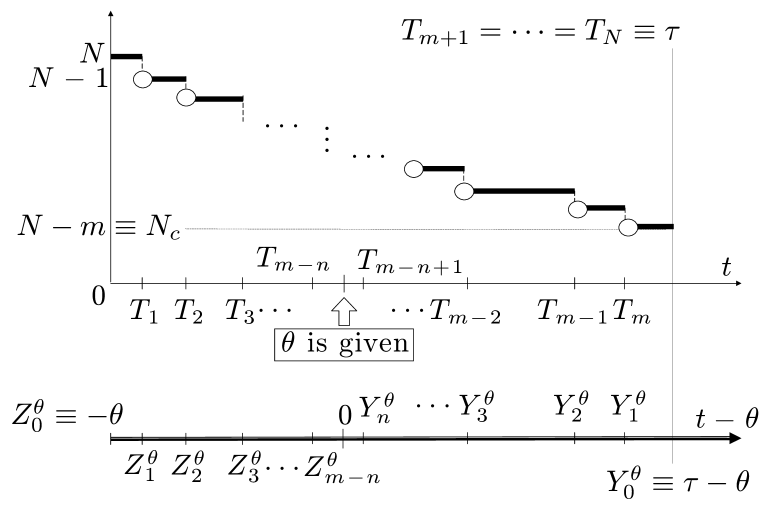
Figure 1:  Illustration of the TTT transform and the relationship (7) between ${\bf T}$ and $({\bf Y}^{\theta},{\bf Z}^{\theta},\theta)$.

Define an integer-valued vector ${\bf S}=(S_{0},S_{1},\ldots,S_{m-1},S_{m})$ [Lo and Weng (1989) and Brunner and Lo (1989)], referred to as an ${\bf S}$-path (of $m+1$ coordinates), which satisfies $S_{0}=0$, $S_{m}=m$ and $S_{j}\leq\min(j,S_{j+1})$, $j=1,\ldots,m-1$. An ${\bf S}$-path is a combinatorial reduction of a partition in the sense that an ${\bf S}$-path of $m+1$ coordinates is said to correspond to one or many partitions ${\bf p}=\{C_{1},\ldots,C_{n({\bf p})}\}$ of the integers $\{1,\ldots,m\}$, provided that (i) indices of the maximal elements of the $n({\bf p})$ cells $C_{k}$’s in ${\bf p}$ coincide with locations $j$ at which $S_{j}>S_{j-1}$, and (ii) number of indices $e_{k}$ of cell $C_{k}$ for all $k=1,\ldots,n({\bf p})$ with a maximal index $j$, $j=1,\ldots,m$, is identical to $S_{j}-S_{j-1}$. Given a path ${\bf S}$ of $m+1$ coordinates, let ${\mathbb{C}}_{{\bf S}}$ denote the collection of all partitions that correspond to ${\bf S}$. Then, the total number of partitions in ${\mathbb{C}}_{{\bf S}}$ is given by [Brunner and Lo (1989)]

$$|{\mathbb{C}}_{{\bf S}}|\equiv\sum_{{\bf p}\in{\mathbb{C}}_{\bf S}}1=\displaystyle\prod_{\{j^{\ast}|{\bf S}\}}{j-1-S_{j-1}\choose j-S_{j}},$$ (9)

where, conditioning on a path ${\bf S}$ of $m+1$ coordinates, $\prod_{\{j^{\ast}|{\bf S}\}}$ stands for $\prod_{j=1:S_{j}>S_{j-1}}^{m}$. Similarly, $\sum_{\{j^{\ast}|{\bf S}\}}$ will stand for $\sum_{j=1:S_{j}>S_{j-1}}^{m}$. See Ho (2002) for more discussion of the relationship between ${\bf p}$ and ${\bf S}$.

Theorem 2.1.

Suppose that the likelihood of the data ${\bf T}$ is given by (4) and that $\mu$ is a completely random measure characterized by the Laplace functional (2). Then, the posterior distribution of $\mu$ given $\theta$ and ${\bf T}$ can be described as a mixture as follows:

• Given $(\theta,{\bf T})$, there are two paths ${\bf S}^{-}=(0,S_{1}^{-},\ldots,S_{m-n-1}^{-},m-n)$ and ${\bf S}^{+}=(0,S_{1}^{+},\ldots,S_{n-1}^{+},n)$, independently distributed as

  $$W^{-}({\bf S}^{-}|\theta,{\bf T})\propto\phi^{-}_{\theta}({\bf S}^{-},{\bf T})=|\mathbb{C}_{{\bf S}^{-}}|\prod_{\{j^{\ast}|{\bf S}^{-}\}}\int_{Z^{\theta}_{j}}^{0}\kappa_{m_{j}^{-}}(e^{-f_{\smash{\lower 0.5382pt\hbox{{\tiny$N$,{\tiny$\theta$}}}}}}\rho|y)\eta(dy)$$ (10)

          and

  $$W^{+}({\bf S}^{+}|\theta,{\bf T})\propto\phi^{+}_{\theta}({\bf S}^{+},{\bf T})=|\mathbb{C}_{{\bf S}^{+}}|\prod_{\{j^{\ast}|{\bf S}^{+}\}}\int_{0}^{Y^{\theta}_{j}}\kappa_{m_{j}^{+}}(e^{-f_{\smash{\lower 0.5382pt\hbox{{\tiny$N$,{\tiny$\theta$}}}}}}\rho|y)\eta(dy),$$ (11)

  where $|\mathbb{C}_{{\bf S}^{-}}|$ and $|\mathbb{C}_{{\bf S}^{+}}|$ are defined in (9), $m^{-}_{j}\equiv S^{-}_{j}-S^{-}_{j-1},j=1,\ldots,m-n$ and $m^{+}_{j}\equiv S^{+}_{j}-S^{+}_{j-1},j=1,\ldots,n$.

• Given $({\bf S}^{-},{\bf S}^{+},\theta,{\bf T})$, there exist $\sum_{\{j^{\ast}|{\bf S}^{-}\}}1$ and $\sum_{\{j^{\ast}|{\bf S}^{+}\}}1$ independent pairs of $(y_{j}^{-},Q_{j}^{-})$ and $(y_{j}^{+},Q^{+}_{j})$, denoted by $({\bf y}^{-},{\bf Q}^{-})=\{(y_{j}^{-},Q_{j}^{-}):m_{j}^{-}>0,j=1,\ldots,m-n\}$ and $({\bf y}^{+},{\bf Q}^{+})=\{(y_{j}^{+},Q_{j}^{+}):m_{j}^{+}>0,j=1,\ldots,n\}$, respectively. They are distributed as

  $$\eta_{j}(dy_{j}^{-}|{\bf S}^{-},\theta,{\bf T}) \propto \mathbb{I}(Z^{\theta}_{j}\leq y_{j}^{-}<0)\kappa_{m_{j}^{-}}(e^{-f_{\smash{\lower 0.5382pt\hbox{{\tiny$N$,{\tiny$\theta$}}}}}}\rho|y_{j}^{-})\eta(dy_{j}^{-}),$$ (12)

  $$\Pr\{Q_{j}^{-}\in dq|y_{j}^{-},{\bf S}^{-},\theta,{\bf T}\} \propto q^{m_{j}^{-}}e^{-g_{\smash{\lower 0.5382pt\hbox{{\tiny$N$,{\tiny$\theta$}}}}}(y_{j}^{-})q}\rho(dq|y_{j}^{-}),$$ (13)

  and

  $$\eta_{j}(dy_{j}^{+}|{\bf S}^{+},\theta,{\bf T}) \propto \mathbb{I}(0<y_{j}^{+}\leq Y^{\theta}_{j})\kappa_{m_{j}^{+}}(e^{-f_{\smash{\lower 0.5382pt\hbox{{\tiny$N$,{\tiny$\theta$}}}}}}\rho|y_{j}^{+})\eta(dy_{j}^{+}),$$ (14)

  $$\Pr\{Q_{j}^{+}\in dq|y_{j}^{+},{\bf S}^{+},\theta,{\bf T}\} \propto q^{m_{j}^{+}}e^{-g_{\smash{\lower 0.5382pt\hbox{{\tiny$N$,{\tiny$\theta$}}}}}(y_{j}^{+})q}\rho(dq|y_{j}^{+}),$$ (15)

  respectively, with existences guaranteed by (5).

• Given $({\bf y}^{-},{\bf Q}^{-},{{\bf S}^{-}},{\bf y}^{+},{\bf Q}^{+},{\bf S}^{+},\theta,{\bf T})$, $\mu$ has a distribution identical to that of the random measure

  $$\mu^{\ast}=\mu_{g_{\smash{\lower 0.5382pt\hbox{{\tiny$N$,{\tiny$\theta$}}}}}}+\sum_{\{j^{\ast}|{\bf S}^{-}\}}Q_{j}^{-}\delta_{y_{j}^{-}}+\sum_{\{j^{\ast}|{\bf S}^{+}\}}Q_{j}^{+}\delta_{y_{j}^{+}}$$

  where $\mu_{g_{\smash{\lower 0.5382pt\hbox{{\tiny$N$,{\tiny$\theta$}}}}}}$ is a completely random measure with Lévy measure $e^{-g_{\smash{\lower 0.5382pt\hbox{{\tiny$N$,{\tiny$\theta$}}}}}(u)x}\rho(dx|u)\eta(du).$

Proof.

When $\theta$ is given, Theorem 4.1 in James (2005) specializes and yields that the law of $\mu|\theta,{\bf T}$ can be described as the random measure $\mu_{g_{\smash{\lower 0.5382pt\hbox{{\tiny$N$,{\tiny$\theta$}}}}}}+\sum_{i=1}^{n({\bf p})}J_{j}\delta_{v_{i}}$ mixed over by the law of ${\bf J},{\bf v},{\bf p}|\theta,{\bf T}$, where ${\bf J}=(J_{1},\ldots,J_{n({\bf p})})$, ${\bf v}=(v_{1},\ldots,v_{n({\bf p})})$ denotes the unique values of $(u_{1},\ldots,u_{m})$, and $\mu_{g_{\smash{\lower 0.5382pt\hbox{{\tiny$N$,{\tiny$\theta$}}}}}}$ is a completely random measure characterized by Lévy measure $e^{-g_{\smash{\lower 0.5382pt\hbox{{\tiny$N$,{\tiny$\theta$}}}}}(u)x}\rho(dx|u)\eta(du)$ with law denoted by $\mathcal{P}(d\mu_{g_{\smash{\lower 0.5382pt\hbox{{\tiny$N$,{\tiny$\theta$}}}}}})$. That is, it can be determined by the joint distribution of $\mu_{g_{\smash{\lower 0.5382pt\hbox{{\tiny$N$,{\tiny$\theta$}}}}}},{\bf J},{\bf v},{\bf p}|\theta,{\bf T}$, which is proportional to $\mathcal{P}(d\mu_{g_{\smash{\lower 0.5382pt\hbox{{\tiny$N$,{\tiny$\theta$}}}}}})$ multiplies

$$\prod_{i=1}^{n({\bf p})}{J_{i}}^{e_{i}}e^{-g_{\smash{\lower 0.5382pt\hbox{{\tiny$N$,{\tiny$\theta$}}}}}(v_{i})J_{i}}\rho(dJ_{i}|v_{i})\prod_{k\in C_{i}}[\mathbb{I}(T_{k}-\theta\leq v_{i}<0)+\mathbb{I}(0<v_{i}\leq T_{k}-\theta)]\eta(dv_{i}).$$ (16)

Rewriting ${\bf T}$ as ${\bf Z}^{\theta}$ and ${\bf Y}^{\theta}$ as defined in (7) and simplifying the sums of two indicators due to (8) reveal that the $m-n$ negative observations ${\bf Z}^{\theta}$ can “cluster” only with one another but not with any of the positive observations ${\bf Y}^{\theta}$, or vice versa. Hence, it is eligible to “split” ${\bf p}$ into two non-overlapping partitions ${\bf p}^{-}$ and ${\bf p}^{+}$. Write ${\bf p}={\bf p}^{-}\cup{\bf p}^{+}$. Without loss of generality, let ${\bf p}^{-}=\{C_{1},\ldots,C_{n({\bf p}^{-})}\}$ and ${\bf p}^{+}=\{C_{n({\bf p}^{-})+1},\ldots,C_{n({\bf p})}\}$ denote the partition of the $m-n$ negative observations ${\bf Z}^{\theta}$ and that of the remaining $n$ positive observations ${\bf Y}^{\theta}$ in relation to negative and positive unique values in ${\bf v}$, respectively. Hence, the law of ${\bf J},{\bf v},{\bf p}|\theta,{\bf T}$, proportional to (16), becomes

$$\prod_{i=1}^{n({\bf p}^{-})}\left[{J_{i}}^{e_{i}}e^{-g_{\smash{\lower 0.5382pt\hbox{{\tiny$N$,{\tiny$\theta$}}}}}(v_{i})J_{i}}\rho(dJ_{i}|v_{i})\mathbb{I}(\max_{k\in C_{i}}Z_{k}^{\theta}\leq v_{i}<0)\eta(dv_{i})\right]$$

$$\qquad\qquad\times\prod_{i=n({\bf p}^{-})+1}^{n({\bf p})}\left[{J_{i}}^{e_{i}}e^{-g_{\smash{\lower 0.5382pt\hbox{{\tiny$N$,{\tiny$\theta$}}}}}(v_{i})J_{i}}\rho(dJ_{i}|v_{i})\mathbb{I}(0<v_{i}\leq\min_{k\in C_{i}}Y_{k}^{\theta})\eta(dv_{i})\right].$$ (17)

Due to its dependence on the maximal index but not the remaining indices of each cell in both ${\bf p}^{-}$ and ${\bf p}^{+}$, this can be represented in terms of the intrinsic characteristics of two paths ${\bf S}^{-}$ and ${\bf S}^{+}$ of respectively $m-n+1$ and $n+1$ coordinates via relabeling of $\{(v_{1},J_{1}),\ldots,(v_{n({\bf p}^{-})},J_{n({\bf p}^{-})})\}$ and $\{(v_{n({\bf p}^{-})+1},J_{n({\bf p}^{-})+1}),\ldots,(v_{n({\bf p})},J_{n({\bf p})})\}$ respectively as $({\bf y}^{-},{\bf Q}^{-})$ and $({\bf y}^{+},{\bf Q}^{+})$ according to ${\bf p}^{-}\in{\mathbb{C}}_{{\bf S}^{-}}$ and ${\bf p}^{+}\in{\mathbb{C}}_{{\bf S}^{+}}$, together with equalities,

$$\prod_{i=1}^{n({\bf p}^{-})}\mathbb{I}(\max_{k\in C_{i}}Z_{k}^{\theta}\leq v_{i}<0)=\prod_{i=1}^{n({\bf p}^{-})}\mathbb{I}(Z_{\max_{k\in C_{i}}k}^{\theta}\leq v_{i}<0)=\prod_{\{j^{\ast}|{\bf S}^{-}\}}\mathbb{I}(Z_{j}^{\theta}\leq y_{i}^{-}<0)\hskip 21.68121pt$$

$$\prod_{i=n({\bf p}^{-})+1}^{n({\bf p})}\mathbb{I}(0<v_{i}\leq\min_{k\in C_{i}}Y_{k}^{\theta})=\prod_{i=n({\bf p}^{-})+1}^{n({\bf p})}\mathbb{I}(0<v_{i}\leq Y_{\max_{k\in C_{i}}k}^{\theta})=\prod_{\{j^{\ast}|{\bf S}^{+}\}}\mathbb{I}(0<y_{i}^{+}\leq Y_{j}^{\theta}).$$

That is, (16) or (17) can be equivalently expressed as

$$\prod_{\{j^{\ast}|{\bf S}^{-}\}}\left\{({Q_{j}^{-}})^{m_{j}^{-}}e^{-g_{\smash{\lower 0.5382pt\hbox{{\tiny$N$,{\tiny$\theta$}}}}}(y_{j}^{-})Q_{j}^{-}}\rho(dQ_{j}^{-}|y_{j}^{-})\mathbb{I}(Z_{j}^{\theta}\leq y_{j}^{-}<0)\eta(dy_{j}^{-})\right\}$$

$$\qquad\times\prod_{\{j^{\ast}|{\bf S}^{+}\}}\left\{({Q_{j}^{+}})^{m_{j}^{+}}e^{-g_{\smash{\lower 0.5382pt\hbox{{\tiny$N$,{\tiny$\theta$}}}}}(y_{j}^{+})Q_{j}^{+}}\rho(dQ_{j}^{+}|y_{j}^{+})\mathbb{I}(0<y_{j}^{+}\leq Y_{j}^{\theta})\eta(dy_{j}^{+})\right\}.$$ (18)

In other words, the law of $\mu_{g_{\smash{\lower 0.5382pt\hbox{{\tiny$N$,{\tiny$\theta$}}}}}},{\bf J},{\bf v},{\bf p}|\theta,{\bf T}$ only depends on ${\bf p}$ through ${\bf S}^{-}$ and ${\bf S}^{+}$. The above equality of (16) and (18) together with the following relation of equivalence in distribution between the two random measures,

$${\cal L}\left\{\left.\mu_{g_{\smash{\lower 0.5382pt\hbox{{\tiny$N$,{\tiny$\theta$}}}}}}+\sum_{i=1}^{n({\bf p})}J_{i}\delta_{v_{i}}\right|\theta,{\bf T}\right\}\stackrel{{\scriptstyle d}}{{=}}{\cal L}\left\{\left.\mu_{g_{\smash{\lower 0.5382pt\hbox{{\tiny$N$,{\tiny$\theta$}}}}}}+\sum_{\{j^{\ast}|{\bf S}^{-}\}}Q_{j}^{-}\delta_{y_{j}^{-}}+\sum_{\{j^{\ast}|{\bf S}^{+}\}}Q_{j}^{+}\delta_{y_{j}^{+}}\right|\theta,{\bf T}\right\},$$ (19)

imply that the law of $\mu|\theta,{\bf T}$ can be described as the random measure $\mu^{\ast}$ at the right-hand side above mixed over by the law of ${\bf Q}^{-},{\bf y}^{-},{\bf S}^{-},{\bf Q}^{+},{\bf y}^{+},{\bf S}^{+}|\theta,{\bf T}$, which is proportional to

$$|{\mathbb{C}}_{{\bf S}^{-}}|\prod_{\{j^{\ast}|{\bf S}^{-}\}}\left\{({Q_{j}^{-}})^{m_{j}^{-}}e^{-g_{\smash{\lower 0.5382pt\hbox{{\tiny$N$,{\tiny$\theta$}}}}}(y_{j}^{-})Q_{j}^{-}}\rho(dQ_{j}^{-}|y_{j}^{-})\mathbb{I}(Z_{j}^{\theta}\leq y_{j}^{-}<0)\eta(dy_{j}^{-})\right\}$$

$$\times|{\mathbb{C}}_{{\bf S}^{+}}|\prod_{\{j^{\ast}|{\bf S}^{+}\}}\left\{({Q_{j}^{+}})^{m_{j}^{+}}e^{-g_{\smash{\lower 0.5382pt\hbox{{\tiny$N$,{\tiny$\theta$}}}}}(y_{j}^{+})Q_{j}^{+}}\rho(dQ_{j}^{+}|y_{j}^{+})\mathbb{I}(0<y_{j}^{+}\leq Y_{j}^{\theta})\eta(dy_{j}^{+})\right\}$$ (20)

and obtained by summing over all ${\bf p}^{-}\in{\mathbb{C}}_{{\bf S}^{-}}$ and ${\bf p}^{+}\in{\mathbb{C}}_{{\bf S}^{+}}$ in (18). Now, the laws given by (10-15), together with the conditional independence relationships among them, follow from Bayes’ theorem and multiplication rule, completing the proof. $\Box$

Corollary 2.1.

The posterior mean of the BFRs in (1) given $\theta$ and ${\bf T}$ is given by, for $t\in\left[0,\tau\right]$,

$$\mathbb{E}[\lambda(t|\mu,\theta)|\theta,{\bf T}]=\sum_{{\bf S}^{-}}\sum_{{\bf S}^{+}}\,a_{\lambda}(t|{\bf S}^{-},{\bf S}^{+},\theta,{\bf T})\,W({\bf S}^{-},{\bf S}^{+}|\theta,{\bf T})$$ (21)

where $\sum_{{{\bf S}}}$ represents summing over all paths ${\bf S}$ of the same number of coordinates,

$$W({\bf S}^{-},{\bf S}^{+}|\theta,{\bf T})=W^{-}({\bf S}^{-}|\theta,{\bf T})\times W^{+}({\bf S}^{+}|\theta,{\bf T})$$

is the conditional distribution of $({\bf S}^{-},{\bf S}^{+})$ given $\theta$ and ${\bf T}$, and

$$a_{\lambda}(t|{\bf S}^{-},{\bf S}^{+},\theta,{\bf T}) =\left[\int_{t-\theta}^{0}\kappa_{1}(e^{-f_{\smash{\lower 0.5382pt\hbox{{\tiny$N$}}}}}\rho|y)\eta(dy)+\sum_{\{j^{\ast}|{\bf S}^{-}\}}\lambda_{\theta,j}^{-}(t|{\bf S}^{-})\right]\mathbb{I}(t<\theta)\hskip 36.135pt$$

$$\quad+\left[\int_{0}^{t-\theta}\kappa_{1}(e^{-f_{\smash{\lower 0.5382pt\hbox{{\tiny$N$}}}}}\rho|y)\eta(dy)+\sum_{\{j^{\ast}|{\bf S}^{+}\}}\lambda_{\theta,j}^{+}(t|{\bf S}^{+})\right]\mathbb{I}(t>\theta),$$

wherein $\lambda_{\theta,j}^{-}(t|{\bf S}^{-})=\displaystyle\int_{\max(t-\theta,Z_{j}^{\theta})}^{0}\kappa_{m_{j}^{-}+1}(e^{-f_{\smash{\lower 0.5382pt\hbox{{\tiny$N$,{\tiny$\theta$}}}}}}\rho|y)\eta(dy)/\displaystyle\int_{Z_{j}^{\theta}}^{0}\kappa_{m_{j}^{-}}(e^{-f_{\smash{\lower 0.5382pt\hbox{{\tiny$N$,{\tiny$\theta$}}}}}}\rho|y)\eta(dy),$ for $j=1,\ldots,\break m-n$, and $\lambda_{\theta,j}^{+}(t|{\bf S}^{+})=\displaystyle\int_{0}^{\min(t-\theta,Y_{j}^{\theta})}\kappa_{m_{j}^{+}+1}(e^{-f_{\smash{\lower 0.5382pt\hbox{{\tiny$N$,{\tiny$\theta$}}}}}}\rho|y)\eta(dy)/\displaystyle\int^{Y_{j}^{\theta}}_{0}\kappa_{m_{j}^{+}}(e^{-f_{\smash{\lower 0.5382pt\hbox{{\tiny$N$,{\tiny$\theta$}}}}}}\rho|y)\eta(dy),$ for $j=1,\ldots,n$.

Proof.

If ${\bf u}=(u_{1},\ldots,u_{m})$, the posterior mean of $\mu$ given $({\bf u},\theta,{\bf T})$ follows from Theorem 2.1 as

$$E[\mu^{\ast}(du)|{\bf u},\theta,{\bf T}]=E[\mu^{\ast}(du)|{\bf y}^{-},{\bf S}^{-},{\bf y}^{+},{\bf S}^{+},\theta,{\bf T}]$$

$$\qquad=\kappa_{1}(e^{-f_{\smash{\lower 0.5382pt\hbox{{\tiny$N$,{\tiny$\theta$}}}}}}\rho|u)\eta(du)+\sum_{\{j^{\ast}|{\bf S}^{-}\}}E[Q^{-}_{j}|y^{-}_{j}]\delta_{y^{-}_{j}}(du)+\sum_{\{j^{\ast}|{\bf S}^{+}\}}E[Q^{+}_{j}|y^{+}_{j}]\delta_{y^{+}_{j}}(du),$$

where $E[Q^{-}_{j}|y^{-}_{j}]=\kappa_{m_{j}^{-}+1}(e^{-f_{\smash{\lower 0.5382pt\hbox{{\tiny$N$,{\tiny$\theta$}}}}}}\rho|y^{-}_{j})/\kappa_{m_{j}^{-}}(e^{-f_{\smash{\lower 0.5382pt\hbox{{\tiny$N$,{\tiny$\theta$}}}}}}\rho|y^{-}_{j})$ and
$E[Q^{+}_{j}|y^{+}_{j}]=\kappa_{m_{j}^{+}+1}(e^{-f_{\smash{\lower 0.5382pt\hbox{{\tiny$N$,{\tiny$\theta$}}}}}}\rho|y^{+}_{j})/\kappa_{m_{j}^{+}}(e^{-f_{\smash{\lower 0.5382pt\hbox{{\tiny$N$,{\tiny$\theta$}}}}}}\rho|y^{+}_{j}).$ Hence, the posterior mean of $\lambda(t|\mu,\theta)$ given $\theta$ and ${\bf T}$ is

$$\sum_{{\bf S}^{-}}\sum_{{\bf S}^{+}}\left\{\int_{\cal{R}}[\mathbb{I}(t-\theta\leq u<0)+\mathbb{I}(0<u\leq t-\theta)]\kappa_{1}(e^{-f_{\smash{\lower 0.5382pt\hbox{{\tiny$N$,{\tiny$\theta$}}}}}}\rho|u)\eta(du)\right.$$

$$\qquad+\sum_{\{j^{\ast}|{\bf S}^{-}\}}\int_{\cal{R}}\mathbb{I}(t-\theta\leq y^{-}_{j}<0)E[Q^{-}_{j}|y^{-}_{j}]\eta^{-}(dy^{-}_{j}|{\bf S}^{-},\theta,{\bf T})$$

$$\qquad+\sum_{\{j^{\ast}|{\bf S}^{+}\}}\left.\int_{\cal{R}}\mathbb{I}(0<y^{+}_{j}\leq t-\theta)E[Q^{+}_{j}|y^{+}_{j}]\eta^{+}(dy^{+}_{j}|{\bf S}^{+},\theta,{\bf T})\right\}W({\bf S}^{-},{\bf S}^{+}|\theta,{\bf T})$$

and the result follows by comparing between $t$ and $\theta$. $\Box$

Remark 2.1.

When $\theta=0$ or $\theta=\infty$, Theorem 2.1 and Corollary 2.1 reduce to a characterization of the posterior distribution and the posterior mean of the class of MFRs discussed in Ho (2006a) via one single ${\bf S}$-path.

With the following posterior consistency result, which is an analogue of Theorem 4 in Drǎgichi and Ramamoorthi (2003) in this context, the consistency of the above Bayes estimator of BFRs with a change point $\theta$ can be established via the same argument used in Corollary 1 of Barron, Schervish and Wasserman (1999). Suppose $\lambda_{0}$ is the true BFR defined in (1), with a corresponding density function $f_{0}$.

Theorem 2.2.

Suppose $\theta$ is known and that $\max(\displaystyle\lim_{t\rightarrow 0}E[\lambda(t|\mu,\theta)],\displaystyle\lim_{t\rightarrow\infty}E[\lambda(t|\mu,\theta)])<\infty$ in (1). If $\lambda_{0}$ is bounded with $\lambda_{0}(\theta_{-}|\mu,\theta),\lambda_{0}(\theta_{+}|\mu,\theta)>0$, weak consistency holds at $f_{0}$.

Proof.

The proof follows from that of Theorem 4 in Drǎgichi and Ramamoorthi (2003) by splitting the argument based on an increasing hazard rate on $(0,\infty)$ into two parallel situations with respect to $\theta$, as there are two increasing hazard rates away from $\theta$ of which one is increasing from $\theta$ to $\infty$ and the other one is increasing from $\theta$ to $0$. $\Box$

Remark 2.7 in Ho (2006c) explains that the above characterization of the posterior distribution and the estimator (21) for models in (1) based on two ${\bf S}$-paths result in significant improvements in terms of complexity, compared with the counterparts in terms of partitions from the general result of James (2005). More importantly, dividing (18), which is the joint distribution of $({\bf J},{\bf v},{\bf p})$ given $\theta$ and ${\bf T}$, by (20), the joint distribution of $({\bf Q}^{-},{\bf y}^{-},{\bf S}^{-},{\bf Q}^{+},{\bf y}^{+},{\bf S}^{+})$ given $\theta$ and ${\bf T}$, yields the following analogue of Corollary 2.4 in Ho (2006c) which states that given $({\bf S}^{-},{\bf S}^{+},\theta,{\bf T})$, ${\bf p}$ is uniformly distributed over all partitions that can be split into ${\bf p}^{-}$ and ${\bf p}^{+}$ of which correspond to the respective paths ${\bf S}^{-}$ and ${{\bf S}^{+}}$. Consequently, the results in Theorem 2.1 and Corollary 2.1, which follow from the same argument as in Ishwaran and James (2003) or Ho (2006a) to be always less variable than their counterparts in terms of ${\bf p}$, are worthy of study due to the posterior consistency result.

Corollary 2.2.

Consider models in (1). Suppose ${\bf S}^{-},{\bf S}^{+}|\theta,{\bf T}\sim W({\bf S}^{-},{\bf S}^{+}|\theta,{\bf T})$. Then, there exists a conditional distribution

$$\pi({\bf p}|{\bf S}^{-},{\bf S}^{+},\theta,{\bf T})=\frac{1}{|{\mathbb{C}}_{{\bf S}^{-}}||{\mathbb{C}}_{{\bf S}^{+}}|},\qquad{\bf p}={\bf p}^{-}\cup{\bf p}^{+},{\bf p}^{-}\in{\mathbb{C}}_{{\bf S}^{-}},{\bf p}^{+}\in{\mathbb{C}}_{{\bf S}^{+}},$$

where $|\mathbb{C}_{{\bf S}^{-}}|$ and $|\mathbb{C}_{{\bf S}^{+}}|$ are defined in (9).

Theorem 2.3.

Suppose the likelihood of the data ${\bf T}$ given $(\mu,\theta)$ is proportional to (4). Assume that $\mu$ is a completely random measure with Lévy measure (3) and the prior of $\theta$ is $\pi(d\theta)$. The posterior distribution of $\theta$ is characterized by, for any Borel set $B\in\cal{H}$,

$$\Pr(\theta\in B|{\bf T})=\int_{B}\sum_{{\bf S}^{-}}\sum_{{\bf S}^{+}}\pi({\bf S}^{-},{\bf S}^{+},d\theta|{\bf T}),$$ (22)

where

$$\pi({\bf S}^{-},{\bf S}^{+},d\theta|{\bf T})\propto{\cal L}_{\mu}(g_{N,\theta}|\rho,\eta)\phi^{-}_{\theta}({{\bf S}^{-}},{\bf T})\,\phi^{+}_{\theta}({{\bf S}^{+}},{\bf T})\,\pi(d\theta)$$ (23)

defines a joint distribution of $({\bf S}^{-},{\bf S}^{+},\theta)$ given ${\bf T}$, with a normalizational constant$\int_{\cal{H}}{\cal L}_{\mu}(g_{N,\vartheta}|\rho,\eta)\sum_{{\bf S}^{+}}\sum_{{\bf S}^{-}}\phi^{-}_{\vartheta}({{\bf S}^{-}},{\bf T})\,\phi^{+}_{\vartheta}({{\bf S}^{+}},{\bf T})\,\pi(d\vartheta)$ and ${\cal L}_{\mu}(\cdot|\rho,\eta)$, $\phi^{-}_{\theta}({{\bf S}^{-}},{\bf T})$ and $\phi^{+}_{\theta}({{\bf S}^{+}},{\bf T})$ defined in (2), (10) and (11), respectively.

Proof.

Applying Proposition 2.1 in James (2005) and following the same argument as in proving Theorem 2.1 yield a joint distribution of $({\bf J},{\bf v},{\bf p},\theta)$ given ${\bf T}$, which is proportional to the expression (16) multiplies ${\cal L}_{\mu}(g_{N,\theta}|\rho,\eta)\pi(d\theta)$. Integrating $({\bf J},{\bf v})$, which is equivalent to integrating $({\bf Q}^{-},{\bf y}^{-},{\bf Q}^{+},{\bf y}^{+})$ in (18), gives a joint distribution of $({\bf S}^{-},{\bf S}^{+},\theta)$ given ${\bf T}$ as in (23). Result follows from further marginalization of $({\bf S}^{-},{\bf S}^{+})$. $\Box$

When $\theta$ is not known, posterior analysis of models in (1) follows from (6) with $\mathcal{P}(d\theta|{\bf T})$ defined above. For instance, the posterior mean of hazard rates in (1) given ${\bf T}$ is given by

$$\mathbb{E}[\lambda(t|\mu,\theta)|{\bf T}]=\int_{\cal{H}}\sum_{{\bf S}^{-}}\sum_{{\bf S}^{+}}a_{\lambda}(t|{\bf S}^{-},{\bf S}^{+},\theta,{\bf T})\pi({\bf S}^{-},{\bf S}^{+},d\theta|{\bf T}),$$ (24)

where $a_{\lambda}(t|{\bf S}^{-},{\bf S}^{+},\theta,{\bf T})$ is defined in Corollary 2.1.

3 Monte Carlo procedures

This section introduces Monte Carlo procedures for evaluating/approximating posterior quantities of models in (1), like (21), (22) and (24), which are expressible as finite sums over two ${\bf S}$-paths, based on sampling the triplets $({\bf S}^{-},{\bf S}^{+},\theta)$ in light of the data ${\bf T}$. For brevity, conditioning statements on the data ${\bf T}$ will be suppressed throughout in this section as all sampling procedures are designed with respect to distributions conditioning on ${\bf T}$. Firstly, when $\theta$ is given, both iterative and non-iterative procedures for sampling the paths $({\bf S}^{-},{\bf S}^{+})$ will be discussed. Then, a sequential importance sampling (SIS) scheme for drawing the triplets from the posterior distribution $\pi({\bf S}^{-},{\bf S}^{+},d\theta|{\bf T})$ in (23) is proposed. Conditional independence between ${\bf S}^{-}$ and ${\bf S}^{+}$ given $\theta$ and ${\bf T}$ stated in statement (i) of Theorem 2.1, the nice structure of the posterior distribution for models in (1), plays a crucial role in constructing all the algorithms that follow.

3.1 When $\theta$ is known

3.1.1 A Gibbs sampler

Define a generalization of the accelerated path (AP) sampler introduced in Ho (2002) (see also Ho (2006a,b)), which is an efficient MCMC algorithm for sampling one single ${\bf S}$-path at a time in the context of Bayes estimation of monotone hazard rates and monotone densities, as follows.

Algorithm 3.1 (The AP sampler).

A Markov chain of ${\bf S}$-paths of $n+1$ coordinates with a unique stationary distribution,

$$\pi({\bf S})\propto\phi({\bf S})=|\mathbb{C}_{{\bf S}}|\prod_{\{j^{*}|{\bf S}\}}\psi^{(m_{j})}(X_{j}),$$ (25)

where $\psi^{(m_{j})}(X_{j})$ is a finite real-valued function depending on $m_{j}$ and $X_{j}$ only, and $X_{1},\ldots,X_{n}$ is a decreasing/increasing sequence in $\cal{R}$, can be defined by a transition cycle of $n-1$ steps:

• At step $r$, suppose ${{\bf S}}^{\ast}=(0,S_{1},\ldots,S_{r-1},c,\ldots,c,S_{q},\ldots,S_{n-1},n)$, where $S_{r-1}\leq c\leq\mbox{min}(r,S_{q}-1)$ and $q>r$ denotes the next location at which $m_{q}=S_{q}-S_{q-1}>0$. The chain moves from ${{\bf S}}^{\ast}$ to ${\bf S}^{\ast\ast}_{r,q,k}=(0,S_{1},\ldots,S_{r-1},k,\ldots,k,S_{q},\ldots,S_{n-1},n)$ with conditional probability proportional to $\phi({\bf S}^{\ast\ast}_{r,q,k})$ for $k=S_{r-1},S_{r-1}+1,S_{r-1}+2,\ldots,\mbox{min}(r,S_{q}-1)$.

• Repeat step (I) for $r=1,2,\ldots,n-1$ to complete a cycle.

Starting with an arbitrary path ${{\bf S}}_{(0)}$, and repeating $M$ cycles according to the above scheme, give a Markov chain ${{\bf S}}_{(0)},{{\bf S}}_{(1)},\ldots,{{\bf S}}_{(M)}$ with a unique stationary distribution $\pi({{\bf S}})$. We remark that the sequence of determination of coordinates $S_{i}$ in the AP sampler does not have much effect on its effectiveness or efficiency.

As a consequence of conditional independence between ${\bf S}^{-}$ and ${\bf S}^{+}$ given $\theta$ and ${\bf T}$, an iterative scheme, dubbed as accelerated paths (APs) sampler, for sampling a pair of $({\bf S}^{-},{\bf S}^{+})$ from the posterior distribution $W({\bf S}^{-},{\bf S}^{+}|\theta,{\bf T})=W^{-}({\bf S}^{-}|\theta,{\bf T})\times W^{+}({\bf S}^{+}|\theta,{\bf T})$ in Corollary 2.1 can be defined naturally by two independent implementations of the AP sampler, or, by cycling through the following two steps in a cycle:

1. Determine ${\bf S}^{-}$ by applying Algorithm 3.1 with $n$, $\phi({\bf S})$, $X_{1},\ldots,X_{n}$ and $\psi^{(m_{j})}(X_{j})$ replaced by $m-n$, $\phi^{-}_{\theta}({\bf S}^{-},{\bf T})$, $Z^{\theta}_{1},\ldots,Z^{\theta}_{m-n}$ and $\int_{Z^{\theta}_{j}}^{0}\kappa_{m_{j}^{-}}(e^{-f_{\smash{\lower 0.5382pt\hbox{{\tiny$N$,{\tiny$\theta$}}}}}}\rho|y)\eta(dy)$, respectively.

2. Determine ${\bf S}^{+}$ by applying Algorithm 3.1 with $\phi({\bf S})$, $X_{1},\ldots,X_{n}$ and $\psi^{(m_{j})}(X_{j})$ replaced by $\phi^{+}_{\theta}({\bf S}^{+},{\bf T})$, $Y_{1}^{\theta},\ldots,Y_{n}^{\theta}$ and $\int^{Y^{\theta}_{j}}_{0}\kappa_{m_{j}^{+}}(e^{-f_{\smash{\lower 0.5382pt\hbox{{\tiny$N$,{\tiny$\theta$}}}}}}\rho|y)\eta(dy)$, respectively.

A Markov chain $({{\bf S}}_{(0)}^{-},{\bf S}_{(0)}^{+}),({{\bf S}}_{(1)}^{-},{{\bf S}}_{(1)}^{+}),\ldots,({{\bf S}}_{(M)}^{-},{{\bf S}}_{(M)}^{+})$ with a unique stationary distribution $W({\bf S}^{-},{\bf S}^{+}|\theta,{\bf T})$ can be obtained by starting with an arbitrary pair of paths ${{\bf S}}_{(0)}^{-}$ and ${\bf S}^{+}_{(0)}$, and repeating $M$ cycles of steps (M1) and (M2). Then, expectations of any functional $h({\bf S}^{-},{\bf S}^{+})$ with respect to the probability distribution $W({\bf S}^{-},{\bf S}^{+}|\theta,{\bf T})$ can be approximated by the ergodic average [Meyn and Tweedie (1993)]

$$\nu_{h,\theta}^{M}=\frac{1}{M}\sum_{i=1}^{M}h({\bf S}_{(i)}^{-},{\bf S}_{(i)}^{+}).$$

For instance, the posterior mean $\mathbb{E}[\lambda(t|\mu,\theta)|\theta,{\bf T}]$ in (21) can be approximated by

$$\nu_{a_{\lambda},\theta}^{M}(t)=\frac{1}{M}\sum_{i=1}^{M}a_{\lambda}(t|{\bf S}_{(i)}^{-},{\bf S}_{(i)}^{+},\theta,{\bf T}).$$ (26)

3.1.2 A sequential importance sampling method

Due to the same reason as for constructing the APs sampler, we propose an SIS [Kong, Liu and Wong (1994) and Liu and Chen (1998)] method for sampling the two paths from $W({\bf S}^{-},{\bf S}^{+}|\theta,{\bf T})$ which is designed as two independent implementations of an SIS scheme for sampling one path at a time, called the sequential importance path (SIP) sampler introduced in Ho (2006c). The SIP sampler is an SIS scheme that allows us to draw an ${\bf S}$-path of $n+1$ coordinates according to a probability distribution $\pi({\bf S})\propto\phi({\bf S})$ defined by (25). Let $I_{0}=0$ and $I_{n}=n$.

Algorithm 3.2 (The SIP sampler in Ho (2006c)).

Based on a random permutation $\Xi_{n-1}=\{I_{1},\ldots,I_{n-1}\}$ of the integers $\{1,2,\ldots,n-1\}$, an SIS method for sampling an ${\bf S}$-path of $n+1$ coordinates from $\pi({\bf S})$ given in (25) consists of recursive applications of the following SIS steps for $r=1,\ldots,n-1$:

1. Given $D_{r-1}\equiv\{I_{0}\}\cup\{I_{1},\ldots,I_{r}\}\cup\{I_{n}\}$, which is the collection of all indices $i$ whereby $S_{i}$ has been determined up to step $r-1$, let $p=\max\{I_{j}\in D_{r-1}:I_{j}<I_{r}\}$ and $q=\min\{I_{j}\in D_{r-1}:I_{j}>I_{r}\}$. Determine $S_{I_{r}}=k$, for $k=S_{p},S_{p}+1,\ldots,\min(I_{r},S_{q})$, according to a probability distribution

   $$\sigma_{r}(k|\{S_{h}:h\in D_{r-1}\})\propto\phi({\bf S}_{I_{r},k}^{\ast}),$$

   where ${\bf S}_{I_{r},k}^{\ast}=(0,S^{\ast}_{1},\ldots,S^{\ast}_{I_{r}-1},S^{\ast}_{I_{r}},S^{\ast}_{I_{r}+1},\ldots,S^{\ast}_{n-1},n)$ is a path of $n+1$ coordinates such that $S_{I_{r}}^{\ast}=k$ and for $i=1,\ldots,I_{r}-1,I_{r}+1,\ldots,n-1$, $S_{i}^{\ast}=S_{I_{h}}$ if $i=I_{h}\in D_{r-1}$; otherwise, $S_{i}^{\ast}=S_{i-1}^{\ast}$.

2. Compute $\sigma_{r}(k|\{S_{h}:h\in D_{r-1}\})$, which equals $\phi({\bf S}^{\ast}_{I_{r},k})$ multiplied by the appropriate constant of proportionality, for the chosen value $k$ of $S_{I_{r}}$.

After step $n-1$, a random path ${\bf S}=(0,S_{1},S_{2},\ldots,S_{n-1},n)$ distributed as

$$\sigma_{n-1}({\bf S})=\prod_{r=1}^{n-1}\sigma_{r}(S_{I_{r}}|\{S_{h}:h\in D_{r-1}\})$$ (27)

can be obtained. The importance sampling weight of this realized path ${\bf S}$ is given by $\upsilon_{n-1}({\bf S})=\phi({\bf S})/\sigma_{n-1}({\bf S})$. Or, ${\bf S}$ is said to be properly weighted by a weighting function $\upsilon_{n-1}({\bf S})$ with respect to the distribution $\pi({\bf S})$ in (25) [Liu and Chen (1998)].

Algorithm 3.3 (Sequential importance paths (SIPs) sampler).

For a fixed value of $\theta$, an SIS method for sampling a random pair of $({\bf S}^{-},{\bf S}^{+})$ from the posterior distribution $W({\bf S}^{-},{\bf S}^{+}|\theta,{\bf T})$ consists of the following three steps:

• Obtain ${\bf Z}^{\theta}$ and ${\bf Y}^{\theta}$ based on $\theta$ according to (7). Get random permutations $\Xi_{m-n-1}$ and $\Xi_{n-1}$ of the integers $\{1,\ldots,m-n-1\}$ and $\{1,\ldots,n-1\}$, respectively.

• Determine ${\bf S}^{-}$ of $m-n+1$ coordinates by applying Algorithm 3.2 based on $\Xi_{m-n-1}$ with $n$, $\phi({\bf S})$, $X_{1},\ldots,X_{n}$ and $\psi^{(m_{j})}(X_{j})$ replaced by $m-n$, $\phi^{-}_{\theta}({\bf S}^{-},{\bf T})$, $Z^{\theta}_{1},\ldots,Z^{\theta}_{m-n}$ and $\int_{Z^{\theta}_{j}}^{0}\kappa_{m_{j}^{-}}(e^{-f_{\smash{\lower 0.5382pt\hbox{{\tiny$N$,{\tiny$\theta$}}}}}}\rho|y)\eta(dy)$, respectively. Obtain $\sigma_{m-n-1}({\bf S}^{-}|\theta)$ according to (27).

• Determine ${\bf S}^{+}$ of $n+1$ coordinates by applying Algorithm 3.2 based on $\Xi_{n-1}$ with $\phi({\bf S})$, $X_{1},\ldots,X_{n}$ and $\psi^{(m_{j})}(X_{j})$ replaced by $\phi^{+}_{\theta}({\bf S}^{+},{\bf T})$, $Y_{1}^{\theta},\ldots,Y_{n}^{\theta}$ and$\int^{Y^{\theta}_{j}}_{0}\kappa_{m_{j}^{+}}(e^{-f_{\smash{\lower 0.5382pt\hbox{{\tiny$N$,{\tiny$\theta$}}}}}}\rho|y)\eta(dy)$, respectively. Obtain $\sigma_{n-1}({\bf S}^{+}|\theta)$ according to (27).

The pair $({\bf S}^{-},{\bf S}^{+})$ is said to be properly weighted by a weighting function

$$\omega_{m-2,\theta}({\bf S}^{-},{\bf S}^{+})=\frac{\phi_{\theta}^{-}({\bf S}^{-},{\bf T})\phi_{\theta}^{+}({\bf S}^{+},{\bf T})}{\sigma_{m-n-1}({\bf S}^{-}|\theta)\sigma_{n-1}({\bf S}^{+}|\theta)},$$

wherein $m-2$ in the subscript representing the total number of SIS steps, with respect to $W({\bf S}^{-},{\bf S}^{+}|\theta,{\bf T})$. Note that steps (S2) and (S3) above are interchangeable as the two paths are conditionally independent given $\theta$. Replicating the above algorithm $M$ times gives $M$ iid pairs of draws, $({\bf S}_{(1)}^{-},{\bf S}_{(1)}^{+}),\ldots,({\bf S}_{(M)}^{-},{\bf S}_{(M)}^{+})$, with respective importance sampling weights,$\omega_{m-2,\theta}({\bf S}_{(1)}^{-},{\bf S}_{(1)}^{+}),\ldots,\omega_{m-2,\theta}({\bf S}_{(M)}^{-},{\bf S}_{(M)}^{+})$. Then, expectations of any functional $h({\bf S}^{-},{\bf S}^{+})$ with respect to the probability distribution $W({\bf S}^{-},{\bf S}^{+}|\theta,{\bf T})$ can be approximated by

$$\eta_{h,\theta}^{M}=\frac{\sum_{i=1}^{M}h({\bf S}_{(i)}^{-},{\bf S}_{(i)}^{+})\,\omega_{m-2,\theta}({\bf S}_{(i)}^{-},{\bf S}_{(i)}^{+})}{\sum_{i=1}^{M}\omega_{m-2,\theta}({\bf S}_{(i)}^{-},{\bf S}_{(i)}^{+})}.$$

For example, the posterior mean $\mathbb{E}[\lambda(t|\mu,\theta)|\theta,{\bf T}]$ in (21) can be approximated by

$$\eta_{a_{\lambda},\theta}^{M}(t)=\frac{\sum_{i=1}^{M}a_{\lambda}(t|{\bf S}_{(i)}^{-},{\bf S}_{(i)}^{+},\theta,{\bf T})\,\omega_{m-2,\theta}({\bf S}_{(i)}^{-},{\bf S}_{(i)}^{+})}{\sum_{i=1}^{M}\omega_{m-2,\theta}({\bf S}_{(i)}^{-},{\bf S}_{(i)}^{+})}.$$ (28)

3.2 When $\theta$ is unknown – SIPs$(\theta)$ sampler

When $\theta\in\cal{H}$ is unknown, we can design an SIS scheme, dubbed as SIPs$(\theta)$ sampler, which is basically as a slight extension of the SIPs sampler (Algorithm 3.3), for sampling the triplets from $\pi({\bf S}^{-},{\bf S}^{+},d\theta|{\bf T})$ in (23); inserting the following step,

• Sample $\theta$ according to a density $\rho(\theta)>0$, $\theta\in\cal{R}$,

before implementing the three steps (S1–S3) in Algorithm 3.3 gives a random sample of $({\bf S}^{-},{\bf S}^{+},\theta)$, which is properly weighted by a weighting function

$$\omega_{m-1}({\bf S}^{-},{\bf S}^{+},\theta)=\frac{{\cal L}_{\mu}(g_{N,\theta}|\rho,\eta)\phi^{-}_{\theta}({{\bf S}^{-}},{\bf T})\,\phi^{+}_{\theta}({{\bf S}^{+}},{\bf T})\,\pi(\theta)}{\sigma_{m-n-1}({\bf S}^{-}|\theta)\,\sigma_{n-1}({\bf S}^{+}|\theta)\,\rho(\theta)}$$

with respect to $\pi({\bf S}^{-},{\bf S}^{+},d\theta|{\bf T})$ if $\pi(d\theta)=\pi(\theta)d\theta$. Note that the total number of positive observations $n$ is no longer a constant as it is in Algorithm 3.3; $n$, depending on $\theta$, is fixed in step (S1) only after each determination of $\theta$ in step (S0). Suppose we implement the SIPs$(\theta)$ sampler independently for $M$ times to get $M$ iid draws of the triplets, $({\bf S}_{(1)}^{-},{\bf S}_{(1)}^{+},\theta_{(1)}),\ldots,\break({\bf S}_{(M)}^{-},{\bf S}_{(M)}^{+},\theta_{(M)})$, with respective importance sampling weights, $\omega_{m-1}({\bf S}_{(1)}^{-},{\bf S}_{(1)}^{+},\theta_{(1)}),\ldots,\break\omega_{m-1}({\bf S}_{(M)}^{-},{\bf S}_{(M)}^{+},\theta_{(M)})$. For any function $h({\bf S}^{-},{\bf S}^{+},\theta)$,

$$\mathbb{E}[h({\bf S}^{-},{\bf S}^{+},\theta)|{\bf T}]\equiv\int_{\cal{H}}\sum_{{\bf S}^{+}}\sum_{{\bf S}^{-}}h({\bf S}^{-},{\bf S}^{+},\theta)\pi({\bf S}^{-},{\bf S}^{+},d\theta|{\bf T})\approx\eta_{h}^{M}$$

where

$$\eta_{h}^{M}=\frac{\sum_{i=1}^{M}h({\bf S}_{(i)}^{-},{\bf S}_{(i)}^{+},\theta_{(i)})\,\omega_{m-1}({\bf S}_{(i)}^{-},{\bf S}_{(i)}^{+},\theta_{(i)})}{\sum_{i=1}^{M}\omega_{m-1}({\bf S}_{(i)}^{-},{\bf S}_{(i)}^{+},\theta_{(i)})}.$$

Hence, in Theorem 2.3, the posterior probability (22) can be approximated by setting $h({\bf S}^{-},{\bf S}^{+},\theta)=\mathbb{I}(\theta\in B)$, that is,

$$\Pr(\theta\in B|{\bf T})=\mathbb{E}[\mathbb{I}(\theta\in B)|{\bf T}]\approx\frac{\sum_{i=1}^{M}\mathbb{I}(\theta_{(i)}\in B)\,\omega_{m-1}({\bf S}_{(i)}^{-},{\bf S}_{(i)}^{+},\theta_{(i)})}{\sum_{i=1}^{M}\omega_{m-1}({\bf S}_{(i)}^{-},{\bf S}_{(i)}^{+},\theta_{(i)})}.$$ (29)

Similarly, regarding the Bayes estimate of the BFRs in (1) given by (24), we have

$$\mathbb{E}[\lambda(t|\mu,\theta)|{\bf T}]\approx\eta_{a_{\lambda}}^{M}(t)=\frac{\sum_{i=1}^{M}a_{\lambda}(t|{\bf S}_{(i)}^{-},{\bf S}_{(i)}^{+},\theta_{(i)},{\bf T})\,\omega_{m-1}({\bf S}_{(i)}^{-},{\bf S}_{(i)}^{+},\theta_{(i)})}{\sum_{i=1}^{M}\omega_{m-1}({\bf S}_{(i)}^{-},{\bf S}_{(i)}^{+},\theta_{(i)})}.$$ (30)

4 Numerical Results

This section illustrates the methodology with numerical examples. For purpose of illustration, $\mu$ is selected to be a gamma process with shape measure as a uniform density on $[-2\tau,2\tau]$, that is, a completely random measure with Lévy measure

$$\rho(dx|u)\eta(du)=x^{-1}e^{-x}\mathbb{I}(x>0)\,dx\times\frac{1}{4\tau}\mathbb{I}(-2\tau<u<2\tau)\,du,$$

as it results in closed and easily manageable expressions for most quantities that appear so far. The prior $\pi(d\theta)$ is chosen to be uniformly distributed on a reasonably large interval on $\cal{H}$ to “deflate” the prior belief. Simulated data are generated from two bathtub-shaped life distributions to test the methodology. The life distributions correspond to BFRs given by

$$\lambda_{1}(t)=\left\{\begin{array}[c]{lll}1,&&0<t\leq 0.5,\\ e^{-1},&&0.5<t\leq 3,\\ e^{-2/3},&&t>3.\end{array}\right.$$ (31)

and

$$\lambda_{2}(t)=\left\{\begin{array}[c]{lll}e^{-2.5t},&&0<t\leq 1,\\ e^{-2.5},&&1<t\leq 5,\\ e^{-6+0.7t},&&t>5,\end{array}\right.$$ (32)

respectively. The censoring rates in the data sets governed by hazard rates (31) and (32) are about 15% and 20% by setting termination times $\tau=4$ and $\tau=8$, respectively. Last but not least, Monte Carlo size $M=10,000$ is chosen for implementations of the proposed SIS methods in all results that follow.

Our attention is to first investigate whether the iterative scheme and the SIS method work well when $\theta$ is fixed. The APs sampler discussed in Section 3.1.1 and the SIPs sampler (Algorithm 3.3) are implemented based on a fixed value of $\theta$, wherein the APs sampler is initialized by paths ${{\bf S}}^{-}_{(0)}$ and ${{\bf S}}^{+}_{(0)}$ with coordinates $S_{i}^{-}=S_{i}^{+}=i$, for all $i$, to produce totally $M=1,000$ pairs of paths in the sense that samples are taken once every 5 cycles after a “burn-in” period of $5,000$ cycles. As there is a long interval in which the test BFRs (31) and (32) attain their minimum value, both the algorithms are implemented with three different values of $\theta$ in order to see whether there is any significant effect of different choices of $\theta$ on the performance. For fitting $\lambda_{1}(t)$, $\theta$ is fixed at 0.5, 1.75 and 3, whereas for fitting $\lambda_{2}(t)$, 1, 3 and 5 are selected. In particular, the convergence property of the approximated hazard rate estimates as the total number of observations $N$ increases is studied. Figures 2 and 3 depict ergodic averages (26) produced by the APs sampler with the aforementioned different values of $\theta$ based on nested samples of sizes $N=500$, $1,000$ and $3,000$ from the life distribution governed by BFRs (31) and (32), respectively. Corresponding weighted average estimates (28) produced by the non-iterative SIPs sampler for approximating (21) are graphed in the first three rows of Figures 4 and 5.

To investigate the performance of the SIPs$(\theta)$ sampler when $\theta$ is not known, we set $\rho(\theta)$ to be uniform on an interval which includes all the complete observations. Independent random samples of $({\bf S}^{-},{\bf S}^{+},\theta)$ of size $M=10,000$ are resulted from implementing the sampler based on the same sets of nested samples of sizes $N=500$, $1,000$ and $3,000$ according to the two hazard rates $\lambda_{1}(t)$ and $\lambda_{2}(t)$. For the sake of a better comparison between results by the SIPs$(\theta)$ sampler based on an unknown $\theta$ and those by the SIPs sampler with a fixed $\theta$, the resulting Bayes estimates of the BFRs (31) and (32), given by the weighted average (30), are presented in the last rows of Figures 4 and 5, respectively.

In summary, the graphs echo the fact that approximations for Bayes estimates of the BFRs in (1) by all the proposed algorithms tend to the “true” hazard rates, $\lambda_{1}(t)$ and $\lambda_{2}(t)$, as sample size increases. We remark that some other simulations we have carried out applying the APs and the SIPs samplers based on fixed values of $\theta$ other than those stated above reveal that there is not much difference between simulation results based on different values of $\theta$.

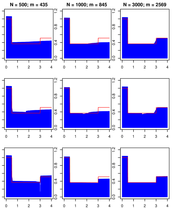
Figure 2:  The true bathtub-shaped hazard rate $\lambda_{1}(t)$ (solid line) given by (31) and the Bayes estimates produced by the APs sampler based on total number of observations, $N=500$ (left column), $1,000$ (middle column) and $3,000$ (right column), with $\theta=0.5,1.75\mbox{ and }3$ (from top row to bottom row).

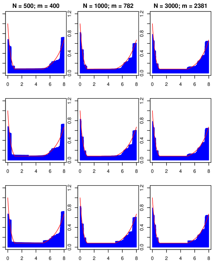
Figure 3:  The true bathtub-shaped hazard rate $\lambda_{2}(t)$ (solid line) given by (32) and the Bayes estimates produced by the APs sampler based on total number of observations, $N=500$ (left column), $1,000$ (middle column) and $3,000$ (right column), with $\theta=1,3\mbox{ and }5$ (from top row to bottom row).

Figure 4:  The true bathtub-shaped hazard rate $\lambda_{1}(t)$ (solid line) given by (31) and the Bayes estimates produced by the SIS methods based on total number of observations, $N=500$ (left column), $1000$ (middle column) and $3000$ (right column), wherein estimates in the first three rows from top to bottom are obtained by the SIPs sampler (Algorithm 3.3) with $\theta=0.5,1.75\mbox{ and }3$, respectively, and those in the last row are obtained by the SIPs$(\theta)$ sampler with an unknown $\theta$.

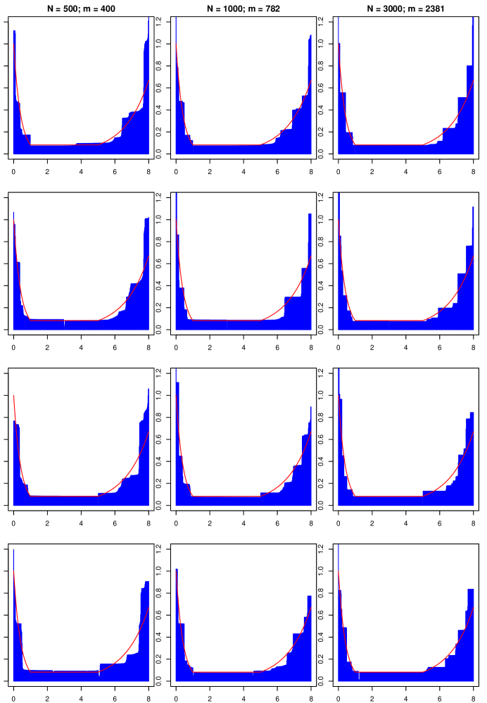
Figure 5:  The true bathtub-shaped hazard rate $\lambda_{2}(t)$ (solid line) given by (32) and the Bayes estimates produced by the SIS methods based on total number of observations, $N=500$ (left column), $1000$ (middle column) and $3000$ (right column), wherein estimates in the first three rows from top to bottom are obtained by the SIPs sampler (Algorithm 3.3) with $\theta=1,3\mbox{ and }5$, respectively, and those in the last row are obtained by the SIPs$(\theta)$ sampler with an unknown $\theta$.

5 A Test of an MFR Versus an BFR

Early references devoted to testing for a constant hazard rate versus an MFR include Proschan and Pyke (1967), Bickel and Doksum (1969) and Gail and Gastwirth (1978a,b), among others. Without relying on exponentiality assumption, Gijbels and Heckman (2004) develop a testing procedure via normalized spacings for testing an MFR against alternatives of some local departures. For testing an MFR versus other general alternatives, Hall and Van Keilegom (2005) propose a calibration method related to the “increasing bandwidth” approach suggested by Silverman (1981) in the case of density estimation. Testing procedures involving BFRs can be found in, for example, Aarset (1985), who discussed the test statistic proposed by Bergman (1979) for testing a constant hazard rate against an BFR, and Vaurio (1999), who proposed a few test statistics for testing between an MFR and other non-monotone alternatives including BFRs.

A Bayesian test of monotone versus bathtub-shaped hazard rates can be readily defined in terms of $\theta$ based on the models in (1) with $\mu$ being a nuisance parameter as follows: Suppose we are interested in testing whether a set of observations ${\bf T}$, defined similarly in Section 2, is generated according to a non-decreasing hazard rate or an BFR. Based on (1), it is equivalent to choose between two hypotheses $H_{0}:\theta=0$ and $H_{1}:\theta\in(0,\infty)$ as when $\theta=0$, models in (1) correspond to a class of non-decreasing hazard rates; otherwise, they give a class of BFRs with a change point $\theta>0$. In particular, the likelihood of the data given $(\mu,\theta)$ under $H_{1}$ is given by (4) when $\theta\neq 0$ or $\infty$, while the likelihood of the data given $\mu$ under $H_{0}$ follows from (4) with $\theta=0$ as

$$e^{-\mu(g_{\smash{\lower 0.5382pt\hbox{{\tiny$N$,{\tiny$0$}}}}})}\prod_{i=1}^{m}\int\mathbb{I}(0<u_{i}\leq T_{i})\mu(du_{i}).$$ (33)

Let $\pi_{0}$ denote the prior probability of $H_{0}$, and then $1-\pi_{0}$ denotes the prior probability of $H_{1}$; furthermore, suppose the mass on $H_{1}$ is spread out according to a distribution $\pi(d\theta)$. Suppose we assume that $\mu$’s under $H_{0}$ and $H_{1}$ are two independent, but not necessarily identical, completely random measures characterized by (2).

Corollary 5.1.

Suppose $\mu$ is a completely random measure characterized by (2). It follows from Theorem 2.3 that the likelihood of the data ${\bf T}$ given $\theta$ is proportional to

$$m_{\theta}({\bf T})={\cal L}_{\mu}(g_{N,\theta}|\rho,\eta)\times\sum_{{\bf S}^{-}}\phi^{-}_{\theta}({{\bf S}^{-}},{\bf T})\times\sum_{{\bf S}^{+}}\phi^{+}_{\theta}({{\bf S}^{+}},{\bf T}).$$ (34)

Hence, the marginal density of ${\bf T}$ is given by

$$m({\bf T})=\pi_{0}\times{\cal L}_{\mu}(g_{N,0}|\rho,\eta)\sum_{{\bf S}^{+}}\phi^{+}_{0}({{\bf S}^{+}},{\bf T})+(1-\pi_{0})\times\int_{\cal{H}}m_{\theta}({\bf T})\pi(d\theta).$$ (35)

It implies that the posterior probability of $H_{0}$ is given by

$$P(H_{0}|{\bf T})=\frac{\pi_{0}\times{\cal L}_{\mu}(g_{N,0}|\rho,\eta)\sum_{{\bf S}^{+}}\phi^{+}_{0}({{\bf S}^{+}},{\bf T})}{m({\bf T})},$$

and that of $H_{1}$ is equal to $1-P(H_{0}|{\bf T})$. Also of interest is the posterior odds of $H_{0}$ to $H_{1}$, which is given by

$$\frac{\pi_{0}}{1-\pi_{0}}\times\frac{{\cal L}_{\mu}(g_{N,0}|\rho,\eta)\sum_{{\bf S}^{+}}\phi^{+}_{0}({{\bf S}^{+}},{\bf T})}{\int_{\cal{H}}m_{\theta}({\bf T})\pi(d\theta)},$$

wherein $\pi_{0}/(1-\pi_{0})$ is the prior odds and the latter ratio is the Bayes factor for $H_{0}$ versus $H_{1}$ (see Kass and Raftery (1995) for a review of Bayes factors).

Regarding implementation of the above Bayesian test, Algorithm 3.2 and the SIP$(\theta)$ sampler can be applied to approximate the marginal density of ${\bf T}$, $m({\bf T})$, in (35), and also the posterior probabilities of $H_{0}$ and $H_{1}$. On one hand, the sum $\sum_{{\bf S}^{+}}\phi_{0}^{+}({\bf S}^{+},{\bf T})$ is approximated by

$$\frac{1}{M}\sum_{i=1}^{M}\sigma_{m-1}({\bf S}_{(i)}),$$

if ${{\bf S}}_{(0)},{{\bf S}}_{(1)},\ldots,{{\bf S}}_{(M)}$ are independent samples obtained via implementing Algorithm 3.2 with $\phi({\bf S})=\phi_{0}^{+}({\bf S},{\bf T})$ in (25) and $\sigma_{m-1}({\bf S}_{(i)})$ defined in (27). On the other hand, the integral $\int_{\cal{H}}m_{\theta}({\bf T})\pi(d\theta)$ is approximated by

$$\frac{1}{M}\sum_{i=1}^{M}\sigma_{m-n_{(i)}-1}({\bf S}^{-}_{(i)}|\theta_{(i)})\,\sigma_{n_{(i)}-1}({\bf S}^{+}_{(i)}|\theta_{(i)})\,\rho(\theta_{(i)}),$$

if $({\bf S}_{(1)}^{-},{\bf S}_{(1)}^{+},\theta_{(1)}),\ldots,({\bf S}_{(M)}^{-},{\bf S}_{(M)}^{+},\theta_{(M)})$ are independent samples obtained via implementing the SIP$(\theta)$ sampler, whereby $n_{(i)}$ is determined in step (S1) after $\theta_{(i)}$ is fixed in step (S0), and $\sigma_{m-n_{(i)}-1}({\bf S}^{-}_{(i)}|\theta_{(i)})$ and $\sigma_{n_{(i)}-1}({\bf S}^{+}_{(i)}|\theta_{(i)})$ are obtained from steps (S2) and (S3), respectively.

6 Proportional Hazards

The Cox regression model [Cox (1972)] is an important example of the multiplicative intensity model that can allow incorporation of covariates, together with right independent censoring, in survival analysis. For Bayes inference of general hazard rates with presence of covariates, see Kalbfleisch (1978), Ibrahim, Chen and MacEachern (1999), James (2003) and Ishwaran and James (2004), among others. Suppose we collect failure data until time $\tau$, which are governed by an underlying hazard rate on $\cal{H}$ associated with a $p$-dimensional covariate vector ${\bf X}\in{\cal{R}}^{p}$,

$$\lambda(t|{\bf X},\mbox{\boldmath{$\beta$}},\mu,\theta)=\lambda(t|\mu,\theta)\exp({\mbox{\boldmath{$\beta$}}}^{T}{\bf X}),$$

where $\lambda(t|\mu,\theta)$ defined in (1) is an unknown baseline hazard rate of a bathtub shape and $\mbox{\boldmath{$\beta$}}\in{\cal{R}}^{p}$ is an unknown parameter vector. The data $\mathbf{D}=((T_{1},{\bf X}_{1}),\ldots,(T_{N},{\bf X}_{N}))$ summarize completely observed failure times $T_{1}<\cdots<T_{m}$ and right-censored times $T_{i}=\tau$, $i=m+1,\ldots,N$, associated with covariate vector ${\bf X}_{i}$, $i=1,\ldots,N$, respectively. Define $f_{\smash{\lower 1.50694pt\hbox{{\scriptsize$N$,\mbox{\boldmath{\scriptsize$\beta$}},\scriptsize$\theta$}}}}(x,u)=g_{\smash{\lower 1.50694pt\hbox{{\scriptsize$N$,\mbox{\boldmath{\scriptsize$\beta$}},\scriptsize$\theta$}}}}(u)x$, for any $(x,u)\in(\cal{H},\cal{R})$, where

$$g_{\smash{\lower 1.50694pt\hbox{{\scriptsize$N$,\mbox{\boldmath{\scriptsize$\beta$}},\scriptsize$\theta$}}}}(u)=\int_{0}^{\tau}\left[\sum_{i=1}^{N}\mathbb{I}(T_{i}\geq t)\exp({\mbox{\boldmath{$\beta$}}}^{T}{\bf X}_{i})\right][\mathbb{I}(t-\theta\leq u<0)+\mathbb{I}(0<u\leq t-\theta)]dt.$$ (36)

Then, the Cox proportional hazards likelihood may be written as

$$\left[\prod_{i=1}^{m}\exp({\mbox{\boldmath{$\beta$}}}^{T}{\bf X}_{i})\lambda(T_{i}|\mu,\theta)\right]\exp\left[-\mu(g_{\smash{\lower 1.50694pt\hbox{{\scriptsize$N$,\mbox{\boldmath{\scriptsize$\beta$}},\scriptsize$\theta$}}}})\right],$$ (37)

where $\mu(g_{\smash{\lower 1.50694pt\hbox{{\scriptsize$N$,\mbox{\boldmath{\scriptsize$\beta$}},\scriptsize$\theta$}}}})=\int_{\cal{R}}g_{\smash{\lower 1.50694pt\hbox{{\scriptsize$N$,\mbox{\boldmath{\scriptsize$\beta$}},\scriptsize$\theta$}}}}(u)\mu(du)=\int_{0}^{\tau}[\sum_{i=1}^{N}\mathbb{I}(T_{i}\geq t)\exp({\mbox{\boldmath{$\beta$}}}^{T}{\bf X}_{i})]\lambda(t|\mu,\theta)dt$. Assume$\int_{\cal{R}}x^{\ell}e^{-g_{\smash{\lower 0.5382pt\hbox{{\tiny$N$,\mbox{\boldmath{\tiny$\beta$}},\tiny$\theta$}}}}(u)x}\rho(dx|u)<\infty$, for $\ell=1,\ldots,m$ and a fixed $u>0$. If $\pi(d\mbox{\boldmath{$\beta$}})$ and $\pi(d\theta)$ are independent priors for $\beta$ and $\theta$, applying the same arguments in proving Theorems 2.1 and 2.3 yields that the law of $\mu|\mathbf{D}$ is equivalent to that of a random measure $\mu_{g_{\smash{\lower 0.5382pt\hbox{{\tiny$N$,\mbox{\boldmath{\tiny$\beta$}},\tiny$\theta$}}}}}+\sum_{\{j^{\ast}|{\bf S}^{-}\}}Q_{j}^{-}\delta_{y_{j}^{-}}+\sum_{\{j^{\ast}|{\bf S}^{+}\}}Q_{j}^{+}\delta_{y_{j}^{+}}$, where $\mu_{g_{\smash{\lower 0.5382pt\hbox{{\tiny$N$,\mbox{\boldmath{\tiny$\beta$}},\tiny$\theta$}}}}}$, with law denoted by $\mathbb{P}(d\mu_{g_{\smash{\lower 0.5382pt\hbox{{\tiny$N$,\mbox{\boldmath{\tiny$\beta$}},\tiny$\theta$}}}}})$, is a completely random measure with Lévy measure $e^{-g_{\smash{\lower 0.5382pt\hbox{{\tiny$N$,\mbox{\boldmath{\tiny$\beta$}},\tiny$\theta$}}}}(u)x}\rho(dx|u)\eta(du)$. It is determined by the law of$\mu_{g_{\smash{\lower 0.5382pt\hbox{{\tiny$N$,\mbox{\boldmath{\tiny$\beta$}},\tiny$\theta$}}}}},{\bf Q}^{-},{\bf y}^{-},{\bf S}^{-},{\bf Q}^{+},{\bf y}^{+},{\bf S}^{+},\theta,\mbox{\boldmath{$\beta$}}|\mathbf{D}$, which is proportional to

$$\mathbb{P}(d\mu_{g_{\smash{\lower 0.5382pt\hbox{{\tiny$N$,\mbox{\boldmath{\tiny$\beta$}},\tiny$\theta$}}}}})\pi(d\theta)\pi(d\mbox{\boldmath{$\beta$}}){\cal L}_{\mu}(g_{\smash{\lower 1.50694pt\hbox{{\scriptsize$N$,\mbox{\boldmath{\scriptsize$\beta$}},\scriptsize$\theta$}}}}|\rho,\eta)\prod_{i=1}^{m}\exp({\mbox{\boldmath{$\beta$}}}^{T}{\bf X}_{i})$$

$$\times|{\mathbb{C}}_{{\bf S}^{-}}|\prod_{\{j^{\ast}|{\bf S}^{-}\}}\left\{({Q_{j}^{-}})^{m_{j}^{-}}e^{-g_{\smash{\lower 0.5382pt\hbox{{\tiny$N$,{\tiny$\theta$}}}}}(y_{j}^{-})Q_{j}^{-}}\rho(dQ_{j}^{-}|y_{j}^{-})\mathbb{I}(Z_{j}^{\theta}\leq y_{j}^{-}<0)\eta(dy_{j}^{-})\right\}$$

$$\times|{\mathbb{C}}_{{\bf S}^{+}}|\prod_{\{j^{\ast}|{\bf S}^{+}\}}\left\{({Q_{j}^{+}})^{m_{j}^{+}}e^{-g_{\smash{\lower 0.5382pt\hbox{{\tiny$N$,{\tiny$\theta$}}}}}(y_{j}^{+})Q_{j}^{+}}\rho(dQ_{j}^{+}|y_{j}^{+})\mathbb{I}(0<y_{j}^{+}\leq Y_{j}^{\theta})\eta(dy_{j}^{+})\right\}.$$

Analogous results with presence of covariates of Theorems 2.1 and 2.3 in terms of two ${\bf S}$-paths can be obtained via Bayes’ theorem and multiplication rule.

Proposition 6.1.

Suppose the likelihood of the data is given by (37). Assume that $\mu$ is a completely random measure characterized by the Laplace functional (2), and independently, let $\pi(d\mbox{\boldmath{$\beta$}})$ and $\pi(d\theta)$ denote independent priors for $\beta$ and $\theta$. Then,

1. the law of $\mu|\theta,\mbox{\boldmath{$\beta$}},\mathbf{D}$ can be described by a three-step hierarchical experiment as in Theorem 2.1, of which $f_{\smash{\lower 1.50694pt\hbox{{\scriptsize$N$,{\scriptsize$\theta$}}}}}(\cdot,\cdot)$ and $g_{\smash{\lower 1.50694pt\hbox{{\scriptsize$N$,{\scriptsize$\theta$}}}}}(\cdot)$ are replaced by $f_{\smash{\lower 1.50694pt\hbox{{\scriptsize$N$,\mbox{\boldmath{\scriptsize$\beta$}},\scriptsize$\theta$}}}}(\cdot,\cdot)$ and $g_{\smash{\lower 1.50694pt\hbox{{\scriptsize$N$,\mbox{\boldmath{\scriptsize$\beta$}},\scriptsize$\theta$}}}}(\cdot)$, respectively.

2. the law of $\theta|\mbox{\boldmath{$\beta$}},\mathbf{D}$ is characterized by, for any Borel set $B\in\cal{H}$,

   $$\Pr(\theta\in B|\mbox{\boldmath{$\beta$}},\mathbf{D})=\int_{B}\sum_{{\bf S}^{-}}\sum_{{\bf S}^{+}}\pi({\bf S}^{-},{\bf S}^{+},d\theta|\mbox{\boldmath{$\beta$}},\mathbf{D}),$$

   where $\pi({\bf S}^{-},{\bf S}^{+},d\theta|\mbox{\boldmath{$\beta$}},\mathbf{D})\propto{\cal L}_{\mu}(g_{\smash{\lower 1.50694pt\hbox{{\scriptsize$N$,\mbox{\boldmath{\scriptsize$\beta$}},\scriptsize$\theta$}}}}|\rho,\eta)\times|\mathbb{C}_{{\bf S}^{-}}|\prod_{\{j^{\ast}|{\bf S}^{-}\}}\int_{Z^{\theta}_{j}}^{0}\kappa_{m_{j}^{-}}(e^{-f_{\smash{\lower 0.5382pt\hbox{{\tiny$N$,\mbox{\boldmath{\tiny$\beta$}},\tiny$\theta$}}}}}\rho|y)\eta(dy)\break\times|\mathbb{C}_{{\bf S}^{+}}|\prod_{\{j^{\ast}|{\bf S}^{+}\}}\int_{0}^{Y^{\theta}_{j}}\kappa_{m_{j}^{+}}(e^{-f_{\smash{\lower 0.5382pt\hbox{{\tiny$N$,\mbox{\boldmath{\tiny$\beta$}},\tiny$\theta$}}}}}\rho|y)\eta(dy)\times\pi(d\theta)$.

To evaluate any posterior quantities of model (37), such as the posterior mean of the underlying bathtub-shaped baseline hazard rate and the posterior mean of the covariate parameters $\beta$, run the following Gibbs sampler to obtain random samples from the posterior distribution of $({\bf Q}^{-},{\bf y}^{-},{\bf S}^{-},{\bf Q}^{+},{\bf y}^{+},{\bf S}^{+},\theta,\mbox{\boldmath{$\beta$}})$ given $\mathbf{D}$:

1. Draw ${\bf S}^{-},{\bf S}^{+}|{\bf Q}^{-},{\bf y}^{-},{\bf Q}^{+},{\bf y}^{+},{\bf S}^{+},\theta,\mbox{\boldmath{$\beta$}},\mathbf{D}$ by independently implementing Algorithm 3.1 as in steps (M1) and (M2) in Section 3.1.1.

2. Draw ${\bf Q}^{-},{\bf y}^{-},{\bf Q}^{+},{\bf y}^{+}|{\bf S}^{-},{\bf S}^{+},\theta,\mbox{\boldmath{$\beta$}},\mathbf{D}$ according to the analogues of the conditional distributions (12–15) in Theorem 2.1 with $f_{\smash{\lower 1.50694pt\hbox{{\scriptsize$N$,{\scriptsize$\theta$}}}}}(\cdot,\cdot)$ and $g_{\smash{\lower 1.50694pt\hbox{{\scriptsize$N$,{\scriptsize$\theta$}}}}}(\cdot)$ replaced by $f_{\smash{\lower 1.50694pt\hbox{{\scriptsize$N$,\mbox{\boldmath{\scriptsize$\beta$}},\scriptsize$\theta$}}}}(\cdot,\cdot)$ and $g_{\smash{\lower 1.50694pt\hbox{{\scriptsize$N$,\mbox{\boldmath{\scriptsize$\beta$}},\scriptsize$\theta$}}}}(\cdot)$, respectively.

3. Draw $\theta|{\bf Q}^{-},{\bf y}^{-},{\bf S}^{-},{\bf Q}^{+},{\bf y}^{+},{\bf S}^{+},\mbox{\boldmath{$\beta$}},\mathbf{D}$ from the density proportional to

   $$\pi(d\theta){\cal L}_{\mu}(g_{\smash{\lower 1.50694pt\hbox{{\scriptsize$N$,\mbox{\boldmath{\scriptsize$\beta$}},\scriptsize$\theta$}}}}|\rho,\eta)\prod_{\{j^{\ast}|{\bf S}^{-}\}}e^{-g_{\smash{\lower 0.5382pt\hbox{{\tiny$N$,\mbox{\boldmath{\tiny$\beta$}},\tiny$\theta$}}}}(y_{j}^{-})Q_{j}^{-}}\mathbb{I}(Z^{\theta}_{j}-\theta\leq y_{j}^{-})\prod_{\{j^{\ast}|{\bf S}^{+}\}}e^{-g_{\smash{\lower 0.5382pt\hbox{{\tiny$N$,\mbox{\boldmath{\tiny$\beta$}},\tiny$\theta$}}}}(y_{j}^{+})Q_{j}^{+}}\mathbb{I}(y^{+}_{j}\leq Y^{\theta}_{j}-\theta).$$

4. Draw $\mbox{\boldmath{$\beta$}}|{\bf Q}^{-},{\bf y}^{-},{\bf S}^{-},{\bf Q}^{+},{\bf y}^{+},{\bf S}^{+},\theta,\mathbf{D}$ from the density proportional to

   $$\pi(d\mbox{\boldmath{$\beta$}}){\cal L}_{\mu}(g_{\smash{\lower 1.50694pt\hbox{{\scriptsize$N$,\mbox{\boldmath{\scriptsize$\beta$}},\scriptsize$\theta$}}}}|\rho,\eta)\prod_{i=1}^{m}\exp({\mbox{\boldmath{$\beta$}}}^{T}{\bf X}_{i})\prod_{\{j^{\ast}|{\bf S}^{-}\}}e^{-g_{\smash{\lower 0.5382pt\hbox{{\tiny$N$,\mbox{\boldmath{\tiny$\beta$}},\tiny$\theta$}}}}(y_{j}^{-})Q_{j}^{-}}\prod_{\{j^{\ast}|{\bf S}^{+}\}}e^{-g_{\smash{\lower 0.5382pt\hbox{{\tiny$N$,\mbox{\boldmath{\tiny$\beta$}},\tiny$\theta$}}}}(y_{j}^{+})Q_{j}^{+}}.$$

Note that $g_{\smash{\lower 1.50694pt\hbox{{\scriptsize$N$,\mbox{\boldmath{\scriptsize$\beta$}},\scriptsize$\theta$}}}}(u)$ is again a piecewise linear function of $u$ as $g_{\smash{\lower 1.50694pt\hbox{{\scriptsize$N$,{\scriptsize$\theta$}}}}}(u)$ in the case without covariates. This does not create any complexities in evaluating integrals at steps 1 and 2 of the above Gibbs sampler (see discussion of Remark 5.1 in Ho (2006a)). Step 4 above, which is of the same form as the step 4 (for conditional draws of regression parameters $\beta$) of the Blocked Gibbs algorithm suggested by Ishwaran and James (2004, page 184), can be dealt with via a Metropolis step, while step 3 can also be done similarly as the density looks like the one in step 4.

References

• [1] Aalen, O. (1975), “Statistical Inference for a Family of Counting Processes,” Unpublished Ph.D. thesis, University of California, Berkeley.
• [2] Aalen, O. (1978), “Nonparametric Inference for a Family of Counting Processes,” The Annals of Statistics, 6, 701-726.
• [3] Aarset, M. V. (1985), “The Null Distribution of a Test of Constant Versus Bathtub-Failure Rate,” The Scandinavian Journal of Statistics, 12, 55-62.
• [4] Amman, L. (1984), “Bayesian Nonparametric Inference for Quantal Response Data,” The Annals of Statistics, 12, 636-645.
• [5] Barlow, R. E., Bartholomew, D. J., Bremner, J. M., and Brunk, H. D. (1972), Statistical Inference Under Order Restrictions, New York: John Wiley & Sons.
• [6] Barron, A., Schervish, M. J., and Wasserman, L. (1999), “The Consistency of Posterior Distributions in Nonparametric Problems,” The Annals of Statistics, 27, 536-561.
• [7] Bergman, B. (1979), “On Age replacement and the Total Time on Test Concept,” The Scandinavian Journal of Statistics, 6, 161-168.
• [8] Bickel, P. J., and Doksum, K. A. (1969), “Tests for Monotone Failure Rate Based on Normalized Spacings,” The Annals of Mathematics and Statistics, 40, 1216-1235.
• [9] Brunner, L. J. (1992), “Bayesian Nonparametric Methods for Data From a Unimodal Density,” Statistics & Probability Letters, 14, 195-199.
• [10] Brunner, L. J., and Lo, A. Y. (1989), “Bayes Methods for a Symmetric Unimodal Density and its Mode,” The Annals of Statistics, 17, 1550-1566.
• [11] Cox, D. R. (1972), “Regression Models and Life-tables (With Discussion),” Journal of the Royal Statistical Society, Ser. B, 34, 187-220.
• [12] Doksum, K. A. (1974), “Tailfree and Neutral Random Probabilities and Their Posterior Distributions,” The Annals of Probability, 2, 183-201.
• [13] Drǎgichi, L., and Ramamoorthi, R. V. (2003), “Consistency of Dykstra-Laud Priors,” Sankhyā, Ser. A, 65, 464-481.
• [14] Dykstra, R. L., and Laud, P. (1981), “A Bayesian Nonparametric Approach to Reliability,” The Annals of Statistics, 9, 356-367.
• [15] Ferguson, T. S., and Phadia, E. G. (1979), “Bayesian Nonparametric Estimation Based on Censored Data,” The Annals of Statistics, 7, 163-186.
• [16] Gail, M. H., and Gastwirth, J. L. (1978a), “A Scale-free Goodness-of-fit Test for the Exponential Distribution Based on the Gini Statistic,” Journal of the Royal Statistical Society, Ser. B, 40, 350-357.
• [17] —— (1978b), “A Scale-free Goodness-of-fit Test for the Exponential Distribution Based on the Lorenz Curve,” Journal of the American Statistical Association, 73, 787-793.
• [18] Ghosh, J. K., and Ramamoorthi, R. V. (2003), Bayesian Nonparametrics, New York: Springer.
• [19] Gijbels, I., and Heckman, N. (2004), “Nonparametric Testing for a Monotone Hazard Function via Normalized Spacings,” Journal of Nonparametric Statistics, 16, 463-478.
• [20] Hall, P., and Van Keilegom, I. (2005), “Testing for Monotone Increasing Hazard Rate,” The Annals of Statistics, 33, 1109-1137.
• [21] Haupt, E., and Schabe, H. (1997), “The TTT Transformation and a new Bathtub Distribution Model,” Journal of Statistical Planning and Inference, 60, 229-240.
• [22] Hjort, N. L. (1990), “Nonparametric Bayes Estimators Based on Beta Processes in Models for Life History Data,” The Annals of Statistics, 18, 1259-1294.
• [23] Ho, M.-W. (2002), “Bayesian Inference for Models With Monotone Densities and Hazard Rates,” unpubished Ph.D. thesis, The Hong Kong University of Science and Technology, Dept. of Information and Systems Management.
• [24] —— (2006a), “A Bayes Method for a Monotone Hazard Rate via ${\bf S}$-paths,” The Annals of Statistics, 34, 820-836.
• [25] —— (2006b), “Bayes Estimation of a Symmetric Unimodal Density via ${\bf S}$-paths,” Journal of Computational and Graphical Statistics, 15, 848-860.
• [26] —— (2006c), “Bayesian Nonparametric Estimation of a Unimodal Density via two ${\bf S}$-paths,” submitted.
• [27] Ibrahim, J. G., Chen, M.-H., and MacEachern, S. N. (1999), “Bayesian Variable Selection for Proportional Hazards Models,” Canadian Journal of Statistics, 37, 701-717.
• [28] Ishwaran, H., and James, L. F. (2003), “Generalized Weighted Chinese Restaurant Processes for Species Sampling Mixture Models,” Statistica Sinica, 13, 1211-1235.
• [29] —— (2004), “Computational Methods for Multiplicative Intensity Models Using Weighted Gamma Processes: Proportional Hazards, Marked Point Processes, and Panel Count Data,” Journal of the American Statistical Association, 99, 175-190.
• [30] James, L. F. (2003), “Bayesian Calculus for Gamma Processes With Applications to Semiparametric Intensity Models,” Sankhyā, Ser. A, 65, 196-223.
• [31] —— (2005), “Bayesian Poisson Process Partition Calculus With an Application to Bayesian Lévy Moving Averages,” The Annals of Statistics, 33, 1771-1799.
• [32] Kalbfleisch, J. D. (1978), ”Non-parametric Bayesian Analysis of Survival Time Data,” Journal of the Royal Statistical Society, Ser. B, 40, 214-221.
• [33] Kalbfleisch, J. D., and Prentice, R. L. (1980), The Statistical Analysis of Failure Time Data, New York: John Wiley and Sons.
• [34] Kaplan, E. L., and Meier, P. (1958), “Nonparametric Estimation from Incomplete Observations,” Journal of the American Statistical Association, 53, 457-481.
• [35] Kass, R. E., and Raftery, A. E. (1995), “Bayes Factors and Model Uncertainty,” Journal of the American Statistical Association, 90, 773-795.
• [36] Kingman, J. F. C. (1967), Completely random measures. Pacific Journal of Mathematics, 21, 59–78.
• [37] Kingman, J. F. C. (1993), Poisson Processes, Oxford: Oxford University Press.
• [38] Kong, A., Liu, J. S., and Wong, W. H. (1994), “Sequential Imputations and Bayesian Missing Data Problems,” Journal of the American Statistical Association, 89, 278-288.
• [39] Lai, C. D., Xie, M., and Murthy, D. N. P. (2001), “Bathtub-shaped Failure Rate Distributions,” in Handbook of Statistics (Edited by N. Balakrishnan and C. R. Rao). (vol. 20), pp. 69-104, London: Elsevier.
• [40] Laud, P., Damien, P., and Walker, S. G. (2006), “Computations via Auxiliary Random Functions for Survival Models,” The Scandinavian Journal of Statistics, 33, 219-226.
• [41] Lawless, J. F. (1982), Statistical Methods and Methods for Life Time Data, New York: Wiley.
• [42] Liu, J., and Chen, R. (1998), “Sequential Monte Carlo Methods for Dynamic Systems,” Journal of the American Statistical Association, 93, 1032-1044.
• [43] Lo, A. Y., and Weng, C. S. (1989), “On a Class of Bayesian Nonparametric Estimates: II. Hazard Rate Estimates,” Annals of the Institute of Statistical Mathematics, 41, 227-245.
• [44] Meyn, S. P., and Tweedie, R. L. (1993), Markov Chains and Stochastic Stability, Berlin: Springer.
• [45] Mitra, M., and Basu, S. K. (1995), “Change Point Estimation in Non-monotonic Aging Models,” Annals of the Institute of Statistical Mathematics, 47, 483-491.
• [46] Nelson, W. B. (1969), “Hazard Plotting for Incomplete Failure Data,” Journal of Quality Technology, 1, 27-52.
• [47] Proschan, F., and Pyke, R. (1967), “Tests for Monotone Failure Rate,” Fifth Berkeley Symposium, 3, 293-313.
• [48] Rajarshi, S., and Rajarshi, M. B. (1988), “Bathtub Distributions: a Review,” Communications in Statistics. Theory and Methods, 17, 2597-2621.
• [49] Reboul, L. (2005), “Estimation of a Function Under Shape Restrictions. Applications to Reliability,” The Annals of Statistics, 33, 1330-1356.
• [50] Silverman, B. W. (1981), “Using Kernel Density Estimates to Investigate Multimodality,” Journal of the Royal Statistical Society, Ser. B, 43, 97-99.
• [51] Singpurwalla, N. D. (2006), Reliability and Risk: a Bayesian Perspective, John Wiley and Sons.
• [52] Sinha, D., and Dey, D. K. (1997), “Semiparametric Bayesian Analysis of Survival Data,” Journal of the American Statistical Association, 92, 1195-1212.
• [53] Susarla, V., and Van Ryzin, J. (1976), “Nonparametric Bayesian Estimation of Survival Curves from Inomplete Observations,” Journal of the American Statistical Association, 71, 897-902.
• [54] Tanner, M. A., and Wong, W. H. (1983), “The Estimation of the Hazard Function From Randomly Censored Data by the Kernel Method,” The Annals of Statistics, 11, 989-993.
• [55] Vaurio, J. K. (1999), “Indentification of Process and Distribution Characteristics by Testing Monotonic and Non-monotonic Trends in Failure Intensities and Hazard Rates,” Reliability Engineering & System Safety, 64, 345-357.
• [56] Watson, G. S., and Leadbetter, M. R. (1964a), “Hazard Analysis I,” Biometrika, 51, 175-184.
• [57] —— (1964b), “Hazard Analysis II,” Sankhyā, Ser. A, 26, 101-116.
• [58] Wolpert, R. L., and Ickstadt, K. (1998), “Poisson/Gamma Random Field Models for Spatial Statistics,” Biometrika, 85, 251-267.
• [59] Yandell, B. S. (1983), “Nonparametric Inference for Rates With Censored Survival Data,” The Annals of Statistics, 11, 1119-1135.